qGaussian: Tools to Explore Applications of Tsallis Statistics

Abstract

$q$-Gaussian distribution appear in many science areas where we can find systems that could be described within a nonextensive framework. Usually, a way to assert that these systems belongs to nonextensive framework is by means of numerical data analysis. To this end, we implement random number generator for $q$-Gaussian distribution, while we present how to computing its probability density function, cumulative density function and quantile function besides a tail weight measurement using robust statistics.

1 Introduction

Entropy is a fundamental concept in physics since it is in essence of second law of thermodynamics. In the article ’Possible generalization of Boltzmann-Gibbs statistics’ [1], was postulated the Tsallis entropy $S_{q}[p(x)]=(q-1)^{-1}*(1-\int_{-\infty}^{\infty}p^{q}(x)dx)$. Within the nonextensive approach, the sum of the entropy of two independent subsystems is given by: $S_{q}(a+b)=S_{q}(a)+S_{q}(b)+(1-q)S_{q}(a)S_{q}(b)$, where $q$ is an entropic index. The $q$-Gaussian density function $p(x)$, presented in the next section, arises from maximizing the $q$-entropy functional $S_{q}[p(x)]$ under constraints [2] and [3] and it is important at the framework of the nonextensive statistical mechanics.

There is a broad literature where the nonextensive approach is used to model systems and/or explain many-body problems and issues related to chaos. In some cases, there exist strong evidences that theory works, certified by a broad numerical decade from experimental measurements or numericals simulation that let us obtain a $q$ value by an almost flawless curve fitting. In other cases, a lot of observational data are only suggestive of a nonextensive approach. A myriad of examples can be found in [4] and [2]. This work aims to spread among users of R, a statistical package that deals with the distribution of $q$-Gaussian, allowing researchers to infer and evaluate, from empirical data, a nonextensive behaviour.

At section theoretical background, we first see a way to represent the probability density function and how to write the cumulative density function and quantile function using the Beta function. Then, we present the random number generator and a way to identify the $q$-Gaussian at empirical data. Next, we will see the implementation in R of all subjects described previously. Lastly, illustrative examples section present the density function shape, after the comparison among $q$-Gaussian with its special cases and an estimate of $q$ value is made up from a data set.

2 Theoretical background

The $q$-Gaussian probability density function, named here $q$PDF [5], with $q$-mean $\mu_{q}$ and $q$-variance $\sigma_{q}$ can be written as:

$$p(x;\mu_{q},\sigma_{q})=\frac{1}{\sigma_{q}{\text{B}}\left(\frac{\alpha}{2},\frac{1}{2}\right)}\sqrt{\frac{|Z|}{u^{(1+1/Z)}}}$$ (1)

where $Z=(q-1)/(3-q)$,

$$\alpha=\left\{\begin{array}[]{ll}1-1/Z&\textrm{if $q<1$},\\ 1/Z&\textrm{if $1<q<3$},\\ \end{array}\right.$$

$u(x)=1+Z(x-\mu_{q})^{2}/\sigma^{2}_{q}$, and $\text{B}(a,b)$ is the Beta function . In the limit of $q\rightarrow 1$ a $q$PDF tends to a standard Gaussian distribution. For $q<1$, it is a compact support distribution, with $x\in[\pm\sigma_{q}/\sqrt{-Z}]$. When $1<q<3$, it is a heavy tail. In the last case, a power law asymptotic behaviour describes well this class of distribution.

Given $X=(x_{1},x_{2},...x_{n})$ a random variable, the cumulative distribution function ($q$CDF), $F(x)=P[X<x]$

$$F(x)=\int_{-\infty}^{x}p(v)dv,$$

could be represented through $\text{I}_{w}(a,b)$, the regularized incomplete Beta function [6]:

$$F(x;\mu_{q};\sigma_{q})=\left\{\begin{array}[]{ll}\frac{1}{2}\text{I}_{\beta}\left(\frac{\alpha}{2},\frac{1}{2}\right)&\textrm{if $x<\mu_{q}$},\\ 1-\frac{1}{2}\text{I}_{\beta}\left(\frac{\alpha}{2},\frac{1}{2}\right)&\textrm{if $x>\mu_{q}$},\\ \end{array}\right.$$ (2)

where

$$\beta=\left\{\begin{array}[]{ll}u(x)&\textrm{if $q<1$},\\ 1/u(x)&\textrm{if $1<q<3$}.\\ \end{array}\right.$$

In third, the quantile function ($q$QF) is obtained as an inverse function of $y=F(x)$, $w=\text{I}^{-1}_{2y}(\frac{\alpha}{2},\frac{1}{2})$:

$$C(y;\mu_{q},\sigma_{q})=\left\{\begin{array}[]{ll}\mu_{q}-\sigma_{q}^{2}\sqrt{\left(\gamma-1\right)/Z}&\textrm{if $y<1/2$},\\ \mu_{q}+\sigma_{q}^{2}\sqrt{\left(\gamma-1\right)/Z}&\textrm{if $1-y<1/2$},\\ \end{array}\right.$$ (3)

where

$$\gamma=\left\{\begin{array}[]{ll}\text{I}^{-1}_{2y}\left(\frac{\alpha}{2},\frac{1}{2}\right)&\textrm{if $q<1$},\\ 1/\text{I}^{-1}_{2y}\left(\frac{\alpha}{2},\frac{1}{2}\right)&\textrm{if $1<q<3$}.\\ \end{array}\right.$$

It is worth calling attention despite the fact that $q$CDF and $q$QF obtained from a compact support distribution do not appear explicitly shown in [3], these could be deduced by the same straightforward method presented in it.

The random numbers generator from a $q$PDF can be implemented in different ways. The straightforward method use the quantile function to creates random sample elements $x_{i}=C(y_{i};\mu_{q},\sigma_{q})$, where $y_{i}\in[0,1]$ are obtained from a uniform random number. In the second way, we use the Box-Muller algorithm as presented in [7] with the Mersenne-Twister algorithm as a uniform random number generator to create a $q$-Gaussian random variable $X\equiv N_{q}(\mu_{q},\sigma_{q})\equiv\mu_{q}+\sigma_{q}N_{q}(0,1)$ where $N_{q}(0,1)$ is called standard $q$-Gaussian.

The classical kurtosis methods, when applied to a data set, are very sensitive to outlying values, however, it is possible to diminish this problem at a measurement of the tail heaviness by using robust statistic concepts. To doing that, given a sorted sample $\{x_{1}<\dots<\tilde{x}<\dots<x_{n}\}$ from a univariate distribution with median $\tilde{x}$, [8] established the medcouple to evaluates the tail weight when applied to $\{x_{1}<\dots<\tilde{x}\}$ and $\{\tilde{x}<\dots<x_{n}\}$. This procedure can be applied to characterize the $q$-Gaussian with heavy tail and compact support. To this end, [5] aiming to identify a $q$-Gaussian distribution at empirical data, proposed a relationship between medcouple and $q$ value obtained by curve fitting.

3 R implementation

The main goal of the package qGaussian it is lets us to compute $q$PDF (1), $q$CDF (2) and $q$QF (3) as same time generates random numbers from a $q$-Gaussian distribution parametrised by $q$ value. To compute the Beta function and its inverse it is necessary the zipfR package, while the robustbase is the package of robust statistic to implement a tail weight measurement.

Quantity	R’s commands
$p(x)$	dqgauss(x,q,mu,sig)
$F(x)$	pqgauss(x,q,mu,sig,lower.tail=T)
$C(y)$	cqgauss(y,q,mu,sig,lower.tail=T)
$x_{i}$	rqgauss(n,q,mu,sig,meth="Box-Muller")
$q$	qbymc(X)

Table 1: Sintaxe of R’s commands for each output quantities

In table 1, the input argument x represent a vector of quantiles for instructions dqgauss(x,..) and pqgauss(x,..) while y represent a vector of probabilities and n the length sample, for the random number generator. The parameters q, mu and sig are the entropic index, $q$-mean and $q$-variance, respectively, assuming the default values $(0,0,1)$. The medcouple is used into the qbymc(X) code to estimate $q$ value and standard error, receiving a random variable X, from the class "vector", as input. We will see below, all the R’s commands described above.

4 Illustrative and demonstrative examples

First of all, two packages should be loaded.
library(robustbase)
library(zipfR)

After, we start examples section presenting the shape of the $q$PDF plotted for typical $q$ values over a quantile range covering more that $99.9\%$ of area of the standard Gaussian. Besides that, we create a random sample with $q=0$ then we choose the appropriate class intervals to create the histogram that is plotted against the $q$PDF.

$\#\#\#$ Plot six qPDFs
qv <- c(2.8, 2.5, 2, 1.01, 0, -5); nn <- 700
xrg <- sqrt((3-qv[6])/(1-qv[6]))
xr <- seq(-xrg, xrg, by = 2*xrg/nn)
y0 <- dqgauss(xr, qv[6])
plot(xr, y0, ty = ’l’, xlim = range(-4.5, 4.5), ylab = ’p(x)’, xlab = ’x’)
for (i in 1:5)
if (qv[i] < 1) xrg <- sqrt((3-qv[i])/(1-qv[i]))
else xrg <- 4.5
vby <- 2*xrg/nn
xr <- seq(-xrg, xrg, by = 2*xrg/nn)
y0 <- dqgauss(xr, qv[i])
points (xr, y0, ty = ’l’, col = (i+1))

legend(2, 0.4, legend = c(expression(paste(q == -5)), expression(paste(q == 0)),
expression(paste(q == 1.01)), expression(paste(q == 2)),
expression(paste(q == 2.5)), expression(paste(q == 2.8))),
col = c(1, 6, 5, 4, 3, 2), lty = c(1,1,1,1,1,1)
)

$\#\#\#$ qPDF Histogram for q = 0
qv <- 0
rr <- rqgauss(2$\wedge$16, qv)
nn <- 70
xrg <- sqrt((3-qv)/(1-qv))
vby <- 2*xrg/(nn)
xr <- seq(-xrg, xrg, by = vby)
hist (rr, breaks = xr, freq = FALSE, xlab = "x", main = ”)
y <- dqgauss(xr)
lines(xr, y/sum(y*vby), cex = .5, col = 2, lty = 4)

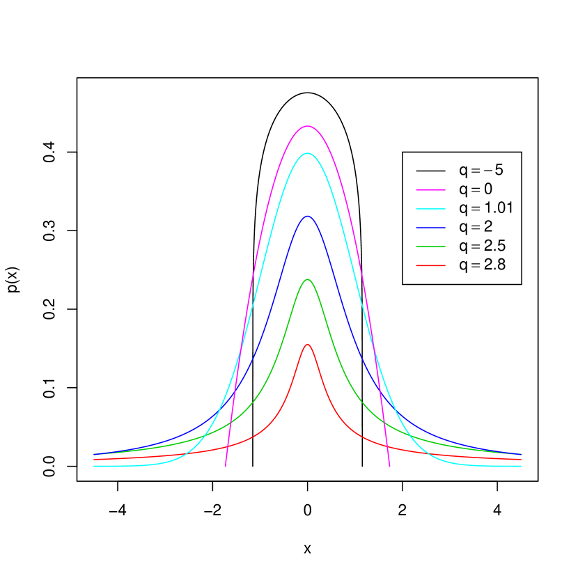
(a) p(x) for typical $q$ values

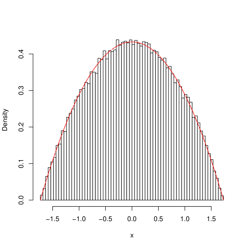
(b) Histogram and $q$PDF for $q=0$

Figure 1: The standard q-Gaussian distribution shapes for representatives values of $q$, and a histogram with rqgauss(n, q = 0)

In the next example, we compare $q$-Gaussian against two particular cases. The $q$-Gaussian is related with Student’s-t distribution by $q=(3+\text{df})/(1+\text{df})$ and Cauchy ($q=2$) [9] and [10]. At theses codes, first we can seen how Student’s-t distribution is a particular case of a more general distribution, using the standard $q$PDF as model. We generate a random sample by means R stats package using the command rt(n,df) with length n for df degree of freedom. At second, the cumulative Cauchy distribution is presented versus rqgauss random number generator.

$\#\#\#$ qGaussian versus Student-t
set.seed(1234)
sam <- 1000; df <- 7
r <- rt(sam, df)
qv <- (df+3)/(df+1)
plot(sort(r), (1:sam/sam), main = "qCDF vs rt", col = "blue",
ylab = "Probability", xlim = range(-4.5, 4.5), xlab = ’x’)
x <- seq(min(r), max(r), length = 313)
lines(x, pqgauss(x, qv), lwd = 2)
legend(1.5, 0.7, legend = c(expression(paste(q == 1.25)), expression(paste(df == 7))),
col = c("black", "blue"), lty = c(1, 0), lwd = 1, pch = c(-1, 1))
$\#\#\#$ qGaussian versus Cauchy
set.seed(1234)
sam <- 1000
r2 <- rcauchy(sam, 100)
x2 <- 1:sam/sam
plot(x2, sort(r2), main = "qQF vs rcauchy", col = "red",
xlab = "Probability", ylim = range(70, 160), ylab = ’x’)
lines(x2, cqgauss(x2, mu = 100, q = 2), lwd = 2)
legend(.3, 145, col = c("black", "red"), lty = c(1, 0), lwd = 1, pch = c(-1, 1),
legend = c(expression(paste(’q == 2’)), expression(paste(’rcauchy(n, 100)’))))

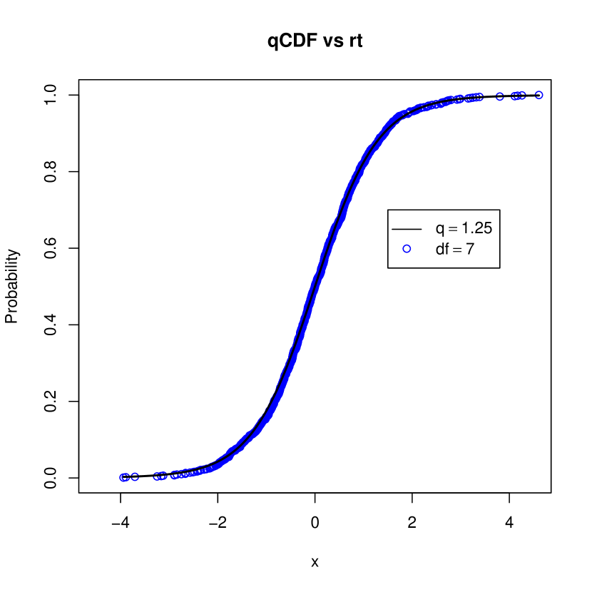
(a) The blue dots was created from Student’s-t random generator,rt(..), and fitted with a $q$CDF

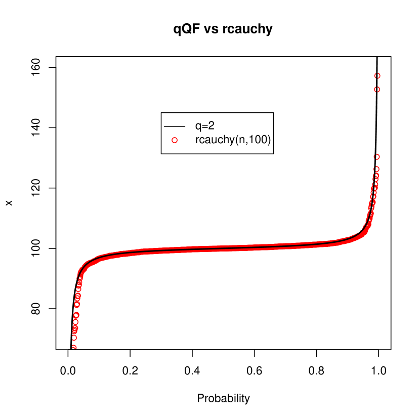
(b) The solid line, $q$QF, matches with the red dots generated using rcauchy command.

Figure 2: Comparison of $q$-Gaussian against two specials cases

In the third example, we will figure out how estimate the $q$ value for a random sample using the qbymc(X) command. For that, we generate a synthetic data with parameters $q=1.39$ and length $n=2004$. After, it is shown that the value of $q$ and its standard error that went obtained remain unchanged, regardless of the values chosen for $q$-mean and $q$-variance.

$\#\#\#$ Identifying a random sample
set.seed(1000)
qbymc(rqgauss(2004, 1.39))
Estimate Std. Error
1.411094 0.109256

$\#\#\#$ Identifying a random sample regardless q and mu
set.seed(1000)
qbymc(rqgauss(2004, 1.39, 3.141592, 2.718281))
Estimate Std. Error
1.411094 0.109256

5 Summary

In this work, we create a statistical package for $q$-Gaussian distribution following the pattern of R stats packages. Also, was included an algorithm that is used to identify $q$PDF at an empirical data set. Moreover, we hope to include in future releases, other mathematical topics related to $q$ algebra and others nonextensive distributions.

References

- [1] C. Tsallis, Possible generalization of boltzmann-gibbs statistics, J. Stat. Phys. 52 (1/2) (1988) 479.
- [2] C. Tsallis, Introduction to Nonextensive Statistical Mechanics, Springer, 2009.
- [3] A. Sato, Applied Data-Centric Social Sciences: Concepts, Data, Computation, and Theory, Springer-Verlag, 2014.
- [4] M. Gell-Mann, C. Tsallis (Eds.), Nonextensive Entropy—Interdisciplinary Applications, Oxford University Press, 2004.
- [5] E. L. de Santa Helena, C. M. Nascimento, G. J. Gerhardt, Alternative way to characterize a q-gaussian distribution by a robust heavy tail measurement, Physica A 435 (1) (2015) 44–50.
- [6] M. Abramowitz, I. A. Stegun, Handbook of Mathematical Functions with Formulas, Graphs, and Mathematical Tables. Applied Mathematics Series, Dover Publications, 1983.
- [7] W. Thistleton, J. A. Marsh, K. Nelson, C. Tsallis, IEEE Transactions on Information Theory 53(12) (2007) 4805.
- [8] G. Brys, M. Hubert, A. Struyf, Comput. Statist. Data Anal. 50 (2006) 733.
- [9] A. de Souza, C. Tsallis, Physica A 236 (1997) 52–57.
- [10] C. Anteneodo, Physica A 358 (2005) 289–298.