TraceFEM for the membrane problem using distance functions on $P_{1}$ and $P_{2}$ tetrahedra

Abstract

We consider Trace finite element methods for the linear membrane problem on second order tetrahedral elements. To accomplish this, zero-level set reconstruction methods for second order tetrahedra are considered. For the higher order membrane model a corresponding stabilization is proposed and numerically evaluated. We compare combinations of background- and surface element order and provide numerical convergence results. The impact of the stabilization on the resulting solution is numerically analyzed. We also compare the choice of level set function with respect to the geometrical distance and normal errors.

Department of Mechanical Engineering, Jönköping University, SE-55111 Jönköping, Sweden

1 Introduction

In this paper we extend the construction of finite element methods for linear elastic membranes embedded in three dimensional mesh in [6] to second order tetrahedral elements.

We use the tangential calculus approach suggested for modeling surface stresses in [13], for shells in [7] and for finite element methods in [9]. This approach has recently become widely used see, e.g., [10] for an extensive overview. It was previously used on a triangulated surface membrane in [14].

We use a form of unfitted finite element approach suggested originally in [20] where instead of using a triangulated representation of the surface, the surface is implicitly defined on a background mesh of higher dimension and the partial differential equations are discretized on this mesh but integrated (or restricted) to the surface. The surface is defined by the zero level-set of a level-set function. This approach is also known as the TraceFEM and has become increasingly popular recently, see e.g., [19] and the references therein for an recent overview. One of the reasons why it is so attractive from a numerical point of view lies in the way it handles moving (time dependent) surfaces without the need for re-meshing techniques. Another nice property of this approach is that complex shapes can be modeled by implicit surfaces and directly used in simulations without the need for costly mesh processing where often additional human interaction is needed to clean up the computational mesh. Since the surface is allowed to intersect the bulk mesh arbitrarily, small cuts will severely affect the resulting conditioning of the linear systems. Thus, we adapt a ghost penalty stabilization approach proposed in [3] and used for a variety of different surface and bulk-surface problems, e.g., [16, 6, 5, 2, 15]. In this paper, we adapt the ghost penalty approach for a second order TraceFEM for the membrane problem. Development of stabilization methods for TraceFEM is currently a hot topic and other stabilization methods exist, such as the full gradient stabilization. See e.g., [4].

In previous works in [5, 6] we used the name CutFEM for this method. The name CutFEM however is more suited for methods where the bulk solution is used, for pure surface problems we prefer the name TraceFEM as it becomes more clear what is implied.

Recent focus has been put into the development of methods for the reconstruction and numerical integration of implicitly defined domains, see e.g., [19] for a recent overview. In this work we adapt the approach suggested by [12, 11] where the idea is to interpolate the implicit function using a standard parametric interpolation of order $m$ and employ a Newton-Raphson root finding algorithm to reconstruct the zero-level set geometry.

1.1 Overview

This work is divided as follows. We begin by introducing the membrane model and its TraceFEM in Section 2. The details of reconstructing a second order implicit surface are explained in Section 3. The resulting numerical error estimations are presented in Section 4. Finally Section 5 provides a conclusion and discussion about future work.

2 Membrane model and Finite Element Method

2.1 Tangential calculus

Let $\Gamma$ denote a smooth surface which is embedded in $\mathbb{R}^{3}$ and has an outward pointing normal $\bm{n}_{\Gamma}$. The surface contains two types of boundaries, $\partial\Gamma_{\mathrm{N}},$ where we assume zero traction boundary conditions, and $\partial\Gamma_{\text{D}},$ were we assume zero Dirichlet boundary conditions.

We let $\phi(\bm{x})$ denote the signed distance to $\Gamma$ at each point $\bm{x}\in\mathbb{R}^{3}$ and note that on $\bm{x}\in\Gamma$ the normal coincides with the gradient of the distance function $\nabla\phi|_{\bm{x}_{\Gamma}}=\bm{n}(\bm{x}_{\Gamma})$. The domain that is occupied by the membrane is defined by

$$\Omega_{t}=\{\bm{x}\in\mathbb{R}^{3}:|\phi(\bm{x})|<t/2\},$$ (1)

where $t$ is the thickness of the membrane, see Figure 1. Using a signed distance function we ensure that |$\nabla\phi$|=1 and then, given a sufficiently smooth surface, we can assume that a function $u$ on $\Gamma$ can be extended to the neighborhood of $\Gamma$ by means of a closest point projection $\bm{p}(\bm{x})=\bm{x}-\phi(\bm{x})\nabla\phi(\bm{x})$ such that $u^{e}(\bm{x})=u(\bm{p}(\bm{x}))$ .

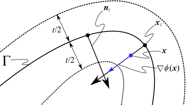
Figure 1: Tubular neighborhood of $\Gamma$ defined by the dashed line. The surface is said to be sufficiently smooth when the normal vectors $\nabla\phi(\bm{x}_{\Gamma})$ do not intersect within the tubular neighborhood, in other words each point $\bm{x}$ in this neighborhood has an unique closest point $\bm{p}(\bm{x})$ to $\Gamma$.

The surface gradient $\nabla_{\Gamma}$ on $\Gamma$ is defined by

$$\nabla_{\Gamma}u=\bm{P}_{\Gamma}\nabla u^{e},$$ (2)

where $\nabla$ denotes the full $\mathbb{R}^{3}$ gradient and $\bm{P}_{\Gamma}=\bm{P}_{\Gamma}(\bm{x})$ the orthogonal projection of $\mathbb{R}^{3}$ onto the tangential plane of $\Gamma$ at $\bm{x}\in\Gamma$ given by

$$\bm{P}_{\Gamma}=\bm{I}-\bm{n}\otimes\bm{n},$$ (3)

where $\bm{I}$ is the identity matrix. It is readily shown that the tangential gradient (2) is independent of the extension $u^{e}$ (see, e.g., [8, Chapter 9, Section 5]), hence no distinction will be made between functions on $\Gamma$ and their extensions in what follows.

The surface gradient and its components are denoted by

$$\nabla_{\Gamma}u=:\left(\frac{\partial u}{\partial x_{\Gamma}},\frac{\partial u}{\partial y_{\Gamma}},\frac{\partial u}{\partial z_{\Gamma}}\right).$$ (4)

The tangential Jacobian matrix for a vector valued function $\bm{v}(\bm{x})$ is defined as the dyadic product of $\nabla_{\Gamma}$ and $\bm{v}$,

$$(\nabla_{\Gamma}\otimes\bm{v})^{\mathsf{T}}:=\begin{bmatrix}\dfrac{\partial v_{1}}{\partial x_{\Gamma}}&\dfrac{\partial v_{1}}{\partial y_{\Gamma}}&\dfrac{\partial v_{1}}{\partial z_{\Gamma}}\\ \dfrac{\partial v_{2}}{\partial x_{\Gamma}}&\dfrac{\partial v_{2}}{\partial y_{\Gamma}}&\dfrac{\partial v_{2}}{\partial z_{\Gamma}}\\ \dfrac{\partial v_{3}}{\partial x_{\Gamma}}&\dfrac{\partial v_{3}}{\partial y_{\Gamma}}&\dfrac{\partial v_{3}}{\partial z_{\Gamma}}\end{bmatrix},$$ (5)

and the surface divergence is $\nabla_{\Gamma}\cdot\bm{v}:=\mathrm{tr}(\nabla_{\Gamma}\otimes\bm{v})$. For the vector valued function $\bm{u}$ the surface strain tensor is defined by

$$\bm{\varepsilon}(\bm{u}):=\dfrac{1}{2}\left(\nabla_{\Gamma}\otimes\bm{u}+(\nabla_{\Gamma}\otimes\bm{u})^{\mathsf{T}}\right)$$ (6)

and the in-plane strain tensor is defined by

$$\bm{\varepsilon}_{\Gamma}(\bm{u}):=\bm{P}_{\Gamma}\bm{\varepsilon}(\bm{u})\bm{P}_{\Gamma}.$$ (7)

2.2 The membrane model

Following [14, 6], we consider the problem of finding $\bm{u}:\Gamma\rightarrow\mathbb{R}^{3}$ such that

$$-\nabla_{\Gamma}\cdot\bm{\sigma}_{\Gamma}(\bm{u})=\bm{f} \quad\text{on }\Gamma,$$ (8)

$$\bm{\sigma}_{\Gamma}=2\mu\bm{\varepsilon}_{\Gamma}+\lambda\text{tr}(\bm{\varepsilon}_{\Gamma})\bm{P}_{\Gamma} \quad\text{on }\Gamma,$$

$$\bm{u}=0 \quad\text{on }\partial\Gamma_{D},$$

$$\bm{\sigma}\cdot\bm{n}=0 \quad\text{on }\partial\Gamma_{N},$$

where $\bm{f}:\Gamma\rightarrow\mathbb{R}^{3}$ is an area load,

$$\mu:=\dfrac{E}{2(1+\nu)},\quad\lambda:=\dfrac{E\nu}{1-\nu^{2}}$$ (9)

are the Lamé parameters in plane stress where $E$ denotes the Young’s modulus and $\nu$ Poisson’s ratio. Under the assumption that the material obeys Hooke’s law under plane stress, these equations can be derived from the minimization of the surface potential energy equation

$$\Pi_{\Gamma}(\bm{u}):=\dfrac{1}{2}\int_{\Gamma}\bm{\sigma}_{\Gamma}(\bm{u}):\bm{\varepsilon}_{\Gamma}(\bm{u})d\Gamma-\int_{\Gamma}\bm{f}\cdot\bm{u}d\Gamma$$ (10)

as shown in [6]. The weak form of (8) is defined by: find $\bm{u}\in V$ such that

$$a(\bm{u},\bm{v})=l(\bm{v}),\ \forall\bm{v}\in V,$$ (11)

where

$$a(\bm{u},\bm{v}) =\left(2\mu\bm{\varepsilon}_{\Gamma}(\bm{u}),\bm{\varepsilon}_{\Gamma}(\bm{v})\right)_{\Gamma}+\left(\lambda\nabla_{\Gamma}\cdot\bm{u},\nabla_{\Gamma}\cdot\bm{v}\right)_{\Gamma}$$

$$=\left(2\mu\bm{\varepsilon}(\bm{u}),\bm{\varepsilon}(\bm{v})\right)_{\Gamma}-\left(4\mu\bm{\varepsilon}(\bm{u})\cdot\bm{n},\bm{\varepsilon}(\bm{v})\cdot\bm{n}\right)_{\Gamma}+\left(\lambda\nabla_{\Gamma}\cdot\bm{u},\nabla_{\Gamma}\cdot\bm{v}\right)_{\Gamma},$$

$$l(\bm{v})=(\bm{f},\bm{v})_{\Gamma},$$ (12)

and

$$(\bm{v},\bm{w})_{\Gamma}=\int_{\Gamma}\bm{v}\cdot\bm{w}d\Gamma,\quad\text{and}\quad\left(\bm{\varepsilon}_{\Gamma}(\bm{v}),\bm{\varepsilon}_{\Gamma}(\bm{w})\right)_{\Gamma}=\int_{\Gamma}\bm{\varepsilon}_{\Gamma}(\bm{v}):\bm{\varepsilon}_{\Gamma}(\bm{w})d\Gamma$$ (13)

are the $L_{2}$ inner products.

2.3 The trace finite element method

This section describes the discretization using TraceFEM. Let $\tilde{\mathcal{K}}_{h}$ denote a quasi uniform mesh into shape regular tetrahedra of a domain $\Omega$ in $\mathbb{R}^{3}$ completely containing $\Gamma$. In this work we define the surface $\Gamma$ implicitly by constructing a signed continuous scalar distance function $\phi(\bm{x})$ such that

$$\Gamma=\{\bm{x}\in\Omega:\phi(\bm{x})=0\},$$ (14)

which is a continuous zero-isosurface. It should be noted that the property $|\nabla\phi|=1$ does not need to hold in general, i.e., it is not necessary for $\phi$ to be a distance function in the actual computations; however, if it holds, then the zero-isosurface becomes less sensitive to small perturbations. It can also be beneficial in cases of evolving surfaces, cf. [5].

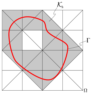
(a)

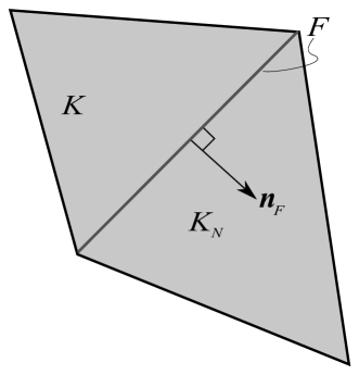
(b)

Figure 2: a) Active background mesh $\mathcal{K}_{h}$. b) Interior face $F$ shared by two active background elements $K$ and $K_{N}$.

The active background mesh is defined as the set of background elements that are cut by the zero-isosurface by

$$\mathcal{K}_{h}=\{K\in\tilde{\mathcal{K}}_{h}:\tilde{\mathcal{K}}_{h}\cap\Gamma\neq\emptyset\}$$ (15)

and its set of interior faces by

$$\mathcal{F}_{h}=\{F=K\cap K_{N}:K,K_{N}\in\mathcal{K}_{h}\}.$$ (16)

For all active cut elements $K\in\mathcal{K}_{h}$ there is a neighbor $K_{N}\in\mathcal{K}_{h}$ such that $K$ and $K_{N}$ share a face, see Figure 2.

Let $\partial\Omega_{h,D}$ denote the boundary of discrete domain $\Omega_{h}$ that is intersected by the discrete surface boundary denoted as $\partial\Gamma_{h,D}$. The finite element space is then defined by

$$V_{h}=\left\{\bm{v}\in[\tilde{V}_{h}|_{\Omega_{h}}]^{3}:\bm{v}=\bm{0}\text{ on }\partial\Omega_{h,D}\right\}$$ (17)

where $\tilde{V}_{h}$ is a space of continuous polynomials of order $m_{B}=\{1,2\}$ (subscript $B$ denotes the bulk) defined on $\tilde{\mathcal{K}}_{h}$. In this work, zero boundary conditions are treated by assuming that $\partial\Omega_{h,D}$ intersects $\partial\Omega_{h}$, which is accomplished simply by prescribing the displacements in the nodes of the background mesh. For a more general handling of boundary conditions we could use Nitsche’s method, see, e.g., [1, 17].

The finite element method on $\Gamma_{h}$ is given by: find $\bm{u}_{h}\in V_{h}$ such that

$$A_{h}(\bm{u}_{h},\bm{v})=l_{h}(\bm{v})\ \forall\bm{v}\in V_{h},$$ (18)

where the bilinear form $A_{h}(\cdot,\cdot)$ is defined by

$$A_{h}(\bm{u}_{h},\bm{v}):=a_{h}(\bm{v},\bm{w})+$$

$$\begin{cases}\gamma j_{h,1}(\bm{v},\bm{w})&\text{if }m_{B}=1\\ \gamma_{1}j_{h,1}(\bm{v},\bm{w})+\gamma_{2}j_{h,2}(\bm{v},\bm{w})&\text{if }m_{B}=2\end{cases}$$

$$\forall\bm{v},\bm{w}\in V_{h}$$

with

$$a_{h}(\bm{v},\bm{w})=\left(2\mu\bm{\varepsilon}_{\Gamma_{h}}(\bm{v}),\bm{\varepsilon}_{\Gamma_{h}}(\bm{w})\right)_{\Gamma_{h}}+\left(\lambda\nabla_{\Gamma_{h}}\cdot\bm{v},\nabla_{\Gamma_{h}}\cdot\bm{w}\right)_{\Gamma_{h}},$$ (19)

$$j_{h,1}(\bm{v},\bm{w})=\sum_{F\in\mathcal{F}_{h}}\left(\left[\nabla\bm{v}\right],\left[\nabla\bm{w}\right]\right)_{F},$$ (20)

and

$$j_{h,2}(\bm{v},\bm{w})=\sum_{F\in\mathcal{F}_{h}}h^{2}\left(\left[\nabla^{2}\bm{v}\right],\left[\nabla^{2}\bm{w}\right]\right)_{F}.$$ (21)

Here $j_{h}(\cdot,\cdot)$ denotes the face stabilization term, where

$$[\nabla\bm{v}]=\nabla\bm{v}|_{K_{i}\bigcap F}-\nabla\bm{v}|_{K_{j}\bigcap F}$$ (22)

and

$$[\nabla^{2}\bm{v}]=\nabla^{2}\bm{v}|_{K_{i}\bigcap F}-\nabla^{2}\bm{v}|_{K_{j}\bigcap F}$$ (23)

denotes the jump of $\nabla\bm{v}$ and $\nabla^{2}\bm{v}$ respectively across $F$ and $\gamma$, $\gamma_{1}$ and $\gamma_{2}$ are scalar stabilization parameters that are user defined. The discrete surface gradients are defined using the normals to the discrete surface

$$\nabla_{\Gamma_{h}}\bm{v}=\bm{P}_{\Gamma_{h}}\nabla\bm{v}=(\bm{I}-\bm{n}_{h}\otimes\bm{n}_{h})\nabla\bm{v},$$ (24)

and the right hand side is given by

$$l_{h}(\bm{v})=(\bm{f},\bm{v})_{\Gamma_{h}}.$$ (25)

The face stabilization term $j_{h}(\cdot,\cdot)$ is used to reduce ill-conditioning in $a_{h}(\cdot,\cdot)$, which results from the surface arbitrary cutting through the background elements. The discrete normals in case of $m>1$ are given by

$$\bm{n}_{h}:=\dfrac{\dfrac{\partial\bm{x}_{\Gamma_{h}}}{\partial r}\times\dfrac{\partial\bm{x}_{\Gamma_{h}}}{\partial s}}{\left|\dfrac{\partial\bm{x}_{\Gamma_{h}}}{\partial r}\times\dfrac{\partial\bm{x}_{\Gamma_{h}}}{\partial s}\right|},$$ (26)

where $\frac{\partial\bm{x}_{\Gamma_{h}}}{\partial r}$ is defined using a parametric map $\bm{F}:(r,s)\rightarrow(x,y,z)$ on a reference 2D element $T^{r}$. Details on how to compute $\Gamma_{h}$ are given in Section 3.

3 Zero-level surface reconstruction

In this section we describe the approach for extracting the discrete zero-level set $\Gamma_{h}$ from a signed distance function $\phi(\bm{x})$. The basic idea is to determine the zero-level set for each element $K$ by some form of root finding. In previous works [5, 6, 16, 1] this was done by simple linear interpolation on linear tetrahedral element. In these cases, the value of $\phi$ is exact in the nodes of $K$ and the zero-level set $\Gamma_{h}$ is interpolated linearly along the edges of $K$ yielding the corners of a planar surface element $T$. Here, however, we need to find the zero-level points along the edges of a second order tetrahedral element $K$ and the zero-level points that lie on the faces of $K$, see Figure 3. The set of these surface points will define the nodes of a second order surface Lagrange element. Since $K$ is a second order tetrahedral element, which is assumed to be affine, the arbitrary intersection with a surface will yield two types of surface elements; second order triangles and second order quadrilaterals, see Figure 4. In general, a continuous $\phi(\bm{x})$ might not be known, instead we may only have access to a discrete signed distance function $\bm{\Phi}$ defined in the nodes of $K$. In this case we can create an approximation of $\phi$using of the basis functions of the bulk element $K$:

$$\phi_{h}(\bm{x})=\sum_{i\in N_{K}}\varphi_{i}^{m_{B}}(\bm{x})\Phi_{i},$$ (27)

where $N_{K}$ is the set of nodes in $K$, $\Phi_{i}$ are the known nodal values of the signed distance function and $\varphi_{i}^{m_{B}}(\bm{x})$ is the basis function of polynomial order $m_{B}=\{1,2\}$ acting on element $K$. Note that the basis functions can alternatively be mapped or defined in the physical coordinate system since the bulk element is assumed affine.

Figure 3: Isocontours of the continuous signed distance function $\phi$ on a 10-noded tetrahedral element.

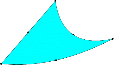
(a)

(b)

Figure 4: Resulting surface types from cutting a tetrahedral element arbitrarily with a zero-level set. (a) 6 extracted surface points mapped to a $P_{2}$ triangle element. (b) 8 extracted surface points mapped to a 8-noded serendipity element.

3.1 Root finding

Following the recent work done in [12, 11] we set up methods for extracting the zero-level set from both the continuous level set function $\phi(\bm{x})$ (if available) and the discrete $\bm{\Phi}$ (which can always be available in the nodes of the background mesh). We begin by denoting the two discrete zero-level sets

$$\Gamma_{h}|_{\phi}=\{\bm{x}\in\Omega:\Pi_{h}^{m_{\Gamma}}\phi(\bm{x})=0\},$$ (28)

$$\Gamma_{h}|_{\phi_{h}}=\{\bm{x}\in\Omega:\Pi_{h}^{m_{\Gamma}}\phi_{h}(\bm{x})=0\},$$ (29)

where the interpolant $\Pi_{h}^{m_{\Gamma}}$ of order $m_{\Gamma}$ is described presently.

3.1.1 Valid topology

As is pointed out in [12], comparing the different signs of the function $\bm{\Phi}|_{K}$ in the corner nodes of the element $K$ is not sufficient to determine if the surface topology is valid. Here a valid topology means that the arbitrary intersection of an implicit surface with the faces of a background element result in a number of surface points that can be mapped to polygons. To determine if an element is cut we compute

$$\underset{i\in N_{\mathrm{grid}}}{\min}\left(\Phi_{i}^{\mathrm{grid}}\right)\cdot\underset{i\in N_{\mathrm{grid}}}{\max}\left(\Phi_{i}^{\mathrm{grid}}\right)<0,$$ (30)

where

$$\Phi_{j}^{\mathrm{grid}}=\sum_{i=1}\varphi_{i}^{m_{B}}\left(\bm{r}_{j}^{\mathrm{grid}}\right)\cdot\Phi_{i}\quad\forall j\in N_{\mathrm{grid}},$$ (31)

$\bm{r}_{j}^{\mathrm{grid}}$ denotes a number of uniformly spaced sample points in the parametric space, see Figure 5. Note that $\varphi_{i}^{m_{B}}\left(\bm{r}_{j}^{\mathrm{grid}}\right)$ can be computed in a pre-processing step, and re-used for every background element. For an example of bad topology see Figure 5. In the case described in Figure 5d we identify high curvature by

$$\nabla\bar{\Phi}^{\mathrm{grid}}\cdot\nabla\Phi_{j}^{\mathrm{grid}}<tol,$$ (32)

where $\nabla\bar{\Phi}^{\mathrm{grid}}$ denotes the average of all $\nabla\Phi_{j}^{\mathrm{grid}}$ for all $j\in N_{\mathrm{grid}}$ and $tol$ is a user defined number chosen such that large differences in the angle between $\nabla\bar{\Phi}^{\mathrm{grid}}$ and $\nabla\Phi_{j}^{\mathrm{grid}}$ define high curvature, here $\nabla\Phi_{j}^{\mathrm{grid}}$ is given by

$$\nabla\Phi_{j}^{\mathrm{grid}}=\sum_{i=1}\nabla\varphi_{i}^{m_{B}}\left(\bm{r}_{j}^{\mathrm{grid}}\right)\cdot\Phi_{i}.$$ (33)

To be certain that the surface topology is valid we check the following conditions on each face of the tetrahedral:

• Each edge of the face may only be cut once.

• The number of cuts per face must be two.

• If no face is cut, then all nodes of the tetrahedron must have the same sign and thus the whole tetrahedron is uncut.

In case of invalid topology, local refinement can be used to resolve the background mesh.

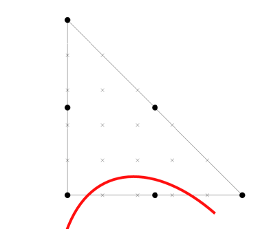
(a)

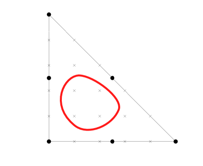
(b)

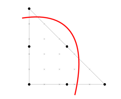
(c)

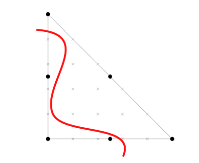
(d)

Figure 5: Examples of bad topologies visualized on side-views of a 3D parametric second order tetrahedral element with uniformly distributed sample points. The red curves represent a surface. a) One edge cut more than once. b) A small interface exists inside an element. c) More than two edges are cut. d) The curvature of the cut is too high.

3.1.2 The case of discrete level set function

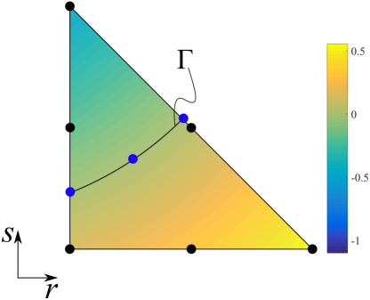
Figure 6: Isocontours of the distance function $\phi$ on a mapped face of a tetrahedral element.

In order to find the roots for $\phi_{h}(\bm{x})=0$, when $\phi_{h}(\bm{x})$ is interpolated using an interpolant $\Pi_{h}^{m_{\Gamma}}$ of order $m_{\Gamma}=2$, we follow the work done in [12, 11] using the following steps:

1. For each element check if the topology is valid by following the steps in the previous Section 3.1.1.

2. For each face $F$ of tetrahedral element $K$ in $\mathcal{K}_{h}|_{m_{B}=2}$ the nodal values of $\bm{\Phi}|_{F}$ are mapped to a parametric triangle $T^{\text{r}}|_{m_{\Gamma}=2}$, see Figure 6. If element $K$ has a valid topology it’s faces must have either two or zero cut edges, additionally at least three faces must be cut. We determine if the face is cut and which edges are cut by following a procedure analogues to (30). Additionally we renumber the nodes of the faces such that they are unique, i.e., the normal of each face $F_{K_{i}\cap K_{j}}$, no matter which tetrahedral they belong to, points in the same direction, $\bm{n}|_{F_{K_{i}\cap K_{j}}}=\bm{n}|_{F_{K_{j}\cap K_{i}}}$. This ensures that the gradients computed with the shape functions of the face elements are the same for both elements $K_{i}$ and $K_{j}$, otherwise the edge-points of the surface elements might not coincide, see Figure 7. The resulting surface is thus guarantied to be $C_{0}$ continuous.

3. On each cut edge on the parametric face $T_{m_{\Gamma}}^{r}$ we employ a Newton-Raphson iterative search scheme:
   

   $$\bm{r}_{i+1}=\bm{r}_{i}-\dfrac{\phi_{h}(\bm{r}_{i})}{\nabla\phi_{h}(\bm{r}_{i})\cdot\bm{s}}\bm{s},$$ (34)

   where $\bm{r}=[r,s]$ is the local coordinate of the parametric triangle, $\nabla\phi_{h}(\bm{r}_{i})$ is evaluated by interpolation using the basis functions and $\bm{s}$ is the search direction. To find the root along the edges, $\bm{s}$ is simply the directional vector along the edge.

4. Once the two edge points are found the inner node needs to be determined by the same root finding scheme. It turns out that the search direction is critical for the convergence of the Newton search as well as the geometrical convergence as shown in [12, 11], where the authors propose five different variations of the search directions and two ways of starting position of the search. Choosing a linearly interpolated starting position (straight line between the edge roots) and set the search direction to be the normal to the line or $\bm{s}=\nabla\phi_{h}(\bm{r}_{0})$ yields satisfying results with respect to accuracy and performance, see [11]. In some rare cases when the Newton search fails if gets stuck in a false root lying outside of the triangle, in this case we employ bisection in order to get back inside the triangle where the Newton search is continued until convergence. This approach yields a robust method in all cases but increases the number of iterations slightly for these rare cases.

5. The resulting surface points need to be numbered such that their normal is oriented in the same general direction as $\nabla\bar{\Phi}^{\mathrm{grid}}$.

6. Using this method we either get 6 surface points which are mapped to a second order triangular element, or 8 points in which case we map them to an 8-noded serendipity element. In the case of quadrilaterals the reason for mapping to an 8-noded serendipity element is to avoid the additional iterative search for the midpoint. Our argument against splitting it into two triangles is that we get less integration points which makes integration less expensive compared to two triangular elements.

7. If the resulting discrete surface needs to be used for smooth surface shading, then an additional step is needed to create a connectivity from the list of unconnected surface elements. In order to accomplish this efficiently the background mesh information for each surface patch is used to uniquely number the nodes and create the connectivity list. Note that this step is not necessary for integration.

If we have access to the exact function $\phi$, the procedure above is still valid, with the difference that we need to map $\bm{r}_{i}$ to $\bm{x}$ before evaluating $\phi(\bm{x}(\bm{r}_{i}))$ and $\nabla\phi(\bm{x}(\bm{r}_{i}))$.

It is possible to create the above scheme in physical coordinates by evaluating the basis functions in physical coordinates, $\varphi(\bm{x})$, see the Appendix. The search for roots on edges in this case is the same as above, the search on faces however is “free” since $\bm{s}=\nabla\phi(\bm{x}_{0})$. In this case we restrict $\bm{s}$ to the (planar) face of the tetrahedron by tangential projection:

$$\bm{s}=\bm{P}_{F}\nabla\phi(\bm{x}_{0}),$$ (35)

where $\bm{P}_{F}=\bm{I}-\bm{n}_{F}\otimes\bm{n}_{F}$, $\bm{I}$ is the identity matrix and $\bm{n}_{F}\otimes\bm{n}_{F}$ the outer product of the face normal to the tetrahedron face, see Figure 8. Note that the construction of $\bm{\varphi}(\bm{x})$ is done to avoid the mapping of $\bm{r}$ to $\bm{x}$ in each step of the root finding algorithm.

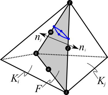
(a)

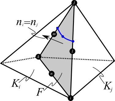
(b)

Figure 7: Face numbering. (a) $F_{K_{i}}=\{i,j,k,l,m,n\}$, $F_{K_{j}}=\{i,k,j,n,m,l\}$. (b) $F_{K_{i}}=F_{K_{j}}=\{i,j,k,l,m,n\}$.

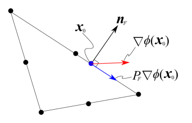
Figure 8: Sideview of a tetrahedral element. The search direction $\nabla\phi$ is projected onto the tetrahedral face $f$ (shown here as a line) resulting in a modified Newton method with the search direction $P_{F}\nabla\phi$.

4 Numerical Results

The mesh size parameter for subsequent convergence studies is defined as

$$h:=\dfrac{1}{\sqrt[3]{\mathrm{N}}},$$ (36)

where $\mathrm{N}$ is the number of nodes in the uniformly refined mesh $\mathcal{K}_{h}.$ We denote the order of the surface elements as $m_{\Gamma}$ and the order of the bulk elements as $m_{B}$. In the tables the columns named “Rate” denote the rate of convergence.

The resulting reconstructed surfaces can be seen in Figure 9.

(a) $\Gamma_{h}|_{\phi}$

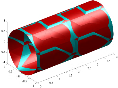
(b) $\Gamma_{h}|_{\phi_{h}}$

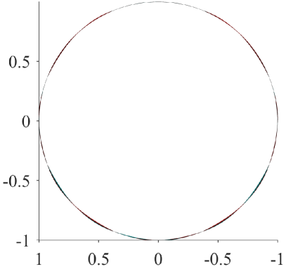
(c) Front view. $\Gamma_{h}|_{\phi}$

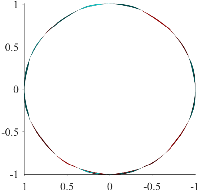
(d) Front view. $\Gamma_{h}|_{\phi_{h}}$

Figure 9: Reconstructed surface with $m_{B}=2$.

4.1 Membrane error comparison

We use the same example used in [6, 14]. A cylinder membrane with a radius $r=1$, thickness $t=0.01$ and length $L=4$, with open ends at $x=0$, $x=L$, with fixed axial displacements at $x=0$ and radial at $x=L$ and carrying an axial surface load per unit area

$$f(x,y,z)=\dfrac{Fx}{2\pi rL^{2}},$$ (37)

where $F=1$ has the unit of force. The material properties are $E=100$, $\nu=1/2$. The axial stress is given by

$$\sigma_{e}=\dfrac{F\left(1-(x/L)^{2}\right)}{4\pi rt}$$ (38)

and in the tables and figures $\sigma_{a}$ denotes the approximative stress computed by

$$\sigma_{a}:=|\bm{\sigma}_{\Gamma,a}|,\quad\bm{\sigma}_{\Gamma,a}:=[\sigma_{x_{\Gamma}},\sigma_{y_{\Gamma}},\sigma_{z_{\Gamma}}],$$ (39)

where $\sigma_{x_{\Gamma}}$, $\sigma_{y_{\Gamma}}$ and $\sigma_{z_{\Gamma}}$ are the eigenvalues to $\bm{\sigma}_{\Gamma}$. The stress error is given by

$$\epsilon_{\sigma}=\|\sigma_{e}-\sigma_{a}\|_{L_{2}(\Gamma_{h})},$$ (40)

see Figure 10 for the stress error convergence. The solution fields using a second order interpolant can be seen in Figure 11.

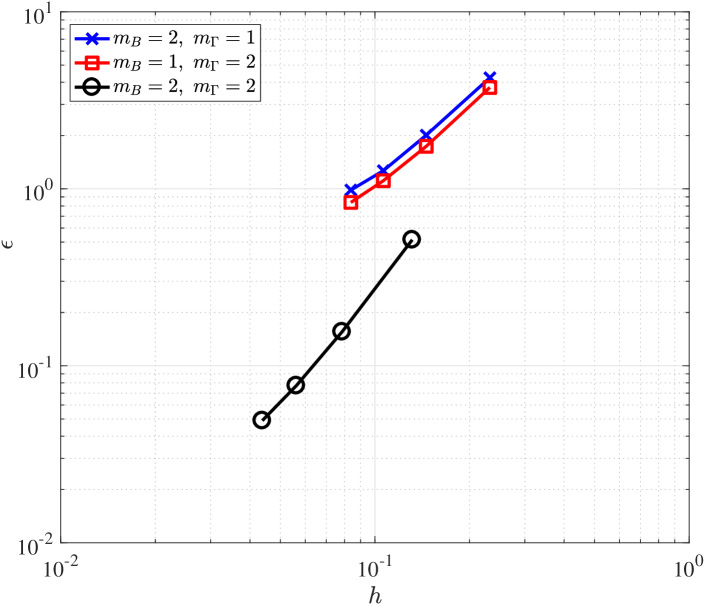
Figure 10: Stress error convergence for different surface and bulk orders.

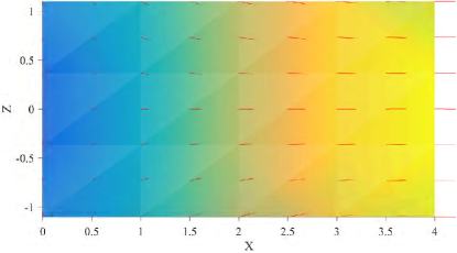
(a)

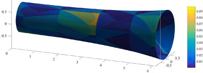
(b)

Figure 11: Membrane solution with $m_{B}=2$, $m_{\Gamma}=2$. a) On the background mesh, side view. The color field represents the resultant of the displacements. b) Solution interpolated to the surface where the color field represents the stress error $\epsilon_{\sigma}$.

4.2 Error as a function of the stability factor

In order to investigate the relation between membrane error and stabilization factor, we employ two different optimization algorithms. In the first case where $m_{B}=2$, $m_{\Gamma}=2$ in which we have $j_{h}(\bm{v},\bm{w})=\gamma_{1}j_{h,1}(\bm{v},\bm{w})+\gamma_{2}j_{h,2}(\bm{v},\bm{w})$ the minimization problem is defined as

$$\mathbb{P}_{1}=\begin{cases}\min&\epsilon(\gamma_{1},\gamma_{2})\\ \mathrm{s.t.}&0\leq\gamma_{1}<\infty\\ &0\leq\gamma_{2}<\infty\end{cases}.$$ (41)

The starting point for the minimization using the simplex algorithm [18] is $\bm{\gamma}_{0}=[1,1]$.

In case of $m_{B}=1$, $m_{\Gamma}=1$ and $m_{B}=1$, $m_{\Gamma}=2$ we have $j_{h}(\bm{v},\bm{w})=\gamma j_{h}(\bm{v},\bm{w})$ and define the minimization problem as

$$\mathbb{P}_{2}=\begin{cases}\min&\epsilon(\gamma)\\ \mathrm{s.t.}&0\leq\gamma\leq 100\end{cases}.$$ (42)

This problem is solved using the golden search method. In both optimization problems, the optimal parameter is denoted with the superscript $*$. The results of this study can be seen in Table 1 to Table 3 and Figure 12 to Figure 17. Note that although the solution with $m_{B}=1$, $m_{\Gamma}=2$ is stable without any stabilization, the interpolation of $U$ onto $\Gamma_{h}$ is not, see Figure 18.

$k$	$h$	$\epsilon_{\sigma}$	Rate	$\gamma_{1}^{*}$
1	0.2321	4.2421	-	1.4332
2	0.1456	2.0101	1.6017	0.5107
3	0.1063	1.2655	1.4708	0.5440
4	0.0838	0.9838	1.0587	1.0801

Table 1: Error convergence for the membrane with $m_{B}=1$, $m_{\Gamma}=1$

$k$	$h$	$\epsilon_{\sigma}$	Rate	$\gamma_{1}^{*}$
1	0.2321	3.7366	-	0
2	0.1456	1.7383	1.6411	0
3	0.1063	1.1108	1.4235	0
4	0.0838	0.8377	1.1864	0

Table 2: Error convergence for the membrane with $m_{B}=1$, $m_{\Gamma}=2$

$k$	$h$	$\epsilon_{\sigma}$	$\gamma_{1}^{*}$	$\gamma_{2}^{*}$	Rate
1	0.1314	0.5151	31.6944	7.8296	-
2	0.0786	0.1556	150.5121	8.4932	2.3295
3	0.0562	0.0772	137.7599	19.3374	2.0894
4	0.0438	0.0490	354.1755	21.6636	1.8235

Table 3: $\epsilon(\gamma_{1},\gamma_{2})$ for membrane with $m_{B}=2$, $m_{\Gamma}=2$

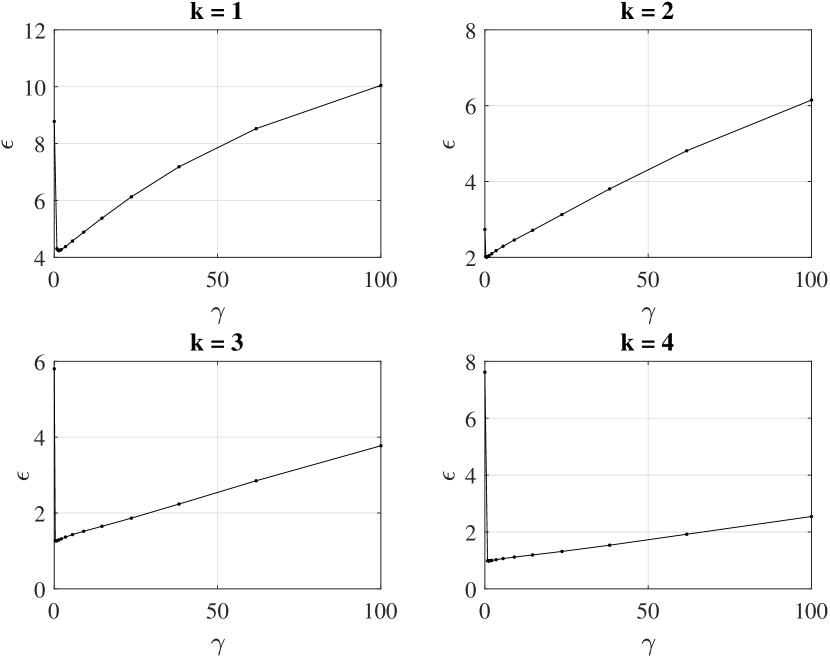
Figure 12: Stress error as a function of the stabilization factor $\gamma$ for membrane with $m_{B}=1$, $m_{\Gamma}=1$

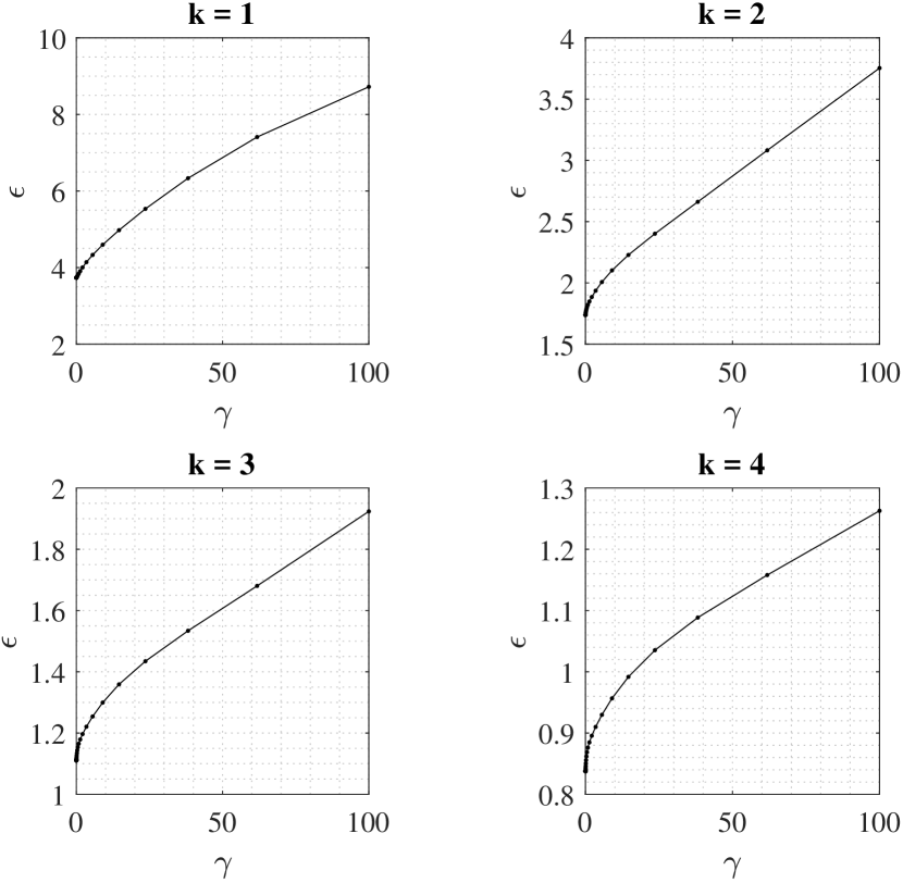
Figure 13: Stress error as a function of the stabilization factor $\gamma$ for membrane with $m_{B}=1$, $m_{\Gamma}=2$

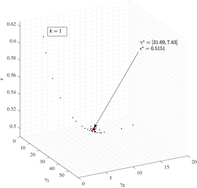
(a) 3D view

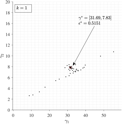
(b) $\gamma_{2}-\gamma_{1}$ view

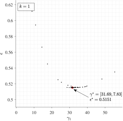
(c) $\epsilon-\gamma_{1}$ view

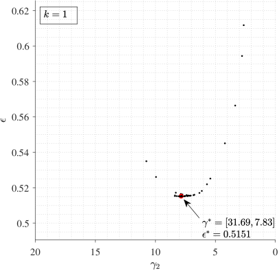
(d) $\epsilon-\gamma_{2}$ view

Figure 14: Stress error as a function of the stabilization factors $\gamma_{1}$ and $\gamma_{2}$ for membrane with $m_{B}=2$, $m_{\Gamma}=2$ and $k=1$.

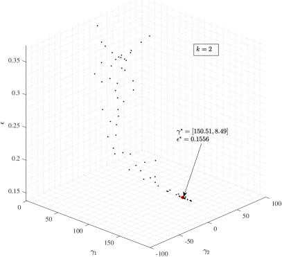
(a) 3D view

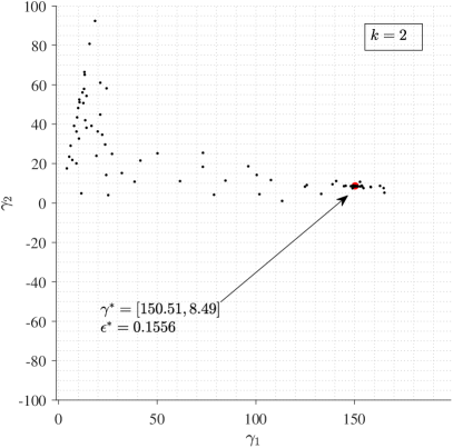
(b) $\gamma_{2}-\gamma_{1}$ view

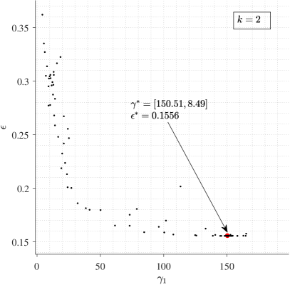
(c) $\epsilon-\gamma_{1}$ view

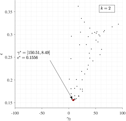
(d) $\epsilon-\gamma_{2}$ view

Figure 15: Stress error as a function of the stabilization factors $\gamma_{1}$ and $\gamma_{2}$ for membrane with $m_{B}=2$, $m_{\Gamma}=2$ and $k=2$.

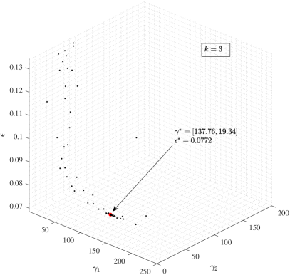
(a) 3D view

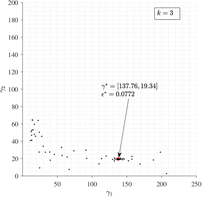
(b) $\gamma_{2}-\gamma_{1}$ view

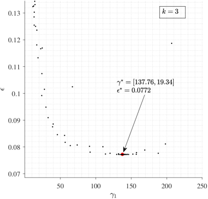
(c) $\epsilon-\gamma_{1}$ view

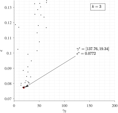
(d) $\epsilon-\gamma_{2}$ view

Figure 16: Stress error as a function of the stabilization factors $\gamma_{1}$ and $\gamma_{2}$ for membrane with $m_{B}=2$, $m_{\Gamma}=2$ and $k=3$.

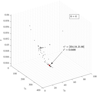
(a) 3D view

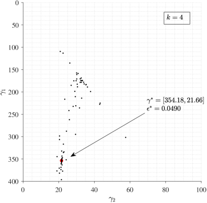
(b) $\gamma_{2}-\gamma_{1}$ view

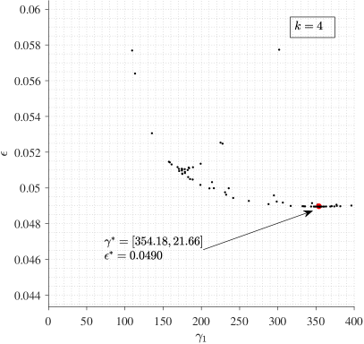
(c) $\epsilon-\gamma_{1}$ view

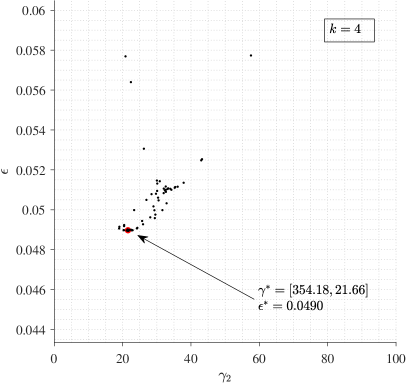
(d) $\epsilon-\gamma_{2}$ view

Figure 17: Stress error as a function of the stabilization factors $\gamma_{1}$ and $\gamma_{2}$ for membrane with $m_{B}=2$, $m_{\Gamma}=2$ and $k=4$.

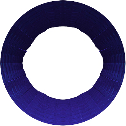
(a)

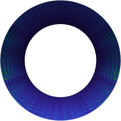
(b)

Figure 18: Displacement field (10 times enlarged) for membrane with $m_{B}=1$, $m_{\Gamma}=2$ with. (a) Front view of interpolated displacements with $\gamma=0$. (b) Front view of interpolated displacements with $\gamma=10$.

4.3 Geometrical error

In this section we numerically analyze the double approximation of $\Gamma_{h}|_{\phi_{h}}$ compared to $\Gamma_{h}|_{\phi}$ by measuring the distance error in $L_{2}$ -norm and computing the convergence rates. The geometrical error with respect to the exact and discrete distance function is given by

$$\epsilon_{\mathrm{geom}}:=\|\phi(\bm{x}_{\Gamma_{h}})\|_{L_{2}(\Gamma_{h})},$$ (43)

where $\bm{x}_{\Gamma_{h}}$ is the extracted surface using either $\phi$ or $\phi_{h}$. Another interesting aspect with respect to the tangential calculus approach is the normal errors introduced by the discrete surface approximation. The normal error with respect to the exact and discrete distance function is given by

$$\epsilon_{n}:=\|\bm{n}_{e}-\bm{n}_{a}\|_{L_{2}(\Gamma_{h})},$$ (44)

where $\bm{n}_{e}$ is the exact normal and $\bm{n}_{a}$ is the approximated evaluated either with respect to $\phi$ or $\phi_{h}$. The results can be found in Figure 19 and Tables 4 and 5.

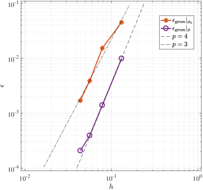
(a)

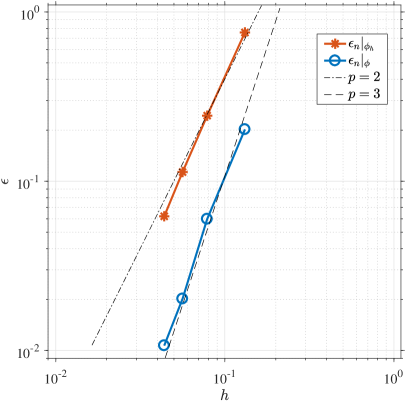
(b)

Figure 19: Geometrical errors. (a) Distance error. (b) Normals error.

$k$	$h$	$\epsilon_{\mathrm{geom}}|_{\phi}:=\|\phi(\bm{x}_{\Gamma_{h}}(\phi))\|_{L_{2}(\Gamma_{h})}$	Rate	$\epsilon_{\mathrm{geom}}|_{\phi_{h}}:=\|\phi(\bm{x}_{\Gamma_{h}}(\phi_{h}))\|_{L_{2}(\Gamma_{h})}$	Rate
1	0.1314	0.0099	-	0.0452	-
2	0.0786	0.0014	3.8065	0.0153	2.1080
3	0.0562	3.9275e-04	3.7890	0.0039	4.0747
4	0.0438	2.0799e-04	2.5500	0.0017	3.3309

Table 4: Geometrical errors comparison.

$k$	$h$	$\|\bm{n}_{e}-\bm{n}_{a}(\phi)\|_{L_{2}(\Gamma_{h})}$	Rate	$\|\bm{n}_{e}-\bm{n}_{a}(\phi_{h})\|_{L_{2}(\Gamma_{h})}$	Rate
1	0.1314	0.2023	-	0.7562	-
2	0.0786	0.0598	2.3717	0.2440	2.2012
3	0.0562	0.0202	3.2354	0.1133	2.2868
4	0.0438	0.0107	2.5491	0.0621	2.4121

Table 5: Normal errors comparison.

5 Concluding remarks

In this paper we have introduced a finite element method for higher order curved membranes using higher dimensional shape functions that are restricted to the membrane surface. We have proposed a stabilization for second order TraceFEM and show numerically that the solution is stable and converges optimally. We have compared different parameterizations and conclude that we get optimal convergence for the isoparametric case $m_{B}=2$, $m_{\Gamma}=2$. We can observe that although no solution stabilization is needed in the superparametric case of $m_{B}=1$, $m_{\Gamma}=2$, with respect to mesh convergence, we still need stabilization when interpolating the displacement field to the discrete surface, cf. Figure 18. The error difference between the case of $m_{B}=1$, $m_{\Gamma}=1$ and $m_{B}=1$, $m_{\Gamma}=2$ is fairly small, cf. Figure 10, and since we still need a second order surface reconstruction for the case of $m_{B}=1$, $m_{\Gamma}=2$, it seems natural to choose $m_{B}=2$, $m_{\Gamma}=2$ instead.

We have numerically shown the effects of different choices of the stabilization parameters $\gamma_{1}$ and $\gamma_{2}$ and conclude that the domain of optimal choices becomes bigger with smaller mesh size.

The novelty of this work is the application of face stabilization to second order TraceFEM for membrane problems. In future work we will consider higher order TraceFEM using hexahedral elements.

Appendix

Evaluation of basis functions in physical coordinates

In order to construct $\varphi(\bm{x})$ on an affine second order tetrahedron we define the geometric interpolation using the sub-parametric mapping

$$\bm{x}=\sum_{i=1}^{4}\tilde{\varphi}_{i}\bm{x}_{i}$$ (45)

where $\tilde{\varphi}_{i}$ are the basis function on the corner nodes of a 10-noded tetrahedral element, with numbering according to Figure 20, and $\bm{x}_{i}$ are the corresponding coordinates. We expand 45 and get

$$(1-r-s-t)\bm{x}_{1}+r\bm{x}_{2}+s\bm{x}_{3}+t\bm{x}_{4}=\bm{x}$$ (46)

which on matrix form is

$${\mathbf{A}\bm{r}+\bm{x}_{1}=\bm{x}}$$ (47)

where

$${\mathbf{A}=\begin{bmatrix}\bm{x}_{2}-\bm{x}_{1}&\bm{x}_{3}-\bm{x}_{1}&\bm{x}_{4}-\bm{x}_{1}\end{bmatrix}}$$ (48)

with $\bm{x}_{i}=[x_{i},y_{i},z_{i}]^{\mathsf{T}}$. We solve for $\bm{r}$ and get

$$\bm{r}(\bm{x})={\mathbf{A}^{-1}(\bm{x}-\bm{x}_{1}).}$$ (49)

Using the full basis function for the 10-noded tetrahedron $\varphi$ evaluated at $\bm{r}(\bm{x})$ we can write

$$\varphi(\bm{x})=\varphi(\bm{r}(\bm{x}))$$ (50)

and analogously

$$\nabla\varphi(\bm{x})=\nabla\varphi(\bm{r}(\bm{x})).$$ (51)

Note that for every background element $K$, ${\mathbf{A}^{-1}}$ needs only be computed once, which improves the performence of the root finding method.

Figure 20: Tetrahedral node numbering.

References

- [1] E. Burman, S. Claus, P. Hansbo, M. G. Larson, and A. Massing. Cutfem: Discretizing geometry and partial differential equations. International Journal for Numerical Methods in Engineering, 104(7):472–501, 2015.
- [2] E. Burman, D. Elfverson, P. Hansbo, M. G. Larson, and K. Larsson. Shape optimization using the cut finite element method. arXiv preprint arXiv:1611.05673, 2016.
- [3] E. Burman, P. Hansbo, and M. G. Larson. A stabilized cut finite element method for partial differential equations on surfaces: the Laplace-Beltrami operator. Computer Methods in Applied Mechanics and Engineering, 285:188–207, 2015.
- [4] E. Burman, P. Hansbo, M. G. Larson, A. Massing, and S. Zahedi. Full gradient stabilized cut finite element methods for surface partial differential equations. Computer Methods in Applied Mechanics and Engineering, 310:278–296, 2016.
- [5] M. Cenanovic, P. Hansbo, and M. G. Larson. Minimal surface computation using a finite element method on an embedded surface. International Journal for Numerical Methods in Engineering, 104(7):502–512, 2015.
- [6] M. Cenanovic, P. Hansbo, and M. G. Larson. Cut finite element modeling of linear membranes. Computer Methods in Applied Mechanics and Engineering, 310:98 – 111, 2016.
- [7] M. Delfour and J.-P. Zolésio. A boundary differential equation for thin shells. Journal of differential equations, 119(2):426–449, 1995.
- [8] M. Delfour and J.-P. Zolésio. Shapes and geometries: Metrics. Analysis, Differential Calculus, and Optimization, SIAM, Philadelphia, 2011.
- [9] G. Dziuk. Finite elements for the beltrami operator on arbitrary surfaces. In Partial differential equations and calculus of variations, pages 142–155. Springer, 1988.
- [10] G. Dziuk and C. M. Elliott. Finite element methods for surface pdes. Acta Numerica, 22:289–396, 2013.
- [11] T. Fries, S. Omerović, D. Schöllhammer, and J. Steidl. Higher-order meshing of implicit geometries - part: I integration and interpolation in cut elements. Computer Methods in Applied Mechanics and Engineering, 313:759–784, 2017.
- [12] T.-P. Fries and S. Omerović. Higher-order accurate integration of implicit geometries. International Journal for Numerical Methods in Engineering, 2015.
- [13] M. E. Gurtin and A. Ian Murdoch. A continuum theory of elastic material surfaces. Archive for Rational Mechanics and Analysis, 57(4):291–323, 1975.
- [14] P. Hansbo and M. G. Larson. Finite element modeling of a linear membrane shell problem using tangential differential calculus. Computer Methods in Applied Mechanics and Engineering, 270:1–14, 2014.
- [15] P. Hansbo, M. G. Larson, and A. Massing. A stabilized cut finite element method for the darcy problem on surfaces. arXiv preprint arXiv:1701.04719, 2017.
- [16] P. Hansbo, M. G. Larson, and S. Zahedi. Stabilized finite element approximation of the mean curvature vector on closed surfaces. SIAM Journal on Numerical Analysis, 53(4):1806–1832, 2015.
- [17] C. Lehrenfeld. A higher order isoparametric fictitious domain method for level set domains. arXiv preprint arXiv:1612.02561, 2016.
- [18] J. A. Nelder and R. Mead. A simplex method for function minimization. The Computer Journal, 7(4):308, 1965.
- [19] M. A. Olshanskii and A. Reusken. Trace finite element methods for pdes on surfaces. arXiv preprint arXiv:1612.00054, 2016.
- [20] M. A. Olshanskii, A. Reusken, and J. Grande. A finite element method for elliptic equations on surfaces. SIAM journal on numerical analysis, 47(5):3339–3358, 2009.