Fast radio burst source properties and curvature radiation model
Abstract
We use the observed properties of fast radio bursts (FRBs) and a number of general physical considerations to provide a broad-brush model for the physical properties of FRB sources and the radiation mechanism. We show that the magnetic field in the source region should be at least 1014 Gauss. This strong field is required to ensure that the electrons have sufficiently high ground state Landau energy so that particle collisions, instabilities, and strong electro-magnetic fields associated with the FRB radiation do not perturb electrons’ motion in the direction transverse to the magnetic field and destroy their coherent motion; coherence is required by the high observed brightness temperature of FRB radiation. The electric field in the source region required to sustain particle motion for a wave period is estimated to be of order 1011 esu. These requirements suggest that FRBs are produced near the surface of magnetars perhaps via forced reconnection of magnetic fields to produce episodic, repeated, outbursts. The beaming-corrected energy release in these bursts is estimated to be about ergs, whereas the total energy in the magnetic field is at least ergs. We provide a number of predictions for this model which can be tested by future observations. One of which is that short duration FRB-like bursts should exist at much higher frequencies, possibly up to optical.
keywords:
radiation mechanisms: coherent non-thermal - methods: analytical - radio: fast bursts, theory1 Introduction
Fast radio bursts (FRBs) are Jansky-level millisecond duration transient events at GHz frequencies of unknown physical origin discovered in pulsar surveys (Lorimer et al., 2007; Thornton et al., 2013). They have an all-sky rate of to above fluence (Thornton et al., 2013; Keane & Petroff, 2015; Rane et al., 2016; Champion et al., 2016). Very recently, the location of one of these bursts FRB 121102, a repeater, has been determined to an accuracy of by interferometry with the Jansky Very Large Array (Spitler et al., 2016; Scholz et al., 2016; Chatterjee et al., 2017). This FRB is found to be associated with a dwarf star-forming host galaxy at redshift z = 0.19273 (Tendulkar et al., 2017). The FRB is also associated with a persistent radio source (Chatterjee et al., 2017), and their separation is further pinned down to ( in physical distance) by the European VLBI Network (Marcote et al., 2017).
It is not surprising that the distance of FRB 121102 is Gpc considering that many observational evidences had already suggested that FRBs are at cosmological distances (see Katz, 2016a, for a brief review). First of all, their dispersion measures (the column density of free electrons along the line of sight ) are much larger than the contribution from the interstellar medium (ISM) in the Milky Way by roughly an order of magnitude111A list of all reported FRBs and their properties can be found at http://www.astronomy.swin.edu.au/pulsar/frbcat/ (Petroff et al., 2016).. Second, if the DM is mostly contributed by an ionized nebula with electron temperature , then in order to avoid free-free absorption of GHz waves the size of the nebula must be larger than (Luan & Goldreich, 2014). Moreover, the strength of H and UV continuum flux limits combined with the free-free absorption argument suggest that at least the “Lorimer burst” FRB 010724 is at a distance (Kulkarni et al., 2014).
Confirmation of the cosmological origin means that FRBs are very energetic events. If the FRB sources are isotropic (the effect of anisotropy will be included later on), then the energy release is
| (1) |
where is the fluence, is the luminosity distance and is the width of the FRB spectrum. If FRB radiation is incoherent, for burst duration , the area of the emitting region in the transverse direction — for a source with sub-relativistic speed — is , so the brightness temperature is
| (2) |
where is the peak specific flux, is the angular diameter distance (cm), is the lab-frame frequency, is speed of light, and is the Boltzmann constant; we use the convenient notation throughout the paper. Note that if the source is moving toward the Earth at Lorentz factor , then (the comoving frame temperature) is smaller by a factor of than estimated in equation (2). For any reasonable Lorentz factor, the brightness temperature exceeds the Compton catastrophe limit of K. This means that FRB radiation must be coherent and the emitting particles relativistic, as pointed out by Katz (2014).
Regarding the nature of FRBs, the major unknowns are their progenitors and radiation mechanism. Many progenitor models have been proposed, including: collapsing neutron stars (Falcke & Rezzolla, 2014; Zhang, 2014), neutron star or white dwarf mergers (Piro, 2012; Kashiyama et al., 2013; Totani, 2013), magnetar bursts222It should be noted that Tendulkar et al. (2016) failed to observe a FRB during SGR1806-20’s big outburst. (Popov & Postnov, 2010; Lyubarsky, 2014; Pen & Connor, 2015; Katz, 2016b; Murase et al., 2016), supergiant pulses from young pulsars (Connor et al., 2016; Cordes & Wasserman, 2016; Katz, 2016c; Lyutikov et al., 2016; Katz, 2016d), (Galactic) flaring stars (Loeb et al., 2014), relativistic jets running into clouds (Romero et al., 2016), asteroids colliding with neutron stars (Geng & Huang, 2015; Dai et al., 2016), close neutron star-white dwarf binaries (Gu et al., 2016), lightning in the neutron star magnetosphere (Katz, 2017), and plasma stream sweeping across the neutron star magnetosphere (Zhang, 2017). These works are only based on considerations of energetics and timescales, and the authors simply assumed that (a fraction of) the free energy available in the system is radiated away at GHz frequencies by coherent charge “patches” via e.g. curvature or synchrotron processes. However, the properties of the emitting particles/plasma and conditions for coherent emission have not been discussed in detail and will be the focus of this paper.
Cordes & Wasserman (2016) used coherent curvature radiation to explain both FRBs and the MJy shot pulses from the Crab pulsar, but the formation and stability of the relativistic near neutral coherent patches333To explain the MJy shot pulses from the Crab pulsar, the coherent patch has fractional charge (net charge divided by the total number of particles) ; particles of positive and negative charges are moving in the same direction. The basic reason for requiring an extremely small fractional charge is that the energy of FRB electromagnetic waves comes from particles’ initial kinetic energy in the model of Cordes & Wasserman (2016). The cooling time is much shorter than 1 ns (see §3) unless an amount of net charge is associated with kinetic energy . Another reason for quasi-neutrality is the electrostatic repulsion. in their model were not discussed. Ghisellini (2017) derived the general conditions for synchrotron maser emission; GHz synchrotron emission requires weak (and ordered) magnetic field ( G for electrons and G for protons) which can be found at distances from a neutron star for a dipole field configuration ; where is the Lorentz factor of particles perpendicular to the B-field. Ghisellini (2017) pointed out that the energy requirement for FRBs may be hard to satisfy for the synchrotron maser model if FRBs are at cosmological distances. In an earlier paper, Lyubarsky (2014) proposed that synchrotron maser emission may be produced when a magneto-hydrodynamic wave generated in a magnetar giant flare interacts with the surrounding pulsar wind nebula at a distance of (here ). The common problem of Ghisellini (2017) and Lyubarsky (2014) models is that they did not discuss how the particle distribution (population inversion) for efficient maser emission can be achieved.
Most FRBs models are based on neutron stars (NS), which could naturally explain their short durations, large energy requirement, ordered magnetic field (hereafter B-field) needed for coherent emission, and repetitions with intervals between to seconds (the only repeater so far is FRB 121102, but others may also be repeating, see Lu & Kumar, 2016). In this paper, we use general physical considerations to show that the B-field in the FRB source plasma should be and hence FRBs are most likely to be produced in the magnetosphere of a NS or stellar-mass black hole. We also note that the persistent radio source near FRB 121102 is consistent with being a supernova remnant (SNR) energized by a young NS/magnetar (Metzger et al., 2017; Kashiyama & Murase, 2017), although the possibility of an active galactic nuclei (AGN) cannot be ruled out (Tendulkar et al., 2017).
Much of the work presented in this paper was done in the summer of 2016, but the writing up of the paper took a long time due to some pressing matter. We have made every effort to cite papers related to this work that have been published in the meantime in this fast developing field.
In §2, we provide estimates for the size of the source region, and the strength of the electric field associated with the FRB radiation at the source. In §3, we show that coherent curvature radiation in neutron star magnetosphere can explain the FRB properties, and we also provide a number of arguments to show that the B-field strength should be G. Some predictions of this model are discussed in §4, and a summary of the main results are provided in §5.
2 General considerations
We provide a broad-brush picture of the FRB source in this section based on general physics considerations.
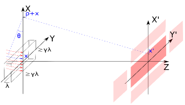
Considering that the FRB radiation is coherent, the size of the source along the line of sight cannot be larger than the wavelength () of the radiation we observe. If the source is moving toward us with a Lorentz factor , the frequency in the source frame is smaller than in the lab frame by a factor , and the transverse size corresponding to the wavelength is . Since particle velocities are , separation of along the line of sight can be maintained over a lab-frame time . The transverse source size is often taken to be . However, this need not be the case. The transverse size can be larger than by factor and still coherence can be maintained; . This is because the time delay between the arrival of photons at the observer from the opposite ends of the source in the transverse direction is smaller than provided that ; where is the angular diameter distance to the source, and is the distance between the source and the trigger point — located behind the source — from which the signal originates and propagates outward and triggers different points in the source to start radiating. For FRBs at distances , the requirement on is
| (3) |
Moreover, the shape of the coherent patch in the transverse direction is unknown. In the following, we take the area of the coherent patch in the transverse direction to be
| (4) |
where contains two multiplication factors and corresponding to the directions of the two principal axes in the transverse plane.
Thus, the maximum coherent volume in the lab frame is
| (5) |
and in the comoving frame
| (6) |
This coherent patch contributes to the FRB radiation for a time duration of order in the observer’s frame, during which the source has traveled a distance (in the lab frame) toward the observer. The patch turns off after this time and another patch lights up so that the intrinsic FRB duration is much longer than . There could be more than one coherent patches () adding up incoherently, and a continuous plasma flow could produce coherent radiation for a duration longer than ; two sources that are separated by a distance larger than the size of a coherent zone are treated as two independent patches, and even within a coherent zone we can have multiple patches if the radiation they produce is not in phase. If the same source produces coherent radiation continuously for a time duration longer than (in observer’s frame), then we tag it as a different source after time interval and yet another source after and so on.
The total isotropic equivalent of energy release for FRBs is erg and the isotropic equivalent luminosity is erg s-1 (for a cosmological distance of cm). In the far field (Fraunhofer diffraction) limit, the solid angle within which electromagnetic (EM) waves add up coherently is444 For a coherent patch with rectangular shape in the transverse direction and area , the beaming solid angle . Equation (7) is only correct in the limit and . For smaller ’s, the energy density associated with electromagnetic waves is larger than our current, conservative, estimate, because more energy is produced in a smaller coherent volume.
| (7) |
If there are distinct coherent patches, each of volume , contributing to the total observed FRB flux at any given time, the beaming corrected total energy is
| (8) |
The average lab-frame energy density in EM waves in the radiating plasma is
| (9) |
which is of order 10 erg cm-3. Therefore, the electric and magnetic field strengths associated with this EM wave energy density are
| (10) |
where the B-field strength is in Gauss. The electric field is very strong in the sense that . Thus, unless this field is almost exactly perpendicular to the local magnetic field it will accelerate electrons to highly relativistic speeds and drain the energy out of the FRB radiation.
Since all the photons from a patch must be traveling in nearly the same direction and in phase in order that their fields add coherently, we therefore infer that the electric and magnetic fields associated with the observed FRB radiation calculated above is in a direction roughly perpendicular to the patch’s velocity vector.
3 FRB source properties: coherent curvature radiation
Guided by general considerations of the last section that the B-field in the region where the observed radio photons from FRBs are produced is large, we restrict ourselves to the magnetosphere of a neutron star or a stellar-mass black hole. The curvature radiation — radiation produced when charged particles stream along curved B-field lines — is an efficient way in these conditions to produce large coherent radiation. In this section, we describe a detailed curvature radiation model that can reproduce observed FRB properties without any fine tuning of parameters.
Let us consider an electron moving with Lorentz factor along a B-field line of local curvature radius . Due to its acceleration along the B-field curvature, the electron produces EM waves at frequency
| (11) |
and the power radiated is
| (12) |
The second expression for is obtained by expressing in terms of using equation (11), i.e.
| (13) |
The electron’s radiation is beamed in the forward direction within a cone of angle , and the pulse time in the observer frame is smaller than the lab-frame time by a factor . Thus, the isotropic luminosity due to one electron, in the observer frame, is given by
| (14) |
Since we are considering radiation from a coherent patch where all electrons are moving with almost exactly the same velocity () and streaming along nearly parallel B-field lines, we can take the patch to be moving with a Lorentz factor , and electrons in the patch’s comoving frame to be essentially at rest. Let us consider that the electron density in the comoving frame is , which we express in terms of the Goldreich-Julian (GJ) density (Goldreich & Julian, 1969):
| (15) |
where
| (16) |
, and are the radius, rotation period and surface B-field strength of a neutron star, and is the distance from the coherent patch to the center of the star. The spin down time for the neutron star due to dipole radiation is
| (17) |
So if the object underlying FRBs is a neutron star with B-field strength G, then it can produce radio bursts for only a relatively short period of time of order a few hundred years. We note that the surface B-field of the FRB progenitor star may not be of dipole configuration; higher order multipole components give a smaller spin down power and hence a longer spin down time.
As our fiducial parameter, we take and use hereafter, so the total number of electrons in the patch that are radiating coherently is
| (18) |
The isotropic equivalent luminosity, in the observer frame, due to coherent patches (each containing electrons) can be calculated using equations (14) & (18)
| (19) |
or
| (20) |
In arriving at the above equation we made use of equation (13). The observed FRB isotropic luminosity is erg s-1, which can be easily accounted for if , or (or smaller values if some combination of these variables are adjusted). The beaming corrected luminosity in the lab frame is
| (21) |
| (22) |
The factor in the numerator on the RHS of equation (21) is the solid angle of the radiation beam from the patch divided by , and the factor in the denominator is the ratio of the observer frame and lab frame times.
The total kinetic energy of electrons in all radiating patches in the lab frame is
| (23) |
Combining equations (22) & (23), we find the cooling time of electrons in the lab frame
| (24) |
which is much shorter (by a factor ) than the lab frame time duration () over which the patch is radiating. This requires that there is an electric field parallel to the B-field that can accelerate electrons and sustain their Lorentz factor at for the time duration of . The required electric field in the lab frame is given by
| (25) |
We can express the electric field in terms of the FRB luminosity using equation (20)
| (26) |
This field, parallel to the B-field, is of the same order as the perpendicular electric field associated with the FRB radio emission (equation 10). The radiation can be sustained for a duration longer than in the observer’s frame provided that the electric field is maintained by some process for longer than (lab frame) such as an ongoing reconnection of B-field. In §3.2, we provide a possible magnetic reconnection geometry in which such a parallel electric field can be maintained.
The electric current associated with the motion of electrons in the volume is . The number density of particles with positive charge is nearly the same as the electron number density in order that the plasma is charge neutral. And since these positively charged particles are accelerated by the electric field in opposite direction to the electrons, the total current in the region is . Thus, the B-field generated by the current inside the patch is
| (27) |
or
| (28) |
This induced B-field is in the direction perpendicular to the primary B-field (), and the induced field lines are closed curves that lie in planes normal to . Thus the superposition of the two fields – & – will point in different directions at different locations in the source. Particles are stuck in the lowest Landau state, as shown later, and therefore their motion is along B-field lines. In order for these particles to produce coherent radiation their velocity vectors should be nearly parallel. To be more precise, the angle between the velocity vectors for different particles should not be larger than . This constraint provides a lower limit on the strength of the original B-field in the region:
| (29) |
It is unphysical that a large number of patches would turn on simultaneously on a timescale of ns, so we expect that . Moreover, is at most of order unity, as been constrained in §2 (eq. 3). This means that FRBs are most likely produced near the surface of a neutron star or the event horizon of a stellar-mass black hole in a region where the B-field strength is G.
3.1 Radio wave propagation through neutron star magnetosphere & constraint on particle density
In this sub-section we discuss effects on GHz waves as they propagate through the magnetosphere of a neutron star. The main goal is to ascertain whether radio waves can propagate through this media without suffering excessive absorption, and to provide a constraint on the particle density in the region where FRB radiation is produced. We show below that wave absorption is small as long as the particle number density () is smaller than 1018 cm-3, which is about times the GJ density, i.e. (note that and ).
Transverse electromagnetic waves produced by the curvature radiation are linearly polarized with the electric field vector () perpendicular to both the local B-field () and the wave-vector as long as , where
| (30) |
is the plasma frequency, and
| (31) |
is electron cyclotron frequency.
The condition for the propagation of transverse EM waves, with perpendicular to , in a highly magnetized plasma, is: (e.g. Arons & Barnard, 1986). Therefore, although the plasma frequency in the FRB source region is much larger than FRB radio frequency, the GHz waves can still propagate through the medium at a speed that is extremely close to .
It can be shown that as radio waves propagate through the magnetosphere with changing B-field direction, adiabatically changes its direction so that it is perpendicular to both the local & , as long as (see Cheng & Ruderman, 1979).
In other words, the polarization vector of photons is along while moving through the region of the magnetosphere where .
The column density of electrons in the source region of FRB model we have described above is cm-2 (or 300 pc cm-3). However, the contribution of the magnetosphere to the observed DM value of FRBs is negligible. This is due to the fact that the effective plasma frequency in the presence of a strong B-field is reduced by a factor of , and thus the contribution to the DM from the FRB source region is pc cm-3.
3.1.1 Free-free absorption of GHz radiation
The FRB waves propagating through the medium where they are produced are subject to the free-free absorption process, which is calculated here. The standard result for free-free absorption (e.g. Rybicki & Lightman, 1979) cannot be used for the FRB system because particle motion is restricted by the strong magnetic field and is essentially confined to one dimension. A self-consistent derivation of free-free opacity for the FRB source is presented below.
Consider Coulomb interaction between an electron () and a proton (or positron) – hereafter – moving with Lorentz factors and , respectively. These particles are streaming along strong magnetic field lines of strength , and they remain in the lowest Landau state during the entire interaction. The angle between their momentum vectors is in the lab frame. We will use the method of virtual quanta to calculate Bremsstrahlung emission and absorption, which is carried out in the rest frame of the electron (prime frame), and then transformed back to the lab frame. The Lorentz factor of and the angle between the momentum vectors in the prime frame are given by
| (32) |
where .
The x-axis is taken to be along the electron-momentum, and the x-y plane is the plane of & p+ momenta. The magnetic field in the prime frame at the location of the electron is
| (33) |
The main idea behind the virtual quanta technique is that the electromagnetic field due to in the prime frame is sharply peaked in a narrow region close to the particle. This field is Fourier decomposed and each frequency component is treated as a virtual photon that gets scattered by the electron.
The electric field components due to in the prime frame is calculated using the Liénard–Wiechert potential. We prefer to calculate the field in the rest frame and then Lorentz transform it to the prime frame followed by a rotation along the z-axis by an angle so as to obtain field components along the and axes. The component of the electric field at the location of the electron is given by
| (34) |
where
| (35) |
and is the minimum distance between and in the prime frame.
For strong field associated with the FRB model, the y-component of the electric field and the magnetic field associated with are too weak and of too small a frequency to excite the electron to a higher Landau level and therefore these fields are ignored for the Bremsstrahlung calculation. The electron motion along the x’-axis is described by
| (36) |
The electric field in the radiation zone due to the acceleration of the electron is
| (37) |
where
| (38) |
The Poynting flux due to the electron acceleration is given by
| (39) |
The energy release per unit frequency and per unit solid angle in a – scattering is
| (40) |
where
| (41) |
This integral can be carried out using the modified Bessel functions
| (42) | ||||
| (43) |
and we obtain
| (44) |
where
| (45) |
Making use of equations (39) & (44), we obtain the energy release per unit frequency and per solid angle in one – encounter
| (46) |
or
| (47) |
For a plasma with and densities of & the Bremsstrahlung emissivity is given by
| (48) |
The emission is beamed along the electron momentum vector within an angle of , and the spectrum peaks at which is a factor larger than the GHz frequency of FRBs we are interested in. Therefore, we will consider the low frequency limit where
| (49) |
is the Euler-Mascheroni constant. It can be shown that for FRBs, the term containing in the above expression for is much smaller than the term. With these approximations, we finally arrive at the following simplified expression for Bremsstrahlung emissivity
| (50) |
where is the angle between electron momentum vector and the photon, and is the angle between & momentum vectors; . The emissivity decreases very rapidly with angle for .
Finally, we can obtain the expression for free-free absorption coefficient, including correction for the stimulated emission, in Rayleigh-Jeans limit using the Kirchhoff’s law:
| (51) |
or
| (52) |
where the electron temperature along the magnetic field.
Inside the source region where the photons are moving almost parallel to electrons that produced them — — the optical depth corresponding to the source length along the line of sight is
| (53) |
where we took as per equation (13). The optical depth due to particles moving in the direction opposite to the electrons is much smaller than that given by equation (53) for a electron-positron plasma555This is due to the fact that free-free radiation produced by positrons is narrowly beamed along their momentum vector, and very little radiation comes out in the opposite direction. Absorption of photons moving head-on toward positrons, which is related to the inverse of the free-free emission, has therefore, much smaller cross-section than absorption of photons moving in the same direction as positrons. The lower cross-section more than compensates for the larger number of positrons encountered by photons while traveling the distance .. For a electron-proton plasma, the absorption of GHz photons by protons is even smaller and can be ignored.
Equation (53) suggests that the particle density within the FRB source region should not be much larger than cm-3 to avoid free-free absorption of photons. However, the allowed density is sufficient for producing the observed typical FRB luminosity of erg s-1 for a coherent source of transverse size , i.e. (see eq. 20).
Once particles leave the acceleration zone the waves might suffer significant absorption if the outside temperature is much lower than . This is, however, unlikely. The cooling time for electrons increases dramatically outside the coherence zone, and becomes of order s) (where is taken from equation 12). In this case, the electron temperature stays relativistic and the free-free absorption at GHz is small as long as the coherence zone is contained inside a somewhat larger acceleration zone. Moreover, as photons travel further out in the magnetosphere, the angle between their momentum vector and the local magnetic field direction () increases, and decreases rapidly for (as – see eq. 52) which keeps the free-free absorption small.
The free-free absorption increases with decreasing frequency as , and therefore waves with MHz are likely to be absorbed in the source region. This might explain the lack of detection of FRBs below GHz frequencies in a few cases.
The bottom line is that the GHz photons can escape the magnetosphere of a magnetar without suffering much free-free absorption provided that the plasma density in the source region cm-3. This upper limit to the density is larger than the GJ density by a factor . Moreover, the density required for our model to produce the observed luminosity of a typical FRB of erg s-1 is cm-3, and the transverse size of the source is . The contribution to the DM of a FRB from the magnetar source region is negligible due to the modification of the EM wave dispersion relation in a highly magnetized plasma ().
3.2 Energy dissipation in current sheet to power FRBs
What we have established thus far, using general arguments, is that the B-field in the region where FRB GHz radiation is produced is G, and the electric field component parallel to the B-field is esu. This electric field needs to be sustained for at least 1 s (). In this sub-section we consider one possible way that such an electric field could arise: when inclined B-field lines in the magnetosphere of a neutron star are forced to come together and reconfigure. In this process of magnetic reconnection, a fraction of the B-field energy is dissipated and charged particles are accelerated by to relativistic speeds and produce coherent curvature radiation.
The calculations presented in this sub-section are less robust than other parts of the paper because the physics of reconnection and particle acceleration are poorly understood especially when the magnetization is large ( in the FRB source region). Fortunately, the uncertainties associated with the calculation of reconnection and do not affect other parts of this paper apart from some of the predictions of our model described in §4.
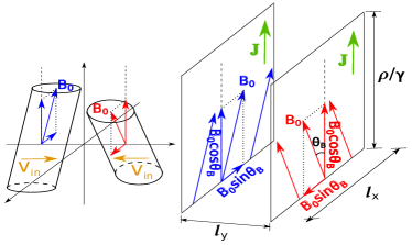
Let us consider the B-field directions at the opposite sides of the current sheet to be inclined at an angle , and B-field strength to be ; we consider rad. The B-fields on the two sides of the sheet can be decomposed as parallel and anti-parallel components (see Fig. 2). Only the anti-parallel components of the B-field, which have strengths of , are dissipated inside the current sheet, whereas the parallel components with strength (or the guide field) remain intact. Let us take the plasma speed flowing into the current sheet to be . The dimension of the current sheet along the line of sight (or along the guide field) is and in the transverse direction is . The thickness of the current sheet is . Thus, the transverse area of the coherent volume is .
The dissipation rate of magnetic energy is
| (54) |
From the cooling time argument, we require and hence
| (55) |
where we have used and . The radiation efficiency is
| (56) |
The inflow velocity is also given by , i.e.
| (57) |
The angle can be roughly estimated from the condition that ; where . Since , we find that . The system becomes charge starved for larger angles, and that would trigger rapid dissipation of magnetic fields. For , we have and hence . There is considerable flexibility (and uncertainty) in values the parameters , , and can take, and hence a wide range of efficiencies from to are allowed in the magnetic reconnection model.
The intrinsic durations of most FRBs only have upper limits , because they were not resolved after deconvolution of the scattering broadening and DM smearing resulting from the finite channel width of radio telescopes. However, the repeating events from FRB 121102 showed various observed durations (2.8-8.7 ms) with no clear evidence of scattering broadening (Spitler et al., 2016). Also, FRB 121002 showed resolved double-peaked profile with separation of about between the peaks (Champion et al., 2016). If we assume that these relatively long durations are intrinsic, the process that drives the magnetic reconnection may be relatively “slow”, i.e. operating on timescales much longer than the light-crossing time of the NS. The large scale steady state structure of the force-free NS magnetosphere (e.g. dipole or multipole with twists) can be solved (e.g. Akgün et al., 2016). However, the B-field configuration very close to the surface of a NS (most likely a magnetar for FRBs) is still poorly understood (e.g. Mereghetti, 2008), so the mechanism for forced reconnection of magnetic fields is uncertain. One possible scenario is that magnetic flux emerges from below the NS surface due to buoyancy (e.g. Muslimov & Page, 1995; Viganò & Pons, 2012) and then the emergent B-field reconnects with pre-existing B-field in the magnetosphere at some inclination. Another possibility is the slow movement of the NS crust where the field lines are anchored. For example, in the first scenario, flux emergence from under the NS surface occurs on a timescale
| (58) |
where is the depth from which the flux emerges, is mass density of the surface layer, is the Alfvén speed.
3.3 Robustness of coherent curvature radiation
In §3.3.1, we calculate the radiation field from a single particle moving along a fixed B-field line, and then we add up the contribution from particles with different Lorentz factors and moving along magnetic field lines pointing in different directions. Taking as an example, we show that the curvature radiation from different particles within a patch adds up coherently provided that (i) dispersion of the Lorentz factor of particles in the region is within a factor a few of the mean Lorentz factor (); (ii) the orientations of magnetic field lines at different points in the region are within an angle of each other; (iii) the spectrum of the emergent coherent radiation can have strong fluctuations on MHz scale; (iv) the time delay between radiation from opposite ends of the patch should be no larger than .
In §3.3.2 & 3.3.3, we discuss a number of physical effects that could perturb particle trajectories, generate or inhibit the generation of coherent bunches.
3.3.1 Condition on particle velocity and B-field orientation distributions for coherent curvature radiation
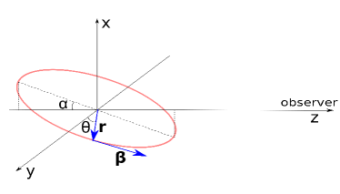
Consider a single particle with charge on a circular orbit of radius (the curvature radius of the B-field line) inclined at an angle with respect to the line of sight or axis, as shown in Fig. (3). The angular frequency is , where is the particle’s speed divided by and we assume to be constant with time in order to focus on the curvature radiation. The azimuthal angle at any retarded time is given by (we have taken for ). The electric field at the observer’s location due to the particle’s acceleration is (Rybicki & Lightman, 1979)
| (59) |
where we have used , , being the vector from the particle’s position to the observer, and we have neglected high order terms .
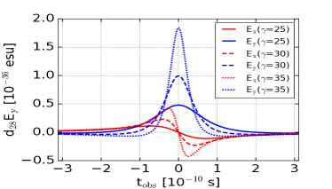
We show in Fig. (4) the x and y components of the electric field in the far field due to a single particle. Note that is anti-symmetric with and while is symmetric. If the particle flow is continuous on a timescale of , from particles with positive and negative will cancel out, but will survive. In the following, we only consider the component of , the magnitude of which is
| (60) |
where time in the observer frame is given by
| (61) |
The emission is strong only when and the duration of the emission from a single particle is .
In Fig. (5), we plot the from a coherent volume of electrons with flat distributions of Lorentz factors in the interval , orbital angles between , and azimuthal angle in the interval . We consider three different of , and radian; and three different of , , and ; where is the mean Lorentz factor. The electric field is normalized to . To get the actual electric field, one needs to multiply with the total number of electrons in the coherent patch. The general conclusion is that coherence is destroyed and the resulting electric field is much weaker when the separation of particles in a patch significantly exceeds (i.e. ) or when the direction of particle motion has a spread much larger than (i.e. ). Particle clumps with longitudinal size may be produced in various plasma instabilities, such as the two-stream instability (see §3.3.2).
We note that coherence at frequencies is unaffected if particles have a broad Lorentz factor distribution. The peak frequency of curvature radiation depends strongly on the particle Lorentz factor , so particles with Lorentz factors larger (or smaller) than 30 by a factor of more than 2 will radiate most of their energy at frequencies much above (or below) . During the reconnection, particles with a wide range of Lorentz factors may be produced, but that would not affect the observed luminosity of Jy at provided that the number of particles with Lorentz factor (e.g. between 20 and 40) is of order . We also note that FRB spectrum depends on the Lorentz factor distribution . The radiation from particles with too large Lorentz factors will be beamed away from the observer line of sight, so we expect that there should be a sharp break in the FRB spectrum somewhere above (but not too far above 10 GHz, since the chance that an observer is within the beaming cone of particles with larger Lorentz factors decreases as ).
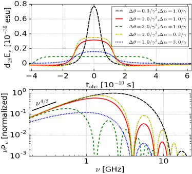
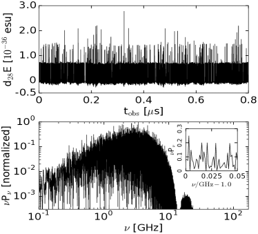
The observed FRB duration is affected by the DM smearing and broadening due to scatterings in the ISM/IGM. If the intrinsic duration of an FRB is (which is determined by the duration of magnetic reconnection), the number of coherent patches needed is ; it should be pointed out that we receive radiation from only one of these patches at a time, and the million patches are part of a semi-continuous outflow in a current sheet which we have broken up into a large number of causally connected segments for the ease of calculation. As a simple demonstration, we show in Fig. (6) the emission from 2000 identical patches that turn on and off on a timescale of (in observer frame); is taken to have the Poisson distribution with mean value . The spectrum has strong fluctuations in frequency intervals as small as MHz (Fig. 6). To model the observed FRB spectrum with rich fine-scale structure, one may need to add up contributions from different patches in more realistic ways. For example, particle flow could be episodic on s–ms timescales and different patches could have different polarizations due to the rotation of the NS or non-stationary B-field configuration. Scintillation and plasma lensing probably also play an important role in shaping the observed spectrum (e.g. Ravi et al., 2016).
The EM emission directly coming from the source region is linearly polarized, with electric field perpendicular to the primary B-field and the line of sight. Due to the rotation of the NS, and the magnetic field orientation in the current sheet changing on s timescale, the polarization angle is likely to be time dependent. The polarization state of photons can also change substantially as they propagate through plasma along the line of sight in the NS magnetosphere, magnetar wind nebula, and possibly supernova remnant. One would need to take these effects into consideration in order to model and interpret the polarization properties of FRB radiation.
3.3.2 Two stream instability in presence of electric field for relativistic relative velocity & its effect on coherent radiation
Since electrons and protons (or positrons) are accelerated by the nearly static electric field parallel to in opposite directions, the two stream instability could have an effect on the coherent radiation generation. We show that this instability could lead to the formation of particle bunches with longitudinal size on the order of on timescales much shorter than . We consider an electron-proton plasma, which is cold so that the state of the particles transverse to the B-field is in the lowest Landau level; the analysis here is applicable to electron-positron plasma as well.
Our choice of frame is such that protons are at rest in the absence of a wave, which simplifies the algebra, but does not restrict linear stability analysis. The notation in this subsection is different from the rest of the paper. We denote particle density in the fluid comoving frame without a prime (in previous sections we had used prime), and all remaining quantities are measured in the rest frame of the proton and are also denoted without a prime. Variables in the lab frame will be denoted by the subscript “lab”.
The electron and proton unperturbed densities in their comoving frames are & , and the perturbations are & respectively. The 4-velocities for electrons and protons (as measured in the comoving frame of unperturbed proton flow) are taken to be and ; . The perturbed equations for particle flux conservation follows from , and are
| (62) |
| (63) |
It follows from and (since perturbations are being carried out in the rest frame of protons) that , but . Moreover, perturbation of the equation , yields
| (64) |
We use this relation to eliminate in equation (63)
| (65) |
where , and .
The momentum equation for the cold plasma is: or ; where is the energy momentum tensor for cold plasma, is the electro-magnetic second rank tensor, is the radiation reaction force, and and are particle charge and mass. The z-component of the momentum equation is
| (66) |
The electric field is in the proton/positron comoving frame, but since particles are streaming in the direction, the -component of electric field in the lab and electron comoving frames are also . The electric force on a charged particle is balanced by the radiation reaction force, , for the unperturbed system. The perturbation to is a non-local quantity (because it depends on all the particles in the patch that are radiating coherently), and is not easy to include in the stability analysis of the system666 The effect of the radiation reaction force is likely to stabilize the system. An increase in , causes particles to be accelerated to a higher Lorentz factor, which then causes a higher radiative power output – curvature radiation power scales as (equation 12) – and the resulting higher radiation reaction force tries to restore the equilibrium state of the system.. We ignore in the perturbation analysis presented below, and due to this we might perhaps be overestimating the importance of the two-stream instability.
The perturbation of the z-component of the momentum equation for protons and electrons are:
| (67) |
and
| (68) |
Finally, it follows from the Maxwell equations that
| (69) |
Note that the density perturbation is defined in the electrons’ comoving frame, so we have the factor on the right-hand side because the equation is in the proton/positron rest frame.
Equations (62), (65), (67), (68) and (69) are five equations in five variables that we solve to determine the dispersion relation and two-stream instability growth time. Taking all perturbed variables to be proportional to , these five equations can be combined and reduced to the following two equations
| (70) |
and
| (71) |
We finally obtain the dispersion relation, which is:
| (72) |
where
| (73) |
The electron plasma frequency is
| (74) |
It should be emphasized that and are wavenumber and complex frequency in proton/positron rest frame; and are the unperturbed velocity and Lorentz factor of the electron fluid in the rest frame of proton/positron, and and are particle number densities in the rest frame of electron and proton respectively.
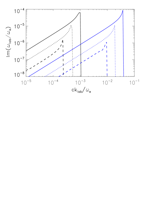
It can be shown from equation (72) that two-stream instability is present when , i.e. for sufficiently small wavenumber the system is unstable to bunching up of particles. The growth rate of instability, Im), is obtained by finding the two complex roots of equation (72), which are complex conjugates of each other. The growth rate for – and – plasma for several different values of are shown in Fig. (7). Since in equation (72) is the electron Lorentz factor as measured in the rest frame of protons, it is equal to , where and are Lorentz factors of protons and electrons measured in the lab frame.
Electron clumps of longitudinal size cm are required for the coherent curvature radiation model considered in this work. The electron density needed to generate a typical FRB luminosity of erg s-1 is cm-3 (see eq. 20 and the discussion following it — but note that in this section is same as in that equation). Therefore, rad s-1 (eq. 74). Hence, for a – plasma of (needed for the FRB curvature radiation, as per eq. 13), the clump size (, for the fastest growing mode) turns out to be cm, and the growth time for the instability is about 30 ns in the lab frame (see Fig. 7); the time required for the formation of a clump is longer (due to causality limit), and is of order s. For a – plasma, clumps of size cm also form on a timescale of s in the lab frame. Since the emission from one coherent patch lasts for 1 ns in the observer frame, which corresponds to ns in the lab frame, particle clumps form on a time scale smaller than that required for the coherent curvature radiation to operate.
We note that the electric field associated with the clumping of electrons is much weaker than estimated in equation (26) and the electric field associated with the FRB EM wave energy in equation (10). Even in the extreme case where electrons are fully separated with protons/positrons in different clumps with longitudinal separation , the electric field due to clumping is roughly given by , where is the total number of particles in one clump and is the transverse area of a coherent patch. For parameters required to produce FRB luminosities, , and , we obtain . In reality, the clumps are only partially charged and the electric field due to clumping is much smaller than this value. Therefore, the electric field associated with clumping will not be able to disperse the clumps; the back reaction of radiation on the clump can not disperse them either, because this reaction force is balanced by the reconnection electric field (eq. 26). Moreover, the electric field of charged clumps is not sufficiently strong to convert plasma waves to the EM waves at FRB luminosities.
3.3.3 Perturbation of particle trajectories by EM field and particle collisions — coherence survives
We showed in §3.3.1 that particle velocity distribution along the B-field need not be narrow for generation of coherent radiation. However, even a small dispersion in particle velocity perpendicular to the B-field can ruin the coherence. Also, the primary B-field lines along which particles in the source region are moving should be nearly parallel to each other (within an angle of ).
We show here that despite the presence of strong perpendicular electric and magnetic fields in the source region ( G; equation 28), and collision between particles with opposite charges moving relative to each other at close to the speed of light, the distribution of particle velocity perpendicular to the B-field is unaffected. The reason for this comes down to the fact that the energy of excited Landau levels are so large that particles stay in the ground state in spite of the large, time dependent, fields. And therefore, the coherence is preserved.
The energy of relativistic electrons in a magnetized medium is (see Appendix A)
| (75) |
where is the component of electron’s momentum along the B-field line, is a positive integer, and
| (76) |
is the electron cyclotron frequency. In the limit , the expression for electron energy can be approximated as
| (77) |
Thus, the energy of the electron corresponding to the lowest Landau level (for ) is
| (78) |
The plasma temperature in the direction transverse to the B-field should be cold ( keV) – even though electrons are streaming along magnetic field lines with a Lorentz factor – otherwise higher Landau levels would be populated and the emergent radiation cannot be coherent.
The motion of electrons perpendicular to the B-field is damped due to the cyclotron radiation on a very short time scale of s) (in the lab frame). So the electron velocity dispersion perpendicular to the B-field (which is proportional to the transverse temperature) should be very small unless there is a mechanism or instability that operates on a much shorter timescale and excites electrons to higher Landau levels.
From equation (75) we see that the effective electron momentum transverse to the B-field, in the first excited level (, is . This is much larger than the transverse momentum kick given to the electrons, (classically), when electrons and protons undergo Coulomb collision in the FRB source. Particle collisions, therefore, cannot dislodge electrons from their ground Landau state.
The transverse electric field associated with FRB radiation is so strong ( esu; equation 10) that it shifts the energy of the Landau levels by an amount that is much larger than . However, it can be shown that this shift is exactly the same for all Landau levels, and since is larger than the EM wave frequency ( GHz) by a factor , electrons adapt to this periodic shift in the energy levels adiabatically and remain in the ground state, i.e. the strong EM field associated with the radiation does not kill the coherence.
The B-field produced by charged particles in the source region streaming along is also strong ( G; equation 28), and its direction changes on a length scale smaller than . However, electrons adapt to this changing B-field adiabatically since the de Broglie wavelength of electrons in transverse direction, (see Appendix A), is much smaller than the curvature radius of the B-field.
3.4 Propagation of radio waves through supernova remnant
Waves generated near the surface of a relatively young NS travel through the supernova remnant left behind in the explosion that produced the NS. We show in this sub-section that the contribution to DM from the supernova remnant is nearly constant for a period of a few years as required by the data for FRB 121102 from which 17 bursts have been detected (Spitler et al., 2016; Scholz et al., 2016); this point has already been made recently by (Murase et al., 2016; Piro, 2016; Metzger et al., 2017). We also show that the optical depth of the supernova remnant for free-free absorption is small.
Let us consider that 10 of material is ejected in a supernova that produced the NS, and the initial speed of the remnant is 109 cm s-1. The particle density of the medium in the vicinity of the explosion is taken to be 10 cm-3. In this case the deceleration radius for the remnant is cm, and the deceleration time is about 200 years. The mean particle density of the ejecta yrs after the explosion is cm-3, and the electron column density is cm-2, if the ejecta is significantly ionized as suggested by Metzger et al. (2017); where yrs). Thus, the contribution of the ejecta to the FRB DM is pc cm-3. And the change to DM in three years is pc cm-3.
Seventeen radio bursts were detected from FRB 121102 in a period of 3 years, and the DM values for these events were the same (about 557 pc cm-3) during this period within the error of measurements. Thus, the age of the NS for this FRB cannot be smaller than 50 years. A similar lower limit on the age is obtained from the consideration that the DM from the host galaxy (at ) does not exceed pc cm-3 (Tendulkar et al., 2017).
The free-free absorption optical depth for the remnant at 1 GHz is ; where is the temperature of the remnant. Tendulkar et al. (2017) find for FRB 121102, and that too suggests the NS age to be 50 yrs.
It can be inferred from the large B-field strength of ( G) that the NS is most likely a magnetar. The empirical age of Galactic magnetars is to (e.g. Viganò et al., 2013), which may be taken as the upper limit of the age of the FRB progenitor.
To summarize the main result of §3, the picture that emerges is that FRB radiation is produced in a patch of comoving size , where magnetic reconnection provides the necessary electric field to accelerate charged particles to Lorentz factor , and these particles produce coherent curvature radiation. The observed FRB radiation can be produced in a small region of transverse size cm (i.e. ), with B-field strength of G, and particle density of the order Goldreich-Julian density. The reconnection of the B-field is sustained for 1 ms, and the electric field in the current sheet parallel to the primary B-field is esu.
4 Predictions of the Model
We provide in this sub-section a number of predictions of the model we have proposed for FRBs. In essence, the model is that radio waves are produced coherently in the magnetosphere of a NS with strong B-fields that undergo forced reconnection due to perhaps the movement of the neutron star crust (where the fields are anchored) or emergence of sub-surface flux tubes above the NS surface. The distortion of the B-field lines in the crust or magnetosphere builds up over a period of time, until it reaches a critical state and becomes unstable and field lines are reconfigured, dissipating a fraction of the B-field energy in a current sheet in the process. This is a well known process and is responsible for the energy release in solar flares (e.g. Shibata & Magara, 2011).
We begin by writing down the coherent curvature luminosity and the strength of the electric field parallel to the B-field in a nearly model independent form, and then specialize to magnetic reconnection to express length scales in terms of parameters appropriate for a current sheet.
| (79) |
which is essentially the same as equation (19), except that we have taken (as discussed in §3), the transverse area of the source is , and the expression for curvature radiation frequency (equation 11) has been used to eliminate the wavelength . The electric field strength () is calculated by balancing the acceleration due to electric field with the radiation back reaction force (as was done in §3 leading to equation 25) and we re-express that result as:
| (80) |
where as before is the radius of curvature of the B-field.
Thus far we have not made any reference to reconnection and current sheets, and so the above results are broadly applicable. Next, we specialize to current sheets, and make a few predictions. Since we have a rather limited first-principle understanding of the properties of current sheets and particle acceleration, the following discussion is mostly qualitative.
The thickness of the current sheet is likely to be related to the plasma frequency (), and accordingly we take ; where is a dimensionless parameter which could be of order –103 as suggested by numerical simulations (e.g. Sironi et al., 2016). Substituting for in equation (80) we find
| (81) |
which is independent of the plasma density (). Using equation (81) for , we calculate the frequency at which particles radiate most of their energy
| (82) |
and
| (83) |
The electric field , , (the angle between field lines on the opposite sides of the current sheet), and likely vary substantially from one reconnection event to another. Therefore, several general predictions can be made for FRBs according to the model described in this work.
-
1.
Electrons are likely accelerated to very different Lorentz factors in different bursts or different regions in one burst. Hence, in addition to the FRBs observed at a few GHz frequency, the model predicts that there are other FRBs that radiate at frequencies much higher than GHz (since ); some FRBs may radiate most of the energy at 10 GHz whereas others might be at Hz. Since , it is unlikely to find FRBs at frequencies much larger than Hz; this is because Hz requires esu — which is of order the Schwinger limit on electric field strength of — and fields of larger strength cannot be sustained for long as they lead to spontaneous creation of electron-positron pairs and breakdown of the vacuum. High energy photons can be produced due to a process such as the resonant inverse-Compton scattering if the conditions in the source region are just right, but that requires fine tuning of parameters.
-
2.
FRB event rate should decrease with increasing frequency roughly as777One caveat is that the variation of FRB rate with frequency (for a given flux limit) depends on particles’ Lorentz factor distribution , and the combined angular size of all the beams in case there are multiple beams associated with a source. The FRB rate should be taken as a rough estimate. , or perhaps more steeply, because of possible enhancement to the beaming associated with the transverse source size.
-
3.
The intrinsic durations of FRBs at frequencies much larger than GHz may be of the same order as GHz-FRBs provided that there are a large number of independent beams (each of angular size ) that contribute to the total duration. On the other hand, if the radiation is produced by a single beam sweeping across the observer line of sight — which is the most conservative possibility for these transients — then the observed duration at higher frequencies would be smaller than a few ms since the higher frequency radiation is produced by electrons with larger Lorentz factors.
- 4.
The intrinsic coherent radiation luminosity decreases with decreasing frequency, and the observed pulse width increases rapidly at lower frequencies due to wave scattering (roughly as , but see Xu & Zhang, 2016) by turbulence in the ISM/IGM and DM smearing (). These effects cause the observed flux to decrease sharply at lower frequencies. To make matters worse, lower frequency waves may have difficulty in getting out of the supernova ejecta as a result of free-free absorption. So there is likely to be a low frequency cut-off to the FRB observations which might be of order a few hundred MHz.
5 Summary & discussion
The very high brightness temperature of FRBs suggest that the radiation process is coherent, which means that the comoving source size cannot be larger than the comoving-frame wavelength of the radiation we observe. Thus, the electric field associated with radiation at the source is of order 1011 esu (and the B-field is 1011 G). Furthermore we show that the curvature radiation can account for the observed FRB properties without any need for fine tuning. The current associated with charged particles’ motion along field lines produces transverse B-field (with roughly cylindrical shaped field lines) that is sufficiently strong to perturb particle trajectories and destroy coherence unless the primary field is G (see eq. 29). The strong B-field also ensures that electrons stay in the ground state of Landau levels in spite of several strong perturbations that are present in the source region that otherwise would excite particles to higher Landau level and destroy coherence. A particle density of cm-3 (in lab frame) is sufficient to account for the observed isotropic equivalent FRB luminosity 1043 erg s-1; the total number of charged particles in one coherent patch with Lorentz factors is of order 1024; a coherent patch produces radiation for ns, and therefore the total number of particles responsible for a typical FRB transient is , and the mass of this matter is about a kg for an electron-positron plasma.
However, because the particles are radiating in phase, their radiative cooling time is extremely small — of order 10-15 s or six orders of magnitude smaller than the wave period — unless there is a powerful acceleration mechanism that balances the radiative losses and maintains the particle speed. An electric field of strength esu, parallel to the primary B-field, is the required mechanism to sustain the particle motion for at least the lab-frame travel time () over which GHz EM waves are produced. Such an electric field could be produced during forced magnetic reconnection near the surface of a magnetar. This could also explain why we see the bursts repeat episodically. The total energy release in these bursts, corrected for beaming, is estimated to be of order ergs, whereas the total energy in the B-field is at least ergs.
The intrinsic durations of some FRBs may be much longer than the light-crossing time of a NS. If this is true, the process that drives the magnetic reconnection should be relatively “slow”. One possible scenario is that B-field flux emerges from below the NS surface due to buoyancy (e.g. Muslimov & Page, 1995; Viganò & Pons, 2012) and then reconnects with pre-existing B-field in the magnetosphere. Another possibility is the slow movement of the NS crust where the fields are anchored. It is currently unclear what this process might be.
According to the model we have described, the Lorentz factor of electrons (and hence the peak frequency of the spectrum), and the isotropic luminosity are dependent mainly on the thickness of the current sheet ( being the plasma frequency) and the strength of the electric field parallel to the B-field, . These two parameters could have large variations among different bursts or at different locations of one burst. Thus, according to the model we have described, the luminosity function for FRBs should be very broad. Also, the mechanism we have described should produce short duration bursts at frequencies much larger than 1 GHz888Waves at frequencies much smaller than 1 GHz may suffer from free-free absorption by the surrounding medium (e.g. supernova remnant) and much more severe scattering broadening. (up to Hz). The rate of bursts, however, is predicted to decrease with increasing peak frequency because higher frequency photons require larger Lorentz factor of particles or smaller curvature radius of B-field. The former is a much stronger effect, and the burst rate is expected to decrease with frequency at least as .
There are several issues that we have not discussed in detail, which future works should address. In particular, studying the propagation of polarized waves through the NS magnetosphere and surrounding medium in the host galaxy may help our understanding of the odd spectrum of FRBs and their polarization properties. The distortion of B-field lines, and reconnection for an extremely large magnetization parameter plasma () are also topics that require separate investigations.
6 acknowledgments
We thank M. Bailes, D. Lorimer, E. Petroff, M. Lyutikov, A. Spitkovsky, A. Piro, J. Cordes and A. Stebbins for discussions of FRB observations and possible emission mechanisms, B. Zhang for reading the manuscript and for his excellent comments, and F. Guo and S. Paban for useful discussions regarding magnetic reconnection and quantum effects in strong magnetic field respectively. We are highly indebted to the referee, Jonathan Katz, for his careful reading of the manuscript and for his numerous excellent comments and suggestions that substantially improved the paper and clarified a number of conceptual issues. WL was funded by the Named Continuing Fellowship at the University of Texas at Austin.
References
- Akgün et al. (2016) Akgün, T., Miralles, J. A., Pons, J. A., & Cerdá-Durán, P. 2016, MNRAS, 462, 1894
- Arons & Barnard (1986) Arons, J., & Barnard, J. J. 1986, ApJ, 302, 120
- Burke-Spolaor & Bannister (2014) Burke-Spolaor, S., & Bannister, K. W. 2014, ApJ, 792, 19
- Champion et al. (2016) Champion, D.-J., Petroff, E., Kramer, M., et al. 2016, MNRAS
- Chatterjee et al. (2017) Chatterjee, S., Law, C. J., Wharton, R. S., et al. 2017, arXiv:1701.01098
- Cheng & Ruderman (1979) Cheng, A. F., & Ruderman, M. A. 1979, ApJ, 229, 348
- Cordes & Wasserman (2016) Cordes, J. M., & Wasserman, I. 2016, MNRAS, 457, 232
- Connor et al. (2016) Connor, L., Sievers, J., & Pen, U.-L. 2016, MNRAS, 458, L19
- Dai et al. (2016) Dai, Z. G., Wang, J. S., Wu, X. F., & Huang, Y. F. 2016, arXiv:1603.08207
- Falcke & Rezzolla (2014) Falcke, H., & Rezzolla, L. 2014, A&A, 562, A137
- Geng & Huang (2015) Geng, J. J., & Huang, Y. F. 2015, ApJ, 809, 24
- Ghisellini (2017) Ghisellini, G. 2017, MNRAS, 465, L30
- Goldreich & Julian (1969) Goldreich, P., & Julian, W. H. 1969, ApJ, 157, 869
- Gu et al. (2016) Gu, W.-M., Dong, Y.-Z., Liu, T., Ma, R., & Wang, J. 2016, ApJL, 823, L28
- Hankins & Eilek (2007) Hankins, T. H., & Eilek, J. A. 2007, ApJ, 670, 693
- Ho et al. (2003) Ho, W.C.G., Dong, L., Potekhin, A.Y., and Chabrier, G., 2003, ApJ 599, 1293
- Kashiyama & Murase (2017) Kashiyama, K., & Murase, K. 2017, arXiv:1701.04815
- Kashiyama et al. (2013) Kashiyama, K., Ioka, K., & Mészáros, P. 2013, ApJL, 776, L39
- Katz (2014) Katz, J. I. 2014, Phys. Rev. D, 89, 103009
- Katz (2016a) Katz, J. I. 2016, Modern Physics Letters A, 31, 1630013
- Katz (2016b) Katz, J. I. 2016, ApJ, 826, 226
- Katz (2016c) Katz, J. I. 2016, ApJ, 818, 19
- Katz (2016d) Katz, J. I. 2016, arXiv:1611.01243
- Katz (2017) Katz, J. I. 2017, arXiv:1702.02161
- Keane & Kramer (2008) Keane, E. F., & Kramer, M. 2008, MNRAS, 391, 2009
- Keane & Petroff (2015) Keane, E. F., & Petroff, E. 2015, MNRAS, 447, 2852
- Kulkarni et al. (2014) Kulkarni, S. R., Ofek, E. O., Neill, J. D., Zheng, Z., & Juric, M. 2014, ApJ, 797, 70
- Loeb et al. (2014) Loeb, A., Shvartzvald, Y., & Maoz, D. 2014, MNRAS, 439, L46
- Lorimer et al. (2007) Lorimer, D. R., Bailes, M., McLaughlin, M. A., Narkevic, D. J., & Crawford, F. 2007, Science, 318, 777
- Lu & Kumar (2016) Lu, W., & Kumar, P. 2016, MNRAS, 461, L122
- Luan & Goldreich (2014) Luan, J., & Goldreich, P. 2014, ApJL, 785, L26
- Lyutikov et al. (2016) Lyutikov, M., Burzawa, L., & Popov, S. B. 2016, arXiv:1603.02891
- Lyubarsky (2014) Lyubarsky, Y. 2014, MNRAS, 442, L9
- Marcote et al. (2017) Marcote, B., Paragi, Z., Hessels, J. W. T., et al. 2017, ApJL, 834, L8
- Masui et al. (2015) Masui, K., Lin, H.-H., Sievers, J., et al. 2015, Nature, 528, 523
- Mereghetti (2008) Mereghetti, S. 2008, A&ARv, 15, 225
- Metzger et al. (2017) Metzger, B. D., Berger, E., & Margalit, B. 2017, arXiv:1701.02370
- Mickaliger et al. (2012) Mickaliger, M. B., McLaughlin, M. A., Lorimer, D. R., et al. 2012, ApJ, 760, 64
- Murase et al. (2016) Murase, K., Kashiyama, K., & Mészáros, P. 2016, MNRAS, 461, 1498
- Muslimov & Page (1995) Muslimov, A., & Page, D. 1995, ApJL, 440, L77
- Pen & Connor (2015) Pen, U.-L., & Connor, L. 2015, ApJ, 807, 179
- Petroff et al. (2014) Petroff, E., van Straten, W., Johnston, S., et al. 2014, ApJL, 789, L26
- Petroff et al. (2015) Petroff, E., Johnston, S., Keane, E. F., et al. 2015, MNRAS, 454, 457
- Petroff et al. (2015) Petroff, E., Bailes, M., Barr, E. D., et al. 2015, MNRAS, 447, 246
- Petroff et al. (2016) Petroff, E., Barr, E. D., Jameson, A., et al. 2016, PASA, 33, e045
- Piro (2012) Piro, A. L. 2012, ApJ, 755, 80
- Piro (2016) Piro, A. L. 2016, ApJL, 824, L32
- Popov & Postnov (2010) Popov, S. B., & Postnov, K. A. 2010, Evolution of Cosmic Objects through their Physical Activity, 129
- Potekhin & Chabrier (2003) Potekhin, A. Y., & Chabrier, G. 2003, ApJ, 585, 955
- Rane et al. (2016) Rane, A., Lorimer, D. R., Bates, S. D., et al. 2016, MNRAS, 455, 2207
- Ravi et al. (2016) Ravi, V., Shannon, R. M., Bailes, M., et al. 2016, Science, 354, 1249
- Romero et al. (2016) Romero, G. E., del Valle, M. V., and Vieyro, F. L., 2016, Phy Rev D, 93, 3001
- Rybicki & Lightman (1979) Rybicki, G. B., & Lightman, A. P. 1979, New York, Wiley-Interscience, 1979. 393 p.
- Scholz et al. (2016) Scholz, P., Spitler, L. G., Hessels, J. W. T., et al. 2016, ApJ, 833, 177
- Sironi et al. (2016) Sironi, L., Giannios, D., & Petropoulou, M. 2016, MNRAS, 462, 48
- Shibata & Magara (2011) Shibata, K., & Magara, T. 2011, Living Reviews in Solar Physics, 8, 6
- Spitler et al. (2016) Spitler, L. G., Scholz, P., Hessels, J. W. T., et al. 2016, Nature, 531, 202
- Tendulkar et al. (2016) Tendulkar, S. P., Kaspi, V. M., & Patel, C. 2016, ApJ, 827, 59
- Tendulkar et al. (2017) Tendulkar, S. P., Bassa, C. G., Cordes, J. M., et al. 2017, ApJL, 834, L7
- Totani (2013) Totani, T. 2013, PASJ, 65,
- Thornton et al. (2013) Thornton, D., Stappers, B., Bailes, M., et al. 2013, Science, 341, 53
- Viganò & Pons (2012) Viganò, D., & Pons, J. A. 2012, MNRAS, 425, 2487
- Viganò et al. (2013) Viganò, D., Rea, N., Pons, J. A., et al. 2013, MNRAS, 434, 123
- Xu & Zhang (2016) Xu, S., & Zhang, B. 2016, ApJ, 832, 199
- Zhang (2014) Zhang, B. 2014, ApJL, 780, L21
- Zhang (2017) Zhang, B. 2017, arXiv:1701.04094
Appendix A Landau levels for relativistic particles
We calculate the energy states of a charged particle in a strong B-field. Particle speed along the field line is highly relativistic, and the field is very strong so that the particle spin is aligned with the field. We, therefore, ignore particle spin, and consider Klein-Gordan equation with magnetic potential (the electric field is taken to be zero):
| (84) |
or
| (85) |
Let us consider a uniform B-field, , and vector potential corresponding to it. The wave function has a non-trivial dependence on the -coordinate, and we express it as
| (86) |
and substitute that in the Klein-Gordan equation to obtain
| (87) |
where
| (88) |
The equation for is that of a harmonic oscillator, and therefore the quantum states have energies as follows:
| (89) |
or
| (90) |
where
| (91) |
is the cyclotron frequency.
The wave function , for the Landau state , is given by:
| (92) |
where is the Hermite polynomial of n-th order
| (93) |
The spatial extent of the wave-function in the ground state is
| (94) |
This is a result that we use in §3.