Reassessment of the Null Result of the HST Search for Planets in 47 Tucanae

Abstract

We revisit the null result of the Hubble Space Telescope search for transiting planets in the globular cluster 47 Tucanae, in the light of improved knowledge of planet occurrence from the Kepler mission. Gilliland and co-workers expected to find 17 planets, assuming the 47 Tuc stars have close-in giant planets with the same characteristics and occurrence rate as those of the nearby stars that had been surveyed up until 1999. We update this result by assuming that 47 Tuc and Kepler stars have identical planet populations. The revised number of expected detections is $4.0^{+1.7}_{-1.4}$. When we restrict the Kepler stars to the same range of masses as the stars that were searched in 47 Tuc, the number of expected detections is reduced to $2.2^{+1.6}_{-1.1}$. Thus, the null result of the HST search is less statistically significant than it originally seemed. We cannot reject even the extreme hypothesis that 47 Tuc and Kepler stars have the same planet populations, with more than 2-3$\sigma$ significance. More sensitive searches are needed to allow comparisons between the planet populations of globular clusters and field stars.

1 Introduction

A milestone in the history of exoplanet detection was the Hubble Space Telescope survey for transiting planets in the globular cluster 47 Tucanae (NGC 104) by Gilliland et al. (2000). This was the first space-based planet survey, as well as the first exploration of the planet population within globular clusters. Despite observing $\approx$34,000 stars nearly continuously for 8.3 days, with a precision high enough to detect giant planets, the authors did not find any planets. They concluded that hot Jupiters (HJs) in 47 Tuc are rarer by at least an order of magnitude than in the solar neighborhood. Based on inject-and-recover tests and assumptions about planet occurrence that were reasonable at the time, they should have detected about 17 planets if the stars in 47 Tuc and field stars had HJs with the same prevalence.

Over time, this result has come to be regarded as unsurprising. There are many reasons to expect HJ occurrence in globular clusters to be lower than in nearby stellar populations, the most obvious reason being metallicity. In the local neighborhood, the occurrence of short-period giant-planet occurrence is strongly associated with high metallicity (Santos et al., 2001; Fischer & Valenti, 2005), and 47 Tuc has a low metallicity of $-0.7$ (McWilliam & Bernstein, 2008). Other reasons have also been given. For example, giant planet formation or migration may be inhibited in environments with radiation from nearby massive stars (Armitage, 2000; Adams et al., 2004; Thompson, 2013). Planets in globular clusters may be lost during stellar encounters (Sigurdsson, 1992; Davies & Sigurdsson, 2001; Bonnell et al., 2001; Fregeau et al., 2006; Spurzem et al., 2009). The clusters are old enough that HJs may have undergone tidal orbital decay (Debes & Jackson, 2010) or Roche-lobe overflow due to tidal heating and expansion (Gu et al., 2003).

While these reasons may seem compelling, they are not necessarily correct. The cause/effect relationship between metallicity and hot Jupiters has not been demonstrated. It is conceivable that metallicity per se is irrelevant, and that other factors are important which are associated with high metallicity in the local neighborhood but not in 47 Tuc. Likewise, it is difficult to anticipate all the consequences of stellar encounters. Surely they disrupt some planetary systems, but they might also enhance the rate of HJ production through high-eccentricity migration. And if HJs form in situ in tight orbits (Batygin et al., 2016), encounters might be irrelevant. There may even be modes of HJ formation specific to globular clusters. In short, since neither HJ formation nor globular cluster formation are understood, we should perform observational tests of even the most seemingly obvious expectations.

At the time of this pioneering HST survey, only one transiting HJ was known: HD 209458b (Charbonneau et al., 2000; Henry et al., 2000). Naturally, in interpreting their null result, Gilliland et al. (2000) assumed that all HJs resemble this particular planet, which was drawn from Doppler surveys of nearby stars. After more than 15 years we have a better grasp on the prevalence and radius/period distribution of giant planets, which are crucial for evaluating the number of expected detections in a transit survey. We decided to test whether the conclusions of Gilliland et al. (2000) are still valid. Data from the most recent space-based transit survey, the NASA Kepler mission (Borucki et al., 2010), are the best available for this purpose. In this work, we recalculate the number of expected detections in the 47 Tuc survey, based on the planet statistics from Kepler.

2 Method: Direct Sampling from the Kepler Transiting Planets

Rather than relying on planet occurrence rates and distributions that have been inferred from the Kepler data, we adopt a more direct procedure. First we construct a set $\mathcal{S}$ of Kepler stars with the same number of members as the sample of 47 Tuc stars searched by Gilliland et al. (2000). We do so by randomly choosing entries from the Kepler Input Catalog (KIC). We thereby associate each star in 47 Tuc with a Kepler star. If the Kepler star has detected transiting planets, we assume that the corresponding star in 47 Tuc has planets with the same properties. Then we count the number of transiting planets that should have been detected by Gilliland et al. (2000), taking into account the sensitivity of their detection pipeline and the (mild) differences in the transit probabilities between 47 Tuc stars and the Kepler stars. This whole procedure is repeated many times, to derive the probability distribution for the number of expected detections.

For each realization of $\mathcal{S}$ we compute the number of expected detections,

$$n_{\rm det}=\sum_{i\,\in\,\mathcal{S}}c_{i}\cdot n_{{\rm det},i}.$$ (1)

Here, $n_{{\rm det},i}$ is the number of transiting planets that would have been detected around the $i$th star in $\mathcal{S}$, assuming it has planets with the same properties as the associated Kepler star. In most cases, of course, the Kepler star does not have any detected transiting planets, and $n_{{\rm det},i}=0$. The dimensionless factor $c_{i}$ accounts for the difference in transit probability between the 47 Tuc star and the associated Kepler star (see Section 2.4).

To obtain $n_{{\rm det},i}$, we calculate the product of the detectability $d$ of each planet around that star and the probability $(1-{\rm FPP})$ that the planet is not a false positive, summed over the set $\mathcal{P}_{i}$ of all the transiting planets around that star. The detectability $d$ depends on the planet’s radius $r$ and orbital period $P$ as well as the star’s apparent magnitude $V$ (see Section 2.5). Thus:

$$n_{{\rm det},i}=\sum_{j\,\in\,\mathcal{P}_{i}}(1-{\rm FPP}_{j})\cdot d(r_{j},P_{j},V_{i}).$$ (2)

The following subsections describe this calculation in more detail.

2.1 Sources of Data

For the parameters of the 47 Tuc stars, we use a list of the $V$ magnitudes for the stars searched with HST that was kindly provided by R. Gilliland. We adopt the list of Kepler target stars and their planet properties from Data Release (DR) 24, which includes the most recent catalog of planets and planet candidates. To assign masses and radii to the Kepler stars, we use the posterior probability distributions from the DR 25 catalog (Mathur et al., 2016).

2.2 Simulated Star Sample: $\mathcal{S}$

For each roll of the dice in our Monte Carlo procedure, we perform the following steps:

1. Construct a sample $\mathcal{S}_{\rm K}$ of Kepler stars for which the Kepler planet catalog is complete for the types of planets that could have been found in 47 Tuc.

2. Construct a sample $\mathcal{S}$ of $34,091$ main-sequence stars in 47 Tuc and their relevant properties.

3. Associate each star in $\mathcal{S}$ with a star drawn randomly from $\mathcal{S}_{\rm K}$.

For step 1, each Kepler star is assigned a mass and radius by drawing randomly from the posterior distributions for those quantities. Then we identify the subset of those stars for which a planet with radius $0.5~{}R_{\rm Jup}$ and period 8.3 days would have been detected with a multiple-event-statistic (MES) of 17. The MES is computed as

$$\mathrm{MES}=\sqrt{\frac{T_{\rm obs}}{8.3\,\mathrm{days}}}\,\frac{(0.5R_{\rm Jup}/R_{\star})^{2}}{\sigma_{\rm CDPP}(T)},$$ (3)

where $T_{\rm obs}$ is the product of the data span and duty cycle, and $\sigma_{\rm CDPP}(T)$ is the robust root-mean-squared Combined Differential Photometric Precision for the timescale of the corresponding transit duration (Winn, 2010),

$$T=13\,\mathrm{hr}\left(\frac{8.3\,\mathrm{days}}{1\,\mathrm{yr}}\right)^{1/3}\left(\frac{\rho_{\star}}{\rho_{\odot}}\right)^{-1/3}\times\frac{\pi}{4}.$$ (4)

Here the mean stellar density $\rho_{\star}$ is computed from the mass and radius assigned as above, and the last factor $\pi/4$ comes from averaging over the impact parameter. The CDPP has only been tabulated for certain timescales between 1.5 and 15 hours. When $T$ is within that range, we compute $\sigma_{\rm CDPP}(T)$ by linear interpolation; otherwise, following Burke et al. (2015), we adopt the value that is tabulated for the closest available timescale. We also exclude the stars with $T_{\rm obs}<3\times 8.3\,\mathrm{days}$ because three transits are required for detection. A small number of stars for which CDPP values are unavailable are also omitted. These criteria typically leave us with about $172,000$ Kepler stars in $\mathcal{S}_{\rm K}$. The fluctuations in the size of $\mathcal{S}_{\rm K}$ arising from the random sampling of masses and radii are of order 0.1%. The size of $\mathcal{S}_{\rm K}$ is also insensitive to the exact choice of MES threshold; when we lower it from 17 to 10, the number of stars increases by less than $1\%$.

For step 2, we draw $34,091$ stars by randomly sampling from the $35,101$ stars in 47 Tuc that satisfy $17.1<V<21.6$, the same criterion used by Gilliland et al. (2000) to select main-sequence stars. Figure 1 shows the color-magnitude diagram for 47 Tuc. The reason why only $34,091$ (and not $35,101$) stars were searched for planets is that Gilliland et al. (2000) imposed a secondary selection based on $V-I$; see their Figure 1. We did not impose the same $V-I$ criterion because its functional form is not readily available. The resulting differences between our simulated samples, and the actual sample searched by Gilliland et al. (2000), are very minor and negligible for our purpose. Each star in $\mathcal{S}$ is assigned a mass and radius based on its $V$ magnitude and the stellar-evolutionary models of Bergbusch & Vandenberg (1992), matching the procedure of Gilliland et al. (2000).

In Step 3, we construct a sample $\mathcal{\tilde{S}}_{\rm K}$ by randomly resampling (with replacement) the same number of stars from $\mathcal{S}_{\rm K}$. This allows us to take into account the Poisson fluctuations in the occurrence rate of planets in the Kepler sample, although this source of uncertainty turns out to be minor. Then, each star in $\mathcal{S}$ is associated with a star in $\mathcal{\tilde{S}}_{\rm K}$ by randomly drawing an entry from $\mathcal{\tilde{S}}_{\rm K}$.

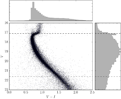
Figure 1: Color-magnitude diagram of 47 Tuc, based on data from Gilliland et al. (2000). Just as in that study, we select stars between $V=21.6$ and $17.1$ (dashed lines).

2.3 Simulated Planet Samples: $\{\mathcal{P}_{i}\}_{i\,\in\,\mathcal{S}}$ and $\mathrm{FPP}$

For most stars in $\mathcal{S}$, the corresponding Kepler star has no detected transiting planets. In such cases the star in $\mathcal{S}$ is not assigned any planets. For cases in which the Kepler star does have planets, the corresponding star in $\mathcal{S}$ is assigned planets with the same orbital period $P$ and radius $r$. By “planets” we mean KOIs with $P=0.5$-8.3 days, $r=0.5$-2 $R_{\rm Jup}$, and a DR24 disposition of either “confirmed” or “candidate”. Because the stellar radii were assigned randomly from the posterior distribution, the planetary radius $r$ is recalculated in each realization as the product of the stellar radius and the planet-to-star radius ratio listed in the KOI catalog. We neglect the uncertainty in the radius ratio because, for HJs, the leading source of uncertainty in $r$ is the uncertainty in the stellar radius.

We also need to compute the factor $(1-{\rm FPP})$ in Eqn. 2, to account for false positives. We assume FPP $=0$ for “confirmed” KOIs. For the others, we use the FPPs computed by Morton et al. (2016).

2.4 Correction for Transit Probability: $c$

The geometric transit probability is $R_{\star}/a$, which is proportional to $\rho_{\star}^{-1/3}$ at fixed orbital period. Since each star in $\mathcal{S}$ has a different mean density than the corresponding KIC star, we need to correct for the difference in transit probability. We do so by modifying the planet count around the $i$th star, $n_{{\rm det},i}$, by the factor

$$c=\left(\frac{\rho_{\star,\rm K}}{\rho_{\star,\rm 47~{}Tuc}}\right)^{1/3},$$ (5)

where $\rho_{\star,\rm K}$ and $\rho_{\star,\rm 47~{}Tuc}$ are the mean densities of the Kepler and 47 Tuc stars associated with the $i$th star, respectively.

2.5 Detection Efficiency: $d$

Gilliland et al. (2000) used inject-and-recover simulations to determine the detection efficiency of their transit search as a function of $r$, $P$, and $V$. The results are presented graphically in their Figure 4, and are reproduced in our Figure 2 along with an analytic fitting function we constructed to match the numerical results. The fitting function is of the form

$$d(r,P,V)=f(r,V)\,\frac{g(P)}{\langle g\rangle}.$$ (6)

The function $f$ is computed by linear interpolation of the data presented in the left panel of Figure 4 of Gilliland et al. (2000). In some cases we need to extrapolate $f$ beyond the ranges plotted by Gilliland et al. (2000): we assume $f=0$ for $r\leq 0.6\,R_{\rm Jup}$; $f$ achieves its maximum value at $r=1.4\,R_{\rm Jup}$; and $f(r,22)=f(r,21)$. The function

$$g(P)=0.77\exp[-0.27(P-2.95)^{0.75}]$$ (7)

is designed to match the right panel of the same figure. It matches the $P$-dependence at $V=18$ and $r=1.2\,R_{\rm Jup}$, achieves its maximum value for $P\lesssim 2.5\,\mathrm{days}$, and allows for continuous extrapolation to $P=8.3\,\mathrm{days}$. The normalization $\langle g\rangle=0.6$ represents the average over $P=2\mathchar 45\relax 6\,\mathrm{days}$, such that $f=d$ when averaging over this period range.

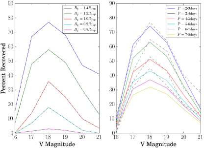
Figure 2: Dependence of planet detectability on planetary radius (left) and orbital period (right) as a function of apparent $V$ magnitude. Dashed lines are the numerical results of Gilliland et al. (2000). Solid lines are the output of our analytic fitting function (Eqn. 6). The numerical and analytic results are coincident in the left panel, by construction. In the right panel the agreement is good to within about 10%.

3 Results

We construct 1000 realizations of the star and planet samples, following the procedures described in the previous section. In each case we compute $n_{\rm det}$, the number of transiting planets that would have been detected in the HST search of 47 Tuc. The top panel of Figure 3 shows the result: the expected number of detections is $4.0^{+1.7}_{-1.4}$. Here and elsewhere the quoted value is the median of the probability distribution of $n_{\rm det}$, and the uncertainty interval covers 68.3% of the probability surrounding the median (a “one-sigma” interval).

We also constructed another 1000 realizations, this time restricting the masses of the Kepler stars to the range 0.568-0.876 $M_{\odot}$, the same range of masses as the 47 Tuc stars satisfying $17.1<V<21.6$. We perform this test because there is evidence that the planet population around low-mass stars differs from that of high-mass stars. In this case, $\mathcal{S}_{\rm K}$ consists of approximately $58,000$ stars, and the expected number of detections is $2.2^{+1.6}_{-1.1}$. This result is shown in the middle panel of Figure 3.

As a check on our procedure, we constructed an additional 1000 realizations of $\mathcal{S}$, this time assigning planets based on the same assumptions as Gilliland et al. (2000) instead of using Kepler data. Specifically, we assume that HJs exist around 0.9% of all stars, with a transit probability of $10\%$, and that all HJs have $r=1.3~{}R_{\rm Jup}$, and $P=3.5\,\mathrm{days}$. The radius and period are those of HD 209458b, the only HJ that was known at the time. In this case we find $n_{\rm det}=16.5^{+3.2}_{-3.1}$, as shown in the bottom panel of Figure 3. This agrees with the conclusions of Gilliland et al. (2000), validating our process for constructing $\mathcal{S}$ and simulating the detection efficiency.

The Kepler-based simulations give a smaller number of expected detections than 17. Table 1 breaks down the reasons for the difference. One factor is the lower occurrence rate of HJs in the Kepler field compared to the value assumed by Gilliland et al. (2000). The Kepler occurrence rate is even lower when we restrict the range of stellar masses to 0.568-0.876 $M_{\odot}$. Another important factor is that the typical value of detectability in our planet sample is only about $60\%$ of the value for the HJ assumed in Gilliland et al. (2000) (second row in Table 1). This is because the detectability is a strong function of planet radius, and the HJs in the Kepler field are often smaller than $1.3\,R_{\rm Jup}$. This situation is illustrated in Figure 4, which shows the $r$-$P$ distribution of the HJs around the Kepler stars for one realization of $\mathcal{S}_{\rm K}$.

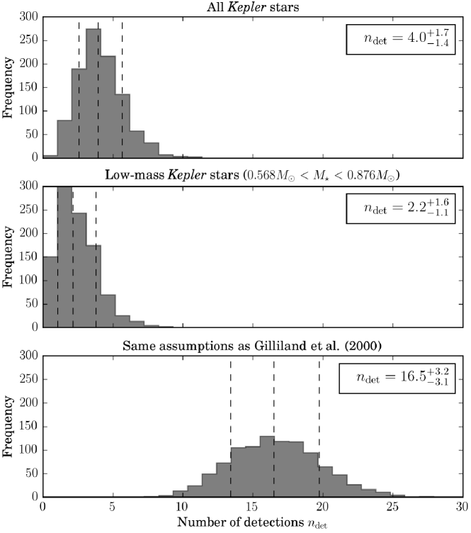
Figure 3: Distributions of the expected number of detections $n_{\rm det}$ from $1000$ simulations. From top to bottom, the results based on all the Kepler stars, mass-controlled subset of the Kepler stars, and the same assumptions as adopted in Gilliland et al. (2000) are shown. The vertical dashed lines and the numbers in the upper right boxes show $15.87\%$, $50\%$, and $84.13\%$ percentiles of the distributions.

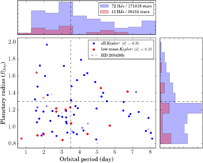
Figure 4: Planetary radius–orbital period distribution of the HJs around Kepler stars in one realization of $\mathcal{S}_{\rm K}$ taken from the simulations. Here we only show the planets larger than $0.8R_{\rm Jup}$, i.e., the ones that are essentially detectable. Blue filled circles are HJs around all the Kepler stars, while red filled diamonds show those around the low-mass subset ($0.568\,M_{\odot}<M_{\star}<0.876\,M_{\odot}$). Opacity of the points reflect the FPP values of each planet (planets with higher FPPs are more transparent). Vertical and horizontal dashed lines indicate the values of HD 209458b ($P=3.5\,\mathrm{days}$ and $r=1.3\,R_{\rm Jup}$), which are assumed by Gilliland et al. (2000). The inset in the top panel shows the sum of $1-\mathrm{FPP}$ for all the plotted HJs and the number of KIC stars in this $\mathcal{S}_{\rm K}$. The inset in the middle panel shows detection efficiency $d$ averaged over all the HJs in the plot with the weight $1-\mathrm{FPP}$.

Table 1: Typical Values of Each Factor in Equations (1) and (2) from our Simulations

	Gilliland et al. (2000)	All Kepler	Low-mass Kepler	RV Sample
Transiting HJ Occurrence $\sum_{\mathcal{P}}(1-\mathrm{FPP})/34,091$	$(8\mathchar 45\relax 10)\times 10^{-4}$	$3.9\times 10^{-4}$	$1.8\times 10^{-4}$	$14\times 10^{-4}$
Average Detectability $\langle d\rangle$	$0.54$	$0.34$	$0.31$	$0.38$
Average Transit-Probability Correction $\langle c\rangle$	$\cdots$	$0.84$	$1.1$	$0.79$
Yield from $34,091$ Stars	$17$	$4.0$	$2.2$	$15$

Note. — In columns 2 and 3, the values of transiting HJ occurrence represent $1-\mathrm{FPP}$ summed over practically detectable HJs in $\mathcal{P}$ ($P=0.5$-$8.3$ days, $r=0.8$-2 $R_{\rm Jup}$), divided by $34,091$. The values for detectability and the transit-probability correction are the averages for all the HJs in this range, weighted by $1-\mathrm{FPP}$. The quoted values are the medians based on 1000 simulations. Note that the last row is approximately the product of the first three rows and $34,091$.

4 Discussion

4.1 Occurrence Rate of Kepler Hot Jupiters

One of the critical factors that reduce the number of expected detections is the lower occurrence rate of transiting HJs in the Kepler sample, compared to the rate assumed by Gilliland et al. (2000). Howard et al. (2012) also measured the HJ occurrence rate based on Kepler data. To facilitate a comparison between their study and ours, we calculate the occurrence rate of HJs, as opposed to transiting HJs. To do so we perform another set of simulations, this time with $\mathcal{S}=\mathcal{\tilde{S}}_{\rm K}$, and replacing Eqn. 2 with

$$n_{{\rm det},i}=\sum_{j\,\in\,\mathcal{P}_{i}}(1-{\rm FPP}_{j})\frac{a_{j}}{R_{\star,i}},$$ (8)

i.e., we divide by the transit probability $R_{\star}/a$. We adopt the value of $a/R_{\star}$ from the KOI catalog, assuming a circular orbit and neglecting the uncertainty. For consistency with Howard et al. (2012) we also modify the definition of “planets” in Section 2.3 to be those with $P<10\,\mathrm{days}$ and $r=0.8$-2 $R_{\rm Jup}$. Through this procedure we find $f_{\rm HJ}=0.43^{+0.07}_{-0.06}\%$, in agreement with the value of 0.4% found by Howard et al. (2012).

When restricting the Kepler stars to the same range of masses as the stars that were searched in 47 Tuc, we find $f_{\rm HJ}=0.24^{+0.10}_{-0.09}\%$, which is smaller than the rate obtained for the entire sample of stars. This suggests that the low-mass Kepler stars have an even lower HJ occurrence rate. The statistical significance of the difference is modest, because of the relatively small number of HJs ($\approx$10) in the restricted sample. This possible dependence of HJ occurrence on stellar mass will come into sharper focus after the TESS mission (Ricker et al., 2014), which should provide a larger sample of transiting HJs around a wide range of stellar types.

4.2 Comparison with RV Samples

Wright et al. (2012) measured the HJ occurrence rate using the Doppler or radial-velocity (RV) technique. Based on a sample of 10 HJs found within a set of 836 stars, they found $f_{\rm HJ}=10/836=(1.2\pm 0.4)\%$, which is higher than our result by 1.9$\sigma$. If the occurrence rate is really 1.2%, the number of expected detections in the 47 Tuc survey would be much higher than the results presented in the previous section. To demonstrate this, we perform another round of simulations using the RV sample from Wright et al. (2012) instead of Kepler stars; this time $\mathcal{S}_{\rm K}$ consists of $836$ stars considered in the RV sample of Wright et al. (2012), among which $10$ are associated with HJs listed in Table 2. One obstacle is that most of the HJs in the RV sample do not transit, and their radii are unknown; even their true masses are unknown. We must nevertheless assign them radii in our simulations. We do so by assigning each planet a random orbital orientation (uniform in $\cos I$) and calculating the planet mass $m$ based on the measured value of $m\sin I$. Then we calculate $r$ using the relations between planetary mass, radius, and incident flux $F$ presented by Weiss et al. (2013). We also add Gaussian random deviates to $r$ to account for the scatter in the $m/r/F$ relation ($1.15\,R_{\oplus}$ for $m>150\,M_{\oplus}$ and $1.41\,R_{\oplus}$ for smaller $m$). The result for the number of expected detections in the 47 Tuc survey is $15.2^{+7.1}_{-5.9}$. This is larger than our Kepler-based results and compatible with the original estimate of Gilliland et al. (2000). The difference is mainly due to the higher $f_{\rm HJ}$ of the RV sample, with a smaller contribution from somewhat higher detectability (larger planets).

The RV-based result has a higher statistical uncertainty than our Kepler-based result. There are a few additional reasons to attach greater weight to the Kepler-based result. The RV sample was constructed post facto from stars originally selected for undocumented reasons. Mayor et al. (2011) performed an independent RV-based analysis of similar stars, finding 5 HJs within a sample of 822 stars (see their Sec. 4.2), and giving $f_{\rm HJ}=0.6_{-0.2}^{+0.3}\%$. This is half the value reported by Wright et al. (2012), and within 1$\sigma$ of the Kepler-based result. Table 1 of Mayor et al. (2011) reports a higher rate of 0.89%, but this includes planets with masses as low as 0.16 $M_{\rm Jup}$ and periods $<$11 days rather than 10 days. We do not know why the seemingly more arbitrary upper limit of 11 days was chosen, illustrating the difficulty of analyzing post facto samples. Furthermore, our method is more direct by associating real planets and their properties to 47 Tuc stars, rather than inferring an occurrence rate for a certain sharply-defined category of planets from one survey, and then using that rate to interpret the results from a different survey.

A separate issue is that the RV surveys do not provide much information about the range of stellar masses (0.568-0.876 $M_{\odot}$) spanned by the 47 Tuc stars. The RV sample of Wright et al. (2012) includes only one HJ in that mass range, causing a large Poisson uncertainty in the occurrence rate.

Table 2: Properties of HJs and their Host Stars in the RV Sample of Wright et al. (2012)

Name	$m\sin I$ ($M_{\rm Jup}$)	$P$ (day)	$M_{\star}$ ($M_{\odot}$)	$R_{\star}$ ($R_{\odot}$)	$T_{\rm eff}$ (K)	[Fe/H]	Reference
$\upsilon$ And (HD 9826) b	$0.669\pm 0.026$	$4.6$	$1.31\pm 0.03$	$1.573\pm 0.019$	$6213$	$0.15$	1
$\tau$ Boo (HD 120136) b	$4.12\pm 0.15$	$3.3$	$1.35\pm 0.03$	$1.419\pm 0.019$	$6387$	$0.23$	1
$51$ Peg (HD 217014) b	$0.461\pm 0.016$	$4.2$	$1.10\pm 0.03$	$1.138\pm 0.016$	$5787$	$0.20$	1
HD 217107 b	$1.401\pm 0.048$	$7.1$	$1.108\pm 0.043$	$1.500\pm 0.030$	$5704$	$0.389\pm 0.030$	2
HD 185269 b	$0.954\pm 0.069$	$6.8$	$1.28\pm 0.1$	$1.88\pm 0.1$	$5980$	$0.11\pm 0.05$	3
HD 209458 b	$0.689\pm 0.024$	$3.5$	$1.18\pm 0.06$	$1.203\pm 0.061$	$6092$	$0.00\pm 0.05$	1,4,7
HD 189733 b	$1.140\pm 0.056$	$2.2$	$0.846^{+0.068}_{-0.049}$	$0.805\pm 0.016$	$4875$	$-0.03\pm 0.08$	4,5,7
HD 187123 b	$0.510\pm 0.017$	$3.1$	$1.037\pm 0.025$	$1.143\pm 0.039$	$5815$	$0.121\pm 0.030$	2
HD 46375 b	$0.2272\pm 0.0091$	$3.0$	$0.93\pm 0.03$	$1.003\pm 0.039$	$5285$	$0.24$	1
HD 149143 b	$1.328\pm 0.078$	$4.0$	$1.21\pm 0.1$	$1.49\pm 0.1$	$5884$	$0.26\pm 0.05$	6

4.3 Other Globular Cluster Surveys

We have focused on the survey by Gilliland et al. (2000) because it is the most sensitive survey that has yet been conducted for planets in globular clusters. Weldrake et al. (2005) used ground-based observations to perform a search for transiting planets in a sample of $21,920$ stars in a less crowded region of 47 Tuc. They expected to find 7 planets if the planet population were identical to that of field stars, and found none. However, although they took into account the period-dependence of the selection function, they do not appear to have taken into account the much stronger dependence on planet radius. Moreover, their expectation was based on a HJ occurrence rate of 0.8%, larger than the Kepler value. Using the methodology presented in this paper, we expect that the number of expected detections would also be reduced by about a factor of 4, as was the case with the HST survey. This would cause the apparent difference with field stars to be statistically insignificant. The same argument would apply to the ground-based survey of $\omega$ Centauri by Weldrake et al. (2008), which was only sensitive to relatively large HJs ($\gtrsim$1.5 $R_{\rm Jup}$).

Nascimbeni et al. (2012) conducted an HST search for transiting planets among $5,078$ members of NGC 6397. They were sensitive to giant planets with periods between $0.2$-$14$ days, and did not detect any planets. They performed a statistical analysis of a subsample of $2,215$ M-dwarfs and could not rule out the hypothesis that the cluster stars have the same planet population as field stars. This is not surprising, given the relatively small number of stars in the sample.

4.4 Metallicity Effect

We controlled for stellar mass by restricting the Kepler comparison sample to the same range of masses as the stars that were searched in 47 Tuc. In addition to mass, the stellar metallicity is thought to be strongly linked to the HJ occurrence rate (see, e.g., Johnson et al., 2010). It has long been known that a low stellar metallicity is associated with a low occurrence rate of giant planets with orbital distances $\lesssim$1 AU. However, with the available data it is impossible to control for metallicity. The stars in 47 Tuc have $\mathrm{[Fe/H]}\approx-0.7$, while Kepler stars have a mean [Fe/H] $\approx 0$ (Dong et al., 2014; Guo et al., 2016). We cannot restrict the Kepler sample to low-metallicity stars because reliable metallicities are only available for a small number of stars, and most likely the Kepler field does not include enough low-metallicity stars for our resampling procedure to be effective.

Instead, we simply note that the number of expected detections has been lowered to such a degree that we are unable to say confidently whether the lack of detected planets could be attributable to the low metallicity of 47 Tuc. After controlling for stellar mass (but not metallicity), the number of expected detections is $2.2^{+1.6}_{-1.1}$, only marginally inconsistent with zero. Controlling for metallicity would lower the number of expected detections still further. For example, Johnson et al. (2010) found that giant-planet occurrence scales as $10^{1.2\mathrm{[Fe/H]}}$; if we assume this is also true of stars in globular clusters, then the mean number of expected detections becomes less than unity for $\mathrm{[Fe/H]}\approx-0.29$. Schlaufman (2014) argued for an even stronger dependence on metallicity, with giant-planet occurrence scaling as $10^{2.3\mathrm{[Fe/H]}}$. Using that relation, the mean number of expected detections becomes less than unity for $\mathrm{[Fe/H]}\approx-0.15$.

4.5 Choice of Stellar Models

We adopted stellar parameters for the 47 Tuc stars based on the stellar-evolutionary models of Bergbusch & Vandenberg (1992), following Gilliland et al. (2000). More recent stellar-evolutionary models are available. Adopting a different set of stellar models alters the stellar mass and radius for a given $V$ magnitude. This affects the correction for transit probability (Section 2.4), and the detectability as a function of $V$, $r$, and $P$, by altering the transit depth and duration.

To check on the sensitivity of our results to the choice of stellar-evolutionary models, we recompute the relation between $(M_{\star},R_{\star})$ and $V$-magnitude using the Dartmouth isochrones (Dotter et al., 2008). We assume a cluster age of $11.6\,\mathrm{Gyr}$, $\mathrm{[Fe/H]}=-0.69$, $\mathrm{[\alpha/H]}=0.20$, and helium mass fraction of $0.2525$. These values are nearly the same as those obtained by Correnti et al. (2016) via isochrone fitting to an HST infrared color-magnitude diagram, but are slightly modified to match the color-magnitude diagram in Figure 1 with the distance modulus $13.4$ and $E(V-I)=0.05$.

Using this model, we recompute $\rho_{\star}^{-1/3}$ (relevant to the transit probability correction) and $\sqrt{\rho_{\star}^{-1/3}R_{\star}^{-2}}$ (relevant to detectability) for each of the stars in 47 Tuc and compare them to those computed with the models of Bergbusch & Vandenberg (1992). We find that the differences are only a few percent, on average, and no larger than $25\%$ for any choice of $V$. We conclude that the choice of stellar-evolutionary models does not significantly affect our results.

4.6 Effect of Extrapolating Detection Efficiency

To cover the full range of periods and sizes of Kepler HJs, we needed to extrapolate the numerical results for detection efficiency beyond the limits presented in Figure 4 of Gilliland et al. (2000). Specifically we assumed

• $f=0$ for $r\leq 0.6\,R_{\rm Jup}$. This seems a safe assumption because $f$ is already very close to zero at $r=0.8\,R_{\rm Jup}$.

• $g$ saturates at its maximum value for $P\lesssim 2.5\,\mathrm{days}$. This too seems a safe assumption, and (given our functional form) is necessary to maintain $d\leq 1$ at short periods.

• $f$ saturates at its maximum value for $r\geq 1.4\,R_{\rm Jup}$, regardless of $V$.

• $g$ between $P=6$-8.3 days is given by smooth extrapolation from $P<6$ days.

The validity of the last two assumptions is not so obvious. It is conceivable that $f$ could increase beyond $r=1.4\,R_{\rm Jup}$; this would not violate $d\leq 1$ as long as $V\neq 18$. It is also conceivable that $g$ drops abruptly as $P$ approaches the total duration (8.3 days) of the time series that was searched.

To check on the sensitivity of our results to these two assumptions, we perform additional rounds of simulations using extreme forms of $d$:

1. $f=f_{\rm max}$ for $r\geq 1.6\,R_{\rm Jup}$, regardless of $V$. Here $f_{\rm max}$ is the maximum possible value satisfying $d\leq 1$, and is equal to $f(1.4\,R_{\rm Jup},18)$.

2. $g(P)=0$ for $P\geq 6\,\mathrm{days}$.

In the first case we find $n_{\rm det}=4.1^{+1.8}_{-1.4}$ for the full Kepler sample, and $n_{\rm det}=2.3^{+1.7}_{-1.2}$ for the low-mass Kepler sample. In the second case, we find $n_{\rm det}=3.7^{+1.7}_{-1.3}$ and $n_{\rm det}=2.0^{+1.5}_{-1.2}$ for the full and low-mass samples, respectively. These results show that our conclusions are fairly insensitive to the manner in which we have extrapolated the detection efficiency.

5 Summary and conclusion

Among the many gifts of the Kepler mission is a very large sample of stars that have been exhaustively searched for the types of transiting planets that could have been detected in the prior HST survey of 47 Tuc by Gilliland et al. (2000). The Kepler survey thereby provides the best and most reliable means to try and interpret the null result of the 47 Tuc survey. We have used a resampling technique to test the hypothesis that the Kepler stars and the 47 Tuc stars have the same planet population; specifically, the same occurrence rate and radius/period distribution for giant planets. Under this hypothesis, we found that the number of transiting planets that should have been detected in the 47 Tuc survey is $4.0^{+1.7}_{-1.4}$. Thus, the hypothesis can only be rejected at the $\approx$3$\sigma$ level. We also tested the hypothesis that the 47 Tuc stars and the Kepler stars over the same range of mass have the same population of close-in giant planets. In this case we find that only $2.2^{+1.6}_{-1.1}$ planets should have been detected in the 47 Tuc survey, and there is a $\approx$15% chance that no planets would be found. Both of these results lead to a lower degree of confidence that the planet populations are different than was originally thought.

The null result reported by Gilliland et al. (2000) remains the best constraint on the planet occurrence in globular clusters ever obtained, and suggests that close-in giant planets are rarer in 47 Tuc than in the field, but with a low statistical significance. We are therefore still far from understanding the planet population within globular clusters, and what might cause it to differ from that of other types of stars. A more sensitive search for planets in globular clusters is needed.

References

- Adams et al. (2004) Adams, F. C., Hollenbach, D., Laughlin, G., & Gorti, U. 2004, ApJ, 611, 360
- Armitage (2000) Armitage, P. J. 2000, A&A, 362, 968
- Backer et al. (1993) Backer, D. C., Foster, R. S., & Sallmen, S. 1993, Nature, 365, 817
- Batygin et al. (2016) Batygin, K., Bodenheimer, P. H., & Laughlin, G. P. 2016, ApJ, 829, 114
- Bergbusch & Vandenberg (1992) Bergbusch, P. A., & Vandenberg, D. A. 1992, ApJS, 81, 163
- Bonnell et al. (2001) Bonnell, I. A., Smith, K. W., Davies, M. B., & Horne, K. 2001, MNRAS, 322, 859
- Borucki et al. (2010) Borucki, W. J., Koch, D., Basri, G., et al. 2010, Science, 327, 977
- Boyajian et al. (2015) Boyajian, T., von Braun, K., Feiden, G. A., et al. 2015, MNRAS, 447, 846
- Burke et al. (2015) Burke, C. J., Christiansen, J. L., Mullally, F., et al. 2015, ApJ, 809, 8
- Charbonneau et al. (2000) Charbonneau, D., Brown, T. M., Latham, D. W., & Mayor, M. 2000, ApJ, 529, L45
- Correnti et al. (2016) Correnti, M., Gennaro, M., Kalirai, J. S., Brown, T. M., & Calamida, A. 2016, ApJ, 823, 18
- Davies & Sigurdsson (2001) Davies, M. B., & Sigurdsson, S. 2001, MNRAS, 324, 612
- de Kok et al. (2013) de Kok, R. J., Brogi, M., Snellen, I. A. G., et al. 2013, A&A, 554, A82
- Debes & Jackson (2010) Debes, J. H., & Jackson, B. 2010, ApJ, 723, 1703
- Dong et al. (2014) Dong, S., Zheng, Z., Zhu, Z., et al. 2014, ApJ, 789, L3
- Dotter et al. (2008) Dotter, A., Chaboyer, B., Jevremović, D., et al. 2008, ApJS, 178, 89
- Feng et al. (2015) Feng, Y. K., Wright, J. T., Nelson, B., et al. 2015, ApJ, 800, 22
- Fischer & Valenti (2005) Fischer, D. A., & Valenti, J. 2005, ApJ, 622, 1102
- Fischer et al. (2006) Fischer, D. A., Laughlin, G., Marcy, G. W., et al. 2006, ApJ, 637, 1094
- Fregeau et al. (2006) Fregeau, J. M., Chatterjee, S., & Rasio, F. A. 2006, ApJ, 640, 1086
- Gilliland et al. (2000) Gilliland, R. L., Brown, T. M., Guhathakurta, P., et al. 2000, ApJ, 545, L47
- Gu et al. (2003) Gu, P.-G., Lin, D. N. C., & Bodenheimer, P. H. 2003, ApJ, 588, 509
- Guo et al. (2016) Guo, X., Johnson, J. A., Mann, A. W., et al. 2016, ArXiv e-prints, arXiv:1612.01616
- Henry et al. (2000) Henry, G. W., Marcy, G. W., Butler, R. P., & Vogt, S. S. 2000, ApJ, 529, L41
- Howard et al. (2012) Howard, A. W., Marcy, G. W., Bryson, S. T., et al. 2012, ApJS, 201, 15
- Johnson et al. (2010) Johnson, J. A., Aller, K. M., Howard, A. W., & Crepp, J. R. 2010, PASP, 122, 905
- Johnson et al. (2006) Johnson, J. A., Marcy, G. W., Fischer, D. A., et al. 2006, ApJ, 652, 1724
- Mathur et al. (2016) Mathur, S., Huber, D., Batalha, N. M., et al. 2016, ArXiv e-prints, arXiv:1609.04128
- Mayor et al. (2011) Mayor, M., Marmier, M., Lovis, C., et al. 2011, arXiv:1109.2497
- McWilliam & Bernstein (2008) McWilliam, A., & Bernstein, R. A. 2008, ApJ, 684, 326
- Morton et al. (2016) Morton, T. D., Bryson, S. T., Coughlin, J. L., et al. 2016, ApJ, 822, 86
- Nascimbeni et al. (2012) Nascimbeni, V., Bedin, L. R., Piotto, G., De Marchi, F., & Rich, R. M. 2012, A&A, 541, A144
- Ricker et al. (2014) Ricker, G. R., Winn, J. N., Vanderspek, R., et al. 2014, in Proc. SPIE, Vol. 9143, Space Telescopes and Instrumentation 2014: Optical, Infrared, and Millimeter Wave, 914320
- Santos et al. (2001) Santos, N. C., Israelian, G., & Mayor, M. 2001, A&A, 373, 1019
- Schlaufman (2014) Schlaufman, K. C. 2014, ApJ, 790, 91
- Sigurdsson (1992) Sigurdsson, S. 1992, ApJ, 399, L95
- Spurzem et al. (2009) Spurzem, R., Giersz, M., Heggie, D. C., & Lin, D. N. C. 2009, ApJ, 697, 458
- Thompson (2013) Thompson, T. A. 2013, MNRAS, 431, 63
- Torres et al. (2008) Torres, G., Winn, J. N., & Holman, M. J. 2008, ApJ, 677, 1324
- Valenti & Fischer (2005) Valenti, J. A., & Fischer, D. A. 2005, ApJS, 159, 141
- Weiss et al. (2013) Weiss, L. M., Marcy, G. W., Rowe, J. F., et al. 2013, ApJ, 768, 14
- Weldrake et al. (2008) Weldrake, D. T. F., Sackett, P. D., & Bridges, T. J. 2008, ApJ, 674, 1117
- Weldrake et al. (2005) Weldrake, D. T. F., Sackett, P. D., Bridges, T. J., & Freeman, K. C. 2005, ApJ, 620, 1043
- Winn (2010) Winn, J. N., “Exoplanet Transits and Occultations,” in Exoplanets, ed. S. Seager, University of Arizona Press (Tucson, AZ, 2010), p. 55-77
- Wright et al. (2012) Wright, J. T., Marcy, G. W., Howard, A. W., et al. 2012, ApJ, 753, 160