Inference via low-dimensional couplings

Abstract

We investigate the low-dimensional structure of deterministic transformations between random variables, i.e., transport maps between probability measures. In the context of statistics and machine learning, these transformations can be used to couple a tractable “reference” measure (e.g., a standard Gaussian) with a target measure of interest. Direct simulation from the desired measure can then be achieved by pushing forward reference samples through the map. Yet characterizing such a map—e.g., representing and evaluating it—grows challenging in high dimensions. The central contribution of this paper is to establish a link between the Markov properties of the target measure and the existence of low-dimensional couplings, induced by transport maps that are sparse and/or decomposable. Our analysis not only facilitates the construction of transformations in high-dimensional settings, but also suggests new inference methodologies for continuous non-Gaussian graphical models. For instance, in the context of nonlinear state-space models, we describe new variational algorithms for filtering, smoothing, and sequential parameter inference. These algorithms can be understood as the natural generalization—to the non-Gaussian case—of the square-root Rauch–Tung–Striebel Gaussian smoother.

Keywords: transport map, variational inference, graphical model, sparsity, joint parameter and state estimation

1 Introduction

This paper studies the low-dimensional structure of transformations between random variables. Such transformations, which can be understood as transport maps between probability measures [117], are ubiquitous in statistics and machine learning: they can be used for posterior sampling [80], possibly via deep neural networks [95]; for accelerating Markov chain Monte Carlo or importance sampling algorithms [83, 48]; or as the building blocks of implicit generative models [58, 44, 77] and flexible methods for density estimation [115, 30].

In the context of variational inference [9], a transport map can be used to define a deterministic coupling between a tractable reference measure $\bm{\nu}_{\eta}$ that we can easily simulate (e.g., a standard Gaussian) and an arbitrary target measure $\bm{\nu}_{\pi}$ that we wish to characterize (e.g., a posterior distribution). Given i.i.d. samples $(\bm{X}_{i})$ from the reference measure, we can evaluate the transport map to obtain i.i.d. samples $(T(\bm{X}_{i}))$ from the target. In other words, the map allows any expectation $\int g\,\rm{d}\bm{\nu}_{\pi}$ over the target measure to be rewritten as an integral over the reference measure,

$$\int g(\bm{x})\,{\rm d}\bm{\nu}_{\pi}(\bm{x})=\int g(T(\bm{x}))\,{\rm d}\bm{\nu}_{\eta}(\bm{x})\,,$$

thus enabling the use of standard integration techniques for the tractable $\bm{\nu}_{\eta}$, including Monte Carlo sampling and deterministic quadrature [76, 118, 80, 29].

We focus on absolutely continuous measures $(\bm{\nu}_{\eta},\bm{\nu}_{\pi})$ on $\mathbb{R}^{n}$, for which the existence of a transport map $T:\mathbb{R}^{n}\rightarrow\mathbb{R}^{n}$ is guaranteed [103]. Such a map, however, is seldom unique. Identifying a particular map requires imposing additional structure on the problem. Optimal transport maps, for instance, define couplings that minimize a particular integrated transport cost expressing the effort required to rearrange samples [117]. The analysis of such maps underpins a vast field that links geometry and partial differential equations, with applications in fluid dynamics, economics, statistics [32, 56], and beyond. In recent years, several other couplings have been proposed for use in statistical problems, e.g., parametric approximations [80] of the Knothe–Rosenblatt rearrangement [97, 61], couplings induced by the flows of ODEs [49, 1, 22], and couplings induced by the composition of many simple maps, including deep neural networks [69, 115, 95]. Yet the construction, representation, and evaluation of all these maps grows challenging in high dimensions. In the setting considered here, a transport map is a function from $\mathbb{R}^{n}$ onto itself; without specifying further structure, representing such a map or even realizing its action is often intractable as $n$ increases.

The central contribution of this paper is to establish a link between the conditional independence structure of the reference-target pair—the so-called Markov properties [65] of $\bm{\nu}_{\eta}$ and $\bm{\nu}_{\pi}$—and the existence of low-dimensional couplings. These couplings are induced by transport maps that are sparse and/or decomposable. A sparse map consists of scalar-valued component functions that each depend only on a few input variables, whereas a decomposable map factorizes as the exact composition of finitely many functions of low effective dimension (i.e., $T=T_{1}\circ\cdots\circ T_{\ell}$, where each $T_{i}$ differs from the identity map only along a subset of its components). These properties, and their combinations, dramatically reduce the complexity of representing a transport map and can be deduced before the map is explicitly computed.

The utility of these results is twofold. First, they make the construction of couplings—and hence the characterization of complex probability distributions—tractable for a large class of inference problems. In particular, these results can be exploited in state-of-the-art approaches for the numerical computation of transport maps, including normalizing flows [95] or Stein variational algorithms [1, 69, 27]. Second, these results suggest new algorithmic approaches for important classes of statistical models. For instance, our analysis of sparse triangular maps provides a general framework for describing continuous and non-Gaussian Markov random fields, and for exploiting the conditional independence structure of these fields in computation. Our analysis of decomposable transport maps yields new variational algorithms for sequential inference in nonlinear and non-Gaussian state space models. These algorithms characterize the full Bayesian solution to the smoothing and joint state–parameter inference problems by means of a decomposable transport map, which is constructed (recursively) in a single forward pass using local operations. These algorithms can be understood as the natural generalization, to the non-Gaussian case, of the square-root Rauch-Tung-Striebel Gaussian smoother. Moreover, the results presented in this paper underpin recent efforts in structure learning for non-Gaussian graphical models [78], and novel approaches to the filtering of high-dimensional spatiotemporal processes [109, Chapter 6]. Overall, we propose a range of techniques to address problems of inference in continuous non-Gaussian graphical models.

The paper is organized as follows. Section 2 introduces some notation used throughout the paper. Section 3 reviews the Knothe-Rosenblatt rearrangement, a key coupling for our analysis, while Section 4 briefly recalls some standard terminology for Markov random fields and graphical models. The main results are in Sections 5–7: Section 5 addresses the sparsity of triangular transports, while Section 6 introduces and develops the concept of decomposable transport maps for general Markov networks. These two sections can be read independently. Section 7 specializes the theory of Section 6 to state-space models, introducing new variational algorithms for filtering, smoothing, and parameter inference. Section 8 illustrates aspects of the theory with numerical examples. A final discussion is presented in Section 9. Appendix A collects some technical details on the Knothe-Rosenblatt rearrangement and its generalizations. Appendix B contains the proofs of the main results. Appendix C provides pseudocode for our variational algorithms applied to state-space models, and additional numerical experiments are described in Appendix D. Code and all numerical examples are available online.

2 Notation

Here, we collect some useful notation used throughout the paper.

Notation for functions, sets, and graphs

For a pair of functions $f$ and $g$, we denote their composition by $f\circ g$. We denote by $\partial_{k}f$ the partial derivative of $f$ with respect to its $k$th input variable. By $\partial_{k}f=0$, we mean that the function $f$ does not depend on its $k$th input variable. Depending on the context, we can identify a matrix $Q$ with its corresponding linear map, given by $\bm{x}\mapsto Q\bm{x}$.

For all $n>0$, we let $\mathbb{N}_{n}=\{1,\ldots,n\}$ denote the set of the first $n$ integers. For any pair of sets, $\mathcal{A}\subset\mathcal{B}$ means that $\mathcal{A}$ is a subset of $\mathcal{B}$ (including the possibility of $\mathcal{A}=\mathcal{B}$). We denote by $|\mathcal{A}|$ the cardinality of $\mathcal{A}$.

Given a graph $\bm{\mathcal{G}}=(\mathcal{V},\mathcal{E})$ with vertices $\mathcal{V}$ and edges $\mathcal{E}$, we denote by ${\rm Nb}(k,\bm{\mathcal{G}})$ the neighborhood of a node $k$ in $\bm{\mathcal{G}}$, while for any set $\mathcal{A}\subset\mathcal{V}$, we denote by $\bm{\mathcal{G}}_{\mathcal{A}}=(\mathcal{V}^{\prime},\mathcal{E}^{\prime})$ the subgraph given by $\mathcal{V}^{\prime}=\mathcal{A}$ and $\mathcal{E}^{\prime}=\mathcal{E}\cap(\mathcal{A}\times\mathcal{A})$.

Notation for measures and densities

In this paper, we mostly consider probability measures on $\mathbb{R}^{n}$ that are absolutely continuous with respect to the Lebesgue measure, $\bm{\lambda}$, and that are fully supported. We denote the set of such measures by $\mathscr{M}_{+}(\mathbb{R}^{n})$. The density of a measure will always be intended with respect to $\bm{\lambda}$. For a pair of measures $\bm{\nu}_{1},\bm{\nu}_{2}$, $\bm{\nu}_{1}\ll\bm{\nu}_{2}$ means that $\bm{\nu}_{1}$ is absolutely continuous with respect to $\bm{\nu}_{2}$.

For any measure $\bm{\nu}$ and measurable map $T$, we denote by $T_{\sharp}\bm{\nu}$ the pushforward measure given by $\bm{\nu}\circ T^{-1}$, where for any set $\mathcal{B}$, $T^{-1}(\mathcal{B})$ is the set-valued preimage of $\mathcal{B}$ under $T$. Similarly, we denote by $T^{\sharp}\bm{\nu}$ the pullback measure given by $\bm{\nu}\circ T$. Given a measure $\bm{\nu}$ with density $\pi$ and a map $T$, we denote by $T_{\sharp}\pi$ the density of $T_{\sharp}\bm{\nu}$, provided it exists (depending on $T$). We call $T_{\sharp}\pi$ the pushforward density of $\pi$ by $T$. Similarly, we define the pullback density $T^{\sharp}\pi$ as the density of $T^{\sharp}\bm{\nu}$, provided it exists. Whether the map $T$ preserves the absolute continuity of the measure depends on the regularity of $T$. For instance, if $T:\mathbb{R}^{n}\rightarrow\mathbb{R}^{n}$ is a diffeomorphism—i.e., a differentiable bijection with differentiable inverse—then one has:

$$T_{\sharp}\pi(\bm{x})=\pi(T^{-1}(\bm{x}))\,|\det\nabla T^{-1}(\bm{x})|,\qquad T^{\sharp}\pi(\bm{x})=\pi(T(\bm{x}))\,|\det\nabla T(\bm{x})|,$$ (2.1)

where $\nabla T(\bm{x})$ denotes the Jacobian of $T$ at $\bm{x}$. The regularity assumptions on $T$ can be substantially weakened as long as one modifies (2.1) appropriately [98, 112, 38]. We will give one such example shortly when dealing with triangular maps (see Section 3 or Appendix A). We denote by $\int f(\bm{x})\,\bm{\nu}({\rm d}\bm{x})$ the integration of a measurable function $f:\mathbb{R}^{n}\rightarrow\mathbb{R}$ with respect to a measure $\bm{\nu}$. For the Lebesgue measure, we simplify our notation as $\int f(\bm{x})\,\bm{\lambda}({\rm d}\bm{x})=\int f(\bm{x})\,{\rm d}\bm{x}$. Given a pair $\eta,\pi$ of probability densities and a map $T:\mathbb{R}^{n}\rightarrow\mathbb{R}^{n}$, we say that $T$ pushes forward $\eta$ to $\pi$ if and only if $T$ couples the corresponding probability measures, i.e., $T_{\sharp}\bm{\nu}_{\eta}=\bm{\nu}_{\pi}$, with $\bm{\nu}_{\eta}(\mathcal{B})=\int_{\mathcal{B}}\eta(\bm{x})\,{\rm d}\bm{x}$ and $\bm{\nu}_{\pi}(\mathcal{B})=\int_{\mathcal{B}}\pi(\bm{x})\,{\rm d}\bm{x}$ for all measurable sets $\mathcal{B}$. (Notice that $T_{\sharp}\eta$ need not be given by (2.1) since we are not specifying any regularity on $T$.)

When it is clear from context, we will freely omit the qualifier a.e. to indicate a property that holds up to a set of measure zero.

Notation for random variables

We use boldface capital letters, e.g., $\bm{X}$, to denote random variables on $\mathbb{R}^{n}$ with $n>1$, while we write scalar-valued random variables as $X$. The law of a random variable $\bm{X}$ defined on a probability space $(\Omega,\mathbb{P})$ is given by $\bm{X}_{\sharp}\mathbb{P}$. For a measure $\bm{\nu}$, $\bm{X}\sim\bm{\nu}$ means that $\bm{X}$ has law $\bm{\nu}$. If $\bm{X}=(\bm{X}_{1},\ldots,\bm{X}_{p})$ is a collection of random variables and $\mathcal{A}\subset\mathbb{N}_{p}$, then $\bm{X}_{\mathcal{A}}=(\bm{X}_{i},i\in\mathcal{A})$ denotes a subcollection of $\bm{X}$. In the same way, for $j<k$, $\bm{X}_{j:k}=(\bm{X}_{j},\bm{X}_{j+1},\ldots,\bm{X}_{k})$. If $\bm{X}=(\bm{X}_{1},\ldots,\bm{X}_{p})$ has joint density $\pi$ and $\mathcal{A}\subset\mathbb{N}_{p}$, we denote by $\pi_{\bm{X}_{\mathcal{A}}}$ the marginal of $\pi$ along $\bm{X}_{\mathcal{A}}$, i.e., $\pi_{\bm{X}_{\mathcal{A}}}(\bm{x}_{\mathcal{A}})=\int\pi(\bm{x})\,{\rm d}\bm{x}_{\mathbb{N}_{p}\setminus\mathcal{A}}$. If $\pi$ is the density of $\bm{Z}=(\bm{X},\bm{Y})$, we denote by $\pi_{\bm{X}|\bm{Y}}$ the density of $\bm{X}$ given $\bm{Y}$, where

$$\pi_{\bm{X}|\bm{Y}}(\bm{x}|\bm{y})=\begin{cases}\pi_{\bm{X},\bm{Y}}(\bm{x},\bm{y})/\pi_{\bm{Y}}(\bm{y})&\mbox{if }\pi_{\bm{Y}}(\bm{y})\neq 0\\ 0&\mbox{otherwise}.\end{cases}$$ (2.2)

We denote independence of a pair of random variables $\bm{X},\bm{Y}$ by $\bm{X}\perp\!\!\!\perp\bm{Y}$. In the same way, $\bm{X}\perp\!\!\!\perp\bm{Y}|\bm{R}$ means that $\bm{X}$ and $\bm{Y}$ are independent given a third random variable $\bm{R}$.

3 Triangular transport maps: a building block

An important transport for our analysis is the Knothe-Rosenblatt (KR) rearrangement on $\mathbb{R}^{n}$ [97, 61, 10]. For a pair of measures $\bm{\nu}_{\eta},\bm{\nu}_{\pi}\in\mathscr{M}_{+}(\mathbb{R}^{n})$, with densities $\eta$ and $\pi$, respectively, the KR rearrangement is the unique monotone increasing lower triangular measurable map that pushes forward $\bm{\nu}_{\eta}$ to $\bm{\nu}_{\pi}$, i.e., $T_{\sharp}\bm{\nu}_{\eta}=\bm{\nu}_{\pi}$ [13, 10]. Here, monotonicity is with respect to the lexicographic order on $\mathbb{R}^{n}$, while uniqueness is up to $\bm{\nu}_{\eta}$-null sets [10]. A lower triangular map $T:\mathbb{R}^{n}\rightarrow\mathbb{R}^{n}$ is a multivariate function whose $k$th component depends only on the first $k$ input variables, i.e.,

$$T(\bm{x})=\left[\begin{array}[]{l}T^{1}(x_{1})\\ T^{2}(x_{1},x_{2})\\ \vdots\\ T^{n}(x_{1},x_{2},\dots x_{n})\end{array}\right]$$ (3.1)

for some collection of functions $(T^{k})$ and for all $\bm{x}=(x_{1},\ldots,x_{n})$.

The distinction between lower, upper, or other more general forms of triangular map is a matter of convention. We will revisit this important point in Section 6. See Appendix A for a constructive definition of the KR rearrangement based on a sequence of one-dimensional transports. In our hypothesis, the KR rearrangement is always a bijection on $\mathbb{R}^{n}$, while each map

$$\xi\mapsto T^{k}(x_{1},\ldots,x_{k-1},\xi)$$ (3.2)

is homeomorphic (continuous bijection with continuous inverse), strictly increasing, and differentiable a.e. [103, 116]. Here, monotonicity with respect to the lexicographic order is equivalent to each (3.2) being an increasing function. The resulting rearrangement $T$ is far from being a diffeomorphism but is still regular enough to define a useful change of variables, as the following lemma proven in [10] shows.

Lemma 3.1.

If $T$ is a KR rearrangement pushing forward $\bm{\nu}_{\eta}$ to $\bm{\nu}_{\pi}$, then $\bm{\nu}_{\eta}$-a.e.,

$$T^{\sharp}\pi(\bm{x})=\pi(T(\bm{x}))\,\det\nabla T(\bm{x})=\eta(\bm{x}),$$ (3.3)

where $\det\nabla T\coloneqq\prod_{i=1}^{n}\partial_{k}T^{k}$ exists a.e., and where $T^{\sharp}\pi$ is the density of $T^{\sharp}\bm{\nu}_{\pi}$.

In general, $\det\nabla T$ in (3.3) is not the determinant of the Jacobian of $T$ since the map may not be differentiable, in which case it would not be possible to define $\nabla T$ in the classical sense; this is why $\det\nabla T$ is redefined in the lemma. Nevertheless, it is known that $T$ inherits the same regularity as $\eta$ and $\pi$, but not more [103, 10]. See Appendix A for additional remarks on the regularity of the map.

An essential feature of the triangular transport map is its anisotropic dependence on the input variables. That is, even though each component of the transport map does not depend on all $n$ inputs, the map is still capable of coupling arbitrary probability distributions. Informally, we can think of the KR rearrangement as imposing the sparsest possible structure that preserves generality of the coupling—in that the rearrangement is guaranteed to exist for any $\bm{\nu}_{\eta},\bm{\nu}_{\pi}\in\mathscr{M}_{+}(\mathbb{R}^{n})$. (In fact, the transport can be defined under much weaker conditions [103].) In Section 6, we will show that the anisotropy of the KR rearrangement is crucial to proving that certain “complex” (and generally non-triangular) transports can be factorized into compositions of a few lower-dimensional triangular maps. Thus we can think of the KR rearrangement as the fundamental building block of a more general class of non-triangular transports.

The KR rearrangement also enjoys many attractive computational features. As shown in [80, 73], it can be characterized as the unique minimizer of the Kullback–Leibler (KL) divergence $\mathcal{D}_{\rm KL}(\,T_{\sharp}\bm{\nu}_{\eta}\,||\,\bm{\nu}_{\pi}\,)$ over the cone $\mathcal{T}_{\triangle}$ of monotone increasing triangular maps. From the perspective of function approximation, parameterizing a monotone triangular map is straightforward: it suffices to write each component of the map as

$$T^{k}(\bm{x})=a_{k}(x_{1},\ldots,x_{k-1})+\int_{0}^{x_{k}}\exp\left(b_{k}(x_{1},\ldots,x_{k-1},t)\right)\,{\rm d}t,$$ (3.4)

for some arbitrary functions $a_{k}:\mathbb{R}^{k-1}\rightarrow\mathbb{R}$ and $b_{k}:\mathbb{R}^{k}\rightarrow\mathbb{R}$ [7, 88]. For example, one could parameterize each $a_{k},b_{k}$ using a linear expansion

$$a_{k}(\bm{x})=\sum_{i}a_{k,i}\,\psi_{i}(\bm{x}),\qquad b_{k}(\bm{x})=\sum_{j}b_{k,j}\,\psi_{j}(\bm{x})$$ (3.5)

in terms of multivariate Hermite polynomials $(\psi_{i})$ and unknown coefficients $\bm{c}=(a_{k,i},b_{k,j})$; alternatively, one could use a neural network representation [45] of $a_{k}$ and $b_{k}$. The resulting transport map $T[\bm{c}]$—parameterized by the coefficients $\bm{c}$—is monotone and invertible for all choices of $\bm{c}$. (In contrast, parameterizing general classes of monotone non-triangular maps is a difficult task.) The minimization of $\mathcal{D}_{\rm KL}(\,T_{\sharp}\bm{\nu}_{\eta}\,||\,\bm{\nu}_{\pi}\,)$ for a map in $\mathcal{T}_{\triangle}$ and for a pair of nonvanishing target ($\pi$) and reference ($\eta$) densities can be rewritten as [80, 73]:

$$\min\limits_{T} -\mathbb{E}\left[\log\pi(T(\bm{X}))+\sum_{k}\log\partial_{k}T^{k}(\bm{X})-\log\eta(\bm{X})\right]$$

$${\rm s.t.} T\in\mathcal{T}_{\triangle},$$

where the expectation is taken with respect to the reference measure—which is the law of $\bm{X}$.

Two aspects of (3) are particularly important. First, for the purpose of optimization, the target density can be replaced with its unnormalized version $\bar{\pi}$. (This replacement is essential in Bayesian inference, where the posterior normalizing constant is usually unknown.) Second, (3) can be treated as a stochastic program and solved by means of sample-average approximation (SAA) [106] or stochastic approximation [63, 108, 11]. Recall that the reference measure is a degree of freedom of the problem and is chosen precisely to make the integration in (3) feasible using, for instance, quadrature, Monte Carlo, or quasi-Monte Carlo methods [24, 96, 28, 29].

Assuming some additional regularity for $\pi$ (e.g., at least differentiability) and using the monotone parameterization of (3.4), then (3) becomes an unconstrained and differentiable optimization problem. In particular, we can use the gradient of $\log\pi$ to obtain an unbiased estimator for the gradient of (3) [50, 41, 3]. Alternatively, if $\nabla\log\pi$ is unavailable, we can use the score method [42, 89] to produce an estimator that is still unbiased, but with higher variance. For concreteness, consider the realization of an i.i.d. sample $(\bm{x}_{i})_{i=1}^{M}$ from $\bm{\nu}_{\eta}$. Then a SAA of (3) reads as:

$$\min\limits_{T} -\sum_{i=1}^{M}\left(\,\log\bar{\pi}(T(\bm{x}_{i}))+\sum_{k}\log\partial_{k}T^{k}(\bm{x}_{i})-\log\eta(\bm{x}_{i})\right)$$

$${\rm s.t.} T\in\mathcal{T}_{\triangle},$$

which is now amenable to deterministic optimization techniques. The numerical solution of (3) by means of an iterative optimization method (e.g., BFGS [120]) produces a sequence of maps $\widetilde{T}_{1},\widetilde{T}_{2},\ldots$ that are increasingly better approximations of the KR rearrangement, in the sense defined by (3). In particular, we can interpret $(\widetilde{T}_{k})_{k}$ as a discrete time flow that pushes forward the collection of reference samples, $(\bm{x}_{i})_{i=1}^{M}$, to the target distribution. See Figure 1 for a simple illustration. As shown in [80], the KL divergence $\mathcal{D}_{\rm KL}(\,\widetilde{T}_{\sharp}\bm{\nu}_{\eta}\,||\,\bm{\nu}_{\pi}\,)$ for an approximate map $\widetilde{T}$ can be estimated as:

$$\mathcal{D}_{\rm KL}(\,\widetilde{T}_{\sharp}\bm{\nu}_{\eta}\,||\,\bm{\nu}_{\pi}\,)\approx\frac{1}{2}\underset{\,}{\mathbb{V}\mathrm{ar}}\left[\log\bar{\pi}(\widetilde{T}(\bm{X}))+\sum_{k}\log\partial_{k}\widetilde{T}^{k}(\bm{X})-\log\eta(\bm{X})\right],$$ (3.8)

up to second-order terms, in the limit of $\mathcal{D}_{\rm KL}(\,\widetilde{T}_{\sharp}\bm{\nu}_{\eta}\,||\,\bm{\nu}_{\pi}\,)\rightarrow 0$, even if the normalizing constant of $\pi$ is unknown. This convergence criterion is rather useful for any variational inference method, and is usually not available for techniques like MCMC. In the same way, [80] constructs effective estimators for the normalizing constant $\beta\coloneqq\bar{\pi}/\pi$ as

$$\hat{\beta}=\exp\mathbb{E}\left[\log\bar{\pi}(\widetilde{T}(\bm{X}))+\sum_{k}\log\partial_{k}\widetilde{T}^{k}(\bm{X})-\log\eta(\bm{X})\right].$$ (3.9)

We refer the reader to [83, 73] for an alternative construction of the transport map that is useful when only samples from the target measure are available. An interesting application of the latter construction is the problem of density estimation [115] or Bayesian inference with intractable likelihoods [119, 71, 20]. In this case, it turns out that the inverse transport $S=T^{-1}$ can be easily computed via convex optimization [84]. (Notice that $S$ is just an ordinary triangular transport map that pushes forward $\bm{\nu}_{\pi}$ to $\bm{\nu}_{\eta}$. The “inverse” descriptor will help distinguish $S$ from the map $T$ that pushes forward the reference to the target distribution. We refer to $T$ as the direct transport.) We can then invert $S$ at $\bm{x}\in\mathbb{R}^{n}$ to obtain the evaluation of the direct transport $T(\bm{x})$. Inverting a monotone triangular function is a computationally trivial task since it requires the solution of a sequence of one-dimensional root finding problems [83, 73]. In practice, one just needs to invert (3.2) for $k=1,\ldots,n$. It is also possible to compute the inverse transport from the unnormalized target density, rather than from samples; here, it suffices to minimize $\mathcal{D}_{\rm KL}(\,\bm{\nu}_{\eta}\,||\,S_{\sharp}\bm{\nu}_{\pi}\,)$ for $S\in\mathcal{T}_{\triangle}$. The resulting variational problem is equivalent to (3) with the identity $S=T^{-1}$. By symmetry of our formulation, $S$ has the same regularity as $T$. In particular, Lemma 3.1 holds for $S$ as well, and gives a formula for the pushforward density $T_{\sharp}\eta$ as:

$$T_{\sharp}\eta(\bm{z})=\eta(S(\bm{z}))\,\det\nabla S(\bm{z})=\pi(\bm{z}),$$ (3.10)

where $\det\nabla S\coloneqq\prod_{i=1}^{n}\partial_{k}S^{k}$ exists a.e., and where $T_{\sharp}\eta$ is the density of $T_{\sharp}\bm{\nu}_{\eta}$.

There is a growing body of literature on the efficient numerical approximation of transport maps (see, e.g., [75, 95, 69, 115, 80, 7]). Essentially all of these approaches employ numerical optimization to construct or realize the action of a map, and thus harness optimization to enhance integration. Yet all these approaches face a fundamental challenge: the transport map is a function from $\mathbb{R}^{n}$ onto itself, and in high dimensions (i.e., for large $n$) the representation and approximation of such functions becomes increasingly intractable. In the ensuing sections, on the other hand, we will show that a large class of transport maps are in fact only superficially high-dimensional; that is, they possess some hidden low-dimensional structure that can facilitate their fast and reliable computation. This low-dimensional structure is linked to the Markov properties of the target measure, which we briefly review in the next section.

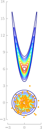
(a)     $\widetilde{T}_{0}$

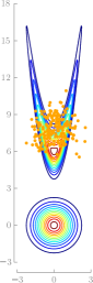
(b)     $\widetilde{T}_{1}$

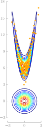
(c)     $\widetilde{T}_{2}$

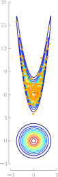
(d)     $\widetilde{T}_{3}$

Figure 1: Computation of a simple transport map in two dimensions: The leftmost figure shows contours of the reference density $\eta$, which is a standard Gaussian, and of the target density $\pi$, which is a banana-shaped distribution in the tails of $\eta$. The target distribution has a nonlinear dependence structure. The orange dots in the leftmost figure correspond to 100 samples $(\bm{x}_{i})$ from $\eta$ and are used to make a sample-average approximation of (3). We adopt the triangular monotone parameterization of (3.4) for the candidate transport map, where the functions $a_{k},b_{k}$ are expanded in a multivariate Hermite polynomial basis of total degree two [121]. The resulting optimization problem is solved with a quasi-Newton method (BFGS). The $k$th figure from the left shows the pushforward of the original reference samples through the approximate transport map, $\widetilde{T}_{k}$, after $k$ iterations of BFGS. The initial map $\widetilde{T}_{0}$ is chosen to be the identity. The reference samples flow collectively towards the target density and eventually settle on the support of $\pi$, capturing its structure after just a few iterations.

4 Markov networks

Let $\bm{Z}=(Z_{1},\ldots,Z_{n})$ be a collection of random variables with law $\bm{\nu}_{\pi}$ and density $\pi$. We can represent a list of conditional independences satisfied by $\bm{Z}$—the so-called Markov properties—using a simple undirected graph $\bm{\mathcal{G}}=(\mathcal{V},\mathcal{E})$, where each node $k\in\mathcal{V}$ is associated with a distinct random variable, $Z_{k}$, and where the edges in $\mathcal{E}$ encode a specific notion of probabilistic interaction among these random variables [62]. In particular, we say that $\bm{Z}$ is a Markov network—or a Markov random field (MRF)—with respect to $\bm{\mathcal{G}}$ if for any triplet $\mathcal{A},\mathcal{S},\mathcal{B}$ of disjoint subsets of $\mathcal{V}$, where $\mathcal{S}$ is a separator set for $\mathcal{A}$ and $\mathcal{B}$, the subcollections $\bm{Z}_{\mathcal{A}}$ and $\bm{Z}_{\mathcal{B}}$ are conditionally independent given $\bm{Z}_{\mathcal{S}}$, i.e.,

$$\bm{Z}_{\mathcal{A}}\perp\!\!\!\perp\bm{Z}_{\mathcal{B}}\,|\,\bm{Z}_{\mathcal{S}}.$$ (4.1)

The measure $\bm{\nu}_{\pi}$ is said to satisfy the global Markov property, relative to $\bm{\mathcal{G}}$, if (4.1) holds [65]. We can also say that $\bm{\nu}_{\pi}$ is globally Markov with respect to $\bm{\mathcal{G}}$. The corresponding graph is then called an independence map (I-map) for $\bm{\nu}_{\pi}$ [62].

Intuitively, a sparse graph represents a family of distributions that enjoy many conditional independence properties. I-maps are in general not unique. Of particular interest are minimal I-maps, i.e., the sparsest graphs compatible with the conditional independence structure of $\bm{\nu}_{\pi}$.

Conditional independence is associated with factorization properties of $\pi$. For instance, $\bm{Z}_{\mathcal{A}}\perp\!\!\!\perp\bm{Z}_{\mathcal{B}}\,|\,\bm{Z}_{\mathcal{S}}$ if and only if $\pi_{\bm{Z}_{\mathcal{A}},\bm{Z}_{\mathcal{B}}|\bm{Z}_{\mathcal{S}}}=\pi_{\bm{Z}_{\mathcal{A}}|\bm{Z}_{\mathcal{S}}}\,\pi_{\bm{Z}_{\mathcal{B}}|\bm{Z}_{\mathcal{S}}}$ a.e. [65]. We then say that $\bm{\nu}_{\pi}$ factorizes according to some graph $\bm{\mathcal{G}}$ if there exists a version of the density of $\bm{\nu}_{\pi}$ such that

$$\pi(\bm{z})=\frac{1}{\mathfrak{c}}\prod_{\mathcal{C}\in\bm{\mathcal{C}}}\,\psi_{\mathcal{C}}(\bm{z}_{\mathcal{C}}),$$ (4.2)

for some nonnegative functions $(\psi_{\mathcal{C}})$ called potentials, where $\bm{\mathcal{C}}$ is the set of maximal cliques of $\bm{\mathcal{G}}$ and $\mathfrak{c}$ is a normalizing constant. It is immediate to show that if $\bm{\nu}_{\pi}$ factorizes according to $\bm{\mathcal{G}}$, then $\bm{\nu}_{\pi}$ satisfies the global Markov property relative to $\bm{\mathcal{G}}$ [65, Proposition 3.8]. The converse is true only under additional assumptions: for instance, if $\bm{\nu}_{\pi}$ admits a continuous and strictly positive density (see the Hammersley-Clifford theorem [47, 65]).

A critical question then is how to characterize a suitable I-map for a given measure. There are several answers. First of all, in many applications that involve probabilistic modeling, the target distribution is defined in terms of its potentials, as in (4.2), because this is just a more convenient way to specify a high-dimensional distribution and to perform inference (or general probabilistic reasoning) with it [62]. Finding a graph for which $\bm{\nu}_{\pi}$ factorizes is then a trivial task. See Figure 4 (left) for an example. Applications where this commonly holds range from spatial statistics and image analysis to speech recognition [62, 99]. In Section 7, for example, we focus exclusively on discrete-time Markov processes, where the Markov structure of the problem is self-evident. More specifically, Section 7 tackles the problem of recursive smoothing and static parameter estimation for a state-space model. In this context, the target measure $\bm{\nu}_{\pi}$ could represent the joint distribution of state and parameters, conditioned on all the available observations (see Figures 4 and 8). The reader might want to consider this sequential inference problem as a guiding application while reading the forthcoming Sections 5 and 6. We emphasize, however, that our theory is far more general and by no means restricted to any specific Markov structure.

In other settings, the graph is unknown and must be estimated. When only samples from $\bm{\nu}_{\pi}$ are available, this is a question of model learning, as described in [62, Part III]; see also [51, 74, 124, 67] for various applications. In case of a known and smooth target density, we can characterize pairwise conditional independence in terms of mixed second-order partial derivatives, as shown by the following lemma.

Lemma 4.1 (Pairwise conditional independence).

If $\bm{Z}\sim\bm{\nu}_{\pi}$ for a measure $\bm{\nu}_{\pi}$ with smooth and strictly positive density $\pi$, we have:

$$Z_{i}\perp\!\!\!\perp Z_{j}\,|\,\bm{Z}_{\mathcal{V}\setminus(i,j)}\quad\Longleftrightarrow\quad\partial^{2}_{i,j}\log\pi=0\,\,{\text{o}n}\,\,\mathbb{R}^{n}.$$ (4.3)

Thus, if we can evaluate $\pi$ and its derivatives (up to a normalizing constant), we can use Lemma 4.1 to assess pairwise conditional independence and to define a minimal I-map for $\bm{\nu}_{\pi}$ as follows: add an edge between every pair of distinct nodes unless the corresponding random variables are conditionally independent [62, Theorem 4.5].

Regardless of the many ways to obtain an I-map, there is a fundamental connection between Markov properties of a distribution and the existence of low-dimensional transport maps. The rest of the paper will elaborate precisely on this connection.

5 Sparsity of triangular transport maps

We begin our investigation of low dimensional structure by considering the notion of sparse transport map. A sparse map is a multivariate function where each component does not depend on all of its input variables. According to this definition, a triangular transport is already sparse. In this section, however, we show that the KR rearrangement can be even sparser, depending on the Markov structure of the target distribution.

5.1 Sparsity bounds

Given a lower triangular function $T$, we define its sparsity pattern, $\mathfrak{I}_{T}$, as the set of all integer pairs $(j,k)$, with $j<k$, such that the $k$th component of the map does not depend on the $j$th input variable, i.e., $\mathfrak{I}_{T}=\{(j,k):j<k,\,\partial_{j}T^{k}=0\}$. (We do not include pairs $j>k$ in the definition of $\mathfrak{I}_{T}$ since, for a lower triangular function, $\partial_{j}\,T^{k}=0$ for $j>k$ by construction.)

Knowing the sparsity pattern of the KR rearrangement before computing the actual transport has important computational implications. For instance, in the variational characterization of the transport described in (3), we can restrict the feasible domain to the set of triangular maps with sparsity pattern given by $\mathfrak{I}_{T}$, and still recover the desired KR rearrangement. That is, if $(j,k)\in\mathfrak{I}_{T}$, we can parameterize any candidate transport map by removing the dependence on the $j$th input variable from the $k$th component of the map. Thus, analyzing the Markov structure of the target distribution enables the representation and computation of maps in possibly higher-dimensional settings.

The following theorem, which is the main result of this section, characterizes bounds on the sparsity patterns of triangular transport maps given an I-map for the target measure. In the statement of the theorem, we denote the direct transport by $T$ and the inverse transport by $S=T^{-1}$ (see Section 3). The theorem suggests that $S$ and $T$ can have quite different sparsity patterns.

Theorem 5.1 (Sparsity of Knothe–Rosenblatt rearrangements).

Let $\bm{X}\sim\bm{\nu}_{\eta}$, $\bm{Z}\sim\bm{\nu}_{\pi}$ with $\bm{\nu}_{\eta},\bm{\nu}_{\pi}\in\mathscr{M}_{+}(\mathbb{R}^{n})$ and $\bm{\nu}_{\eta}$ a product measure on $\times_{i=1}^{n}\mathbb{R}$. Moreover, assume that $\bm{\nu}_{\pi}$ is globally Markov with respect to $\bm{\mathcal{G}}$, and define, recursively, the sequence of graphs $(\bm{\mathcal{G}}^{k})_{k=1}^{n}$ as: (1) $\bm{\mathcal{G}}^{n}\coloneqq\bm{\mathcal{G}}$ and (2) for all $1\leq k<n$, $\bm{\mathcal{G}}^{k-1}$ is obtained from $\bm{\mathcal{G}}^{k}$ by removing node $k$ and by turning its neighborhood ${\rm Nb}(k,\bm{\mathcal{G}}^{k})$ into a clique. Then the following hold:

1. If $\mathfrak{I}_{S}$ is the sparsity pattern of the inverse transport map $S$, then

   $$\widehat{\mathfrak{I}}_{S}\subset\mathfrak{I}_{S},$$ (5.1)

   where $\widehat{\mathfrak{I}}_{S}$ is the set of integer pairs $(j,k)$ such that $j\notin{\rm Nb}(k,\bm{\mathcal{G}}^{k})$.

2. If $\mathfrak{I}_{T}$ is the sparsity pattern of the direct transport map $T$, then

   $$\widehat{\mathfrak{I}}_{T}\subset\mathfrak{I}_{T},$$ (5.2)

   where $\widehat{\mathfrak{I}}_{T}$ is defined recursively as follows: for $k=2,\ldots,n$ the pair $(j,k)\in\widehat{\mathfrak{I}}_{T}$ if and only if $(j,i)\in\widehat{\mathfrak{I}}_{T}$ for all $i\in{\rm Nb}(k,\bm{\mathcal{G}}^{k})$.

3. The predicted sparsity pattern of $S$ is always greater than or equal to that of $T$, i.e.,

   $$\widehat{\mathfrak{I}}_{T}\subset\widehat{\mathfrak{I}}_{S}.$$ (5.3)

Several remarks are in order. First, we emphasize the fact that Theorem 5.1 characterizes sparsity patterns using only an I-map for $\bm{\nu}_{\pi}$, without requiring any actual computation of the transports. One only needs to perform simple graph operations on $\bm{\mathcal{G}}$ to build the sequence of graphs $(\bm{\mathcal{G}}^{k})$. See Figure 2 for an illustration of this procedure, with the corresponding sparsity patterns in Figure 3. We refer to $(\bm{\mathcal{G}}^{k})$ as the marginal graphs. In fact, the sequence $(\bm{\mathcal{G}}^{k})$ is precisely the set of intermediate graphs produced by the variable elimination algorithm [62, Ch. 9], when marginalizing with elimination ordering $(n,n-1,\ldots,1)$. This should not be surprising as the KR rearrangement is essentially a sequence of ordered marginalizations [117]. The hypothesis that $\bm{\nu}_{\eta}$ is a product measure is important for the theorem to hold. If we pick a reference measure with an arbitrary Markov structure, there need not exist a sparse transport map coupling $\bm{\nu}_{\eta}$ and $\bm{\nu}_{\pi}$, even if $\bm{\nu}_{\pi}$ has a sparse I-map. The role of a reference measure is somewhat peculiar to the world of couplings and is usually not addressed in classical treatments of graphical models. Nonetheless, this assumption on $\bm{\nu}_{\eta}$ is not restrictive in the present framework, since the reference distribution is considered a degree of freedom of the problem. Theorem 5.1 gives sufficient but not necessary conditions on $(\bm{\nu}_{\eta},\bm{\nu}_{\pi})$ for the existence of a sparse map. And it could not be otherwise: if $\bm{\nu}_{\eta}=\bm{\nu}_{\pi}$ then the identity map—the sparsest possible map—would be a valid coupling.

We also note that Theorem 5.1 does not provide the exact sparsity patterns of the triangular transport maps; instead, (5.1) and (5.2) provide subsets of $\mathfrak{I}_{T}$ and $\mathfrak{I}_{S}$. In other words, the actual transport maps might be sparser than predicted by the sets $\widehat{\mathfrak{I}}_{S}$ and $\widehat{\mathfrak{I}}_{T}$—but, crucially, they cannot be less sparse. Thus, we can think of Theorem 5.1 as providing bounds on the sparsity of triangular transports. An important fact is that, without additional information on $\bm{\nu}_{\pi}$, these bounds are sharp. That is, we can always find a pair of measures $(\bm{\nu}_{\eta},\bm{\nu}_{\pi})$ satisfying the hypotheses of Theorem 5.1 and such that the predicted and actual sparsity patterns coincide, i.e., $\widehat{\mathfrak{I}}_{T}=\mathfrak{I}_{T}$ or $\widehat{\mathfrak{I}}_{S}=\mathfrak{I}_{S}$.

Part 3 of Theorem 5.1 shows that the predicted sparsity pattern of the inverse KR rearrangement is always larger than or equal to that of the direct transport, i.e., $\widehat{\mathfrak{I}}_{T}\subset\widehat{\mathfrak{I}}_{S}$. This does not mean that for every pair of measures $(\bm{\nu}_{\eta},\bm{\nu}_{\pi})$, the inverse triangular transport is always at least as sparse as the direct transport; in fact, it is possible to provide simple counterexamples. However, this result does imply that if we are only given an I-map for $\bm{\nu}_{\pi}$, then parameterizing candidate inverse triangular transports allows the imposition of more sparsity constraints than parameterizing candidate direct transports. In general, sparser transports are easier to represent. See Figure 4 (right) for a nontrivial example of sparsity patterns for a stochastic volatility model.

Indeed, (5.3) hints at a typical trend: inverse transport maps tend to be sparser (in many practical cases, much sparser) than their direct counterparts. Intuitively, the sparsity of a direct transport is associated with marginal independence in $\bm{Z}$, whereas the inverse transport inherits sparsity from the conditional independence structure of $\bm{Z}$. The latter is a weaker condition than mutual independence; for instance, the correlation length of a process modeled by a Markov random field may be much larger than the typical neighborhood size [99, 8]. Thus, given a sparse I-map for the target measure, it can be computationally advantageous to characterize an inverse transport rather than a direct one, because the inverse transport can inherit a larger sparsity pattern. Given an inverse triangular transport $S$, we can then easily evaluate the direct transport $T=S^{-1}$ at any point $\bm{x}\in\mathbb{R}^{n}$ by inverting $S$ pointwise, as described in Section 3. There is no need to have an explicit representation of the direct transport as long as it can be implicitly defined through its inverse.

(a) $\bm{\mathcal{G}}^{5}$

(b) $\bm{\mathcal{G}}^{4}$

(c) $\bm{\mathcal{G}}^{3}$

(d) $\bm{\mathcal{G}}^{2}$

Figure 2: Sequence of graphs $(\bm{\mathcal{G}}^{k})$ described in Theorem 5.1 for a target measure in $\mathscr{M}_{+}(\mathbb{R}^{5})$ with I-map illustrated by the leftmost graph, $\bm{\mathcal{G}}^{5}$. Notice that to generate the graph $\bm{\mathcal{G}}^{2}$, we remove node $3$ from $\bm{\mathcal{G}}^{3}$ and turn its neighborhood into a clique by adding the edge $(1,2)$.

(a) ${\bf P}_{jk}=\partial_{j}S^{k}$

(b) ${\bf P}_{jk}=\partial_{j}T^{k}$

Figure 3: Sparsity patterns predicted by Theorem 5.1 for the target measure analyzed in Figure 2. We represent the sparsity patterns using a symbolic matrix notation: the $(j,k)$-th entry of the matrix is not colored if the $k$th component of the map ($S$ or $T$) does not depend on the $j$th input variable, or, equivalently, if $(j,k)\in\widehat{\mathfrak{I}}_{S}$ (resp. $\widehat{\mathfrak{I}}_{T}$) (5.1). (Since we are considering lower triangular transports, all entries $j>k$ are uncolored. Note also that $S^{k}$ and $T^{k}$ are always functions of their $k$th input by strict monotonicity of the map.) The predicted sparsity pattern for the direct transport in this example is $\widehat{\mathfrak{I}}_{T}=\emptyset$.

(a)

(b) ${\bf P}_{jk}=\partial_{j}S^{k}$

Figure 4: (left) Markov network for a stochastic volatility model in [57]. Blue nodes represent the discrete-time latent log-volatility process $(\bm{Z}_{k})_{k=0}^{N}$, which obeys a simple autoregressive model with hyperparameters $\bm{\mu},\bm{\phi}$. The graph above is a minimal I-map for the posterior density described in Section 8, $\pi_{\bm{\mu},\bm{\phi},\bm{Z}_{0:N}|\bm{y}_{0:N}}$, where $\bm{y}_{0:N}$ are some (fixed) observations. (right) The predicted sparsity pattern $\widehat{\mathfrak{I}}_{S}$ (only the top $6\times 6$ block is shown) for the inverse transport corresponding to the model on the left: the first column/row of the matrix refer jointly to all of the hyperparameters. Each component $S^{k}$ of the inverse transport can depend at most on four input variables, namely $\bm{\mu},\bm{\phi},\bm{Z}_{k-1},\bm{Z}_{k}$, regardless of the overall dimension $N$ of the problem. In order to apply the results of Theorem 5.1, we must select an ordering of the input variables; here, we used the ordering $(\bm{\mu},\bm{\phi},\bm{Z}_{0},\ldots,\bm{Z}_{N})$. Optimal orderings are further discussed in Section 5.3.

5.2 Connection to Gaussian Markov random fields

The reader familiar with Gaussian Markov random fields (GMRFs), might see links between the preceding results and widespread approaches to the modeling of Gaussian fields. In this section, we clarify the extent of these connections.

Many applications (e.g., image analysis, spatial statistics, time series) involve modeling by means of high-dimensional Gaussian fields. Dealing with large and dense covariances, however, is often impractical; both storage and sampling of the Gaussian field are problematic. The usual workaround is to replace or approximate the Gaussian field with a sparse GMRF—i.e., a Gaussian Markov network that enforces locality in the probabilistic interactions among the underlying random variables. The minimal I-map for the GMRF is thus sparse, and so is the precision matrix $\Lambda$ of the field [99]. The covariance matrix is still in general dense, but dealing with the sparse precision matrix is much easier. If $LL^{\top}$ is a (sparse) Cholesky decomposition of $\Lambda$, then $L^{\top}$ represents a linear triangular transport that pushes forward the joint distribution of the GMRF, $\bm{\nu}_{\pi}=\mathcal{N}(0,\Lambda^{-1})$, to a standard normal, $\bm{\nu}_{\eta}=\mathcal{N}(0,{\bf I})$. The key point is that for many Markov structures of interest, the Cholesky factor inherits sparsity from the underlying graph, so that sampling from $\bm{\nu}_{\pi}$ can be achieved at low cost as follows: if $\bm{X}$ is a sample from $\bm{\nu}_{\eta}$, then we can obtain a sample $\bm{Z}$ from $\bm{\nu}_{\pi}$ simply by solving the sparse triangular linear system $L^{\top}\,\bm{Z}=\bm{X}$. There is no need to explicitly represent or store the dense factor $L^{-\top}$, since we can implicitly represent its action by inverting a sparse triangular function.

Now the connection with Section 5.1 is clear: $L^{\top}$ is an inverse triangular transport, while $L^{-\top}$ is a direct one. Moreover, solving a triangular linear system is just a particular instance of inverting a nonlinear triangular function by performing a sequence of one-dimensional root-findings. Thus the developments of the previous section, which consider arbitrary nonlinear maps, are a natural generalization—to the non-Gaussian case—of modeling and sampling techniques for high-dimensional GMRFs [99].

5.3 Ordering of triangular maps

The results of Theorem 5.1 suggest that the sparsity of a triangular transport map depends on the ordering of the input variables. See Figure 5 for a simple illustration. Indeed, the triangular transport itself depends anisotropically on the input variables and requires the definition of a proper ordering. A natural approach is then to seek the ordering that promotes the sparsest transport map possible.

Consider a pair of measures $(\bm{\nu}_{\eta},\bm{\nu}_{\pi})$ that satisfies the hypotheses of Theorem 5.1. We associate an ordering of the input variables with a permutation $\sigma$ on $\mathbb{N}_{n}=\{1,\ldots,n\}$, and define the reordered target measure $\bm{\nu}_{\pi}^{\sigma}$ as the pushforward of $\bm{\nu}_{\pi}$ by the matrix $Q^{\sigma}$ that represents the permutation $\sigma$. In particular, $(Q^{\sigma})_{ij}=(\bm{e}_{\sigma(i)})_{j}$, where $\bm{e}_{i}$ is the $i$th standard basis vector on $\mathbb{R}^{n}$. Moreover, if $\bm{\mathcal{G}}$ is an I-map for $\bm{\nu}_{\pi}$, then we denote an I-map for $\bm{\nu}_{\pi}^{\sigma}$ by $\bm{\mathcal{G}}^{\sigma}$. Notice that $\bm{\mathcal{G}}^{\sigma}$ can be derived from $\bm{\mathcal{G}}$ simply by relabeling its nodes according to the permutation $\sigma$. Then we can cast a variational problem for the best ordering $\sigma^{\ast}$ as:

$$\sigma^{*}\in\, {\rm arg\,max_{\sigma}}\quad |\mathfrak{I}_{S}|$$

$${\rm s.t.}\quad S_{\sharp}\,\bm{\nu}_{\pi}^{\sigma}=\bm{\nu}_{\eta}$$

$$\sigma\in\mathfrak{P}(\mathbb{N}_{n}),$$

where $S$ is the KR rearrangement that pushes forward the reordered target $\bm{\nu}_{\pi}^{\sigma}$ to $\bm{\nu}_{\eta}$ and $\mathfrak{P}(\mathbb{N}_{n})$ is the set of permutations of $\mathbb{N}_{n}$. The goal is to maximize the cardinality of the sparsity pattern of the inverse map, $|\mathfrak{I}_{S}|$. We restrict our attention to the sparsity of the inverse transport, since we know from Section 5.1 that the direct transport tends to be dense, even for the most trivial Markov structures.

Ideally, we would like to determine a good ordering for the map before computing the actual transport, and to use the resulting information about the sparsity pattern to simplify the optimization problem for $S$. However, evaluating the objective function of (5.3) requires computing a different inverse transport for each permutation $\sigma$. One possible way to relax (5.3) is to replace $\mathfrak{I}_{S}$ with the predicted sparsity pattern $\widehat{\mathfrak{I}}_{S}$ introduced in (5.1). The advantage of this approach is that the objective function of the relaxed problem can now be evaluated in closed form without computing any transport map, but rather by performing the simple sequence of graph operations on $\bm{\mathcal{G}}^{\sigma}$ described by Theorem 5.1. The caveat is that, in general, $\widehat{\mathfrak{I}}_{S}\subset\mathfrak{I}_{S}$, and thus maximizing $|\widehat{\mathfrak{I}}_{S}|$ amounts to seeking the tightest lower bound on the sparsity pattern of the inverse transport. From the definition of $\widehat{\mathfrak{I}}_{S}$, it follows that the best ordering $\sigma^{*}$ for the relaxed problem is one that introduces the fewest edges in the construction of the marginal graphs $\bm{\mathcal{G}}^{n},\ldots,\bm{\mathcal{G}}^{1}$, whenever $\bm{\mathcal{G}}^{n}=\bm{\mathcal{G}}^{\sigma^{*}}$. Thus, for a given I-map $\bm{\mathcal{G}}$, we denote by $\textswab{F}(\sigma;\bm{\mathcal{G}})$ the ${\it fill}$-${\it in}$ produced by the ordering $\sigma$. That is, $\textswab{F}(\sigma;\bm{\mathcal{G}})$ is a set containing all the edges introduced in the construction of the marginal graphs $(\bm{\mathcal{G}}^{k})$ from $\bm{\mathcal{G}}^{\sigma}$. A computationally feasible relaxation of (5.3) is then given by:

$$\sigma^{*}\in\, {\rm arg\,min_{\sigma}}\quad |\textswab{F}(\sigma;\bm{\mathcal{G}})|$$

$${\rm s.t.}\quad \sigma\in\mathfrak{P}(\mathbb{N}_{n})\,.$$

(5.3) is a standard problem in graph theory; it arises in a variety of practical settings, including (most relatedly) finding the best elimination ordering for variable elimination in graphical models [62], or finding the permutation that minimizes the fill-in of the Cholesky factor of a positive definite matrix [40, 101]. From an algorithmic point of view, (5.3) is NP-complete [123]. This should not be surprising, as best–ordering problems are typically combinatorial in nature. Nevertheless, given its widespread applicability, a host of effective polynomial-time heuristics for (5.3) have been developed in past years (e.g., min-fill or weighted-min-fill [62]). Most importantly, (5.3) can be solved without ever touching the target measure (assuming, of course, that an I-map $\bm{\mathcal{G}}$ for $\bm{\nu}_{\pi}$ is known). As a result, the cost of finding a good ordering is often negligible compared to the cost of characterizing a nonlinear transport map via optimization.

(a) $\bm{\mathcal{G}}$

(b) ${\bf P}_{ij}=\partial_{i}S^{j}$

(c) $\bm{\mathcal{G}}^{\prime}$

(d) ${\bf P}_{ij}^{\prime}=\partial_{i}S^{j}$

Figure 5: Illustration of how a simple re-ordering of the input variables can change the (predicted) sparsity pattern of the inverse map. On the left, $\bm{\mathcal{G}}$ represents an I-map for the target measure considered in Figure 2, with ordering $(Z_{1},Z_{2},Z_{3},Z_{4},Z_{5})$, together with its sparsity pattern $\widehat{\mathfrak{I}}_{S}$. (See Figure 3 for details on the “matrix” representation of sparsity patterns.) On the right, $\bm{\mathcal{G}}^{\prime}$ is an I-map for the same target measure but with the ordering $(Z_{1},Z_{2},Z_{5},Z_{4},Z_{3})$. The corresponding sparsity pattern $\widehat{\mathfrak{I}}_{S^{\prime}}$ is now the empty set.

6 Decomposability of transport maps

Thus far, we have investigated the sparsity of triangular transport maps and found that inverse transports tend to inherit sparsity from the underlying Markov structure of the target measure. Though direct triangular transports also inherit some sparsity according to Theorem 5.1, they tend to be more dense.

This section shows that direct transports enjoy a different form of low-dimensional structure: decomposability. A decomposable transport map is a function that can be written as the composition of a finite number of low-dimensional maps, e.g., $T=T_{1}\circ\cdots\circ T_{\ell}$ for some integer $\ell\geq 2$. We use a very specific notion of low-dimensional map, as follows.

Definition 6.1 (Low-dimensional map with respect to a set).

A map $M:\mathbb{R}^{n}\rightarrow\mathbb{R}^{n}$ is low-dimensional with respect to a nonempty set $\mathcal{C}\subset\mathcal{V}\simeq\mathbb{N}_{n}$ if

1. $M^{k}(\bm{x})=x_{k}$ for $k\in\mathcal{C}$

2. $\partial_{j}M^{k}=0$ for $j\in\mathcal{C}$ and $k\in\mathcal{V}\setminus\mathcal{C}$.

The effective dimension of $M$ is the minimum cardinality $|\mathcal{V}\setminus\mathcal{C}|$ over all sets $\mathcal{C}$ with respect to which $M$ is low-dimensional.

In particular, up to a permutation of its components, we can rewrite $M$ as:

$$M(\bm{x})=\left[\begin{array}[]{l}M^{\bar{\mathcal{C}}}(\bm{x}_{\bar{\mathcal{C}}})\\ \bm{x}_{\mathcal{C}}\end{array}\right],$$ (6.1)

where $\bar{\mathcal{C}}=\mathcal{V}\setminus\mathcal{C}$ denotes the complement of $\mathcal{C}$ in $\mathcal{V}$, and where for any map $M$ and set $\mathcal{A}=\{a_{1},\ldots,a_{k}\}$, $M^{\mathcal{A}}$ denotes the multivariate function $\bm{x}\mapsto(M^{a_{1}}(\bm{x}),\ldots,M^{a_{k}}(\bm{x}))$ obtained by stacking together the components of $M$ with index in $\mathcal{A}$. Thus $M$ is the trivial embedding of a $|\bar{\mathcal{C}}|$-dimensional function into the identity map and has effective dimension bounded by $|\bar{\mathcal{C}}|<n$. It is not surprising, then, that a decomposable transport $T=T_{1}\circ\cdots\circ T_{\ell}$ should be easier to represent than an ordinary map. A perhaps less intuitive feature, however, is that the computation of a high-dimensional decomposable transport can be broken down into multiple simpler steps, each associated with the computation of a low-dimensional map $T_{j}$ that accounts only for local features of the target measure.

The forthcoming analysis will consider general, and hence possibly non-triangular, transports. Thus its scope is much broader than that of Section 5, where we only focused on the sparsity of triangular transports. Yet, we will show that triangular maps are the building block of decomposable transports. The cornerstone of our analysis is Theorem 6.1, which characterizes the existence and structure of decomposable transports given only the Markov structure of the underlying target measure.

Our discussion will proceed in two stages: first, we show how to identify direct transports that decompose into two maps, i.e., $T=T_{1}\circ T_{2}$, and then we explain how to apply this result recursively to obtain a general decomposition of the form $T=T_{1}\circ\cdots\circ T_{\ell}$.

6.1 Preliminary notions

Before addressing the decomposability of transport maps, we need to introduce two useful concepts: proper graph decompositions and generalized triangular functions. The decomposition of a graph is a standard notion [65].

Definition 6.2 (Proper graph decomposition).

Given a graph $\bm{\mathcal{G}}=(\mathcal{V},\mathcal{E})$, a triple $(\mathcal{A},\mathcal{S},\mathcal{B})$ of disjoint subsets of the vertex set $\mathcal{V}$ forms a proper decomposition of $\bm{\mathcal{G}}$ if (1) $\mathcal{V}=\mathcal{A}\cup\mathcal{S}\cup\mathcal{B}$, (2) $\mathcal{A}$ and $\mathcal{B}$ are nonempty, (3) $\mathcal{S}$ separates $\mathcal{A}$ from $\mathcal{B}$, and (4) $\mathcal{S}$ is a clique.

See Figure 6 (top left) for an example of a decomposition. Clearly, not every graph admits a proper decomposition; for instance, a fully connected graph does not have a separator set for nonempty $\mathcal{A}$ and $\mathcal{B}$. The idea we will pursue here is that graph decompositions lead to the existence of decomposable transports.

The notion of a generalized triangular function is perhaps less standard, but still relatively straightforward:

Definition 6.3 (Generalized triangular function).

A function $T:\mathbb{R}^{n}\rightarrow\mathbb{R}^{n}$ is said to be generalized triangular, or simply $\sigma$-triangular, if there exists a permutation $\sigma$ of $\mathbb{N}_{n}$ such that the $\sigma(k)$th component of $T$ depends only on the variables $x_{\sigma(1)},\ldots,x_{\sigma(k)}$, i.e., $T^{\sigma(k)}(\bm{x})=T^{\sigma(k)}(x_{\sigma(1)},\ldots,x_{\sigma(k)})$ for all $\bm{x}=(x_{1},\ldots,x_{n})$ and for all $k=1,\ldots,n$.

We can think of a generalized triangular function as a map that is lower triangular up to a permutation. In particular, if $\sigma$ is the identity on $\mathbb{N}_{n}$, then a $\sigma$-triangular function is simply a lower triangular map (see Section 3). To represent the permutation $\sigma$, we use the notation $\sigma(\{i_{1},\ldots,i_{k}\})=\{\sigma(i_{1}),\ldots,\sigma(i_{k})\}$ to denote an ordered set that collects the action of the permutation on the elements $(i_{j})$. For example, if $T:\mathbb{R}^{4}\rightarrow\mathbb{R}^{4}$ is a $\sigma$-triangular map with $\sigma$ defined as $\sigma(\mathbb{N}_{4})=\{1,4,2,3\}$, then $T$ will be of the form:

$$T(\bm{x})=\left[\begin{array}[]{l}T^{1}(x_{1})\\ T^{2}(x_{1},x_{4},x_{2})\\ T^{3}(x_{1},x_{4},x_{2},x_{3})\\ T^{4}(x_{1},x_{4})\end{array}\right]$$ (6.2)

for some collection $(T^{k})$. We regard each component $T^{\sigma(k)}$ as a map $\mathbb{R}^{k}\rightarrow\mathbb{R}$. We say that a $\sigma$-triangular function $T$ is monotone increasing if each component $T^{k}$ is a monotone increasing function of the input $x_{k}$. Moreover, for any $\bm{\nu}_{\eta},\bm{\nu}_{\pi}\in\mathscr{M}_{+}(\mathbb{R}^{n})$ and for any permutation $\sigma$ of $\mathbb{N}_{n}$, there exists a ($\bm{\nu}_{\eta}$-unique) monotone increasing $\sigma$-triangular map—which we call a $\sigma$-generalized KR rearrangement—that pushes forward $\bm{\nu}_{\eta}$ to $\bm{\nu}_{\pi}$. We give a constructive definition for a generalized KR rearrangement in Appendix A.

A key property of a $\sigma$-generalized KR rearrangement is that it allows different sparsity patterns to be engineered, depending on $\sigma$, in a map that is otherwise fully general—in the sense of being able to couple arbitrary measures in $\mathscr{M}_{+}(\mathbb{R}^{n})$. This feature will be essential to characterizing decomposable transport maps.

6.2 Decomposition and graph sparsification

We now characterize transports that decompose into a pair of low-dimensional maps, as described in the following theorem. We formulate the theorem for a generic target measure $\bm{\nu}_{i}$. Later we will apply the theorem recursively to a sequence $(\bm{\nu}_{i})$ of different targets.

Theorem 6.1 (Decomposition of transport maps).

Let $\bm{X}\sim\bm{\nu}_{\eta}$, $\bm{Z}^{i}\sim\bm{\nu}_{i}$, with $\bm{\nu}_{\eta},\bm{\nu}_{i}\in\mathscr{M}_{+}(\mathbb{R}^{n})$ and $\bm{\nu}_{\eta}$ tensor product measure. Denote by $\eta,\pi_{i}$ a pair of nonvanishing densities for $\bm{\nu}_{\eta}$ and $\bm{\nu}_{\pi}$, respectively, and assume that $\bm{\nu}_{i}$ factorizes according to a graph $\bm{\mathcal{G}}^{i}$, which admits a proper decomposition $(\mathcal{A},\mathcal{S},\mathcal{B})$. Then the following hold:

1. There exists a factorization of $\pi_{i}$ of the form

   $$\pi_{i}(\bm{z})=\frac{1}{\mathfrak{c}}\,\psi_{\mathcal{A}\cup\mathcal{S}}(\bm{z}_{\mathcal{A}\cup\mathcal{S}})\,\psi_{\mathcal{S}\cup\mathcal{B}}(\bm{z}_{\mathcal{S}\cup\mathcal{B}}),$$ (6.3)

   where $\psi_{\mathcal{A}\cup\mathcal{S}}$ is strictly positive and integrable, with $\mathfrak{c}=\int\psi_{\mathcal{A}\cup\mathcal{S}}$.

2. For any factorization (6.3) and for any permutation $\sigma$ of $\mathbb{N}_{n}$ with

   $$\sigma(k)\in\begin{cases}\mathcal{S}&\mbox{if }k=1,\ldots,|\mathcal{S}|\\ \mathcal{A}&\mbox{if }k=|\mathcal{S}|+1,\ldots,|\mathcal{A}\cup\mathcal{S}|\\ \mathcal{B}&\mbox{otherwise},\end{cases}$$ (6.4)

   there exists a nonempty family, $\mathfrak{D}_{i}$, of decomposable transport maps $T=L_{i}\circ R$ parameterized by $R\in\mathfrak{R}_{i}$ such that each $T\in\mathfrak{D}_{i}$ pushes forward $\bm{\nu}_{\eta}$ to $\bm{\nu}_{i}$ and where:

   1. $L_{i}$ is a $\sigma$-generalized KR rearrangement that pushes forward $\bm{\nu}_{\eta}$ to a measure with density $\psi_{\mathcal{A}\cup\mathcal{S}}(\bm{z}_{\mathcal{A}\cup\mathcal{S}})\,\eta_{\bm{X}_{\mathcal{B}}}(\bm{z}_{\mathcal{B}})/\mathfrak{c}$ and is low-dimensional with respect to $\mathcal{B}$.

   2. $\mathfrak{R}_{i}$ is the set of maps $\mathbb{R}^{n}\rightarrow\mathbb{R}^{n}$ that are low-dimensional with respect to $\mathcal{A}$ and that push forward $\bm{\nu}_{\eta}$ to the pullback $L_{i}^{\sharp}\,\bm{\nu}_{i}\in\mathscr{M}_{+}(\mathbb{R}^{n})$.

   3. If $\bm{Z}^{i+1}\sim L_{i}^{\sharp}\,\bm{\nu}_{i}$, then $\bm{Z}^{i+1}_{\mathcal{A}}\perp\!\!\!\perp\bm{Z}^{i+1}_{\mathcal{S}\cup\mathcal{B}}$ and $\bm{Z}^{i+1}_{\mathcal{A}}=\bm{X}_{\mathcal{A}}$ in distribution.

   4. $L_{i}^{\sharp}\,\bm{\nu}_{i}$ factorizes according to a graph $\bm{\mathcal{G}}^{i+1}$ that can be derived from $\bm{\mathcal{G}}^{i}$ as follows:

      • Remove any edge from $\bm{\mathcal{G}}^{i}$ that is incident to any node in $\mathcal{A}$.

      • For any maximal clique $\mathcal{C}\subset\mathcal{S}\cup\mathcal{B}$ with nonempty intersection $\mathcal{C}\cap\mathcal{S}$, let $j_{\mathcal{C}}$ be the maximum integer $j$ such that $\sigma(j)\in\mathcal{C}\cap\mathcal{S}$ and turn $\mathcal{C}\cup\{\sigma(1),\ldots,\sigma(j_{\mathcal{C}})\}$ into a clique.

We first look at the theorem for $i=1$ and let $\bm{\nu}_{1}\coloneqq\bm{\nu}_{\pi}$ and $\bm{\mathcal{G}}^{1}\coloneqq\bm{\mathcal{G}}$, where $\bm{\nu}_{\pi}$ denotes our usual target measure with I-map $\bm{\mathcal{G}}$ and where $(\mathcal{A},\mathcal{S},\mathcal{B})$ denotes a decomposition of $\bm{\mathcal{G}}$.

Among the infinitely many transport maps from $\bm{\nu}_{\eta}$ to $\bm{\nu}_{\pi}$, Theorem 6.1 identifies a family of decomposable ones. The existence of these maps relies exclusively on the Markov structure of $\bm{\nu}_{\pi}$: we just require $\bm{\mathcal{G}}$ to admit a (proper) decomposition.

Each transport $T\in\mathfrak{D}_{1}$ pushes forward $\bm{\nu}_{\eta}$ to $\bm{\nu}_{\pi}$ and is the composition of two low-dimensional maps, i.e., $T=L_{1}\circ R$ for a fixed $L_{1}$ defined in Theorem 6.1[Part 2a] and for some $R\in\mathfrak{R}_{1}$. (We also write $\mathfrak{D}_{1}\coloneqq L_{1}\circ\mathfrak{R}_{1}$.) The structure of these low-dimensional maps is quite interesting. Up to a reordering of their components, Theorem 6.1[Parts 2a and 2b] show that $L_{1}$ and $R$ have an intuitive complementary form:

$$L_{1}(\bm{x})=\left[\begin{array}[]{l}L_{1}^{\mathcal{A}}(\bm{x}_{\mathcal{S}},\bm{x}_{\mathcal{A}})\\[2.0pt] L_{1}^{\mathcal{S}}(\bm{x}_{\mathcal{S}})\\[2.0pt] \bm{x}_{\mathcal{B}}\end{array}\right],\qquad R(\bm{x})=\left[\begin{array}[]{l}\bm{x}_{\mathcal{A}}\\[2.0pt] R^{\mathcal{S}}(\bm{x}_{\mathcal{S}},\bm{x}_{\mathcal{B}})\\[2.0pt] R^{\mathcal{B}}(\bm{x}_{\mathcal{S}},\bm{x}_{\mathcal{B}})\end{array}\right].$$ (6.5)

(If $\mathcal{S}=\emptyset$, one can just remove $L_{1}^{\mathcal{S}}$ and $R^{\mathcal{S}}$ from (6.5), and drop the dependence of the remaining components on $\bm{x}_{\mathcal{S}}$.) In particular, $L_{1}$ and $R$ have effective dimensions bounded by $|\mathcal{A}\cup\mathcal{S}|$ and $|\mathcal{S}\cup\mathcal{B}|=|\mathcal{V}\setminus\mathcal{A}|$, respectively (see Definition 6.1). Even though $L_{1}$ and $R$ are low-dimensional maps, their composition is quite dense—in the sense of Section 5—and is in general nontriangular:

$$T(\bm{x})=(L_{1}\circ R)(\bm{x})=\left[\begin{array}[]{l}L_{1}^{\mathcal{A}}(\,R^{\mathcal{S}}(\bm{x}_{\mathcal{S}},\bm{x}_{\mathcal{B}}),\,\bm{x}_{\mathcal{A}})\\[2.0pt] L_{1}^{\mathcal{S}}(\,R^{\mathcal{S}}(\bm{x}_{\mathcal{S}},\bm{x}_{\mathcal{B}})\,)\\[2.0pt] R^{\mathcal{B}}(\bm{x}_{\mathcal{S}},\bm{x}_{\mathcal{B}})\end{array}\right],$$ (6.6)

and thus more difficult to represent and to work with. The key idea of decomposable transports is that they can be represented implicitly through the composition of their low-dimensional factors, similar to the way that direct transports can be represented implicitly through their sparse inverses (Section 5).

The sparsity patterns of $L_{1}$ and $R$ in (6.5) are needed for the theorem to hold. In particular, $L_{1}$ must be a $\sigma$-triangular function with $\sigma$ specified by (6.4). Notice that (6.4) does not prescribe an exact permutation, but just a few constraints on a feasible $\sigma$. Intuitively, these constraints say that $L_{1}$ should be a function whose components with indices in $\mathcal{S}$ depend only on the variables in $\mathcal{S}$ (whenever $\mathcal{S}\neq\emptyset$), and whose components with indices in $\mathcal{A}$ depend only on the variables in $\mathcal{A}\cup\mathcal{S}$. Thus, there is usually some freedom in the choice of $\sigma$. Different permutations lead to different families of decomposable transports, and can induce different sparsity patterns in an I-map, $\bm{\mathcal{G}}^{2}$, for $L_{1}^{\sharp}\,\bm{\nu}_{\pi}$ (Theorem 6.1[Part 2d]).

Part 2d of the theorem shows how to derive a possible I-map $\bm{\mathcal{G}}^{2}$—not necessarily minimal—by performing a sequence of graph operations on $\bm{\mathcal{G}}$. There are two steps: one that does not depend on $\sigma$ and one that does. Let us focus first on the former: the idea is to remove from $\bm{\mathcal{G}}$ any edge that is incident to any node in $\mathcal{A}$, effectively disconnecting $\mathcal{A}$ from the rest of the graph. That is, if $\bm{Z}^{2}\sim L_{1}^{\sharp}\bm{\nu}_{\pi}$, then, regardless of $\sigma$, $L_{1}$ makes $\bm{Z}_{\mathcal{A}}^{2}$ marginally independent of $\bm{Z}_{\mathcal{S}\cup\mathcal{B}}^{2}$ by acting locally on $\bm{\mathcal{G}}$. And not only that: $L_{1}$ also ensures that the marginals of $\bm{\nu}_{\eta}$ and $L_{1}^{\sharp}\bm{\nu}_{\pi}$ agree along $\mathcal{A}$ (see Theorem 6.1[Part 2c]). Thus we should really interpret $L_{1}$ as the first step towards a progressive transport of $\bm{\nu}_{\eta}$ to $\bm{\nu}_{\pi}$. $L_{1}$ is a local map: it can depend nontrivially only upon variables in $\bm{x}_{\mathcal{A}\cup\mathcal{S}}$. Indeed, in the most general case, $|\mathcal{A}\cup\mathcal{S}|$ is the minimum effective dimension of a low-dimensional map necessary to decouple $\mathcal{A}$ from the rest of the graph. The more edges incident to $\mathcal{A}$, the higher-dimensional a transport is needed. This type of graph sparsification requires a peculiar “block triangular” structure for $L_{1}$ as shown by (6.5): any $\sigma$-triangular function with $\sigma$ given by (6.4) achieves this special structure. The second step of Part 2d shows that if $\mathcal{S}\neq\emptyset$, then it might be necessary to add edges to the subgraph $\bm{\mathcal{G}}_{\mathcal{S}\cup\mathcal{B}}$, depending on $\sigma$. The relevant aspect of $\sigma$ for this discussion is the definition of the permutation onto the first $|\mathcal{S}|$ integers. In general, there are $|\mathcal{S}|!$ different permutations that could induce different sparsity patterns in $\bm{\mathcal{G}}^{2}$. We shall see that permutations that add the fewest edges possible are of particular relevance.

6.3 Recursive decompositions

The sparsity of $\bm{\mathcal{G}}^{2}$ is important because it affects the “complexity” of the maps in $\mathfrak{R}_{1}$: each $R\in\mathfrak{R}_{1}$ pushes forward $\bm{\nu}_{\eta}$ to $L_{1}^{\sharp}\,\bm{\nu}_{\pi}$. More specifically, by the previous discussion, we can see how the role of each $R\in\mathfrak{R}_{1}$ is really only that of matching the marginals of $\bm{\nu}_{\eta}$ and $L_{1}^{\sharp}\,\bm{\nu}_{\pi}$ along $\mathcal{V}\setminus\mathcal{A}$. A natural question then is whether we can break this matching step into simpler tasks, or, in the language of this section, whether $\mathfrak{R}_{1}$ contains transports that are further decomposable. Intuitively, we are seeking a finer-grained representation for some of the transports in $\mathfrak{R}_{1}$. The following lemma (for $i=1$) provides a positive answer to this question as long as $\mathcal{V}\setminus\mathcal{A}$ is not fully connected in $\bm{\mathcal{G}}^{2}$. From now on, we denote $(\mathcal{A},\mathcal{S},\mathcal{B})$ by $(\mathcal{A}_{1},\mathcal{S}_{1},\mathcal{B}_{1})$, since we will be dealing with a sequence of different graph decompositions.

Lemma 6.1 (Recursive decompositions).

Let $\bm{\nu}_{\eta},\bm{\nu}_{i},\bm{\mathcal{G}}^{i}$ be defined as in the assumptions of Theorem 6.1 for a proper decomposition $(\mathcal{A}_{i},\mathcal{S}_{i},\mathcal{B}_{i})$ of $\bm{\mathcal{G}}^{i}$, while let $\bm{\mathcal{G}}^{i+1}$ and $\mathfrak{D}_{i}=L_{i}\circ\mathfrak{R}_{i}$ be the resulting graph (Part 2d) and family of decomposable transports, respectively. Then there are two possibilities:

1. $\mathcal{S}_{i}\cup\mathcal{B}_{i}$ is not a clique in $\bm{\mathcal{G}}^{i+1}$. In this case, it is possible to identify a proper decomposition $(\mathcal{A}_{i+1},\mathcal{S}_{i+1},\mathcal{B}_{i+1})$ of $\bm{\mathcal{G}}^{i+1}$ for some $\mathcal{A}_{i+1}$ that is a strict superset of $\mathcal{A}_{i}$ by (possibly) adding edges to $\bm{\mathcal{G}}^{i+1}$ in order to turn $\mathcal{S}_{i+1}$ into a clique. Let $\mathfrak{D}_{i+1}=L_{i+1}\circ\mathfrak{R}_{i+1}$ be defined as in Theorem 6.1 for the pair of measures $\bm{\nu}_{\eta},\bm{\nu}_{i+1}\coloneqq L_{i}^{\sharp}\,\bm{\nu}_{i}$ and  $(\mathcal{A}_{i+1},\mathcal{S}_{i+1},\mathcal{B}_{i+1})$. Then the following hold:

   1. $\mathfrak{R}_{i}\supset\mathfrak{D}_{i+1}$ and $L_{i}\circ\mathfrak{R}_{i}\supset L_{i}\circ L_{i+1}\circ\mathfrak{R}_{i+1}$.

   2. $L_{i+1}$ is low-dimensional with respect to $\mathcal{A}_{i}\cup\mathcal{B}_{i+1}$ and has effective dimension bounded by $|(\mathcal{A}_{i+1}\setminus\mathcal{A}_{i})\cup\mathcal{S}_{i+1}|$.

   3. Each $R\in\mathfrak{R}_{i+1}$ has effective dimension bounded by $|\mathcal{V}\setminus\mathcal{A}_{i+1}|$.

2. $\mathcal{S}_{i}\cup\mathcal{B}_{i}$ is a clique in $\bm{\mathcal{G}}^{i+1}$. In this case, the decomposition of Part 1 does not exist.

Lemma 6.1[Part 1] shows that if $\mathcal{S}_{1}\cup\mathcal{B}_{1}$ is not fully connected in $\bm{\mathcal{G}}^{2}$, then there exists a proper decomposition $(\mathcal{A}_{2},\mathcal{S}_{2},\mathcal{B}_{2})$ of $\bm{\mathcal{G}}^{2}$ (obtained, possibly, by adding edges to $\bm{\mathcal{G}}^{2}$ in $\mathcal{V}\setminus\mathcal{A}_{1}$) for which $\mathcal{A}_{2}$ is a strict superset of $\mathcal{A}_{1}$. One can then apply Theorem 6.1 for the pair $\bm{\nu}_{\eta},\bm{\nu}_{2}=L_{1}^{\sharp}\,\bm{\nu}_{1}$ and the decomposition $(\mathcal{A}_{2},\mathcal{S}_{2},\mathcal{B}_{2})$. As a result, Part 1a of the lemma shows that $\mathfrak{R}_{1}$ contains a subset $\mathfrak{D}_{2}=L_{2}\circ\mathfrak{R}_{2}$ of decomposable transport maps where both $L_{2}$ and each $R\in\mathfrak{R}_{2}$ are local transports on $\mathcal{V}\setminus\mathcal{A}_{1}$, i.e., they are both low-dimensional with respect to $\mathcal{A}_{1}$. In particular, $L_{2}$ is responsible for decoupling $\mathcal{A}_{2}\setminus\mathcal{A}_{1}$ from the rest of the graph and for matching the marginals of $\bm{\nu}_{\eta}$ and $L_{2}^{\sharp}\,L_{1}^{\sharp}\,\bm{\nu}_{\pi}=(L_{1}\circ L_{2})^{\sharp}\,\bm{\nu}_{\pi}$ along $\mathcal{A}_{2}\setminus\mathcal{A}_{1}$. The effective dimension of $L_{2}$ is bounded above by the size of the separator set $\mathcal{S}_{2}$ plus the number of nodes in $\mathcal{A}_{2}\setminus\mathcal{A}_{1}$ (Part 1b of the lemma). The effective dimension of each $R\in\mathfrak{R}_{2}$ is bounded by the cardinality of $\mathcal{V}\setminus\mathcal{A}_{2}$ and is, in the most general case, lower than that of the maps in $\mathfrak{R}_{1}$ (Part 1c). Moreover, by Part 1a, $\mathfrak{D}_{1}=L_{1}\circ\mathfrak{R}_{1}\supset L_{1}\circ L_{2}\circ\mathfrak{R}_{2}$, which means that among the infinitely many decomposable transports that push forward $\bm{\nu}_{\eta}$ to $\bm{\nu}_{\pi}$, there exists at least one that factorizes as the composition of three low-dimensional maps as opposed to two, i.e., $T=L_{1}\circ L_{2}\circ R$ for some $R\in\mathfrak{R}_{2}$.

If, on the other hand, $\mathcal{S}_{1}\cup\mathcal{B}_{1}$ is fully connected in $\bm{\mathcal{G}}^{2}$, then by Lemma 6.1[Part 2] we know that the decomposition of Part 1 does not exist. As a result, we cannot use Theorem 6.1 to prove the existence of more finely decomposable transports in $\mathfrak{R}_{1}$. In other words, if we want to match the marginals of $\bm{\nu}_{\eta}$ and $L_{1}^{\sharp}\,\bm{\nu}_{\pi}$ along $\mathcal{V}\setminus\mathcal{A}_{1}=\mathcal{S}_{1}\cup\mathcal{B}_{1}$, then we must do so in one shot, using a single transport map; no more intermediate steps are feasible.

The main idea, then, is to apply Lemma 6.1[Part 1], recursively, $k$ times, where $k$ is the first integer (possibly zero) for which $\mathcal{S}_{k+1}\cup\mathcal{B}_{k+1}$ is a clique in $\bm{\mathcal{G}}^{k+2}$. After $k$ iterations, the following inclusion must hold:

$$\mathfrak{D}_{1}=L_{1}\circ\mathfrak{R}_{1}\supset L_{1}\circ\cdots\circ L_{k+1}\circ\mathfrak{R}_{k+1},$$ (6.7)

which shows that there exists a decomposable transport,

$$T=L_{1}\circ\cdots\circ L_{k+1}\circ R,$$ (6.8)

for some $R\in\mathfrak{R}_{k+1}$, that pushes forward $\bm{\nu}_{\eta}$ to $\bm{\nu}_{\pi}$. (Note that we can apply Lemma 6.1[Part 1] only finitely many times since $|\mathcal{V}\setminus\mathcal{A}_{i+1}|$ is an integer function strictly decreasing in $i$ and bounded away from zero.) Each $L_{i}$ in (6.7) is a $\sigma_{i}$-triangular map for some permutation $\sigma_{i}$ that satisfies (6.8), and is low-dimensional with respect to $\mathcal{A}_{i-1}\cup\mathcal{B}_{i}$, i.e., for $i>1$ and up to a permutation of its components,

$$L_{i}(\bm{x})=\left[\begin{array}[]{l}\bm{x}_{\mathcal{A}_{i-1}}\\[2.0pt] L_{i}^{\mathcal{A}_{i}\setminus\mathcal{A}_{i-1}}(\bm{x}_{\mathcal{S}_{i}},\bm{x}_{\mathcal{A}_{i}\setminus\mathcal{A}_{i-1}})\\[2.0pt] L_{i}^{\mathcal{S}_{i}}(\bm{x}_{\mathcal{S}_{i}})\\[2.0pt] \bm{x}_{\mathcal{B}_{i}}\end{array}\right].$$ (6.9)

The map $R$ is low-dimensional with respect to $\mathcal{A}_{k+1}$ and can also be chosen as a generalized triangular function. Intuitively, we can think of $L_{i}$ as decoupling nodes in $\mathcal{A}_{i}\setminus\mathcal{A}_{i-1}$ from the rest of the graph in an I-map for $(L_{1}\circ\cdots\circ L_{i-1})^{\sharp}\bm{\nu}_{\pi}$. (Recall that by Lemma 6.1 all the sets $(\mathcal{A}_{i})$ are nested, i.e., $\mathcal{A}_{1}\subset\cdots\subset\mathcal{A}_{k+1}$.) Figure 6 illustrates the mechanics underlying the recursive application of Lemma 6.1.

We emphasize that the existence and structure of (6.8) follow from simple graph operations on $\bm{\mathcal{G}}$, and do not entail any actual computation with the target measure $\bm{\nu}_{\pi}$. Notice also that even if each map in the decomposition (6.7) is $\sigma$-triangular, the resulting transport map $T$ need not be triangular at all. In other words, we obtain factorizations of general and possibly non-triangular transport maps in terms of low-dimensional generalized triangular functions. In this sense, we can regard triangular maps as a fundamental “building block” of a much larger class of transport maps.

Decomposable transports are clearly not unique. In particular, there are two factors that affect both the sparsity pattern and the number $k$ of composed maps in the family $L_{1}\circ\cdots\circ L_{k+1}\circ\mathfrak{R}_{k+1}$: the sequence of decompositions $(\mathcal{A}_{i},\mathcal{S}_{i},\mathcal{B}_{i})$ and the sequence of permutations $(\sigma_{i})$. Usually, there is a certain freedom in the choice of these parameters, and each configuration might lead to a different family of decomposable transports. Of course some families might be more desirable than others: ideally, we would like the low-dimensional maps in the composition to have the smallest effective dimension possible. Recall that by Lemma 6.1 the effective dimension of each $L_{i}$ can be bounded above by $|(\mathcal{A}_{i}\setminus\mathcal{A}_{i-1})\cup\mathcal{S}_{i}|$ (with the convention $\mathcal{A}_{0}=\emptyset$). Thus we should intuitively choose a decomposition $(\mathcal{A}_{i},\mathcal{S}_{i},\mathcal{B}_{i})$ of $\bm{\mathcal{G}}^{i}$ and a permutation $\sigma_{i}$ for $L_{i}$ that minimize the cardinality of $(\mathcal{A}_{i}\setminus\mathcal{A}_{i-1})\cup\mathcal{S}_{i}$, and that, at the same time, minimize the number of edges added from $\bm{\mathcal{G}}^{i}$ to $\bm{\mathcal{G}}^{i+1}$. In principle, we should also account for the dimensions of all future maps in the recursion. In the most general case, this graph theoretic question could be addressed using dynamic programming [5]. In practice, however, we will often consider graphs for which a good sequence of decompositions and permutations is rather obvious (see Section 7). For instance, if the target distribution $\bm{\nu}_{\pi}$ factorizes according to a tree $\bm{\mathcal{G}}$, then it is immediate to show the existence of a decomposable transport $T=T_{1}\circ\cdots\circ T_{n-1}$ that pushes forward $\bm{\nu}_{\eta}$ to $\bm{\nu}_{\pi}$ and that factorizes as the composition of $n-1$ low-dimensional maps $(T_{i})_{i=1}^{n-1}$, each associated to an edge of $\bm{\mathcal{G}}$: it suffices to consider a sequence of decompositions $(\mathcal{A}_{i},\mathcal{S}_{i},\mathcal{B}_{i})$ with $\mathcal{A}_{1}\subset\mathcal{A}_{2}\subset\cdots$, where, for a given rooted version of $\bm{\mathcal{G}}$, $\mathcal{A}_{i}\setminus\mathcal{A}_{i-1}$ consists of a single node $a_{i}$ with the largest depth in $\bm{\mathcal{G}}_{\mathcal{V}\setminus\mathcal{A}_{i-1}}$, and where $\mathcal{S}_{i}$ contains the unique parent of that node. Remarkably, each map $T_{i}$ has effective dimension less than or equal to two, independent of $n$—the size of the tree.

At this point, it might be natural to consider a junction tree decomposition of a triangulation of $\bm{\mathcal{G}}$ [62] as a convenient graphical tool to schedule the sequence of decompositions $(\mathcal{A}_{i},\mathcal{S}_{i},\mathcal{B}_{i})$ needed to apply Lemma 6.1 recursively. Decomposable graphs are in fact ultimately chordal [65]. However, the situation might not be as straightforward. The problem is that the clique structure of $\bm{\mathcal{G}}^{i}$, an I-map for $\bm{\nu}_{i}$, can be very different than that of $\bm{\mathcal{G}}^{i+1}$, an I-map for $L_{i}^{\sharp}\,\bm{\nu}_{i}$; Theorem 6.1[Part 2d] shows that $\bm{\mathcal{G}}^{i+1}$ might contain larger maximal cliques than those in $\bm{\mathcal{G}}^{i}$, even if $\bm{\mathcal{G}}^{i}$ is chordal (see Figure 6 for an example). Thus, working with a junction tree might require a bit of extra care.

6.4 Computation of decomposable transports

Given the existence and structure of a decomposable transport like (6.8), what to do with it? There are at least two possible ways of exploiting this type of information. First, one could solve a variational problem like (3) and enforce an explicit parameterization of the transport map as the composition $T=L_{1}\circ\cdots\circ L_{k+1}\circ R$. In this scenario, one need only parameterize the low-dimensional maps $(L_{i},R)$ and optimize, jointly, over their composition. The advantage of this approach is that it bypasses the parameterization of a single high-dimensional function, $T$, altogether. See the literature on normalizing flows [95] for possible computational ideas in this direction.

An alternative—and perhaps more intriguing—possibility is to compute the maps $(L_{i})$ sequentially by solving separate low-dimensional optimization problems—one for each map $L_{i}$. By Theorem 6.1[Part 2a] and Lemma 6.1, there exists a factorization (6.3) of $\pi_{i}$—a density of $L_{i-1}^{\sharp}\,\bm{\nu}_{i-1}$—for which $L_{i}$ is a $\sigma_{i}$-generalized KR rearrangement that pushes forward $\bm{\nu}_{\eta}$ to a measure with density proportional to $\psi_{\mathcal{A}_{i}\cup\mathcal{S}_{i}}\,\eta_{\bm{X}_{\mathcal{B}_{i}}}$, where $(\mathcal{A}_{i},\mathcal{S}_{i},\mathcal{B}_{i})$ is a decomposition of $\bm{\mathcal{G}}^{i}$ and $\bm{\mathcal{G}}^{i}$ is an I-map for $\bm{\nu}_{i}$. In general $\psi_{\mathcal{A}_{i}\cup\mathcal{S}_{i}}$ depends on $L_{i-1}$, and so the maps $(L_{i})$ must be computed sequentially. In essence, decomposable transports break the inference task into smaller and possibly easier steps.

Note that we could define $L_{i}$ with respect to any factorization (6.3) with $\psi_{\mathcal{A}_{i}\cup\mathcal{S}_{i}}$ integrable: these different factorizations would lead to a family of decomposable transports with the same low-dimensional structure and sparsity patterns (as predicted by Theorem 6.1). Thus, as long as we have access to a sequence of integrable factors $(\psi_{\mathcal{A}_{i}\cup\mathcal{S}_{i}})$, we can compute each map $L_{i}$ individually by solving a low-dimensional optimization problem. (See Appendix A for computational remarks on generalized triangular functions.) Intuitively, since by Lemma 6.1[Part 1b] $L_{i}$ is low-dimensional with respect to $\mathcal{A}_{i-1}\cup\mathcal{B}_{i}$, we really only need to optimize for a portion of the map, namely $L_{i}^{\mathcal{C}}$ for $\mathcal{C}=(\mathcal{A}_{i}\setminus\mathcal{A}_{i-1})\cup\mathcal{S}_{i}$, which can be regarded effectively as a multivariate map on $\mathbb{R}^{|\mathcal{C}|}$. In the same way, the map $R$ can be computed as any transport (possibly triangular) that pushes forward $\bm{\nu}_{\eta}$ to $L_{k+1}^{\sharp}\,\bm{\nu}_{k+1}$. Theorem 6.1[Part 2b] tells us that once again we only need to optimize for a low-dimensional portion of the map, namely, $R^{\mathcal{S}_{k+1}\cup\mathcal{B}_{k+1}}$.

While it might be difficult to access a sequence of factorizations (6.3) for a general problem, there are important applications, such as Bayesian filtering, smoothing, and joint parameter/state estimation, where the sequential computation of the transports $(L_{i},R)$ is always possible by construction. We discuss these applications in the next section.

(a)

(b)

(c)

(d)

Figure 6: Sequence of graph decompositions associated with the recursive application of Lemma 6.1. At (top left) is an I-map, $\bm{\mathcal{G}}^{1}$, for $\bm{\nu}_{\pi}$, with $\bm{\nu}_{\pi}\in\mathscr{M}_{+}(\mathbb{R}^{6})$. We first decompose this graph into $(\mathcal{A}_{1},\mathcal{S}_{1},\mathcal{B}_{1})$ as indicated, and apply Theorem 6.1 to the pair $\bm{\nu}_{\eta},\bm{\nu}_{\pi}$. To do so, we first need to add edge $(2,3)$ to $\bm{\mathcal{G}}^{1}$ in order to turn $(\mathcal{A}_{1},\mathcal{S}_{1},\mathcal{B}_{1})$ into a proper decomposition of $\bm{\mathcal{G}}^{1}$ with a fully connected $\mathcal{S}_{1}$.The resulting graph, $\bm{\mathcal{G}}^{1}_{\star}$, is now chordal (in fact, a triangulation of $\bm{\mathcal{G}}^{1}$ [65]), but still an I-map for $\bm{\nu}_{\pi}$. The first map $L_{1}$ is $\sigma_{1}$-triangular with $\sigma_{1}(\mathbb{N}_{6})=\{2,3,1,4,5,6\}$ and it is low-dimensional with respect to $\mathcal{B}_{1}$; The (top right) figure shows the I-map, $\bm{\mathcal{G}}^{2}$, for $L_{1}^{\sharp}\,\bm{\nu}_{\pi}$ as given by Theorem 6.1[Part 2d]: as expected, $\mathcal{A}_{1}$ is disconnected from $\mathcal{S}_{1}\cup\mathcal{B}_{1}$; moreover, a new maximal clique $\{2,3,4,5\}$ appears in $\bm{\mathcal{G}}^{2}$. This new clique is larger than any of the maximal cliques in $\bm{\mathcal{G}}^{1}_{\star}$, even though $\bm{\mathcal{G}}^{1}_{\star}$ is chordal. (Notice that $\sigma_{1}$ is not the permutation that adds the fewest edges possible in $\bm{\mathcal{G}}^{2}$. An example of such “best” permutation would be $\sigma(\mathbb{N}_{6})=\{3,2,1,4,5,6\}$.) Though Theorem 6.1 guarantees the existence of a low-dimensional map $R\in\mathfrak{R}_{1}$ that pushes forward $\bm{\nu}_{\eta}$ to $L_{1}^{\sharp}\,\bm{\nu}_{\pi}$, we instead proceed recursively by applying Lemma 6.1[Part 1] for a proper decomposition, $(\mathcal{A}_{2},\mathcal{S}_{2},\mathcal{B}_{2})$, of $\bm{\mathcal{G}}^{2}$, where $\mathcal{A}_{2}$ is a strict superset of $\mathcal{A}_{1}$ (bottom left). The lemma shows that $\mathfrak{R}_{1}\supset L_{2}\circ\mathfrak{R}_{2}$ for some $\sigma_{2}$-triangular map $L_{2}$, which is low-dimensional with respect to $\mathcal{A}_{1}\cup\mathcal{B}_{2}$, and where each $R\in\mathfrak{R}_{2}$ pushes forward $\bm{\nu}_{\eta}$ to $(L_{1}\circ L_{2})^{\sharp}\bm{\nu}_{\pi}$. Can we apply Lemma 6.1 one more time to characterize decomposable transports in $\mathfrak{R}_{2}$? The answer is no, as the I-map for $(L_{1}\circ L_{2})^{\sharp}\bm{\nu}_{\pi}$ (bottom right) consists of a single clique in $\mathcal{S}_{2}\cup\mathcal{B}_{2}$. Nevertheless, each $R\in\mathfrak{R}_{2}$ is still low-dimensional with respect to $\mathcal{A}_{2}$. Overall, we showed the existence of a transport map $T:\mathbb{R}^{6}\rightarrow\mathbb{R}^{6}$ pushing forward $\bm{\nu}_{\eta}$ to $\bm{\nu}_{\pi}$ that decomposes as $T=L_{1}\circ L_{2}\circ R$, where $L_{1}$, $L_{2}$, $R$ are effectively $\{3,4,3\}$-dimensional maps, respectively.

7 Sequential inference on state-space models: variational algorithms

In this section, we consider the problem of sequential Bayesian inference (or discrete-time data assimilation [66, 94, 104]) for continuous, nonlinear, and non-Gaussian state-space models.

Our goal is to specialize the theory developed in Section 6 to the solution of Bayesian filtering and smoothing problems. The key result of this section is a new variational algorithm for characterizing the full posterior distribution of the sequential inference problem—e.g., not just a few filtering or smoothing marginals—via recursive lag–$1$ smoothing with transport maps. The proposed algorithm builds a decomposable high-dimensional transport map in a single forward pass by solving a sequence of local small-dimensional problems, without resorting to any backward pass on the state space model (see Theorem 7.1). These results extend naturally to the case of joint parameter and state estimation (see Section 7.3 and Theorem 7.2). Pseudocode for the algorithm is given in Appendix C.

A state-space model consists of a pair of discrete-time stochastic processes $(\bm{Z}_{k},\bm{Y}_{k})_{k\geq 0}$ indexed by the time $k$, where $(\bm{Z}_{k})$ is a latent Markov process of interest and where $(\bm{Y}_{k})$ is the observed process. We can think of each $\bm{Y}_{k}$ as a noisy and perhaps indirect measurement of $\bm{Z}_{k}$. The Markov structure corresponding to the joint process $(\bm{Z}_{k},\bm{Y}_{k})$ is shown in Figure 7. The generalization of the results of this section to the case of missing observations is straightforward and will not be addressed here.

We assume that we are given the transition densities $\pi_{\bm{Z}_{k+1}|\bm{Z}_{k}}$ for all $k\geq 0$, sometimes referred to as the “prior dynamic,” together with the marginal density of the initial conditions $\pi_{\bm{Z}_{0}}$. (For instance, the prior dynamic could stem from the discretization of a continuous time stochastic differential equation [81].) We denote by $\pi_{\bm{Y}_{k}|\bm{Z}_{k}}$ the likelihood function, i.e., the density of $\bm{Y}_{k}$ given $\bm{Z}_{k}$, and assume that $\bm{Z}_{k}$ and $\bm{Y}_{k}$ are random variables taking values on $\mathbb{R}^{n}$ and $\mathbb{R}^{d}$, respectively. Moreover, we denote by $(\bm{y}_{k})_{k\geq 0}$ a sequence of realizations of the observed process $(\bm{Y}_{k})$ that will define the posterior distribution over the unobserved (hidden) states of the model, and make the following regularity assumption in our theorems: $\pi_{\bm{Z}_{0:k-1},\bm{Y}_{0:k-1}}>0$ for all $k\geq 1$. (The existence of underlying fully supported measures will be left implicit throughout the section for notational convenience.)

(a)

Figure 7: (above) I-map for the joint process $(\bm{Z}_{k},\bm{Y}_{k})_{k\geq 0}$ defining the state-space model. (below) I-map for the independent reference process $(\bm{X}_{k})_{k\geq 0}$ used in Theorem 7.1.

7.1 Smoothing and filtering: the full Bayesian solution

In typical applications of state-space modeling, the process $(\bm{Y}_{k})$ is only observed sequentially, and thus the goal of inference is to characterize—sequentially in time and via a recursive algorithm—the joint distribution of the current and past states given currently available measurements, i.e.,

$$\pi_{\bm{Z}_{0:k}|\bm{y}_{0:k}}(\bm{z}_{0:k})\coloneqq\pi_{\bm{Z}_{0:k}|\bm{Y}_{0:k}}(\bm{z}_{0:k}|\bm{y}_{0:k})$$ (7.1)

for all $k\geq 0$. That is, we wish to characterize $\pi_{\bm{Z}_{0:k}|\bm{y}_{0:k}}$ based on our knowledge of the posterior distribution at the previous timestep, $\pi_{\bm{Z}_{0:k-1}|\bm{y}_{0:k-1}}$, and with an effort that is constant over time. We regard (7.1) as the full Bayesian solution to the sequential inference problem [104].

Usually, the task of updating $\pi_{\bm{Z}_{0:k-1}|\bm{y}_{0:k-1}}$ to yield $\pi_{\bm{Z}_{0:k}|\bm{y}_{0:k}}$ becomes increasingly challenging over time due to the widening inference horizon, making characterization of the full Bayesian solution impractical for large $k$ [104]. Thus, two simplifications of the sequential inference problem are frequently considered: filtering and smoothing [104]. In filtering, we characterize $\pi_{\bm{Z}_{k}|\bm{y}_{0:k}}$ for all $k\geq 0$, while in smoothing we recursively update $\pi_{\bm{Z}_{j}|\bm{y}_{0:k}}$ for increasing $k>j$, where $\bm{Z}_{j}$ is some past state of the unobserved process. Both filtering and smoothing deliver particular low-dimensional marginals of the full Bayesian solution to the inference problem, and hence are often considered good candidates for numerical approximation [31, 104, 18].

The following theorem shows that characterizing the full Bayesian solution to the sequential inference problem via a decomposable transport map is essentially no harder than performing lag–$1$ smoothing, which, in turn, amounts to characterizing $\pi_{\bm{Z}_{k-1},\bm{Z}_{k}|\bm{y}_{0:k}}$ for all $k\geq 0$ (an operation only incrementally harder than regular filtering). This result relies on the recursive application of the decomposition theorem for couplings (Theorem 6.1) to the tree Markov structure of $\pi_{\bm{Z}_{0:k}|\bm{y}_{0:k}}$. In what follows, let $(\bm{X}_{k})_{k\geq 0}$ be an independent (reference) process with nonvanishing marginal densities $(\eta_{\bm{X}_{k}})$, with each $\bm{X}_{k}$ taking values on $\mathbb{R}^{n}$. See Figure 7 for the corresponding Markov network.

Theorem 7.1 (Decomposition theorem for state-space models).

Let $(\mathfrak{M}_{i})_{i\geq 0}$ be a sequence of $(\sigma_{i})$-generalized KR rearrangements on $\mathbb{R}^{n}\times\mathbb{R}^{n}$, which are of the form

$$\mathfrak{M}_{i}(\bm{x}_{i},\bm{x}_{i+1})=\left[\begin{array}[]{l}\mathfrak{M}_{i}^{0}(\bm{x}_{i},\bm{x}_{i+1})\\[2.0pt] \mathfrak{M}_{i}^{1}(\bm{x}_{i+1})\end{array}\right]$$ (7.2)

for some $\sigma_{i}$, $\mathfrak{M}_{i}^{0}:\mathbb{R}^{n}\times\mathbb{R}^{n}\rightarrow\mathbb{R}^{n}$, $\mathfrak{M}_{i}^{1}:\mathbb{R}^{n}\rightarrow\mathbb{R}^{n}$, and that are defined by the recursion:

• $\mathfrak{M}_{0}$ pushes forward $\eta_{\bm{X}_{0},\bm{X}_{1}}$ to $\pi^{0}=\widetilde{\pi}^{0}/\mathfrak{c}_{0}$,

• $\mathfrak{M}_{i}$ pushes forward $\eta_{\bm{X}_{i},\bm{X}_{i+1}}$ to $\pi^{i}(\bm{z}_{i},\bm{z}_{i+1})=\eta_{\bm{X}_{i}}(\bm{z}_{i})\,\widetilde{\pi}^{i}(\mathfrak{M}_{i-1}^{1}(\bm{z}_{i}),\bm{z}_{i+1})/\mathfrak{c}_{i}$,

where $\mathfrak{c}_{i}$ is a normalizing constant and where $(\widetilde{\pi}^{i})_{i\geq 0}$ are functions on $\mathbb{R}^{n}\times\mathbb{R}^{n}$ given by:

• $\widetilde{\pi}^{0}(\bm{z}_{0},\bm{z}_{1})=\pi_{\bm{Z}_{0},\bm{Z}_{1}}(\bm{z}_{0},\bm{z}_{1})\,\pi_{\bm{Y}_{0}|\bm{Z}_{0}}(\bm{y}_{0}|\bm{z}_{0})\,\pi_{\bm{Y}_{1}|\bm{Z}_{1}}(\bm{y}_{1}|\bm{z}_{1})$,

• $\widetilde{\pi}^{i}(\bm{z}_{i},\bm{z}_{i+1})=\pi_{\bm{Z}_{i+1}|\bm{Z}_{i}}(\bm{z}_{i+1}|\bm{z}_{i})\,\pi_{\bm{Y}_{i+1}|\bm{Z}_{i+1}}(\bm{y}_{i+1}|\bm{z}_{i+1})$ for $i\geq 1$.

Then, for all $k\geq 0$, the following hold:

1. The map $\mathfrak{M}_{k}^{1}$ pushes forward $\eta_{\bm{X}_{k+1}}$ to $\pi_{\bm{Z}_{k+1}|\bm{y}_{0:k+1}}$. [filtering]

2. The map $\overline{\mathfrak{M}}_{k}$, defined as ($\mathfrak{M}_{k-1}^{1}(\bm{x})=\bm{x}$ for $k=0$)

   $$\overline{\mathfrak{M}}_{k}(\bm{x}_{k},\bm{x}_{k+1})=\left[\begin{array}[]{l}\mathfrak{M}_{k-1}^{1}(\mathfrak{M}_{k}^{0}(\bm{x}_{k},\bm{x}_{k+1}))\\[2.0pt] \mathfrak{M}_{k}^{1}(\bm{x}_{k+1})\end{array}\right],$$ (7.3)

   pushes forward $\eta_{\bm{X}_{k},\bm{X}_{k+1}}$ to $\pi_{\bm{Z}_{k},\bm{Z}_{k+1}|\bm{y}_{0:k+1}}$. [lag–$1$ smoothing]

3. The composition of transport maps $\mathfrak{T}_{k}=T_{0}\circ\cdots\circ T_{k}$, where each $T_{i}$ is defined as

   $$T_{i}(\bm{x}_{0},\ldots,\bm{x}_{k+1})=\left[\begin{array}[]{l}\bm{x}_{0}\\ \vdots\\ \bm{x}_{i-1}\\[2.0pt] \mathfrak{M}_{i}^{0}(\bm{x}_{i},\bm{x}_{i+1})\\[2.0pt] \mathfrak{M}_{i}^{1}(\bm{x}_{i+1})\\ \bm{x}_{i+2}\\ \vdots\\ \bm{x}_{k+1}\end{array}\right],$$ (7.4)

   pushes forward $\eta_{\bm{X}_{0:k+1}}$ to $\pi_{\bm{Z}_{0:k+1}|\bm{y}_{0:k+1}}$. [full Bayesian solution]

4. The model evidence (marginal likelihood) is given by

   $$\pi_{\bm{Y}_{0:k+1}}(\bm{y}_{0:k+1})=\prod_{i=0}^{k}\mathfrak{c}_{i}.$$ (7.5)

Theorem 7.1 suggests a variational algorithm for smoothing and filtering a continuous state-space model: compute the sequence of maps $(\mathfrak{M}_{i})$, each of dimension $2n$; embed them into higher-dimensional identity maps to form $(T_{i})$ according to (7.4); then evaluate the composition $\mathfrak{T}_{k}=T_{0}\circ\cdots\circ T_{k}$ to sample directly from $\pi_{\bm{Z}_{0:k+1}|\bm{y}_{0:k+1}}$ (i.e., the full Bayesian solution) and obtain information about any smoothing or filtering distribution of interest.

Successive transports in the composition $(\mathfrak{T}_{k})_{k\geq 0}$ are nested and thus ideal for sequential assimilation: given $\mathfrak{T}_{k-1}$, we can obtain $\mathfrak{T}_{k}$ simply by computing an additional map $\mathfrak{M}_{k}$ of dimension $2n$—with no need to recompute $(\mathfrak{M}_{i})_{i<k}$. This step converts a transport map that samples $\pi_{\bm{Z}_{0:k}|\bm{y}_{0:k}}$ into one that samples $\pi_{\bm{Z}_{0:k+1}|\bm{y}_{0:k+1}}$. This feature is important since $\mathfrak{M}_{k}$ is always a $2n$-dimensional map, while $\pi_{\bm{Z}_{0:k+1}|\bm{y}_{0:k+1}}$ is a density on $\mathbb{R}^{n(k+2)}$—a space whose dimension increases with time $k$. In fact, from the perspective of Section 6, Theorem 7.1 simply shows that each $\pi_{\bm{Z}_{0:k+1}|\bm{y}_{0:k+1}}$ can be represented via a decomposable transport $\mathfrak{T}_{k}=T_{0}\circ\cdots\circ T_{k}$. The sparsity pattern of each map $\mathfrak{M}_{i}$, specified in (7.2), is necessary for Theorem 7.1 to hold: $\mathfrak{M}_{i}$ cannot be any transport map; it must be block upper triangular.

The proposed algorithm consists of a forward pass on the state-space model—wherein the sequence of transport maps $(\mathfrak{M}_{i})$ are computed and stored—followed by a backward pass where the composition $\mathfrak{T}_{k}=T_{0}\circ\cdots\circ T_{k}$ is evaluated deterministically to sample $\pi_{\bm{Z}_{0:k+1}|\bm{y}_{0:k+1}}$. This backward pass does not re-evaluate the potentials of the state-space model (e.g., transition kernels or likelihoods) at earlier times, nor does it perform any additional computation other than evaluating the maps $(\mathfrak{M}_{i})$ in $\mathfrak{T}_{k}$.

Though each map $T_{j}$ is usually trivial to evaluate—e.g., the map might be parameterized in terms of polynomials [73] and differ from the identity along only $2n$ components—it is true that the cost of evaluating $\mathfrak{T}_{k}$ grows linearly with $k$. This is hardly surprising since $\pi_{\bm{Z}_{0:k+1}|\bm{y}_{0:k+1}}$ is a density over spaces of increasing dimension. A direct approximation of $\mathfrak{T}_{k}$ is usually a bad idea since the map is high-dimensional and dense (in the sense defined by Section 6); it is better to store $\mathfrak{T}_{k}$ implicitly through the sequence of maps $(\mathfrak{M}_{i})_{i\geq 0}^{k}$, and sample smoothed trajectories by evaluating $\mathfrak{T}_{k}$ only when it is needed. If we are only interested in a particular smoothing marginal, e.g., $\pi_{\bm{Z}_{0}|\bm{y}_{0:k+1}}$ for all $k\geq 0$, then we can define a general forward recursion to sample $\pi_{\bm{Z}_{0}|\bm{y}_{0:k+1}}$ with a single transport map that is updated recursively over time, rather than with a growing composition of maps—and thus with a cost independent of $k$. This construction is given in Section 7.4.

Also, it is important to emphasize that in order to assimilate a new measurement, say $\bm{y}_{k+1}$, we do not need to evaluate the full composition $\mathfrak{T}_{k-1}$; we only need to compute a low-dimensional map $\mathfrak{M}_{k}$ whose target density $\pi^{k}$ depends only on $\mathfrak{M}_{k-1}$. The previous maps $(\mathfrak{M}_{i})_{i<k-1}$ are unnecessary at this stage. Thus the effort of assimilating a new piece of data is constant in time—modulo the complexity of each $\mathfrak{M}_{k}$.

The distribution $\pi_{\bm{Z}_{0:k+1}|\bm{y}_{0:k+1}}$ is not represented via a collection of particles as $k\geq 0$ increases, but rather via a growing composition of low-dimensional transport maps that yields fully supported approximations of $\pi_{\bm{Z}_{0:k+1}|\bm{y}_{0:k+1}}$. These maps are computed via deterministic optimization: there are no importance sampling or resampling steps. Intuitively, the optimization step for $\mathfrak{M}_{k}$ moves the particles on which the map is evaluated, rather than reweighing them.

Part 1 of Theorem 7.1 shows that the lower subcomponent $\mathfrak{M}_{k}^{1}:\mathbb{R}^{n}\rightarrow\mathbb{R}^{n}$ of the map $\mathfrak{M}_{k}$ characterizes the filtering distribution $\pi_{\bm{Z}_{k+1}|\bm{y}_{0:k+1}}$ for all $k\geq 0$, while Part 2 shows that each $\mathfrak{M}_{k}$ also characterizes the lag–$1$ smoothing distribution $\pi_{\bm{Z}_{k},\bm{Z}_{k+1}|\bm{y}_{0:k+1}}$ up to an invertible transformation of the marginal over $\bm{Z}_{k}$. Thus, Theorem 7.1 implies a deterministic algorithm for lag–$1$ smoothing that in fact fully characterizes the posterior distribution of the nonlinear state-space model—much in the same spirit as the Rauch-Tung-Striebel (RTS) smoothing algorithm for Gaussian models. We clarify this connection in Section 7.2.

A related perspective on the proposed smoothing algorithm is that the composition of maps $\mathfrak{T}_{k}=T_{0}\circ\cdots\circ T_{k}$ implements the following factorization of the full Bayesian solution,

$$\pi_{\bm{Z}_{0:k+1}|\bm{y}_{0:k+1}}=\pi_{\bm{Z}_{k+1}|\bm{y}_{0:k+1}}\,\pi_{\bm{Z}_{k}|\bm{Z}_{k+1},\bm{y}_{0:k}}\,\pi_{\bm{Z}_{k-1}|\bm{Z}_{k},\bm{y}_{0:k-1}}\cdots\,\pi_{\bm{Z}_{0}|\bm{Z}_{1},\bm{y}_{0}},$$ (7.6)

wherein each map $\mathfrak{M}_{i}$, due to its block upper triangular structure, is associated with a specific factorization of the lag–$1$ smoothing density,

$$\pi_{\bm{Z}_{i+1},\bm{Z}_{i}|\bm{y}_{0:i+1}}=\pi_{\bm{Z}_{i+1}|\bm{y}_{0:i+1}}\,\pi_{\bm{Z}_{i}|\bm{Z}_{i+1},\bm{y}_{0:i}}.$$ (7.7)

Evaluating $\mathfrak{T}_{k}$ on samples drawn from the reference process $\eta_{\bm{X}_{0:k+1}}$ amounts to sampling first from the final filtering marginal $\pi_{\bm{Z}_{k+1}|\bm{y}_{0:k+1}}$ and then from the sequence of “backward” conditionals in (7.6). See also [59, 31, 43] for alternative approximations of the forward–filtering backward–smoothing formulas.

Note that the proposed approach does not reduce to the ensemble Kalman filter (EnKF) or to the ensemble Kalman smoother (EnKS) [35, 37], even if the maps $\{\mathfrak{M}_{k}\}$ are constrained to be linear. For one, the EnKF implements a two-step recursive approximation of each filtering marginal, which consists of (i) a particle approximation of the “forecast” distribution $\pi_{\bm{Z}_{k+1}|\bm{y}_{0:k}}$ obtained by simulating the transition kernel $\pi_{\bm{Z}_{k+1}|\bm{Z}_{k}}$, followed by (ii) a linear approximation of the forecast-to-analysis update (i.e., the update from $\pi_{\bm{Z}_{k+1}|\bm{y}_{0:k}}$ to $\pi_{\bm{Z}_{k+1}|\bm{y}_{0:k+1}}$). In contrast, our approach constructs a recursive variational approximation of each lag–$1$ smoothing distribution, essentially using numerical optimization to minimize the KL divergence between $\pi_{\bm{Z}_{k},\bm{Z}_{k+1}|\bm{y}_{0:k+1}}$ and its transport map approximation. We do not make a particle approximation of the forecast distribution by integrating the model dynamics, but instead require explicit evaluations of the transition density $\pi_{\bm{Z}_{k+1}|\bm{Z}_{k}}$. If, however, the dynamics of the state-space model are linear, with Gaussian transition/observational noise and Gaussian initial conditions, then the proposed algorithm is equivalent to filtering and smoothing via “exact” Kalman formulas; in this case, the EnKF and EnKS can be interpreted as Monte Carlo approximations of the recursions defined by the proposed algorithm [87].

Numerical approximations.

In general, the maps $(\mathfrak{M}_{i})$ must be approximated numerically (see Section 3). As a result, Monte Carlo estimators associated with the evaluation of $\mathfrak{T}_{k}=T_{0}\circ\cdots\circ T_{k}$ are biased, although possibly with negligible variance, since it is trivial to evaluate the map a large number of times. This bias is only due to the numerical approximation of $(\mathfrak{M}_{i})$, and not to the particular factorization properties of $\mathfrak{T}_{k}$. In practice, one might either accept this bias or try to reduce it. The bias can be reduced in at least two ways: (1) by enriching the parameterization of some $(\mathfrak{M}_{i})$, and thus increasing the accuracy of the variational approximation, or (2) by using the map-induced proposal density $(\mathfrak{T}_{k})_{\sharp}\eta_{\bm{X}_{0:k+1}}$—i.e., the pushforward of a marginal of the reference process through $\mathfrak{T}_{k}$—within importance sampling or MCMC (see Section 8). For instance, the weight function

$$w^{k+1}(\bm{x})=\frac{\pi_{\bm{Z}_{0:k+1}|\bm{y}_{0:k+1}}(\bm{x})}{(\mathfrak{T}_{k})_{\sharp}\eta_{\bm{X}_{0:k+1}}(\bm{x})}$$ (7.8)

is readily available, and can be used to yield consistent estimators with respect to the smoothing distribution. However, the resulting weights cannot be computed recursively in time, because even though the small dimensional maps $\mathfrak{M}_{k}$ are computed sequentially, the map-induced proposal $(\mathfrak{T}_{k})_{\sharp}\eta_{\bm{X}_{0:k+1}}$ changes entirely at every step.

In particle filters, the complexity of approximating the underlying distribution is given by the number of particles $N$. In the proposed variational approach, the complexity of the approximation depends on the parameterization of each map $\mathfrak{M}_{i}$. There is no single parameter like $N$ to describe the complexity of the latter—though, broadly, it should depend on the number of degrees of freedom in the parameterization. In some cases, one might think of using the total order of a multivariate polynomial expansion of each component of the map as a tuning parameter. But this is far from general or practical in high dimensions. The virtue of a functional representation of the transport map is the ability to carefully select the degrees of freedom of the parameterization. For instance, we might model local interactions between different groups of input variables using different approximation orders or even different sets of basis functions. This freedom should not be frightening, but rather embraced as a rich opportunity to exploit the structure of the particular problem at hand. (See [109, Chapter 6] for an example of this practice in the context of filtering high-dimensional spatiotemporal processes with chaotic dynamics.) In general, richer parameterizations of the maps are more costly to characterize because they lead to higher-dimensional optimization problems (3). Yet, richer parameterizations can yield arbitrarily accurate results. There is clearly a tradeoff between computational cost and statistical accuracy. We investigate this tradeoff numerically in Section 8, where we report the cost of computing a transport map under different parameterizations and inference scenarios.

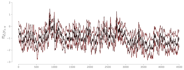
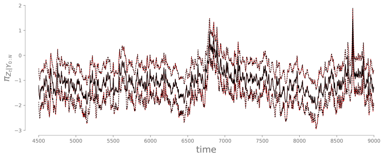
Figure 17: Same as Figure 16, but for a longer assimilation window, i.e., $\pi_{\bm{Z}_{k}|\bm{\theta}^{*},\bm{y}_{0:9000}}$. The smoothing approximation remains excellent despite the widening inference horizon.

Another important note: the sequential approximation of the individual maps $(\mathfrak{M}_{i})$ might present additional challenges due to the accumulation of error, since the target density for the $k$-th map $\mathfrak{M}_{k}$ depends on the numerical approximation of the previous map, $\mathfrak{M}_{k-1}$. This is not an issue with the factorization of $\mathfrak{T}_{k}$ per se, but rather with sequentially computing each element of the factorization. The analysis of sequential Monte Carlo methods (e.g., [18, 25, 107]) addresses a similar accumulation of error, but has not yet been extended to sequential variational inference techniques. In Section 8, we empirically investigate the stability of variational transport map approximations for a problem of very long time smoothing (see Figure 17), showing excellent results—at least for the reconstruction of low-order smoothing marginals.

As shown in (3.9), the computation of each $\mathfrak{M}_{i}$ is also associated with an approximation of the normalizing constant $\mathfrak{c}_{i}$ of its own target density, which then leads to a one-pass approximation of the marginal likelihood using (7.5).

One last remark: the proof of Theorem 7.1 shows that the triangular structure hypothesis for each $\mathfrak{M}_{i}$ can be relaxed provided that the underlying densities are regular enough. The following corollary clarifies this point.

Corollary 7.1.

The results of Theorem 7.1 still hold if we replace every KR rearrangement $\mathfrak{M}_{i}$ with a “block triangular” diffeomorphism of the form (7.2) that couples the same distributions, provided that such regular transport maps exist.

Filtering and smoothing are of course very rich problems, and in this section we have by no means attempted to be exhaustive. Rather, our goal was to highlight some implications of decomposable transports on problems of sequential Bayesian inference, in a general non-Gaussian setting.

7.2 The linear Gaussian case: connection with the RTS smoother

In this section, we specialize the results of Theorem 7.1 to linear Gaussian state-space models, and make explicit the connection with the RTS Gaussian smoother [90].

Consider a linear Gaussian state-space model defined by

$$\bm{Z}_{k+1} = \bm{F}_{k}\,\bm{Z}_{k}+\bm{\varepsilon}_{k}$$ (7.9)

$$\bm{Y}_{k} = \bm{H}_{k}\,\bm{Z}_{k}+\bm{\xi}_{k}$$

for all $k\geq 0$, where $\bm{\varepsilon}_{k}\sim\mathcal{N}(0,\bm{Q}_{k})$, $\bm{\xi}_{k}\sim\mathcal{N}(0,\bm{R}_{k})$, $\bm{F}_{k}\in\mathbb{R}^{n\times n}$, $\bm{H}_{k}\in\mathbb{R}^{d\times n}$, and $\bm{Z}_{0}\sim\mathcal{N}(\mu_{0},\bm{\Gamma}_{0})$. Both $\bm{\varepsilon}_{k}$ and $\bm{\xi}_{k}$ are independent of $\bm{Z}_{k}$, while $\bm{Q}_{k},\bm{R}_{k}$, and $\bm{\Gamma}_{0}$ are symmetric positive definite matrices for all $k\geq 0$.

If we choose an independent reference process $(\bm{X}_{k})$ with standard normal marginals, i.e., $\eta_{\bm{X}_{k}}=\mathcal{N}(0,{\bf I})$, then the maps $(\mathfrak{M}_{k})$ of Theorem 7.1 can be chosen to be linear:

$$\mathfrak{M}_{k}(\bm{z}_{k},\bm{z}_{k+1})=\left[\begin{array}[]{rr}\bm{A}_{k}&\bm{B}_{k}\\ {\bf 0}&\bm{C}_{k}\end{array}\right]\left\{\begin{array}[]{l}\bm{z}_{k}\\ \bm{z}_{k+1}\end{array}\right\}+\left\{\begin{array}[]{l}\bm{a}_{k}\\ \bm{c}_{k}\end{array}\right\},$$ (7.10)

for some matrices $\bm{A}_{k},\bm{B}_{k},\bm{C}_{k}\in\mathbb{R}^{n\times n}$ and $\bm{a}_{k},\bm{c}_{k}\in\mathbb{R}^{n}$. (Notice that in this case Corollary 7.1 applies and the matrices $\bm{A}_{k},\bm{B}_{k}$ can be full and not necessarily triangular.) The following lemma gives a closed form expression for the maps $(\mathfrak{M}_{k})$ with $k\geq 1$. ($\mathfrak{M}_{0}$ can be derived analogously with simple algebra.)

Lemma 7.1 (The linear Gaussian case).

For $k\geq 1$, the map $\mathfrak{M}_{k}$ in (7.10) can be defined as follows: if $(\bm{c}_{k},\bm{C}_{k})$ is the output of a square-root Kalman filter at time $k$ [6], i.e., if $\bm{c}_{k}$ and $\bm{C}_{k}$ are, respectively, the mean and square root of the covariance of the filtering distribution $\pi_{\bm{Z}_{k+1}|\bm{y}_{0:k+1}}$, then one can set:

$$\bm{A}_{k} = \bm{J}_{k}^{-1/2}$$ (7.11)

$$\bm{B}_{k} = -\bm{J}_{k}^{-1}\,\bm{P}_{k}\,\bm{C}_{k}$$

$$\bm{a}_{k} = \bm{J}_{k}^{-1}\,\bm{P}_{k}\,(\bm{F}_{k}\,\bm{c}_{k-1}-\bm{c}_{k}),$$

for $\bm{J}_{k}\coloneqq{\bf I}+\bm{C}_{k-1}^{\top}\,\bm{F}_{k}^{\top}\,\bm{Q}_{k}^{-1}\,\bm{F}_{k}\,\bm{C}_{k-1}$ and $\bm{P}_{k}=-\bm{C}_{k-1}^{\top}\,\bm{F}_{k}^{\top}\,\bm{Q}_{k}^{-1}$.

The formulas in Lemma 7.1 can be interpreted as one possible implementation of a square-root RTS smoother for Gaussian models: at each step $k$ of a forward pass, the filtering estimates $(\bm{c}_{k},\bm{C}_{k})$ are augmented with a collection $(\bm{a}_{k},\bm{A}_{k},\bm{B}_{k})$ of stored quantities, which can then be reused to sample the full Bayesian solution (or particular smoothing marginals) whenever needed, and without ever touching the state-space model again. In this sense, the algorithm proposed in Section 7.1 can be understood as the natural generalization—to the non-Gaussian case—of the square-root RTS smoother.

7.3 Sequential joint parameter and state estimation

In defining a state-space model, it is common to parameterize the transition densities of the unobserved process or the likelihoods of the observables in terms of some hyperparameters $\bm{\Theta}$. The Markov structure of the resulting Bayesian hierarchical model, conditioned on the data, is shown in Figure 8. The state-space model is now fully specified in terms of the conditional densities $(\pi_{\bm{Y}_{k}|\bm{Z}_{k},\bm{\Theta}})_{k\geq 0}$, $(\pi_{\bm{Z}_{k+1}|\bm{Z}_{k},\bm{\Theta}})_{k\geq 0}$, $\pi_{\bm{Z}_{0}|\bm{\Theta}}$, and the marginal $\pi_{\bm{\Theta}}$. We assume that the hyperparameters $\bm{\Theta}$ take values on $\mathbb{R}^{p}$, and that the following regularity conditions hold: $\pi_{\bm{\Theta},\bm{Z}_{0:k-1},\bm{Y}_{0:k-1}}>0$ for all $k\geq 1$.

Given such a parameterization, one often wishes to jointly infer the hidden states and the hyperparameters of the model as observations of the process $(\bm{Y}_{k})$ become available. That is, the goal of inference is to characterize, via a recursive algorithm, the sequence of posterior distributions given by

$$\pi_{\bm{\Theta},\bm{Z}_{0:k}|\bm{y}_{0:k}}(\bm{z}_{\theta},\bm{z}_{0:k})\coloneqq\pi_{\bm{\Theta},\bm{Z}_{0:k}|\bm{Y}_{0:k}}(\bm{z}_{\theta},\bm{z}_{0:k}|\bm{y}_{0:k})$$ (7.12)

for all $k\geq 0$ and for a sequence $(\bm{y}_{k})_{k\geq 0}$ of observations. The following theorem shows that we can characterize (7.12) by computing a sequence of low-dimensional transport maps in the same spirit as Theorem 7.1. In what follows, let $(\bm{X}_{k})$ be an independent process with marginals $(\eta_{\bm{X}_{k}})$ as defined in Theorem 7.1 and let $\bm{X}_{\bm{\Theta}}$ be a random variable on $\mathbb{R}^{p}$ that is independent of $(\bm{X}_{k})$ and with nonvanishing density $\eta_{\bm{X}_{\bm{\Theta}}}$.

(a)

Figure 8: I-map for $\pi_{\bm{\Theta},\bm{Z}_{0},\ldots,\bm{Z}_{N}|\bm{y}_{0},\ldots,\bm{y}_{N}}$, for any $N>0$.

Theorem 7.2 (Decomposition theorem for joint parameter and state estimation).

Let $(\mathfrak{M}_{i})_{i\geq 0}$ be a sequence of $(\sigma_{i})$-generalized KR rearrangements on $\mathbb{R}^{p}\times\mathbb{R}^{n}\times\mathbb{R}^{n}$, which are of the form

$$\mathfrak{M}_{i}(\bm{x}_{\theta},\bm{x}_{i},\bm{x}_{i+1})=\left[\begin{array}[]{l}\mathfrak{M}_{i}^{\bm{\Theta}}(\bm{x}_{\theta})\\[2.0pt] \mathfrak{M}_{i}^{0}(\bm{x}_{\theta},\bm{x}_{i},\bm{x}_{i+1})\\[2.0pt] \mathfrak{M}_{i}^{1}(\bm{x}_{\theta},\bm{x}_{i+1})\end{array}\right]$$ (7.13)

for some $\sigma_{i}$, $\mathfrak{M}_{i}^{\bm{\Theta}}:\mathbb{R}^{p}\rightarrow\mathbb{R}^{p}$, $\mathfrak{M}_{i}^{0}:\mathbb{R}^{p}\times\mathbb{R}^{n}\times\mathbb{R}^{n}\rightarrow\mathbb{R}^{n}$, $\mathfrak{M}_{i}^{1}:\mathbb{R}^{p}\times\mathbb{R}^{n}\rightarrow\mathbb{R}^{n}$, and that are defined by the recursion:

• $\mathfrak{M}_{0}$ pushes forward $\eta_{\bm{X}_{\bm{\Theta}},\bm{X}_{0},\bm{X}_{1}}$ to

  $$\pi^{0}=\widetilde{\pi}^{0}/\mathfrak{c}_{0},$$ (7.14)

• $\mathfrak{M}_{i}$ pushes forward $\eta_{\bm{X}_{\bm{\Theta}},\bm{X}_{i},\bm{X}_{i+1}}$ to

  $$\pi^{i}(\bm{z}_{\theta},\bm{z}_{i},\bm{z}_{i+1})=\eta_{\bm{X}_{\bm{\Theta}},\bm{X}_{i}}(\bm{z}_{\theta},\bm{z}_{i})\,\widetilde{\pi}^{i}(\mathfrak{T}^{\bm{\Theta}}_{i-1}(\bm{z}_{\theta}),\,\mathfrak{M}_{i-1}^{1}(\bm{z}_{\theta},\bm{z}_{i}),\bm{z}_{i+1})/\mathfrak{c}_{i},$$ (7.15)

where $\mathfrak{c}_{i}$ is a normalizing constant, the map $\mathfrak{T}^{\bm{\Theta}}_{j}\coloneqq\mathfrak{M}_{0}^{\bm{\Theta}}\circ\cdots\circ\mathfrak{M}_{j}^{\bm{\Theta}}$ for all $j\geq 0$, and where $(\widetilde{\pi}^{i})_{i\geq 0}$ are functions on $\mathbb{R}^{p}\times\mathbb{R}^{n}\times\mathbb{R}^{n}$ given by:

• $\widetilde{\pi}^{0}(\bm{z}_{\theta},\bm{z}_{0},\bm{z}_{1})=\pi_{\bm{\Theta},\bm{Z}_{0},\bm{Z}_{1}}(\bm{z}_{\theta},\bm{z}_{0},\bm{z}_{1})\,\pi_{\bm{Y}_{0}|\bm{Z}_{0},\bm{\Theta}}(\bm{y}_{0}|\bm{z}_{0},\bm{z}_{\theta})\,\pi_{\bm{Y}_{1}|\bm{Z}_{1},\bm{\Theta}}(\bm{y}_{1}|\bm{z}_{1},\bm{z}_{\theta})$,

• $\widetilde{\pi}^{i}(\bm{z}_{\theta},\bm{z}_{i},\bm{z}_{i+1})=\pi_{\bm{Z}_{i+1}|\bm{Z}_{i},\bm{\Theta}}(\bm{z}_{i+1}|\bm{z}_{i},\bm{z}_{\theta})\,\pi_{\bm{Y}_{i+1}|\bm{Z}_{i+1},\bm{\Theta}}(\bm{y}_{i+1}|\bm{z}_{i+1},\bm{z}_{\theta})$ for $i\geq 1$.

Then, for all $k\geq 0$, the following hold:

1. The map $\widetilde{\mathfrak{M}}_{k}$, defined as

   $$\widetilde{\mathfrak{M}}_{k}(\bm{x}_{\theta},\bm{x}_{k+1})=\left[\begin{array}[]{l}\mathfrak{T}^{\bm{\Theta}}_{k}(\bm{x}_{\theta})\\[2.0pt] \mathfrak{M}_{k}^{1}(\bm{x}_{\theta},\bm{x}_{k+1})\end{array}\right],$$ (7.16)

   pushes forward $\eta_{\bm{X}_{\bm{\Theta}},\bm{X}_{k+1}}$ to $\pi_{\bm{\Theta},\bm{Z}_{k+1}|\bm{y}_{0},\ldots,\bm{y}_{k+1}}$. [filtering]

2. The composition of transport maps $\mathfrak{T}_{k}=T_{0}\circ\cdots\circ T_{k}$, where each $T_{i}$ is defined as

   $$T_{i}(\bm{x}_{\theta},\bm{x}_{0},\ldots,\bm{x}_{k+1})=\left[\begin{array}[]{l}\mathfrak{M}_{i}^{\bm{\Theta}}(\bm{x}_{\theta})\\ \bm{x}_{0}\\ \vdots\\ \bm{x}_{i-1}\\[2.0pt] \mathfrak{M}_{i}^{0}(\bm{x}_{\theta},\bm{x}_{i},\bm{x}_{i+1})\\[2.0pt] \mathfrak{M}_{i}^{1}(\bm{x}_{\theta},\bm{x}_{i+1})\\ \bm{x}_{i+2}\\ \vdots\\ \bm{x}_{k+1}\end{array}\right],$$ (7.17)

   pushes forward $\eta_{\bm{X}_{\bm{\Theta}},\bm{X}_{0},\ldots,\bm{X}_{k+1}}$ to $\pi_{\bm{\Theta},\bm{Z}_{0},\ldots,\bm{Z}_{k+1}|\bm{y}_{0},\ldots,\bm{y}_{k+1}}$. [full Bayesian solution]

3. The model evidence (marginal likelihood) is given by (7.5).

Theorem 7.2 suggests a variational algorithm for the joint parameter and state estimation problem that is similar to the one proposed in Theorem 7.1: compute the sequence of maps $(\mathfrak{M}_{i})$, each of dimension $2n+p$; embed them into higher-dimensional identity maps to form $(T_{i})$ according to (7.17); then evaluate the composition $\mathfrak{T}_{k}=T_{0}\circ\cdots\circ T_{k}$ to sample directly from $\pi_{\bm{\Theta},\bm{Z}_{0:k+1}|\bm{y}_{0:k+1}}$ (i.e., the full Bayesian solution). See Appendix C for more details. Each map $\mathfrak{M}_{i}$ is now of dimension twice that of the model state plus the dimension of the hyperparameters. This dimension is slightly higher than that of the maps $(\mathfrak{M}_{i})$ considered in Theorem 7.1, and should be regarded as the price to pay for introducing hyperparameters in the state-space model and having to deal with the Markov structure of Figure 8 as opposed to the tree structure of Figure 7. By Theorem 7.2[Part 1], the composition of maps $\mathfrak{T}^{\bm{\Theta}}_{k}=\mathfrak{M}_{0}^{\bm{\Theta}}\circ\cdots\circ\mathfrak{M}_{k}^{\bm{\Theta}}$ provides a recursive characterization of the posterior distribution over the static parameters, $\pi_{\bm{\Theta}|\bm{y}_{0:k+1}}$, for all $k\geq 0$. The latter is often the ultimate goal of inference [2]. In order to have a sequential algorithm for parameter estimation, we also need to keep a running approximation of $\mathfrak{T}^{\bm{\Theta}}_{k}$ using the recursion $\mathfrak{T}^{\bm{\Theta}}_{k}=\mathfrak{T}^{\bm{\Theta}}_{k-1}\circ\mathfrak{M}_{k}^{\bm{\Theta}}$—e.g., via regression—so that the cost of evaluating $\mathfrak{T}^{\bm{\Theta}}_{k}$ does not grow with $k$.

Even in the joint parameter and state estimation case, only a single forward pass with local computations is necessary to gather all the information from the state-space model needed to sample the collection of posteriors $(\pi_{\bm{\Theta},\,\bm{Z}_{0:k+1}|\bm{y}_{0:k+1}})$. Notice that the accuracy of the variational procedure is only limited by the accuracy of each computed map, and that the proposed approach does not prescribe an artificial dynamic for the parameters [60, 68], or an a priori fixed-lag smoothing approximation [86]. Yet there is no rigorous proof that the performance of the proposed sequential algorithm for parameter estimation does not deteriorate with time. Indeed, developing exact, sequential, and online algorithms for parameter estimation in general non-Gaussian state-space models is among the chief research challenges in SMC methods [52]. See [15, 19, 26] for recent contributions in this direction and [55] for a review of SMC approaches to Bayesian parameter inference. See also [34] for a hybrid approach that combines elements of variational inference with particle filters.

We refer the reader to Section 8 for a numerical illustration of parameter inference with transport maps involving a stochastic volatility model.

7.4 Fixed-point smoothing

Consider again the problem of sequential inference in a state-space model without static parameters (see Figure 7), and suppose that we are interested only in the smoothing marginal $\pi_{\bm{Z}_{0}|\bm{y}_{0:k}}$ for all $k\geq 0$; this is the fixed-point smoothing problem [104].

In Section 7.1 we showed that computing a sequence of maps $(\mathfrak{M}_{i})$—each of dimension $2n$—is sufficient to sample the joint distribution $\pi_{\bm{Z}_{0:k+1}|\bm{y}_{0:k+1}}$ by evaluating the composition $\mathfrak{T}_{k}=T_{0}\circ\cdots\circ T_{k}$, where each $T_{i}$ is a trivial embedding of $\mathfrak{M}_{i}$ into an identity map. If we can sample $\pi_{\bm{Z}_{0:k+1}|\bm{y}_{0:k+1}}$, then it is easy to obtain samples from the marginal $\pi_{\bm{Z}_{0}|\bm{y}_{0:k+1}}$: in fact, it suffices to evaluate only the first $n$ components of $\mathfrak{T}_{k}$, which can be interpreted as a map from $\mathbb{R}^{n\times(k+2)}$ to $\mathbb{R}^{n}$. To do so, however, we need to evaluate $k$ maps. A natural question then is whether it is possible to characterize $\pi_{\bm{Z}_{0}|\bm{y}_{0:k+1}}$ via a single transport map that is updated recursively in time, as opposed to a growing composition of maps.

Here we propose a solution—certainly not the only possibility—based on the theory of Section 7.3. The idea is to treat $\bm{Z}_{0}$ as a static parameter, i.e., to set $\bm{\Theta}\coloneqq\bm{Z}_{0}$ and apply the results of Theorem 7.2 to the Markov structure of Figure 9. The resulting algorithm computes a sequence of maps $(\mathfrak{M}_{i})$ of dimension $3n$, i.e., three times the state dimension, and keeps a running approximation of $\mathfrak{T}^{\bm{\Theta}}_{k}$ via the recursion $\mathfrak{T}^{\bm{\Theta}}_{k}=\mathfrak{T}^{\bm{\Theta}}_{k-1}\circ\mathfrak{M}_{k}^{\bm{\Theta}}$, where each $\mathfrak{M}_{k}^{\bm{\Theta}}$ is just a subcomponent of $\mathfrak{M}_{k}$. These maps $(\mathfrak{M}_{i})$ are higher-dimensional than those considered in Section 7.1, but they do yield the desired result: each $\mathfrak{T}^{\bm{\Theta}}_{k}:\mathbb{R}^{n}\rightarrow\mathbb{R}^{n}$ characterizes the smoothing marginal $\pi_{\bm{Z}_{0}|\bm{y}_{0:k+1}}$, for all $k\geq 0$, via a single transport map that is updated recursively in time with just one forward pass (see Theorem 7.2[Part 1]).

(a)

Figure 9: I-map (certainly not minimal) for $\pi_{\bm{Z}_{0},\bm{Z}_{1:N}|\bm{y}_{0:N}}$, for any $N>0$. Orange edges have been added compared to the tree structure of Figure 7.

8 Numerical illustration

We illustrate some aspects of the preceding theory using a problem of sequential inference in a non-Gaussian state-space model. In particular, we show the application of decomposable transport maps (Sections 6 and 7) to joint state and parameter inference in a stochastic volatility model. This example is intended as a direct and simple illustration of the theory. The notion of decomposable transport maps is useful well beyond the sequential inference setting, and entails the general problem of inference in continuous non-Gaussian graphical models. We refer the reader to [78] for an application of the theory of sparse transports (Section 5) to the problem of learning the Markov structure of a non-Gaussian distribution, and we defer further numerical investigations to a dedicated paper [7].

Following [57, 100], we model the scalar log-volatility $(\bm{Z}_{k})$ of the return of a financial asset at time $k=0,\ldots,N$ using an autoregressive process of order one, which is fully specified by $\bm{Z}_{k+1}=\bm{\mu}+\bm{\phi}\,(\bm{Z}_{k}-\bm{\mu})+\,\bm{\varepsilon}_{k}$, for all $k\geq 0$, where $\bm{\varepsilon}_{k}\sim\mathcal{N}(0,1/16)$ is independent of $\bm{Z}_{k}$, $\bm{Z}_{0}|\bm{\mu},\bm{\phi}\sim\mathcal{N}(\bm{\mu},\frac{1}{1-\bm{\phi}^{2}})$, and where $\bm{\phi}$ and $\bm{\mu}$ represent scalar hyperparameters of the model. In particular, $\bm{\mu}\sim\mathcal{N}(0,1)$ and $\bm{\phi}=2\exp(\bm{\phi}^{\star})/(1+\exp(\bm{\phi}^{\star}))-1$ with $\bm{\phi}^{\star}\sim\mathcal{N}(3,1)$. We define $\bm{\Theta}\coloneqq(\bm{\mu},\bm{\phi})$. The process $(\bm{Z}_{k})$ and parameters $\bm{\Theta}$ are unobserved and must be estimated from an observed process $(\bm{Y}_{k})$, which represents the mean return on holding the asset at time $k$, $\bm{Y}_{k}=\bm{\xi}_{k}\,\exp(\frac{1}{2}\bm{Z}_{k})$, where $\bm{\xi}_{k}$ is a standard normal random variable independent of $\bm{Z}_{k}$. As a dataset $(\bm{y}_{k})_{k=0}^{N}$, we use the $N+1$ daily differences of the pound/dollar exchange rate starting on 1 October 1981, with $N=944$ [100, 33].

Our goal is to sequentially characterize $\pi_{\bm{\Theta},\bm{Z}_{0:k}|\bm{y}_{0:k}}$, for all $k=0,\ldots,N$, as observations $(\bm{y}_{k})$ become available. The Markov structure of $\pi_{\bm{\Theta},\bm{Z}_{0:N}|\bm{y}_{0:N}}$ matches Figure 8. We solve the problem using the algorithm introduced in Section 7.3: we compute a sequence, $(\mathfrak{M}_{j})_{j=0}^{N-1}$, of four-dimensional transport maps ($n=\text{dim}(\bm{Z}_{j})=1$ and $p=\text{dim}(\bm{\Theta})=2$) according to their definition in Theorem 7.2 and using the variational form (3). All reference densities are standard Gaussians. Then, by Theorem 7.2[part 1], for any $k<N$, we can easily sample the filtering marginal $\pi_{\bm{Z}_{k+1}|\bm{y}_{0:k+1}}$ by pushing forward a standard normal through the subcomponent $\mathfrak{M}_{k}^{1}$ of $\mathfrak{M}_{k}$, and we can also sample the posterior distribution over the static parameters $\pi_{\bm{\Theta}|\bm{y}_{0:k+1}}$ by pushing forward a standard normal through the map $\mathfrak{T}^{\bm{\Theta}}_{k}$. The map $\mathfrak{T}^{\bm{\Theta}}_{k}=\mathfrak{M}_{0}^{\bm{\Theta}}\circ\cdots\circ\mathfrak{M}_{k}^{\bm{\Theta}}$ is updated sequentially over time (via regression) using the recursion $\mathfrak{T}^{\bm{\Theta}}_{k}=\mathfrak{T}^{\bm{\Theta}}_{k-1}\circ\mathfrak{M}_{k}^{\bm{\Theta}}$, so that the cost of evaluating $\mathfrak{T}^{\bm{\Theta}}_{k}$ does not increase with $k$. The resulting algorithm for parameter estimation is thus sequential. Moreover, if we want to sample $\pi_{\bm{\Theta},\bm{Z}_{0:k+1}|\bm{Y}_{0:k+1}}$—the full Bayesian solution at time $k+1$—we simply need to embed each $\mathfrak{M}_{j}$ into an identity map to form the transport $T_{j}$, for $j=0,\ldots,k$, and push forward reference samples through the composition $\mathfrak{T}_{k}=T_{0}\circ\cdots\circ T_{k}$ (Theorem 7.2[part 2]). See Appendix C for pseudocode of the relevant algorithms.

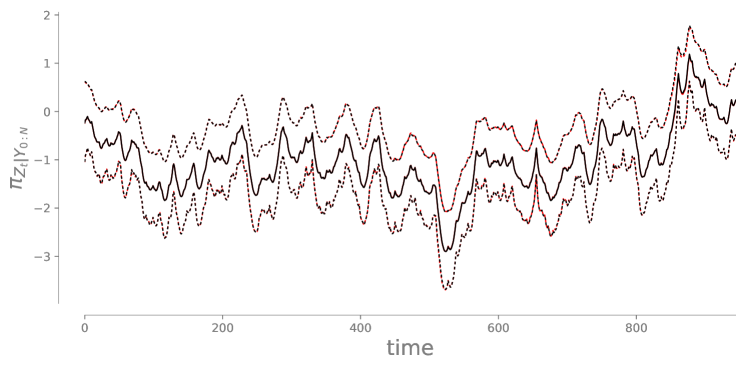
Figure 10: Comparison between the $\{5,95\}$–percentiles (dashed lines) and the mean (solid line) of the numerical approximation of the smoothing marginals $\pi_{\bm{Z}_{k}|\bm{y}_{0:N}}$ via transport maps (red lines) versus a “reference” MCMC solution (black lines), for $k=0,\ldots,N$. The two solutions are indistinguishable.

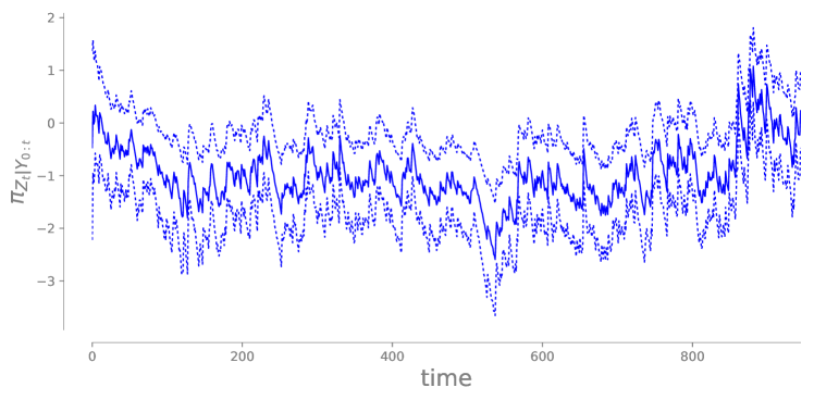
Figure 11: At each time $k$, we illustrate the $\{5,95\}$–percentiles (dotted lines) and the mean (solid line) of the numerical approximation of the filtering distribution $\pi_{\bm{Z}_{k}|\bm{y}_{0:k}}$, for $k=0,\ldots,N$.

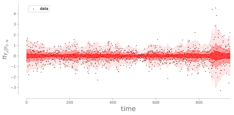
Figure 14: Shaded regions represent the $\{5,25,40,60,75,95\}$–percentiles of the marginals of the posterior predictive distribution (conditioning on all the data), along with black dots that represent the observed data $(\bm{y}_{k})_{k=0}^{N}$.

Figures 11 and 10 show the resulting filtering and smoothing marginals of the states over time, respectively. Figures 12 and 13 collect the corresponding posterior marginals of the static parameters over time. Figure 14 illustrates marginals of the posterior predictive distribution of the data, together with the observed data $(\bm{y}_{k})$, showing excellent coverage overall.

Our results rely on a numerical approximation of the desired transport maps. Each component of $\mathfrak{M}_{k}$ is parameterized via the monotone representation (3.4), with $(a_{k})$ and $(b_{k})$ chosen to be Hermite polynomials and functions, respectively, of total degree seven [12] . The expectation in (3) is approximated using tensorized Gauss quadrature rules. The resulting minimization problems are solved sequentially using the Newton-CG method [120]. This test case was run using the dedicated software package publicly available at http://transportmaps.mit.edu. The website contains details about additional possible parameterizations of the maps.

There are several ways to investigate the quality of these approximations. Figures 10, 12, and 13 compare the numerical approximation (via a decomposable transport map) of the smoothing marginals of the states and the posteriors of the static parameters to a “reference” solution obtained via MCMC. The MCMC chain is run until it yields $10^{5}$ effectively independent samples. The two solutions agree remarkably well and are almost indistinguishable in most places. (Of course, MCMC in this context is not a data-sequential algorithm; it requires that all the data $(\bm{y}_{k})_{k=0}^{N}$ be available simultaneously.) An important fact is that the MCMC chain is generated using an independent proposal [96] given by the pushforward of a standard Gaussian through the numerical approximation of $\mathfrak{T}_{N-1}$ (denoted as $\widetilde{\mathfrak{T}}_{N-1}$). The resulting MCMC chain has an acceptance rate slightly above $75\%$, confirming the overall quality of the variational approximation. We notice, however, a slow accumulation of error in the posterior marginal for the static parameter $\bm{\mu}$ (Figure 13). This is not surprising since we are performing sequential parameter inference [52].

A second quality test can proceed as follows: since we use a standard Gaussian reference distribution $\bm{\nu}_{\eta}$, we expect the pullback of $\pi_{\bm{\Theta},\bm{Z}_{0:N}|\bm{y}_{0:N}}$ through $\widetilde{\mathfrak{T}}_{N-1}$ to be close to a standard Gaussian. Figure 15 supports this claim by showing a collection of random two-dimensional conditionals of the approximate pullback: these “slices” of the 947-dimensional ($N$+1 states plus two hyperparameters) pullback distribution are identical to a two-dimensional standard normal, as expected. The fact that we can evaluate the approximate pullback density is one of the key features of this variational approach to inference. Even more, we can use this approximate pullback density to estimate the KL divergence between our target $\bm{\nu}_{\pi}$ (the full Bayesian solution at time $N$) and the approximating measure $(\widetilde{\mathfrak{T}}_{N-1})_{\sharp}\bm{\nu}_{\eta}$, via the variance diagnostic in (3.8). A numerical realization of (3.8) yields $\mathcal{D}_{\rm KL}(\,(\widetilde{\mathfrak{T}}_{N-1})_{\sharp}\bm{\nu}_{\eta}\,||\,\bm{\nu}_{\pi}\,)\approx 1.07\times 10^{-1}$, which confirms the good numerical approximation of $\bm{\nu}_{\pi}$, a 947-dimensional target measure. For comparison, we note that the KL divergence from $\bm{\nu}_{\pi}$ to its Laplace approximation (a Gaussian approximation at the mode) is $\approx 5.68$—considerably worse than what is achieved through optimization of a nonlinear transport map. Moreover, the Laplace approximation cannot be computed sequentially with a constant effort per time step.

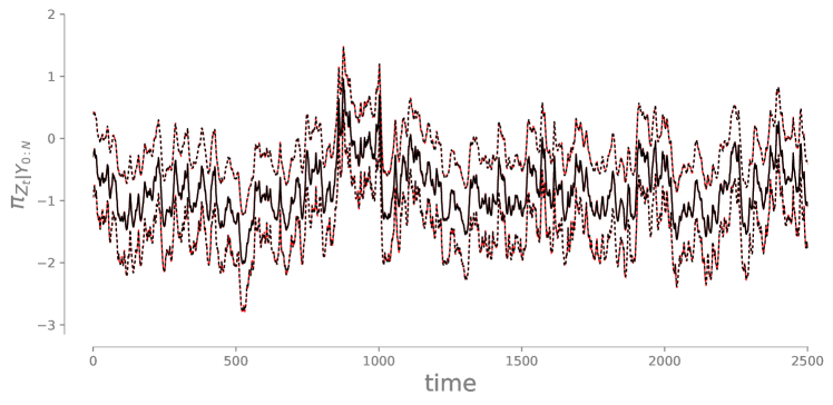
Figure 16: Comparison between the $\{5,95\}$–percentiles (dashed lines) and the mean (solid line) of the transport map numerical approximation of the smoothing marginals $\pi_{\bm{Z}_{k}|\bm{\theta}^{*},\bm{y}_{0:2500}}$, with $\bm{\theta}^{*}={\rm med}[\Theta|\bm{y}_{0},\ldots,\bm{y}_{N}]$ (red lines), and a reference MCMC solution (black lines). The two solutions are indistinguishable.

While a slow accumulation of errors is expected for sequential parameter inference, we also wish to investigate the stability of our transport map approximation for recursive smoothing without static parameters. We try the following experiment: (1) compute the posterior medians of the static parameters after $N+1=945$ days, i.e., $\bm{\theta}^{*}={\rm med}[\Theta|\bm{y}_{0},\ldots,\bm{y}_{944}]$; and then (2) use these parameters to characterize the smoothing distribution $\pi_{\bm{Z}_{0},\ldots,\bm{Z}_{2500}|\bm{\theta}^{\ast},\,\bm{y}_{0},\ldots,\,\bm{y}_{2500}}$ of the log-volatility over (roughly) the next ten years worth of exchanges, using the sequential algorithm proposed in Section 7.1, which in this case amounts to computing only a sequence of two-dimensional maps $(\mathfrak{M}_{k})$. The resulting smoothing marginals are shown in Figure 16 and compared to those of a reference MCMC simulation with $10^{5}$ effectively independent samples; we observe excellent agreement despite the long assimilation window. We then repeat the same experiment for an even longer assimilation window, i.e., 9009 steps or roughly 35 years. Figure 17 shows the remarkable stability of the resulting smoothing approximation, at least for low-order marginals. In fact, even the approximation of the joint distribution of the states is quite good, as reported in the last column of Table 1. Understanding how errors propagate in this variational framework—and what could be potential mechanisms for the “dissipation” of errors—is an exciting avenue for future work.

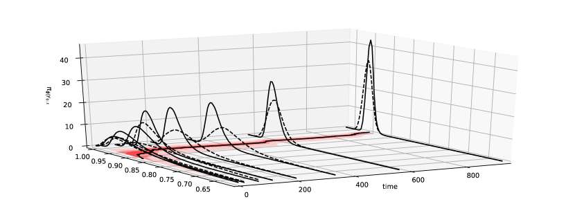
Figure 20: Same as Figure 12, but using linear maps. Here, the loss of accuracy is more dramatic than for the smoothing distribution of the state in Figure 18. Even though the approximate marginal captures the bulk of the true parameter marginals, for this specific problem of static parameter inference, a linear map is largely inadequate; hence the need for a higher-order nonlinear transformation.

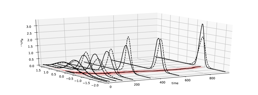
Figure 22: Same as Figure 13, but using linear maps. Once again, the linear map provides plausible, but somewhat inaccurate, results for sequential parameter inference. A nonlinear transformation is better suited for this problem.

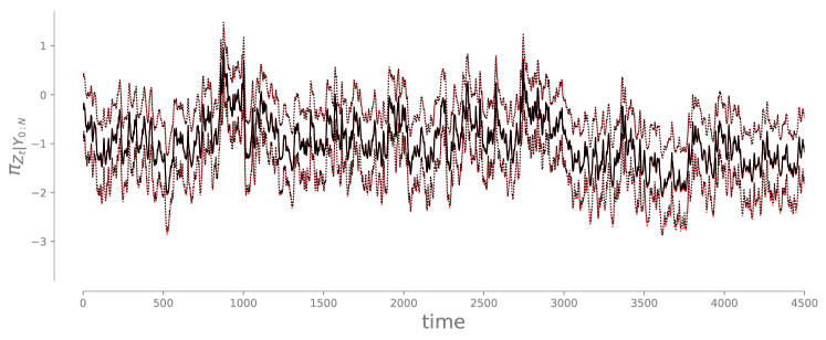
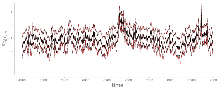
Figure 24: Same as Figure 17, but using linear maps. Long-time smoothing with no static parameters via linear maps yields accurate characterizations of the marginal distributions across all times, at a fraction of the cost of a high-order nonlinear transformation (see Table 1).

The results presented so far are very accurate, but also expensive. Table 1 collects the computational times for the joint state-parameter inference problem (approximately two days) and for the long-time (9009 step) smoothing problem (approximately 40 minutes), using a degree-seven map. While there remains a tremendous opportunity to develop more performance-oriented versions of our transport map code, specialized to the problem of sequential inference, the present framework also offers a practical and powerful tradeoff between computational cost and accuracy. In Appendix D, we re-run all our test cases using linear, rather than degree seven, parameterizations of the maps $\{\mathfrak{M}_{k}\}$. Table 1 shows that the computational times are dramatically reduced: from two days to approximately one minute for the joint state-parameter inference problem, and from 40 minutes to 7 minutes for the long-time smoothing problem. The reduction in computational time comes, of course, at the price of accuracy; see last column of Table 1. This reduction in accuracy may or may not be acceptable. For instance, in Figure 24, it is difficult to distinguish the linear map approximation from the reference MCMC solution. Quantitatively, we know from Table 1 that a linear map is worse at approximating the full Bayesian solution than a degree-7 transformation. Yet, as far as quantiles of low-order marginals are concerned, the two solutions are indistinguishable (Figure 24); in an applied setting, this accuracy may be more than sufficient. In other cases, however, a linear map might be inadequate. For example, the parameter marginals in Figures 20 and 22, estimated using linear maps, are much worse than their degree-7 counterparts (Figures 12 and 13). In these cases, we need nonlinear transformations.

Clearly, there is a rich spectrum of possibilities between a linear and a high-order transport map. Some parameterizations can scale with dimension (e.g., separable but nonlinear representations), while others do not (e.g., total-degree polynomial expansions). Depending on the problem, some parameterizations will lead to accurate results, while others will not. Yet, the cost-accuracy tradeoff in the transport framework can be controlled, e.g., by estimating the quality of a given approximation using (3.8).

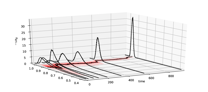
Figure 12: (Horizontal plane) At each time $k$, we illustrate the $\{5,25,40,60,75,95\}$–percentiles (shaded regions) and the mean (solid line) of the numerical approximation of $\pi_{\bm{\phi}|\bm{y}_{0:k}}$, the posterior marginal of the static parameter $\bm{\phi}$. (Vertical axis) At several times $k$ we also compare the transport map numerical approximation of $\pi_{\bm{\phi}|\bm{y}_{0:k}}$ (solid lines) with a reference MCMC solution (dashed lines). The two distributions agree remarkably well.

Type	# steps	Order	Time [m : s]	# cores	Figures	Var. diag. (3.8)
S/P	945	Laplace	00 : 04	1		$5.68$
		7	$\approx$ 2 days	64	10 – 15	$1.07\times 10^{-1}$
		linear	01 : 14	1	18 – 23	$1.77$
S	9009	Laplace	00 : 42	1		$10.0$
		7	42 : 50	1	17	$1.19\times 10^{-1}$
		linear	06 : 40	1	24	$5.01$

Table 1: Computational effort required to compute a decomposable transport map for different complexities of the transformations $\mathfrak{M}_{k}$—linear versus degree seven—and for different inference scenarios—smoothing and static parameter estimation (top row) or long-time smoothing without static parameters (bottom row), for the stochastic volatility model of Section 8. The last column reports the variance diagnostic (3.8) for the corresponding joint posterior, not just a few marginals. It highlights a tradeoff between cost and accuracy, typical of the transport map approach to variational inference. For comparison, we also report the cost and accuracy of a simple Laplace approximation, which requires no formal optimization.

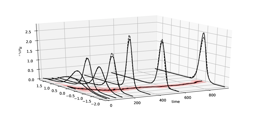
Figure 13: Same as Figure 12, but for the static parameter $\bm{\mu}$.

Figure 15: Randomly chosen two-dimensional conditionals of the pullback of $\pi_{\bm{\Theta},\bm{Z}_{0:N}|\bm{y}_{0:N}}$ through the numerical approximation of $\mathfrak{T}_{N-1}$. Since we use a standard normal reference distribution, the numerical approximation of $\mathfrak{T}_{N-1}$ should be deemed satisfactory if the pullback density is close to a standard normal, as it is here.

9 Discussion

This paper has focused on the problem of coupling a pair $(\bm{\nu}_{\eta},\bm{\nu}_{\pi})$ of absolutely continuous measures on $\mathbb{R}^{n}$, for the purpose of sampling or integration. If $\bm{\nu}_{\eta}$ is a tractable measure (e.g., an isotropic Gaussian) and $\bm{\nu}_{\pi}$ is an intractable measure of interest (e.g., a posterior distribution), then a deterministic coupling enables principled approximations of integrals via the identity $\int g\,{\rm d}\bm{\nu}_{\pi}=\int g\circ T\,{\rm d}\bm{\nu}_{\eta}$. In other words, a deterministic coupling provides a simple way to simulate $\bm{\nu}_{\pi}$ by pushing forward samples from $\bm{\nu}_{\eta}$ through a transport map $T$. This idea, modulo some variations, has been exploited in a variety of statistical and machine learning applications—some old, some new—including random number generation [72], variational inference [80, 105, 95, 69, 73], the computation of model evidence [76], model learning and density estimation [115, 64, 1, 113], non-Gaussian proposals for MCMC or importance sampling [84, 4, 79, 49, 82, 48], multiscale modeling [85], and filtering [22, 16, 93, 92], to name a few. Indeed there are infinitely many ways to transport one measure to another [117] and as many ways to compute one. Yet these maps are not equally easy to characterize.

This paper establishes an explicit link between the conditional independence structure of $(\bm{\nu}_{\eta},\bm{\nu}_{\pi})$ and the existence of low-dimensional couplings induced by transport maps that are sparse and/or decomposable. These results can enhance a wide array of numerical approaches to the transportation of measures, including [91, 80, 115, 95, 69, 7], and thus facilitate simulation with respect to complex distributions in high dimensions. We briefly discuss our main results below.

Sparse transports.

A sparse transport is a map whose components do not depend on all input variables. Section 5 derives tight bounds on the sparsity pattern of the Knothe–Rosenblatt (KR) rearrangement (a triangular transport map) based solely on the Markov structure of $\bm{\nu}_{\pi}$, provided that $\bm{\nu}_{\eta}$ is a product measure (Theorem 5.1). This analysis shows that the inverse of the KR rearrangement is the natural generalization to the non-Gaussian case of the Cholesky factor of the precision matrix of a Gaussian MRF—in that both the inverse KR rearrangement (a potentially nonlinear map) and the Cholesky factor (a linear map) have the same sparsity pattern given target measures with the same Markov structure. Thus the KR rearrangement can be used to extend well-known modeling and sampling techniques for high-dimensional Gaussian MRFs [99] to non-Gaussian fields (Section 5.2). These results are particularly useful when constructing a transport map from samples via convex optimization [83] and suggest novel approaches to model learning [78] and high-dimensional filtering [109, Chapter 6]. Section 5 shows that sparsity is usually a feature of inverse transports, while direct transports tend to be dense, even for the most trivial Markov structures. In fact, the sparsity of direct transports stems from marginal (rather than conditional) independence—a property frequently exploited in localization schemes for high-dimensional covariance estimation [39, 46].

Decomposable transports.

A decomposable map is a function that can be written as the composition of finitely many low-dimensional maps that are triangular up to a permutation—i.e., $T=T_{1}\circ\cdots\circ T_{\ell}$, where each $T_{i}$ differs from the identity only along a small subset of its components and is a generalized triangular function as defined in Section 6. Theorem 6.1 shows that every target measure whose Markov network admits a graph decomposition can be coupled with a product (reference) measure via a decomposable map. Decomposable maps are important because they are much easier to represent than arbitrary multivariate functions on $\mathbb{R}^{n}$. In general, these maps are non-triangular, even though each map in the composition is generalized triangular.

The notion of a decomposable map is different from the composition-of-maps approaches advocated in the literature for the approximation of transport maps (e.g., consider normalizing flows [95] or Stein variational algorithms [1, 69, 27], but also [115, 64]). In these approaches, very simple maps $(M_{i})_{i\geq 1}$ are composed in growing number to define a transport map of increasing complexity, $M=M_{1}\circ\cdots\circ M_{k}$. The number of layers in $M$ depends on the desired accuracy of the transport and can be arbitrarily large. On the other hand, a decomposable coupling is induced by a special transport map that can be written exactly as the composition of finitely many maps, $T=T_{1}\circ\cdots\circ T_{\ell}$, where each $T_{i}$ has a specific sparsity pattern that makes it low-dimensional. This definition does not specify a representation for $T_{i}$. In fact, each $T_{i}$ could itself be approximated by the composition of simple maps using any of the aforementioned techniques. The advantage of targeting a decomposable transport is the fact that the $(T_{i})$ are guaranteed to be low-dimensional.

Approximate Markov properties.

Sparsity and decomposability of certain transport maps are induced by the Markov properties of the target measure. A natural question is: what happens when $\bm{\nu}_{\pi}$ satisfies some Markov properties only approximately? In particular, let $\bm{\nu}_{\pi}$ be Markov with respect to $\bm{\mathcal{G}}$, and assume that there exists a measure $\hat{\bm{\nu}}\in\mathscr{M}_{+}(\mathbb{R}^{n})$ which is Markov with respect to a graph $\hat{\bm{\mathcal{G}}}$ that is sparser than $\bm{\mathcal{G}}$ and such that $\mathcal{D}_{\rm KL}(\,\hat{\bm{\nu}}\,||\,\bm{\nu}_{\pi}\,)<\varepsilon$, for some $\varepsilon>0$. For small $\varepsilon$, we would be tempted to use $\hat{\bm{\mathcal{G}}}$ to characterize couplings of $(\bm{\nu}_{\eta},\bm{\nu}_{\pi})$ that are possibly sparser or more decomposable than those associated with $\bm{\mathcal{G}}$. Concretely, if we are interested in a triangular transport that pushes forward $\bm{\nu}_{\eta}$ to $\bm{\nu}_{\pi}$, we could minimize $\mathcal{D}_{\rm KL}(\,T_{\sharp}\,\bm{\nu}_{\eta}\,||\,\bm{\nu}_{\pi}\,)$ over the set of maps that have the same sparsity pattern as the KR rearrangement between $\bm{\nu}_{\eta}$ and $\hat{\bm{\nu}}$. Bounds on this sparsity pattern are given by Theorem 5.1 using only graph operations on $\hat{\bm{\mathcal{G}}}$; no explicit knowledge of $\hat{\bm{\nu}}$ is required. Alternatively, if we are interested in decomposable transports that push forward $\bm{\nu}_{\eta}$ to $\bm{\nu}_{\pi}$, we could minimize $\mathcal{D}_{\rm KL}(\,T_{\sharp}\,\bm{\nu}_{\eta}\,||\,\bm{\nu}_{\pi}\,)$ over the set of maps that factorize as any of the decomposable transports between $\bm{\nu}_{\eta}$ and $\hat{\bm{\nu}}$. The shapes of these low-dimensional factorizations are given by Theorem 6.1 using, once again, only graph operations on $\hat{\bm{\mathcal{G}}}$.

Now let $\hat{\mathcal{T}}$ denote the set of maps whose structure is constrained by $\hat{\bm{\mathcal{G}}}$ in terms of sparsity or decomposability. It is easy to show that

$$\min_{T\in\hat{\mathcal{T}}}\mathcal{D}_{\rm KL}(\,T_{\sharp}\,\bm{\nu}_{\eta}\,||\,\bm{\nu}_{\pi}\,)<\varepsilon,$$ (9.1)

which means that the price of assuming that the coupling is either sparser or more decomposable than it ought to be is just a small error in the approximation of $\bm{\nu}_{\pi}$.

Of course, the pending question is whether $\bm{\nu}_{\pi}$ can be well approximated by a measure that satisfies additional Markov properties. There is some work on this topic, e.g., [54, 53, 14]—especially in the case of Gaussian measures—but a more thorough investigation of the problem remains an open and important direction for future work. Interestingly, the transport map framework also allows one to adaptively discover information about low-dimensional couplings. For instance, one might start with a very sparse transport map and then incrementally decrease the sparsity level of the map until the resulting approximation of $\bm{\nu}_{\pi}$ becomes satisfactory. The same can be done for decomposable transports. See [7] for some details on this idea.

Filtering and smoothing.

Section 6.4 shows how not only the representation, but also the computation, of a decomposable map, $T=T_{1}\circ\cdots\circ T_{\ell}$, can be broken into a sequence of $\ell$ simpler steps, each associated with a low-dimensional optimization problem whose solution yields $T_{i}$. We give a concrete example of this idea for filtering, smoothing, and joint state–parameter inference in nonlinear and non-Gaussian state-space models (Section 7). In this context, Theorems 7.1 and 7.2 introduce variational approaches for characterizing the full posterior distribution of the sequential inference problem, essentially by performing only recursive lag–1 smoothing with transport maps. The proposed approaches consist of a single forward pass on the state-space model, and generalize the square-root Rauch-Tung-Striebel smoother to non-Gaussian models (see Section 7.2). In practice, we should think of Theorems 7.1 and 7.2 as providing “meta-algorithms” within which all kinds of approximations can be introduced, e.g., linearizations of the forward model, restriction to linear maps, and approximate flows [22, 69], to name a few. These approximations are the workhorse of modern approaches to large-scale filtering, e.g., data assimilation in geophysical applications [104, 36], and may play a key role in further instantiations of the “meta-algorithms” proposed in Section 7. Of course, it would be desirable to complement such variational approximations with a rigorous error analysis, analogous to the analysis available for SMC methods (e.g., [18, 25, 107]). It is also important to note that one can always use functionals like (3.8) to estimate the quality of a given approximate map, or use the map itself to build sophisticated proposals for sampling techniques like MCMC [84].

A recent approach that constructs an approximation of the KR rearrangement for sequential inference is the “Gibbs flow” of [49]; here, the authors define a proposal for SMC (or MCMC) methods using the solution map of a discretized ordinary differential equation (ODE) whose drift term depends only on the full conditionals of the target distribution. Evaluating the solution map only requires the evaluation of one-dimensional integrals, and the action of this map implicitly defines a transport, without any explicit parameterization of the transformation. Several other filtering approaches in the literature, e.g., [23, 122], rely on the solution of ODEs that are different from [49], but also inspired by ideas from mass transportation. Implicit sampling for particle filters [16] also implicitly constructs a transport map, from a standard Gaussian to a particular approximation of the filtering distribution; the action of this transport is realized by solving an optimization/root-finding problem for each sample [70].

One of the first efforts to use optimal transport in filtering is [92], which constructs an optimal transport plan between an empirical approximation of the forecast distribution (given by simulating the prior dynamic) and a corresponding empirical approximation of the filtering distribution, obtained by reweighing the forecast ensemble according to the likelihood. Thus, [92] solves a discrete Kantorovich optimal transport problem instead of a continuous problem for a transport map (cf. Section 7.1). A linear transformation of the forecast ensemble is then derived from the optimal plan. In this approach, the explicit construction of couplings is used only to update the forecast distribution, instead of the previous filtering marginal.

Further extensions.

We envision many additional ways to extend the present work. For instance, it would be interesting to investigate the low-dimensional structure of deterministic couplings between pair of measures $(\bm{\nu}_{\eta},\bm{\nu}_{\pi})$ that are not absolutely continuous and that need not be defined on the same space $\mathbb{R}^{n}$. Such couplings are usually induced by “random” maps and can be particularly effective for approximating multi-modal distributions; see the warp bridge transformations in [76, 118] for some examples.

Finally, we emphasize that this paper characterizes some classes of low-dimensional maps, but certainly not all. In particular, low dimensionality need not stem from the Markov properties of the underlying measures. In ongoing work we are exploring the notion of low-rank couplings: these are induced by transport maps that are low-dimensional up to a rotation of the space, i.e., maps whose action is nontrivial only along a low-dimensional subspace. This type of structure appears quite naturally in certain high-dimensional Bayesian inference problems (e.g., inverse problems [114] and spatial statistics) where the data may be informative only about a few linear combinations of the latent parameters [110, 21, 111]. Low-rank structure can be detected via certain average derivative functionals [102, 17] but cannot be deduced, in general, from the Markov structure of $(\bm{\nu}_{\eta},\bm{\nu}_{\pi})$.

Acknowledgments

We would like to thank Ricardo Baptista, Chi Feng, Jeremy Heng, Pierre Jacob, Qiang Liu, Rebecca Morrison, Zheng Wang, Alan Willsky, Olivier Zahm, and Benjamin Zhang for many insightful discussions and for pointing us to key references in the literature. This work was supported in part by the US Department of Energy, Office of Advanced Scientific Computing (ASCR), under grant numbers DE-SC0003908 and DE-SC0009297.

A Generalized Knothe-Rosenblatt rearrangement

In this section we first review the classical notion of KR rearrangement [97, 61], and then give a formal definition for a generalized KR rearrangement, i.e., a transport map that is lower triangular up to a permutation. A disclaimer: these transports can also be defined under weaker conditions than those considered here, at the expense, however, of some useful regularity (e.g., see [10]).

The following definition introduces the one-dimensional version of the KR-rearrangement, and it is key to extend the transport to higher dimensions.

Definition A.1 (Increasing rearrangement on $\mathbb{R}$).

Let $\bm{\nu}_{\eta},\bm{\nu}_{\pi}\in\mathscr{M}_{+}(\mathbb{R})$, and let $F,G$ be their respective cumulative distribution functions, i.e., $F(t)=\bm{\nu}_{\eta}((-\infty,t))$ and $G(t)=\bm{\nu}_{\pi}((-\infty,t))$. Then the increasing rearrangement on $\mathbb{R}$ is given by $T=G^{-1}\circ F$.

Under the hypothesis of Definition A.1, it is easy to see that both $F$ and $G$ are homeomorphisms, and that $T$ is a strictly increasing map that pushes forward $\bm{\nu}_{\eta}$ to $\bm{\nu}_{\pi}$ [103].

Definition A.2 (Knothe-Rosenblatt rearrangement).

Given $\bm{X}\sim\bm{\nu}_{\eta}$, $\bm{Z}\sim\bm{\nu}_{\pi}$, with $\bm{\nu}_{\eta},\bm{\nu}_{\pi}\in\mathscr{M}_{+}(\mathbb{R}^{n})$, and a pair $\eta,\pi$ of strictly positive densities for $\bm{\nu}_{\eta}$ and $\bm{\nu}_{\pi}$, respectively, the corresponding KR rearrangement is a triangular map $T:\mathbb{R}^{n}\rightarrow\mathbb{R}^{n}$ defined, recursively, as follows. For all $\bm{x}_{1:k-1}\in\mathbb{R}^{k-1}$, the map $\xi\mapsto T^{k}(\bm{x}_{1:k-1},\xi)$—the restriction of the $k$th component of $T$ onto its first $k-1$ inputs—is defined as the increasing rearrangement on $\mathbb{R}$ that pushes forward $\xi\mapsto\eta_{X_{k}|\bm{X}_{1:k-1}}(\xi|\bm{x}_{1:k-1})$ to $\xi\mapsto\pi_{Z_{k}|\bm{Z}_{1:k-1}}(\xi|T^{1}(x_{1}),\ldots,T^{k-1}(\bm{x}_{1:k-1}))$, where $\eta_{X_{k}|\bm{X}_{1:k-1}}$ and $\pi_{Z_{k}|\bm{Z}_{1:k-1}}$ are conditional densities defined as in (2.2).

Notice that for any measure $\bm{\nu}$ in $\mathscr{M}_{+}(\mathbb{R}^{n})$ there always exists a strictly positive version of its density. By considering such positive densities in Definition A.2, we can define the KR rearrangement on the entire $\mathbb{R}^{n}$ [10]. In fact, we should really think of Definition A.2 as providing a possible version of the KR rearrangement (recall that the increasing triangular transport is unique up to sets of measure zero [103]). Since in this case $\bm{\nu}_{\pi}$ is equivalent to the Lebesgue measure ($\bm{\nu}_{\pi}(\mathcal{A})=\int_{\mathcal{A}}\pi(\bm{x})\,\bm{\lambda}({\rm d}\bm{x})=0\Rightarrow\bm{\lambda}(\mathcal{A})=0$ if $\pi>0$ a.e.), the component (3.2) is also absolutely continuous on all compact intervals [10, Lemma 2.4]. As a result, the rearrangement can be used to define general change of variables as well as pullbacks and pushforwards with respect to arbitrary densities, as shown by the following lemma adapted from [10].

Lemma A.1.

Let $T$ be an increasing triangular bijection on $\mathbb{R}^{n}$ such that the functions

$$\xi\mapsto T^{k}(x_{1},\ldots,x_{k-1},\xi)$$ (A.1)

are absolutely continuous on all compact intervals for a.e. $(x_{1},\ldots,x_{k-1})\in\mathbb{R}^{k-1}$. Then for any integrable function $\varphi$, it holds:

$$\int\varphi(\bm{y})\,{\rm d}\bm{y}=\int\varphi(T(\bm{x}))\,\det\nabla T(\bm{x})\,{\rm d}\bm{x},$$ (A.2)

where $\det\nabla T\coloneqq\prod_{k=1}^{n}\partial_{k}T^{k}$. In particular, if $\bm{\nu}_{\rho}$ is a measure on $\mathbb{R}^{n}$ with density $\rho$, then we also have $T^{\sharp}\bm{\nu}_{\rho}\ll\bm{\lambda}$ with density (a.e.):

$$T^{\sharp}\rho(\bm{x})=\rho(T(\bm{x}))\,\det\nabla T(\bm{x}).$$ (A.3)

The lemma can also be applied to the inverse KR rearrangement $T^{-1}$ to show that $T_{\sharp}\bm{\nu}_{\rho}\ll\bm{\lambda}$, where the form of the corresponding pushforward density $T_{\sharp}\rho$ is given by replacing $T$ with $T^{-1}$ in (A.3). We will use these results extensively in the proofs of Appendix B. Notice, however, that Lemma A.1 does not hold for a generic triangular function: the map must be somewhat regular, in the sense specified by the lemma. See [10] for an in depth discussion.

We now give a constructive definition for a generalized KR rearrangement.

Definition A.3 (Generalized Knothe-Rosenblatt rearrangement).

Given $\bm{X}\sim\bm{\nu}_{\eta}$, $\bm{Z}\sim\bm{\nu}_{\pi}$, with $\bm{\nu}_{\eta},\bm{\nu}_{\pi}\in\mathscr{M}_{+}(\mathbb{R}^{n})$, a pair $\eta,\pi$ of strictly positive densities for $\bm{\nu}_{\eta}$ and $\bm{\nu}_{\pi}$, respectively, and a permutation $\sigma$ of $\mathbb{N}_{n}$, the corresponding $\sigma$-generalized KR rearrangement is a $\sigma$-triangular map $T:\mathbb{R}^{n}\rightarrow\mathbb{R}^{n}$ defined at any $\bm{x}\in\mathbb{R}^{n}$ using the following recursion in $k$. The map $\xi\mapsto T^{\sigma(k)}(x_{\sigma(1)},\ldots,x_{\sigma(k-1)},\xi)$ is defined as the increasing rearrangement on $\mathbb{R}$ that pushes forward $\xi\mapsto\eta_{X_{\sigma(k)}|\bm{X}_{\sigma(1:k-1)}}(\xi|\bm{x}_{\sigma(1:k-1)})$ to

$$\xi\mapsto\pi_{Z_{\sigma(k)}|\bm{Z}_{\sigma(1:k-1)}}(\xi|T^{\sigma(1)}(x_{\sigma(1)}),\ldots,T^{\sigma(k-1)}(\bm{x}_{\sigma(1:k-1)})),$$ (A.4)

where $\bm{x}_{\sigma(1:k-1)}=x_{\sigma(1)},\ldots,x_{\sigma(k-1)}$.

Existence of a generalized KR rearrangement follows trivially from its definition. Moreover, the transport map satisfies all the regularity properties discussed for the classic KR rearrangement, including Lemmas 3.1 and A.1. Thus we will often cite these two results when dealing with generalized KR rearrangements in our proofs. The following lemma shows that the computation of a generalized KR rearrangement is also essentially no different than the computation of a lower triangular transport (and thus all the discussion of Section 3 readily applies).

Lemma A.2.

Given $\bm{\nu}_{\eta},\bm{\nu}_{\pi}\in\mathscr{M}_{+}(\mathbb{R}^{n})$, let $T$ be a $\sigma$-generalized KR rearrangement that pushes forward $\bm{\nu}_{\eta}$ to $\bm{\nu}_{\pi}$ for some permutation $\sigma$. Then $T=Q_{\sigma}^{\top}\circ T_{\ell}\circ Q_{\sigma}$ a.e., where $Q_{\sigma}\in\mathbb{R}^{n\times n}$ is a matrix representing the permutation, i.e., $(Q^{\sigma})_{ij}=(\bm{e}_{\sigma(i)})_{j}$, and where $T_{\ell}$ is a (lower triangular) KR rearrangement that pushes forward $(Q_{\sigma})_{\sharp}\bm{\nu}_{\eta}$ to $(Q_{\sigma})_{\sharp}\bm{\nu}_{\pi}$.

Proof.

If $T_{\ell}$ pushes forward $(Q_{\sigma})_{\sharp}\bm{\nu}_{\eta}$ to $(Q_{\sigma})_{\sharp}\bm{\nu}_{\pi}$, then $\bm{\nu}_{\eta}\circ Q_{\sigma}^{\top}\circ T^{-1}_{\ell}=\bm{\nu}_{\pi}\circ Q_{\sigma}^{\top}$, and so $T=Q_{\sigma}^{\top}\circ T_{\ell}\circ Q_{\sigma}$ must push forward $\bm{\nu}_{\eta}$ to $\bm{\nu}_{\pi}$. Moreover, notice that $T^{\sigma(k)}(\bm{x})=T_{\ell}^{k}(\bm{x}^{\top}\bm{e}_{\sigma(1)},\ldots,\bm{x}^{\top}\bm{e}_{\sigma(k)})$, which shows that $T$ is a monotone increasing $\sigma$-generalized triangular function (see Definition 6.3). The lemma then follows by $\bm{\nu}_{\eta}$-uniqueness of a KR rearrangement. ∎

B Proofs of the main results

In this section we collect the proofs of the main results and claims of the paper, together with useful additional lemmas to support the technical derivations.

Proof of Lemma 4.1. The general solution of $\partial^{2}_{i,j}\log\pi=0$ on $\mathbb{R}^{n}$ is given by $\log\pi(\bm{z})=g(\bm{z}_{1:i-1},\bm{z}_{i+1:n})+h(\bm{z}_{1:j-1},\bm{z}_{j+1:n})$ for some functions $g,h:\mathbb{R}^{n-1}\rightarrow\mathbb{R}$. Hence $Z_{i}\perp\!\!\!\perp Z_{j}\,|\,\bm{Z}_{\mathcal{V}\setminus(i,j)}$ [65]. Conversely, if $Z_{i}\perp\!\!\!\perp Z_{j}\,|\,\bm{Z}_{\mathcal{V}\setminus(i,j)}$, then $\pi$—which is the density of $\bm{\nu}_{\pi}$ with respect to a tensor product Lebesgue measure [65]—must factor as

$$\pi=\pi_{Z_{i}|\bm{Z}_{\mathcal{V}\setminus(i,j)}}\pi_{Z_{j}|\bm{Z}_{\mathcal{V}\setminus(i,j)}}\pi_{\bm{Z}_{\mathcal{V}\setminus(i,j)}},$$ (B.1)

so that $\partial^{2}_{i,j}\log\pi=0$ on $\mathbb{R}^{n}$. $\square$

Proof of Theorem 5.1. We begin with Part 1 of the theorem. Let $\eta,\pi$ be a pair of strictly positive densities for $\bm{\nu}_{\eta}$ and $\bm{\nu}_{\pi}$, respectively (these positive densities exist since the measures are fully supported). Now consider a version of the KR rearrangement, $S$, that pushes forward $\bm{\nu}_{\pi}$ to $\bm{\nu}_{\eta}$ as given by Definition A.2 for the pair $\eta,\pi$ (Appendix A). By definition, and for all $\bm{z}_{1:k-1}\in\mathbb{R}^{k-1}$, the map $\xi\mapsto S^{k}(\bm{z}_{1:k-1},\xi)$ is the monotone increasing rearrangement that pushes forward $\xi\mapsto\pi_{Z_{k}|\bm{Z}_{1:k-1}}(\xi|\bm{z}_{1:k-1})$ to the marginal $\eta_{X_{k}}$ (recall that $\bm{\nu}_{\eta}$ is a tensor product measure). Moreover, it follows easily from [65, Proposition 3.17], that each marginal $\pi_{\bm{Z}_{1:k}}$—or better yet, the corresponding measure—is globally Markov with respect to $\bm{\mathcal{G}}^{k}$, and that $\pi_{\bm{Z}_{1:k}}(\bm{z}_{1:k})\,\pi_{\mathcal{C}}(\bm{z}_{\mathcal{C}})=\pi_{\bm{Z}_{k},\bm{Z}_{\mathcal{C}}}(\bm{z}_{k},\bm{z}_{\mathcal{C}})\,\pi_{\bm{Z}_{1:k-1}}(\bm{z}_{1:k-1})$, where $\mathcal{C}\coloneqq{\rm Nb}(k,\bm{\mathcal{G}}^{k})$, possibly empty. Thus, the conditional $\pi_{Z_{k}|\bm{Z}_{1:k-1}}(\bm{z}_{k}|\bm{z}_{1:k-1})$ is constant along any input $\bm{z}_{j}$ with $j\notin{\rm Nb}(k,\bm{\mathcal{G}}^{k})$. For any such $j$, $S^{k}$ must be constant along its $j$th input, so that $(j,k)\in\widehat{\mathfrak{I}}_{S}$.

Part 2 of the theorem follows similarly. Consider the KR rearrangement, $T$, that pushes forward $\bm{\nu}_{\eta}$ to $\bm{\nu}_{\pi}$ as given by Definition A.2. For all $\bm{x}_{1:k-1}\in\mathbb{R}^{k-1}$, the map $\xi\mapsto T^{k}(\bm{x}_{1:k-1},\xi)$ is the monotone increasing rearrangement that pushes forward $\eta_{X_{k}}$ to

$$\xi\mapsto\pi_{Z_{k}|\bm{Z}_{1:k-1}}(\xi|T^{1}(x_{1}),\ldots,T^{k-1}(\bm{x}_{1:k-1})).$$ (B.2)

We already know that $\pi_{Z_{k}|\bm{Z}_{1:k-1}}(\bm{z}_{k}|\bm{z}_{1:k-1})$ can only depend (nontrivially) on $\bm{z}_{k}$ and on $\bm{z}_{j}$ for $j\in{\rm Nb}(k,\bm{\mathcal{G}}^{k})$. Hence, if none of the components $T^{i}$, with $i\in{\rm Nb}(k,\bm{\mathcal{G}}^{k})$, depends on the $j$th input, then $T^{k}$ is constant along its $j$th input as well, so that $(j,k)\in\widehat{\mathfrak{I}}_{T}$.

For Part 3, let $(j,k)\in\widehat{\mathfrak{I}}_{T}$. Then, by definition, $(j,i)\in\widehat{\mathfrak{I}}_{T}$ for all $i\in{\rm Nb}(k,\bm{\mathcal{G}}^{k})$, which also implies that $j\notin{\rm Nb}(k,\bm{\mathcal{G}}^{k})$ since $j\neq i$ for all $(j,i)\in\widehat{\mathfrak{I}}_{T}$. Hence $(j,k)\in\widehat{\mathfrak{I}}_{S}$ and this shows the inclusion $\widehat{\mathfrak{I}}_{T}\subset\widehat{\mathfrak{I}}_{S}$.

These arguments show that there exists at least a version of the KR rearrangement that is exactly at least as sparse as predicted by the theorem. $\square$

The following lemma specializes the results of Theorem 5.1[Part 2] to the case of I-maps $\bm{\mathcal{G}}$ with a disconnected component, and will be useful in the proofs of Section 6.

Lemma B.1.

Let $\bm{X}\sim\bm{\nu}_{\eta}$, $\bm{Z}\sim\bm{\nu}_{\pi}$ with $\bm{\nu}_{\eta},\bm{\nu}_{\pi}\in\mathscr{M}_{+}(\mathbb{R}^{n})$ and $\bm{\nu}_{\eta}$ tensor product measure, and let $\sigma$ be any permutation of $\mathbb{N}_{n}$. Moreover, assume that $\bm{\nu}_{\pi}$ is globally Markov with respect to $\bm{\mathcal{G}}=(\mathcal{V},\mathcal{E})$, and assume that there exists a nonempty set $\mathcal{A}\subset\mathcal{V}\simeq\mathbb{N}_{n}$ such that $\bm{Z}_{\mathcal{A}}\perp\!\!\!\perp\bm{Z}_{\mathcal{V}\setminus\mathcal{A}}$ and $\bm{Z}_{\mathcal{A}}=\bm{X}_{\mathcal{A}}$ in distribution. Then the $\sigma$-generalized KR rearrangement $T$ given by Definition A.3 (for a pair $\eta,\pi$ of nonvanishing densities for $\bm{\nu}_{\eta}$ and $\bm{\nu}_{\pi}$, respectively) is low-dimensional with respect to $\mathcal{A}$, i.e.,

1. $T^{k}(\bm{x})=x_{k}$ for $k\in\mathcal{A}$

2. $\partial_{j}T^{k}=0$ for $j\in\mathcal{A}$ and $k\in\mathcal{V}\setminus\mathcal{A}$.

Proof.

It suffices to prove the lemma for a lower triangular KR rearrangement; the result for an arbitrary $\sigma$ then follows trivially. If $\mathcal{A}=\mathcal{V}$, then $T$ is simply the identity map. Thus we assume that $\mathcal{V}\setminus\mathcal{A}$ is nonempty.

We begin with Part 1 of the lemma and use the results of Theorem 5.1[Part 2] to characterize the sparsity of the rearrangement. Let $k\in\mathcal{A}$ and notice that ${\rm Nb}(k,\bm{\mathcal{G}}^{k})=\emptyset$, where $\bm{\mathcal{G}}^{k}$ is the marginal graph defined in Theorem 5.1. Thus $(j,k)\in\widehat{\mathfrak{I}}_{T}\subset\mathfrak{I}_{T}$ for all $j=1,\ldots,k-1$, so that $T^{k}(\bm{x})=x_{k}$ for all $k\in\mathcal{A}$.

Now let us focus on Part 2 and prove that $(j,k)\in\widehat{\mathfrak{I}}_{T}$ for all $j\in\mathcal{A}$ and $k\in\mathcal{V}\setminus\mathcal{A}$. We proceed by contradiction. Assume that there exists some pair $(j,k)\in\mathcal{A}\times(\mathcal{V}\setminus\mathcal{A})$ such that $(j,k)\notin\widehat{\mathfrak{I}}_{T}$. In particular, let $\bm{\mathcal{K}}$ be the set of $k\in\mathcal{V}\setminus\mathcal{A}$ for which there exists at least a $j\in\mathcal{A}$ such that $(j,k)\notin\widehat{\mathfrak{I}}_{T}$. Clearly $\bm{\mathcal{K}}$ is nonempty and finite. Let $s$ be the minimum integer in $\bm{\mathcal{K}}$, and let $j\in\mathcal{A}$ be a corresponding index for which $(j,s)\notin\widehat{\mathfrak{I}}_{T}$. In this case, by Theorem 5.1[Part 2], there must exist an $i\in{\rm Nb}(s,\bm{\mathcal{G}}^{s})$ such that $(j,i)\notin\widehat{\mathfrak{I}}_{T}$. Now there are two cases: either $i\in\mathcal{A}$ (for which we reach a contradiction by part 1 of the lemma) or $i\in\mathcal{V}\setminus\mathcal{A}$. In the latter case, we also reach a contradiction since $i<s$ and $s$ was defined as the smallest index for which $(j,s)\notin\widehat{\mathfrak{I}}_{T}$ for some $j\in\mathcal{A}$. ∎

Proof of Theorem 6.1. For notational convenience, we drop the subscript and superscript $i$ from $\bm{\nu}_{i}$, $\pi_{i}$, $\bm{Z}^{i}$, and $\bm{\mathcal{G}}^{i}$. Consider a factorization of $\pi$ of the form

$$\pi(\bm{z})=\frac{1}{\mathfrak{c}}\,\psi_{\mathcal{A}\cup\mathcal{S}}(\bm{z}_{\mathcal{A}\cup\mathcal{S}})\,\psi_{\mathcal{S}\cup\mathcal{B}}(\bm{z}_{\mathcal{S}\cup\mathcal{B}}),$$ (B.3)

where $\psi_{\mathcal{A}\cup\mathcal{S}}$ is strictly positive and integrable, with $\mathfrak{c}=\int\psi_{\mathcal{A}\cup\mathcal{S}}<\infty$. A factorization like (B.3) always exist since $\bm{\nu}$ factorizes according to $\bm{\mathcal{G}}$—thus $\bm{\mathcal{G}}$ is an I-map for $\bm{\nu}$—and since $(\mathcal{A},\mathcal{S},\mathcal{B})$ is a proper decomposition of $\bm{\mathcal{G}}$. For instance, one can set $\psi_{\mathcal{A}\cup\mathcal{S}}=\pi_{\bm{Z}_{\mathcal{A}\cup\mathcal{S}}}$, $\mathfrak{c}=1$, and $\psi_{\mathcal{S}\cup\mathcal{B}}=\pi_{\bm{Z}_{\mathcal{B}}|\bm{Z}_{\mathcal{S}}}$ since $\bm{Z}_{\mathcal{A}}\perp\!\!\!\perp\bm{Z}_{\mathcal{B}}|\bm{Z}_{\mathcal{S}}$ and since $\pi$ is a nonvanishing density of $\bm{\nu}$. However, this is not the only possibility. See Section 7 for important examples where it is not convenient to assume that $\psi_{\mathcal{A}\cup\mathcal{S}}$ corresponds to a marginal of $\pi$. This proves Part 1 of the theorem.

By [65, Proposition 3.16], we can rewrite $\psi_{\mathcal{S}\cup\mathcal{B}}$ as:

$$\psi_{\mathcal{S}\cup\mathcal{B}}(\bm{z}_{\mathcal{S}\cup\mathcal{B}})=\prod_{\mathcal{C}\in\bm{\mathcal{C}}_{\mathcal{S}\cup\mathcal{B}}}\psi_{\mathcal{C}}(\bm{z}_{\mathcal{C}})$$ (B.4)

for some nonvanishing functions $(\psi_{\mathcal{C}})$, where $\bm{\mathcal{C}}_{\mathcal{S}\cup\mathcal{B}}$ denotes the set of maximal cliques of the subgraph $\bm{\mathcal{G}}_{\mathcal{S}\cup\mathcal{B}}$. Since $\mathcal{S}$ is a fully connected separator set (possibly empty) for $\mathcal{A}$ and $\mathcal{B}$, the maximal cliques of $\bm{\mathcal{G}}_{\mathcal{S}\cup\mathcal{B}}$ are precisely the maximal cliques of $\bm{\mathcal{G}}$ that are a subset of $\mathcal{S}\cup\mathcal{B}$. We are going to use (B.4) shortly.

Define $\widetilde{\pi}:\mathbb{R}^{n}\rightarrow\mathbb{R}$ as $\widetilde{\pi}(\bm{z})=\psi_{\mathcal{A}\cup\mathcal{S}}(\bm{z}_{\mathcal{A}\cup\mathcal{S}})\,\eta_{\bm{X}_{\mathcal{B}}}(\bm{z}_{\mathcal{B}})/\mathfrak{c}$, and notice that $\widetilde{\pi}$ is a nonvanishing probability density. Denote the corresponding measure by $\widetilde{\bm{\nu}}\in\mathscr{M}_{+}(\mathbb{R}^{n})$. For an arbitrary permutation $\sigma$ of $\mathbb{N}_{n}$ that satisfies (6.4), let $L_{i}$ be the $\sigma$-generalized KR rearrangement that pushes forward $\bm{\nu}_{\eta}$ to $\widetilde{\bm{\nu}}$ as given by Definition A.3 in Appendix A. By Lemma B.1, $L_{i}$ is low-dimensional with respect to $\mathcal{B}$ (Part 2a of the theorem). To see this, let $\widetilde{\bm{Z}}\sim\widetilde{\bm{\nu}}$, and notice that $\widetilde{\bm{Z}}_{\mathcal{B}}\perp\!\!\!\perp\widetilde{\bm{Z}}_{\mathcal{A}\cup\mathcal{S}}$ and $\widetilde{\bm{Z}}_{\mathcal{B}}=\bm{X}_{\mathcal{B}}$ in distribution. By Lemma A.1, we can write a density of the pullback measure $L_{i}^{\sharp}\bm{\nu}$ as:

$$L_{i}^{\sharp}\,\pi = \pi\circ L_{i}\,|\det\nabla L_{i}|$$

$$= \left(L_{i}^{\sharp}\,\widetilde{\pi}\right)\,\frac{\prod_{\mathcal{C}\in\bm{\mathcal{C}}_{\mathcal{S}\cup\mathcal{B}}}\psi_{\mathcal{C}}\circ L_{i}^{\mathcal{C}}}{\eta_{\bm{X}_{\mathcal{B}}}}$$

$$= \eta_{\bm{X}_{\mathcal{A}\cup\mathcal{S}}}\,\prod_{\mathcal{C}\in\bm{\mathcal{C}}_{\mathcal{S}\cup\mathcal{B}}}\psi_{\mathcal{C}}\circ L_{i}^{\mathcal{C}},$$

where we used the identity $\pi=\widetilde{\pi}\,\psi_{\mathcal{S}\cup\mathcal{B}}/\eta_{\bm{X}_{\mathcal{B}}}$ together with (B.4) and the fact that $L_{i}^{k}(\bm{x})=x_{k}$ for $k\in\mathcal{B}$ (Part 2a), and where, for any $\mathcal{C}=\{c_{1},\ldots,c_{\ell}\}\in\bm{\mathcal{C}}_{\mathcal{S}\cup\mathcal{B}}$ with $\psi_{\mathcal{C}}(\bm{z}_{\mathcal{C}})=\psi_{\mathcal{C}}(z_{c_{1}},\ldots,z_{c_{\ell}})$, $L_{i}^{\mathcal{C}}$ is a map $\mathbb{R}^{n}\rightarrow\mathbb{R}^{\ell}$ given by $\bm{x}\mapsto(L_{i}^{c_{1}}(\bm{x}),\ldots,L_{i}^{c_{\ell}}(\bm{x}))$.

If $\bm{Z}^{\prime}\sim L_{i}^{\sharp}\,\bm{\nu}$, then (B) shows that $\bm{Z}^{\prime}_{\mathcal{A}}\perp\!\!\!\perp\bm{Z}^{\prime}_{\mathcal{S}\cup\mathcal{B}}$ and that $\bm{Z}^{\prime}_{\mathcal{A}}=\bm{X}_{\mathcal{A}}$ in distribution (Part 2c of the theorem). Moreover, from the factorization in (B), we can easily construct a graph for which $L_{i}^{\sharp}\,\bm{\nu}$ factorizes: it suffices to consider the scope of the factors $(\psi_{\mathcal{C}}\circ L_{i}^{\mathcal{C}})$, i.e., the indices of the input variables that each $\psi_{\mathcal{C}}\circ L_{i}^{\mathcal{C}}$ can depend on. Recall that for a $\sigma$-triangular map, the $\sigma(k)$th component can only depend on the variables $x_{\sigma(1)},\ldots,x_{\sigma(k)}$. For each $\mathcal{C}\in\bm{\mathcal{C}}_{\mathcal{S}\cup\mathcal{B}}$ there are two possibilites: Either $\mathcal{C}\cap\mathcal{S}=\emptyset$, in which case the scope of $\psi_{\mathcal{C}}\circ L_{i}^{\mathcal{C}}$ is simply $\mathcal{C}$ since $L_{i}^{k}(\bm{x})=x_{k}$ for $k\in\mathcal{B}$. Or $\mathcal{C}\cap\mathcal{S}$ is nonempty, in which case let $j_{\mathcal{C}}$ be the maximum integer $j$ such that $\sigma(j)\in\mathcal{C}\cap\mathcal{S}$, and notice that the scope of $\psi_{\mathcal{C}}\circ L_{i}^{\mathcal{C}}$ is simply $\mathcal{C}\cup\{\sigma(1),\ldots,\sigma(j_{\mathcal{C}})\}$. Thus, we can modify $\bm{\mathcal{G}}$ to obtain an I-map for $L_{i}^{\sharp}\,\bm{\nu}$ as follows: (1) Remove any edge that is incident to any node in $\mathcal{A}$ because of Part 2c. (2) For every maximal clique $\mathcal{C}$ in $\bm{\mathcal{G}}$ that is a subset of $\mathcal{S}\cup\mathcal{B}$ and that has nonempty intersection with $\mathcal{S}$, turn $\mathcal{C}\cup\{\sigma(1),\ldots,\sigma(j_{\mathcal{C}})\}$ into a clique. This proves Part 2d of the theorem.

Now let $\mathfrak{R}_{i}$ be the set of maps $\mathbb{R}^{n}\rightarrow\mathbb{R}^{n}$ that are low-dimensional with respect to $\mathcal{A}$ and that push forward $\bm{\nu}_{\eta}$ to $L_{i}^{\sharp}\,\bm{\nu}$. $\mathfrak{R}_{i}$ is nonempty. To see this, let $R$ be the $\sigma$-generalized KR rearrangement that pushes forward $\bm{\nu}_{\eta}$ to $L_{i}^{\sharp}\,\bm{\nu}$, for an arbitrary permutation $\sigma$, as given by Definition A.3 (for the pair of nonvanishing densities $\eta$ and $L_{i}^{\sharp}\pi$). By Part 2c and Lemma B.1, $R$ is low-dimensional with respect to $\mathcal{A}$. Thus $R\in\mathfrak{R}_{i}$ (Part 2b of the theorem).

Let $\mathfrak{D}_{i}\coloneqq L_{i}\circ\mathfrak{R}_{i}$ be the set of maps that can be written as $L_{i}\circ R$ for some $R\in\mathfrak{R}_{i}$. By construction, each $T\in\mathfrak{D}_{i}$ pushes forward $\bm{\nu}_{\eta}$ to $\bm{\nu}$ (part 2 of the theorem). $\square$

In the following corollary every symbol should be interpreted as in Theorem 6.1.

Corollary B.1.

Given the hypothesis of Theorem 6.1, assume that there exists $\mathcal{A}^{\perp}\subset\mathcal{A}$ such that $\bm{Z}^{i}_{\mathcal{A}^{\perp}}\perp\!\!\!\perp\bm{Z}^{i}_{\mathcal{V}\setminus\mathcal{A}^{\perp}}$ and $\bm{Z}^{i}_{\mathcal{A}^{\perp}}=\bm{X}_{\mathcal{A}^{\perp}}$ in distribution. Then $L_{i}$ is low-dimensional with respect to $\mathcal{A}^{\perp}\cup\mathcal{B}$, while each $T\in\mathfrak{D}_{i}$ is low-dimensional with respect to $\mathcal{A}^{\perp}$.

Proof.

By Theorem 6.1[Part 2a], $L_{i}$ is low-dimensional with respect to $\mathcal{B}$, while Lemma B.1 shows that $L_{i}$ is also low-dimensional with respect to $\mathcal{A}^{\perp}$. Moreover, notice that if $\mathcal{A}^{\perp}$ is nonempty, then for all $T=L_{i}\circ R$ in $\mathfrak{D}_{i}$, we have $T^{k}(\bm{x})=x_{k}$ for $k\in\mathcal{A}^{\perp}$ since $L_{i}^{k}(\bm{x})=x_{k}$ and $R^{k}(\bm{x})=x_{k}$ for $k\in\mathcal{A}^{\perp}$ (Theorem 6.1[Parts 2b]). Additionally, $\partial_{j}\,T^{k}=0$ for $j\in\mathcal{A}^{\perp}$ and $k\in\mathcal{V}\setminus\mathcal{A}^{\perp}$. To see this, notice that $T^{k}(\bm{x})=L_{i}^{k}(R(\bm{x}))$ and that the following two facts hold: (1) The component $L_{i}^{k}$, for $k\in\mathcal{V}\setminus\mathcal{A}^{\perp}$, does not depend on input variables whose index is in $\mathcal{A}^{\perp}$ since $L_{i}$ is low-dimensional with respect to $\mathcal{A}^{\perp}$; (2) The $\ell$th component of $R$ with $\ell\notin\mathcal{A}^{\perp}$ also does not depend on $\bm{x}_{\mathcal{A}^{\perp}}$ since $R$ is low-dimensional with respect to $\mathcal{A}$ (Theorem 6.1[Parts 2b]). Hence, $T$ must be a low-dimensional map with respect to $\mathcal{A}^{\perp}$. ∎

Proof of Lemma 6.1. Let $\bm{\nu}_{\eta},\bm{\nu}_{i},\pi_{i},\bm{\mathcal{G}}^{i},\mathfrak{D}_{i},L_{i},\mathfrak{R}_{i}$, and $\bm{\mathcal{G}}^{i+1}$ be defined as in Theorem 6.1 for a proper decomposition $(\mathcal{A}_{i},\mathcal{S}_{i},\mathcal{B}_{i})$ of $\bm{\mathcal{G}}^{i}$, a permutation $\sigma_{i}$ that satisfies (6.4), and for any factorization (6.3) of $\pi_{i}$.

We first want to prove that $\mathcal{S}_{i}\cup\mathcal{B}_{i}$ is fully connected in $\bm{\mathcal{G}}^{i+1}$ if and only if the decomposition $(\mathcal{A}_{i+1},\mathcal{S}_{i+1},\mathcal{B}_{i+1})$ of Part 1 does not exist. Let us start with one direction. Assume that a decomposition like the one in Part 1 does not exist, despite the possibility to add edges to $\bm{\mathcal{G}}^{i+1}$ in $\mathcal{V}\setminus\mathcal{A}_{i}$. We want to show that in this case $\mathcal{S}_{i}\cup\mathcal{B}_{i}$ must be a clique in $\bm{\mathcal{G}}^{i+1}$. Since $\mathcal{B}_{i}$ is nonempty, there are two possibilities: either $|\mathcal{S}_{i}\cup\mathcal{B}_{i}|=1$ or $|\mathcal{S}_{i}\cup\mathcal{B}_{i}|>1$. If $|\mathcal{S}_{i}\cup\mathcal{B}_{i}|=1$, then $\mathcal{S}_{i}\cup\mathcal{B}_{i}$ consists of a single node and thus it is a trivial clique. If $|\mathcal{S}_{i}\cup\mathcal{B}_{i}|>1$, then $\mathcal{S}_{i}\cup\mathcal{B}_{i}$ contains at least two nodes. In this case, let us proceed by contradiction and assume that $\mathcal{S}_{i}\cup\mathcal{B}_{i}$ is not fully connected in $\bm{\mathcal{G}}^{i+1}=(\mathcal{V},\mathcal{E}^{i+1})$, i.e., there exist a pair of nodes $\alpha,\beta\in\mathcal{S}_{i}\cup\mathcal{B}_{i}$ such that $(\alpha,\beta)\notin\mathcal{E}^{i+1}$. Let $\mathcal{A}_{i+1}=\mathcal{A}_{i}\cup\{\alpha\}$, $\mathcal{B}_{i+1}=\{\beta\}$, and $\mathcal{S}_{i+1}=(\mathcal{V}\setminus\mathcal{A}_{i+1})\setminus\mathcal{B}_{i+1}$. Notice that $(\mathcal{A}_{i+1},\mathcal{S}_{i+1},\mathcal{B}_{i+1})$ forms a partition of $\mathcal{V}$, with nonempty $\mathcal{A}_{i+1},\mathcal{B}_{i+1}$ and with $\mathcal{A}_{i+1}$ strict superset of $\mathcal{A}_{i}$. Moreover $\mathcal{S}_{i+1}$ must be a separator set for $\mathcal{A}_{i+1}$ and $\mathcal{B}_{i+1}$ since $(\alpha,\beta)\notin\mathcal{E}^{i+1}$ and $\mathcal{A}_{i}$ is disconnected from $\mathcal{S}_{i}\cup\mathcal{B}_{i}$ in $\bm{\mathcal{G}}^{i+1}$ (Theorem 6.1[Part 2d]). Now there are two cases: If $\mathcal{S}_{i+1}=\emptyset$, then $(\mathcal{A}_{i+1},\mathcal{S}_{i+1},\mathcal{B}_{i+1})$ is a decomposition that satisfies Part 1 of the lemma (contradiction). If $\mathcal{S}_{i+1}\neq\emptyset$, then we can always add enough edges to $\bm{\mathcal{G}}^{i+1}$ in $\mathcal{S}_{i}\cup\mathcal{B}_{i}\supset\mathcal{S}_{i+1}$ in order to make $\mathcal{S}_{i+1}$ fully connected. Also in this case, the resulting decomposition $(\mathcal{A}_{i+1},\mathcal{S}_{i+1},\mathcal{B}_{i+1})$ satisfies Part 1 of the lemma and thus leads to a contradiction.

Now the reverse direction. Assume that $\mathcal{S}_{i}\cup\mathcal{B}_{i}$ is a clique in $\bm{\mathcal{G}}^{i+1}$. If $|\mathcal{S}_{i}\cup\mathcal{B}_{i}|=1$, then the decomposition of Part 1 cannot exist since both $\mathcal{A}_{i+1}\setminus\mathcal{A}_{i}$ and $\mathcal{B}_{i+1}$ should be nonempty. Hence, let $|\mathcal{S}_{i}\cup\mathcal{B}_{i}|>1$ and proceed by contradiction. That is, let $(\mathcal{A}_{i+1},\mathcal{S}_{i+1},\mathcal{B}_{i+1})$ be a proper decomposition that satisfies Part 1 of the lemma. Notice that this decomposition must have been achieved without adding any edge to $\bm{\mathcal{G}}^{i+1}$ in $\mathcal{S}_{i}\cup\mathcal{B}_{i}$ since this set is already fully connected. By hypothesis, there must exist $\alpha,\beta$ such that $\alpha\in\mathcal{A}_{i+1}\setminus\mathcal{A}_{i}$ and $\beta\in\mathcal{B}_{i+1}$. However, both $\alpha$ and $\beta$ are also in $\mathcal{S}_{i}\cup\mathcal{B}_{i}$, and so they must be connected by an edge in $\bm{\mathcal{G}}^{i+1}$. Hence, $\mathcal{S}_{i+1}$ is not a separator set for $\mathcal{A}_{i+1}$ and $\mathcal{B}_{i+1}$ (contradiction).

The latter result proves directly Part 2 of the lemma. Moreover, it shows that if $\mathcal{S}_{i}\cup\mathcal{B}_{i}$ is not a clique in $\bm{\mathcal{G}}^{i+1}$, then there exists a proper decomposition $(\mathcal{A}_{i+1},\mathcal{S}_{i+1},\mathcal{B}_{i+1})$ of $\bm{\mathcal{G}}^{i+1}$, where $\mathcal{A}_{i+1}$ is a strict superset of $\mathcal{A}_{i}$, obtained, possibly, by adding edges to $\bm{\mathcal{G}}^{i+1}$ in order to turn $\mathcal{S}_{i+1}$ into a clique. Note that even if we add edges to $\bm{\mathcal{G}}^{i+1}$, $L_{i}^{\sharp}\,\bm{\nu}_{i}$ still factorizes according to the resulting graph, which is then an I-map for $L_{i}^{\sharp}\,\bm{\nu}_{i}$. Moreover we can really only add edges in $\mathcal{V}\setminus\mathcal{A}_{i}$ since $\mathcal{A}_{i}$ must be a strict subset of $\mathcal{A}_{i+1}$, and thus $\mathcal{A}_{i}$ remains disconnected from $\mathcal{S}_{i}\cup\mathcal{B}_{i}$ in $\bm{\mathcal{G}}^{i+1}$. Let $\mathfrak{D}_{i+1},L_{i+1},\mathfrak{R}_{i+1}$ be defined as in Theorem 6.1 for the pair of measures $\bm{\nu}_{\eta},\bm{\nu}_{i+1}=L_{i}^{\sharp}\,\bm{\nu}_{i}$, the decomposition $(\mathcal{A}_{i+1},\mathcal{S}_{i+1},\mathcal{B}_{i+1})$ of $\bm{\mathcal{G}}^{i+1}$, a permutation $\sigma_{i+1}$ that satisfies (6.4), and for any factorization (6.3) (note that $L_{i}^{\sharp}\,\bm{\nu}_{i}\in\mathscr{M}_{+}(\mathbb{R}^{n})$ by Theorem 6.1[Part 2b]). Fix $T\in\mathfrak{D}_{i+1}$. By Theorem 6.1[Part 2], $T$ pushes forward $\bm{\nu}_{\eta}$ to $\bm{\nu}_{i+1}=L_{i}^{\sharp}\,\bm{\nu}_{i}$. Moreover, if $\bm{Z}^{i+1}\sim L_{i}^{\sharp}\,\bm{\nu}_{i}$, then by Theorem 6.1[Part 2c] we have $\bm{Z}^{i+1}_{\mathcal{A}_{i}}\perp\!\!\!\perp\bm{Z}^{i+1}_{\mathcal{S}_{i}\cup\mathcal{B}_{i}}$ and $\bm{Z}^{i+1}_{\mathcal{A}_{i}}=\bm{X}_{\mathcal{A}_{i}}$ in distribution. Then by Corollary B.1 it must also be that $T$ is low-dimensional with respect to $\mathcal{A}_{i}$. Thus $T\in\mathfrak{R}_{i}$, and this proves the inclusion $\mathfrak{R}_{i}\supset\mathfrak{D}_{i+1}$.

Now fix any $T\in L_{i}\circ L_{i+1}\circ\mathfrak{R}_{i+1}=L_{i}\circ\mathfrak{D}_{i+1}$. It must be that $T=L_{i}\circ g$ for some $g\in\mathfrak{D}_{i+1}\subset\mathfrak{R}_{i}$, so that $T\in L_{i}\circ\mathfrak{R}_{i}$, which shows the inclusion $L_{i}\circ\mathfrak{R}_{i}\supset L_{i}\circ L_{i+1}\circ\mathfrak{R}_{i+1}$ (Part 1a of the lemma). By Corollary B.1, we have that $L_{i+1}$ is low-dimensional with respect to $\mathcal{A}_{i}\cup\mathcal{B}_{i+1}$, and so its effective dimension is bounded above by $|\mathcal{V}\setminus(\mathcal{A}_{i}\cup\mathcal{B}_{i+1})|=|(\mathcal{A}_{i+1}\setminus\mathcal{A}_{i})\cup\mathcal{S}_{i+1}|$ (Part 1b). Finally, by Theorem 6.1[Part 2b], each $R\in\mathfrak{R}_{i+1}$ is low-dimensional with respect to $\mathcal{A}_{i+1}$, and so its effective dimension is bounded by $|\mathcal{V}\setminus\mathcal{A}_{i+1}|$ (Part 1c). $\square$

Proof of Theorem 7.1. For the sake of clarity, we divide the proof in two parts: First, we show that the maps $(\mathfrak{M}_{i})_{i\geq 0}$ are well-defined. Then, we prove the remaining claims of the theorem.

The maps $(\mathfrak{M}_{i})_{i\geq 0}$ are well-defined as long as, for instance, we show that $\pi^{i}$ is a probability density for all $i\geq 0$, and as long as there exist permutations $(\sigma_{i})$ that guarantee the block upper triangular structure of (7.2). As for the permutations, it suffices to consider $\sigma=\sigma_{1}=\sigma_{2}=\cdots$ with $\sigma(\mathbb{N}_{2n})=\{2n,2n-1,\ldots,1\}$, i.e., upper triangular maps. (If $n>1$, then there is some freedom in the choice of $\sigma$.) As for the targets $(\pi^{i})$, we now show that $\pi^{i}$ is a nonvanishing density and that the marginal $\int\pi^{i}(\bm{z}_{i},\bm{z}_{i+1})\,{\rm d}\bm{z}_{i}=\pi_{\bm{Z}_{i+1}|\bm{y}_{0:i+1}}$, for all $i\geq 0$, using an induction argument over $i$. For the base case ($i=0$), just notice that

$$\mathfrak{c}_{0}=\int\widetilde{\pi}^{0}(\bm{z}_{0},\bm{z}_{1})\,{\rm d}\bm{z}_{0:1}=\pi_{\bm{Y}_{0},\bm{Y}_{1}}(\bm{y}_{0},\bm{y}_{1})<\infty,$$ (B.6)

so that $\pi^{0}=\widetilde{\pi}^{0}/\mathfrak{c}_{0}>0$ is a valid density. Moreover, we have the desired marginal, i.e.,

$$\int\pi^{0}(\bm{z}_{0},\bm{z}_{1})\,{\rm d}\bm{z}_{0}=\int\pi_{\bm{Z}_{0},\bm{Z}_{1}|\bm{Y}_{0},\bm{Y}_{1}}(\bm{z}_{0},\bm{z}_{1}|\bm{y}_{0},\bm{y}_{1})\,{\rm d}\bm{z}_{0}=\pi_{\bm{Z}_{1}|\bm{Y}_{0},\bm{Y}_{1}}(\bm{z}_{1}|\bm{y}_{0},\bm{y}_{1}).$$ (B.7)

Now assume that $\pi^{i}$ is a nonvanishing density and that the marginal $\int\pi^{i}(\bm{z}_{i},\bm{z}_{i+1})\,{\rm d}\bm{z}_{i}=\pi_{\bm{Z}_{i+1}|\bm{y}_{0:i+1}}$ for some $i>0$. The map $\mathfrak{M}_{i}$ is then well-defined. In particular, by definition of KR rearrangement, the submap $\mathfrak{M}_{i}^{1}$ pushes forward $\eta_{\bm{X}_{i+1}}$ to the marginal $\int\pi^{i}(\bm{z}_{i},\bm{z}_{i+1})\,{\rm d}\bm{z}_{i}$. Moreover, by Lemma A.1, we have:

$$\mathfrak{c}_{i+1} = \int\eta_{\bm{X}_{i+1}}(\bm{z}_{i+1})\,\widetilde{\pi}^{i+1}(\mathfrak{M}_{i}^{1}(\bm{z}_{i+1}),\bm{z}_{i+2})\,{\rm d}\bm{z}_{i+1:i+2}$$

$$= \int\pi_{\bm{Z}_{i+2},\bm{Y}_{i+2}|\bm{Y}_{0:i+1}}(\bm{z}_{i+2},\bm{y}_{i+2}|\bm{y}_{0:i+1})\,{\rm d}\bm{z}_{i+2}$$

$$= \pi_{\bm{Y}_{i+2}|\bm{Y}_{0:i+1}}(\bm{y}_{i+2}|\bm{y}_{0:i+1})<\infty,$$

where we used the change of variables $\bm{x}_{i+1}=\mathfrak{M}_{i}^{1}(\bm{z}_{i+1})$ and the fact that $(\mathfrak{M}_{i}^{1})_{\sharp}\,\eta_{\bm{X}_{i+1}}=\pi_{\bm{Z}_{i+1}|\bm{y}_{0:i+1}}$ (induction hypothesis). Thus $\pi^{i+1}$ is a nonvanishing density and by (B) we can easily verify that $\pi^{i+1}$ has the desired marginal, i.e., $\int\pi^{i+1}(\bm{z}_{i+1},\bm{z}_{i+2})\,{\rm d}\bm{z}_{i+1}=\pi_{\bm{Z}_{i+2}|\bm{y}_{0:i+2}}$. This argument completes the induction step and shows that not only the maps $(\mathfrak{M}_{i})_{i\geq 0}$ are well-defined—together with the maps $(T_{i})_{i\geq 0}$ in (7.4)—but also that $(\mathfrak{M}_{i}^{1})_{\sharp}\,\eta_{\bm{X}_{i+1}}=\pi_{\bm{Z}_{i+1}|\bm{y}_{0:i+1}}$ for all $i\geq 0$ (Part 1 of the theorem).

Now we move to Part 3 of the theorem and use another induction argument over $k\geq 0$. For the base case ($k=0$), notice that $\mathfrak{T}_{0}=T_{0}=\mathfrak{M}_{0}$, and that, by definition, $\mathfrak{M}_{0}$ pushes forward $\eta_{\bm{X}_{0},\bm{X}_{1}}$ to $\pi^{0}=\pi_{\bm{Z}_{0},\bm{Z}_{1}|\bm{y}_{0},\bm{y}_{1}}$.

Assume that $\mathfrak{T}_{k}$ pushes forward $\eta_{\bm{X}_{0:k+1}}$ to $\pi_{\bm{Z}_{0:k+1}|\bm{y}_{0:k+1}}$ for some $k>0$ ($\mathfrak{T}_{k}$ is well-defined for all $k$ since the maps $(T_{i})_{i\geq 0}$ in (7.4) are also well-defined), and notice that

$$\pi_{\bm{Z}_{0:k+2}|\bm{y}_{0:k+2}}=\pi_{\bm{Z}_{0:k+1}|\bm{y}_{0:k+1}}\,\frac{\pi_{\bm{y}_{k+2}|\bm{Z}_{k+2}}\,\pi_{\bm{Z}_{k+2}|\bm{Z}_{k+1}}}{\pi_{\bm{y}_{k+2}|\bm{y}_{0:k+1}}}=\pi_{\bm{Z}_{0:k+1}|\bm{y}_{0:k+1}}\,\frac{\widetilde{\pi}^{k+1}}{\mathfrak{c}_{k+1}},$$ (B.9)

where we used (B) and the definition of the collection $(\widetilde{\pi}^{i})$. Let $\mathfrak{T}_{k+1}=T_{0}\circ\cdots\circ T_{k+1}$ be defined as in Part 3 of the theorem, and observe that $\mathfrak{T}_{k+1}=A_{k+1}\circ T_{k+1}$ with

$$A_{k+1}(\bm{x}_{0:k+2})=\left[\begin{array}[]{l}\mathfrak{T}_{k}(\bm{x}_{0:k+1})\\[2.0pt] \bm{x}_{k+2}\\ \end{array}\right],\quad T_{k+1}(\bm{x}_{0:k+2})=\left[\begin{array}[]{l}\bm{x}_{0}\\ \vdots\\ \bm{x}_{k}\\[2.0pt] \mathfrak{M}_{k+1}^{0}(\bm{x}_{k+1},\bm{x}_{k+2})\\[2.0pt] \mathfrak{M}_{k+1}^{1}(\bm{x}_{k+2})\\ \end{array}\right].$$ (B.10)

Thus the following hold:

$$\mathfrak{T}_{k+1}^{\sharp}\,\pi_{\bm{Z}_{0:k+2}|\bm{Y}_{0:k+2}} = T_{k+1}^{\sharp}\left(\left(\mathfrak{T}_{k}^{\sharp}\,\pi_{\bm{Z}_{0:k+1}|\bm{y}_{0:k+1}}\right)\,\frac{\pi^{k+1}}{\eta_{\bm{X}_{k+1}}}\right)$$

$$= T_{k+1}^{\sharp}\left(\eta_{\bm{X}_{0:k}}\,\pi^{k+1}\right)$$

$$= \eta_{\bm{X}_{0:k}}\,\mathfrak{M}_{k+1}^{\sharp}\,\pi^{k+1}=\eta_{\bm{X}_{0:k+2}},$$

where we used the fact that by Lemma A.1 (applied iteratively) it must be that $(A_{k+1}\circ T_{k+1})^{\sharp}\rho=T_{k+1}^{\sharp}\,A_{k+1}^{\sharp}\rho$ for all densities $\rho$. (Notice that $A_{k+1}$ is the composition of functions which are trivial embeddings into the identity map of KR rearrangements that couple a pair of measures in $\mathscr{M}_{+}(\mathbb{R}^{n}\times\mathbb{R}^{n})$, and thus each map in the composition satisfies the hypothesis of Lemma A.1.) In particular, $(\mathfrak{T}_{k+1})_{\sharp}\,\eta_{\bm{X}_{0:k+2}}=\pi_{\bm{Z}_{0:k+2}|\bm{y}_{0:k+2}}$ (Part 3 of the theorem).

Now notice that each $\mathfrak{T}_{k}$ can also be written as

$$\mathfrak{T}_{k}(\bm{x}_{0:k+1})=\left[\begin{array}[]{l}B_{k}(\bm{x}_{0:k+1})\\[2.0pt] \overline{\mathfrak{M}}_{k}(\bm{x}_{k},\bm{x}_{k+1})\\ \end{array}\right]$$ (B.12)

for a multivariate function $B_{k}$—whose particular form is not relevant to this argument—and for a map, $\overline{\mathfrak{M}}_{k}$, defined in (7.3) as a function on $\mathbb{R}^{n}\times\mathbb{R}^{n}$. Since $(\mathfrak{T}_{k})_{\sharp}\,\eta_{\bm{X}_{0:k+1}}=\pi_{\bm{Z}_{0:k+1}|\bm{y}_{0:k+1}}$, the map $\overline{\mathfrak{M}}_{k}$ must also push forward $\eta_{\bm{X}_{k},\bm{X}_{k+1}}$ to the lag-$1$ smoothing marginal $\pi_{\bm{Z}_{k},\bm{Z}_{k+1}|\bm{y}_{0:k+1}}$. This proves Part 2 of the theorem.

For Part 4, just notice that

$$\pi_{\bm{Y}_{0:k+1}}(\bm{y}_{0:k+1})=\pi_{\bm{Y}_{0},\bm{Y}_{1}}(\bm{y}_{0},\bm{y}_{1})\,\prod_{i=1}^{k}\pi_{\bm{Y}_{i+1}|\bm{Y}_{0:i}}(\bm{y}_{i+1}|\bm{y}_{0:i})=\prod_{i=0}^{k}\mathfrak{c}_{i},$$ (B.13)

where we used both (B.6) and (B). $\square$

Proof of Lemma 7.1. First a remark about notation: we denote by $\mathcal{N}(\bm{x};\bm{\mu},\bm{\Sigma})$ the density (as a function of $\bm{x}$) of a Gaussian with mean $\bm{\mu}$ and covariance $\bm{\Sigma}$.

Now let $k>0$ and notice that $\pi_{\bm{Z}_{k+1}|\bm{Z}_{k}}(\bm{z}_{k+1}|\bm{z}_{k})=\mathcal{N}(\bm{z}_{k+1};\bm{F}_{k}\,\bm{z}_{k},\bm{Q}_{k})$, $\pi_{\bm{Y}_{k+1}|\bm{Z}_{k+1}}(\bm{y}_{k+1}|\bm{z}_{k+1})=\mathcal{N}(\bm{y}_{k+1};\bm{H}_{k+1}\,\bm{z}_{k+1},\bm{R}_{k+1})$ and $\eta_{\bm{X}_{k}}(\bm{z}_{k})=\mathcal{N}(\bm{z}_{k};0,{\bf I})$. By definition of the target $\pi^{k}$ in Theorem 7.1, we have:

$$\pi^{k}(\bm{z}_{k},\bm{z}_{k+1}) = \eta_{\bm{X}_{k}}(\bm{z}_{k})\,\pi_{\bm{Y}_{k+1}|\bm{Z}_{k+1}}(\bm{y}_{k+1}|\bm{z}_{k+1})\,\pi_{\bm{Z}_{k+1}|\bm{Z}_{k}}(\bm{z}_{k+1}|\mathfrak{M}_{k-1}^{1}(\bm{z}_{k}))$$

$$= \mathcal{N}(\bm{z}_{k};0,{\bf I})\,\mathcal{N}(\bm{y}_{k+1};\bm{H}_{k+1}\,\bm{z}_{k+1},\bm{R}_{k+1})\,$$

$$\mathcal{N}(\bm{z}_{k+1};\bm{F}_{k}\,(\bm{C}_{k-1}\,\bm{z}_{k}+\bm{c}_{k-1}),\bm{Q}_{k})$$

$$\propto \exp(-\frac{1}{2}\bm{z}^{\top}\bm{J}\,\bm{z}+\bm{z}^{\top}\bm{h}),$$

where $\bm{z}=(\bm{z}_{k},\bm{z}_{k+1})\in\mathbb{R}^{2n}$, and where $\bm{J}\in\mathbb{R}^{2n\times 2n},\bm{h}\in\mathbb{R}^{2n}$ are defined as

$$\bm{J}=\left[\begin{array}[]{cc}\bm{J}_{11}&\bm{J}_{12}\\[3.0pt] \bm{J}_{12}^{\top}&\bm{J}_{22}\end{array}\right],\quad\bm{h}=\left[\begin{array}[]{c}\bm{h}_{1}\\ \bm{h}_{2}\end{array}\right],$$ (B.14)

with:

$$\begin{cases}\bm{J}_{11}={\bf I}+\bm{C}_{k-1}^{\top}\,\bm{F}_{k}^{\top}\,\bm{Q}_{k}^{-1}\,\bm{F}_{k}\,\bm{C}_{k-1}\\ \bm{J}_{12}=-\bm{C}_{k-1}^{\top}\,\bm{F}_{k}^{\top}\,\bm{Q}_{k}^{-1}\\ \bm{J}_{22}=\bm{Q}_{k}^{-1}+\bm{H}_{k+1}^{\top}\,\bm{R}_{k+1}^{-1}\,\bm{H}_{k+1}\\ \bm{h}_{1}=\bm{J}_{12}\,\bm{F}_{k}\,\bm{c}_{k-1}\\ \bm{h}_{2}=\bm{Q}_{k}^{-1}\,\bm{F}_{k}\,\bm{c}_{k-1}+\bm{H}_{k+1}^{\top}\,\bm{R}_{k+1}^{-1}\,\bm{y}_{k+1}.\end{cases}$$ (B.15)

In particular, we can rewrite $\pi^{k}$ in information form [62] as $\pi^{k}(\bm{z})=\mathcal{N}^{-1}(\bm{z};\bm{h},\bm{J})$. Moreover we know by Theorem 7.1[Part 1], that the submap $\mathfrak{M}_{k}^{1}(\bm{z}_{k+1})=\bm{C}_{k}\,\bm{z}_{k+1}+\bm{c}_{k}$ pushes forward $\eta_{\bm{X}_{k+1}}$ to the filtering marginal $\pi_{\bm{Z}_{k+1}|\bm{y}_{0:k+1}}$. Hence $(\bm{c}_{k},\bm{C}_{k})$ should be, respectively, the mean and a square root of the covariance of $\pi_{\bm{Z}_{k+1}|\bm{y}_{0:k+1}}$—thus the output of any square-root Kalman filter at time $k+1$. Now we just need to determine the submap $\mathfrak{M}^{0}_{k}(\bm{z}_{k},\bm{z}_{k+1})=\bm{A}_{k}\,\bm{z}_{k}+\bm{B}_{k}\,\bm{z}_{k+1}+\bm{a}_{k}$. Given that $\mathfrak{M}_{k}$ is a block upper triangular function, the map $\bm{z}_{k}\mapsto\mathfrak{M}^{0}_{k}(\bm{z}_{k},\bm{z}_{k+1})$ should push forward $\eta_{\bm{X}_{k}}$ to $\bm{z}_{k}\mapsto\pi^{k}_{\bm{Z}_{k}|\bm{Z}_{k+1}}(\bm{z}_{k}|\mathfrak{M}_{k}^{1}(\bm{z}_{k+1}))$. Notice that $\pi^{k}_{\bm{Z}_{k}|\bm{Z}_{k+1}}(\bm{z}_{k}|\bm{z}_{k+1})=\mathcal{N}^{-1}(\bm{z}_{k};\bm{h}_{1}-\bm{J}_{12}\,\bm{z}_{k+1},\bm{J}_{11})=\mathcal{N}(\bm{z}_{k};\bm{J}_{11}^{-1}(\bm{h}_{1}-\bm{J}_{12}\,\bm{z}_{k+1}),\bm{J}_{11}^{-1})$. Hence $\pi^{k}_{\bm{Z}_{k}|\bm{Z}_{k+1}}(\bm{z}_{k}|\mathfrak{M}_{k}^{1}(\bm{z}_{k+1}))=\mathcal{N}(\bm{z}_{k};\bm{J}_{11}^{-1}\bm{J}_{12}(\bm{F}_{k}\,\bm{c}_{k-1}-\bm{C}_{k}\,\bm{z}_{k+1}-\bm{c}_{k}),\bm{J}_{11}^{-1})$, and so:

$$\mathfrak{M}^{0}_{k}(\bm{z}_{k},\bm{z}_{k+1})=\bm{J}_{11}^{-1}\bm{J}_{12}(\bm{F}_{k}\,\bm{c}_{k-1}-\bm{C}_{k}\,\bm{z}_{k+1}-\bm{c}_{k})+\bm{J}_{11}^{-1/2}\bm{z}_{k}.$$ (B.16)

Simple algebra then leads to (7.11). $\square$

Proof of Theorem 7.2. We use a very similar argument to Theorem 7.1. We first show that the maps $(\mathfrak{M}_{i})_{i\geq 0}$ are well-defined. These maps are well-defined as long as, for instance, we show that $\pi^{i}$ is a probability density for all $i\geq 0$, and as long as there exist permutations $(\sigma_{i})$ that guarantee the generalized block triangular structure of (7.13). As for the permutations, it suffices to consider $\sigma=\sigma_{1}=\sigma_{2}=\cdots$ with $\sigma(\mathbb{N}_{p+2n})=\{1,\ldots,p,p+2n,p+2n-1,\ldots,p+1\}$. As for the targets $(\pi^{i})$, we now use a (complete) induction argument over $i$ to show that, for all $i\geq 0$, $\pi^{i}$ is a nonvanishing density and $\int\pi^{i}(\bm{z}_{\theta},\bm{z}_{i},\bm{z}_{i+1})\,{\rm d}\bm{z}_{i}=A_{i}^{\sharp}\,\pi_{\bm{\Theta},\bm{Z}_{i+1}|\bm{y}_{0:i+1}}(\bm{z}_{\theta},\bm{z}_{i+1})$ for a map $A_{i}$ defined on $\mathbb{R}^{p}\times\mathbb{R}^{n}$ as

$$A_{i}(\bm{x}_{\theta},\bm{x}_{i+1})=\left[\begin{array}[]{l}\mathfrak{T}^{\bm{\Theta}}_{i-1}(\bm{x}_{\theta})\\[2.0pt] \bm{x}_{i+1}\end{array}\right],$$ (B.17)

with $\mathfrak{T}^{\bm{\Theta}}_{i-1}(\bm{x}_{\theta})=\bm{x}_{\theta}$ if $i=0$.

For the base case ($i=0$), just notice that $\mathfrak{c}_{0}=\pi_{\bm{Y}_{0},\bm{Y}_{1}}(\bm{y}_{0},\bm{y}_{1})<\infty$, so that $\pi^{0}=\widetilde{\pi}^{0}/\mathfrak{c}_{0}>0$ is a valid density. Moreover, we have the desired marginal, i.e.,

$$\int\pi^{0}(\bm{z}_{\theta},\bm{z}_{0},\bm{z}_{1})\,{\rm d}\bm{z}_{0}=\pi_{\bm{\Theta},\bm{Z}_{1}|\bm{Y}_{0},\bm{Y}_{1}}(\bm{z}_{\theta},\bm{z}_{1}|\bm{y}_{0},\bm{y}_{1})=A_{0}^{\sharp}\,\pi_{\bm{\Theta},\bm{Z}_{1}|\bm{y}_{0},\bm{y}_{1}}(\bm{z}_{\theta},\bm{z}_{1}),$$ (B.18)

since $A_{0}$ is the identity map on $\mathbb{R}^{p}\times\mathbb{R}^{n}$. Now assume that $\pi^{j}$ is a nonvanishing density for all $j\leq i$ (complete induction) with $i>0$, and that the marginal $\int\pi^{i}(\bm{z}_{\theta},\bm{z}_{i},\bm{z}_{i+1})\,{\rm d}\bm{z}_{i}=A_{i}^{\sharp}\,\pi_{\bm{\Theta},\bm{Z}_{i+1}|\bm{y}_{0:i+1}}(\bm{z}_{\theta},\bm{z}_{i+1})$. Under this hypothesis, the maps $(\mathfrak{M}_{j})_{j\leq i}$ are well-defined, and so are $A_{i},A_{i+1}$ since $\mathfrak{T}^{\bm{\Theta}}_{i}=\mathfrak{M}_{0}^{\bm{\Theta}}\circ\cdots\circ\mathfrak{M}_{i}^{\bm{\Theta}}$. Before checking the integrability of $\pi^{i+1}$, notice that by definition of $\mathfrak{M}_{i}$ (a KR rearrangement), the map $B_{i}$, given by

$$B_{i}(\bm{x}_{\theta},\bm{x}_{i+1})=\left[\begin{array}[]{l}\mathfrak{M}^{\bm{\Theta}}_{i}(\bm{x}_{\theta})\\[2.0pt] \mathfrak{M}^{1}_{i}(\bm{x}_{\theta},\bm{x}_{i+1})\end{array}\right],$$ (B.19)

pushes forward $\eta_{\bm{X}_{\bm{\Theta}},\bm{X}_{i+1}}$ to the marginal $\int\pi^{i}(\bm{z}_{\theta},\bm{z}_{i},\bm{z}_{i+1})\,{\rm d}\bm{z}_{i}$, which equals $A_{i}^{\sharp}\,\pi_{\bm{\Theta},\bm{Z}_{i+1}|\bm{y}_{0:i+1}}$ (inductive hypothesis), i.e., $(B_{i})_{\sharp}\,\eta_{\bm{X}_{\bm{\Theta}},\bm{X}_{i+1}}=A_{i}^{\sharp}\,\pi_{\bm{\Theta},\bm{Z}_{i+1}|\bm{y}_{0:i+1}}$. In particular, it must also be that $(A_{i}\circ B_{i})_{\sharp}\,\eta_{\bm{X}_{\bm{\Theta}},\bm{X}_{i+1}}=\pi_{\bm{\Theta},\bm{Z}_{i+1}|\bm{y}_{0:i+1}}$, where $A_{i}\circ B_{i}$ corresponds precisely to the map $\widetilde{\mathfrak{M}}_{i}$ defined in (7.16), so that $(\widetilde{\mathfrak{M}}_{i})_{\sharp}\,\eta_{\bm{X}_{\bm{\Theta}},\bm{X}_{i+1}}=\pi_{\bm{\Theta},\bm{Z}_{i+1}|\bm{y}_{0:i+1}}$.

Now we can prove that $\mathfrak{c}_{i+1}<\infty$ using the following identities:

$$\mathfrak{c}_{i+1} = \int\eta_{\bm{X}_{\bm{\Theta}},\bm{X}_{i+1}}(\bm{z}_{\theta},\bm{z}_{i+1})$$

$$\widetilde{\pi}^{i+1}(\mathfrak{T}^{\bm{\Theta}}_{i}(\bm{z}_{\theta}),\mathfrak{M}_{i}^{1}(\bm{z}_{\theta},\bm{z}_{i+1}),\bm{z}_{i+2})\,{\rm d}\bm{z}_{\theta}\,{\rm d}\bm{z}_{i+1:i+2}$$

$$= \int(\widetilde{\mathfrak{M}}_{i})_{\sharp}\,\eta_{\bm{X}_{\bm{\Theta}},\bm{X}_{i+1}}(\bm{x}_{\theta},\bm{x}_{i+1})\,\pi_{\bm{Z}_{i+2}|\bm{Z}_{i+1},\bm{\Theta}}(\bm{z}_{i+2}|\bm{x}_{i+1},\bm{x}_{\theta})$$

$$\pi_{\bm{Y}_{i+2}|\bm{Z}_{i+2},\bm{\Theta}}(\bm{y}_{i+2}|\bm{z}_{i+2},\bm{x}_{\theta})\,{\rm d}\bm{x}_{\theta}\,{\rm d}\bm{x}_{i+1}\,{\rm d}\bm{z}_{i+2}$$

$$= \int\pi_{\bm{\Theta},\bm{Z}_{i+1}|\bm{y}_{0:i+1}}(\bm{x}_{\theta},\bm{x}_{i+1})$$

$$\pi_{\bm{Z}_{i+2},\bm{Y}_{i+2}|\bm{Z}_{i+1},\bm{\Theta}}(\bm{z}_{i+2},\bm{y}_{i+2}|\bm{x}_{i+1},\bm{x}_{\theta})\,{\rm d}\bm{x}_{\theta}\,{\rm d}\bm{x}_{i+1}\,{\rm d}\bm{z}_{i+2}$$

$$= \pi_{\bm{Y}_{i+2}|\bm{Y}_{0:i+1}}(\bm{y}_{i+2}|\bm{y}_{0:i+1})<\infty,$$

where we used the change of variables:

$$\left[\begin{array}[]{l}\bm{x}_{\theta}\\[2.0pt] \bm{x}_{i+1}\end{array}\right]=\left[\begin{array}[]{l}\mathfrak{T}^{\bm{\Theta}}_{i}(\bm{z}_{\theta})\\[2.0pt] \mathfrak{M}^{1}_{i}(\bm{z}_{\theta},\bm{z}_{i+1})\end{array}\right]=\widetilde{\mathfrak{M}}_{i}(\bm{z}_{\theta},\bm{z}_{i+1}),$$ (B.22)

and the fact that $(\widetilde{\mathfrak{M}}_{i})_{\sharp}\,\eta_{\bm{X}_{\bm{\Theta}},\bm{X}_{i+1}}=\pi_{\bm{\Theta},\bm{Z}_{i+1}|\bm{y}_{0:i+1}}$ (induction hypothesis). (The change of variables in (B.22) is valid for the following reason: the map $\widetilde{\mathfrak{M}}_{i}$ can be factorized as the composition of $i+1$ (generalized) triangular functions, all that fit the hypothesis of Lemma A.1, so that (B.22) should really be interpreted as a sequence of $i+1$ change of variables—each associated with one map in the composition and justified by Lemma A.1.) Therefore $\pi^{i+1}$ is a nonvanishing density. Following the same derivations as in (B), it is not hard to show that $\pi^{i+1}$ has also the desired marginal, i.e.,

$$\int\pi^{i+1}(\bm{z}_{\theta},\bm{z}_{i+1},\bm{z}_{i+2})\,{\rm d}\bm{z}_{i+1}=A_{i+1}^{\sharp}\,\pi_{{\bm{\Theta}},\bm{Z}_{i+2}|\bm{y}_{0:i+2}}(\bm{z}_{\theta},\bm{z}_{i+2}).$$ (B.23)

This argument completes the induction step and shows that not only the maps $(\mathfrak{M}_{i})_{i\geq 0}$ are well-defined—together with the maps $(T_{i})_{i\geq 0}$ in (7.17)—but also that $(\widetilde{\mathfrak{M}}_{i}^{1})_{\sharp}\,\eta_{\bm{X}_{\bm{\Theta}},\bm{X}_{i+1}}=\pi_{\bm{\Theta},\bm{Z}_{i+1}|\bm{y}_{0:i+1}}$ for all $i\geq 0$ (Part 1 of the theorem).

Now we prove Part 2 of the theorem using another induction argument on $k\geq 0$. For the base case ($k=0$), notice that $\mathfrak{T}_{0}=T_{0}=\mathfrak{M}_{0}$, and that, by definition, $\mathfrak{M}_{0}$ pushes forward $\eta_{\bm{X}_{\bm{\Theta}},\bm{X}_{0},\bm{X}_{1}}$ to $\pi^{0}=\pi_{\bm{\Theta},\bm{Z}_{0},\bm{Z}_{1}|\bm{y}_{0},\bm{y}_{1}}$.

Assume that $\mathfrak{T}_{k}$ pushes forward $\eta_{\bm{X}_{\bm{\Theta}},\bm{X}_{0:k+1}}$ to $\pi_{\bm{\Theta},\bm{Z}_{0:k+1}|\bm{y}_{0:k+1}}$ for some $k>0$ ($\mathfrak{T}_{k}$ is well-defined for all $k$ since the maps $(T_{i})_{i\geq 0}$ in (7.17) are also well-defined), and notice that

$$\pi_{{\bm{\Theta}},\bm{Z}_{0:k+2}|\bm{y}_{0:k+2}}=\pi_{{\bm{\Theta}},\bm{Z}_{0:k+1}|\bm{y}_{0:k+1}}\,\frac{\pi_{\bm{y}_{k+2}|\bm{Z}_{k+2},{\bm{\Theta}}}\,\pi_{\bm{Z}_{k+2}|\bm{Z}_{k+1},{\bm{\Theta}}}}{\pi_{\bm{y}_{k+2}|\bm{y}_{0:k+1}}}=\pi_{{\bm{\Theta}},\bm{Z}_{0:k+1}|\bm{y}_{0:k+1}}\,\frac{\widetilde{\pi}^{k+1}}{\mathfrak{c}_{k+1}},$$

where we used (B) and the definition of the collection $(\widetilde{\pi}^{i})$. Let $\mathfrak{T}_{k+1}=T_{0}\circ\cdots\circ T_{k+1}$ be defined as in Part 2 of the theorem, and observe that $\mathfrak{T}_{k+1}=C_{k+1}\circ T_{k+1}$ with

$$C_{k+1}(\bm{x}_{\theta},\bm{x}_{0:k+2})=\left[\begin{array}[]{l}\mathfrak{T}_{k}(\bm{x}_{\theta},\bm{x}_{0:k+1})\\[2.0pt] \bm{x}_{k+2}\\ \end{array}\right],\quad T_{k+1}(\bm{x}_{\theta},\bm{x}_{0:k+2})=\left[\begin{array}[]{l}\mathfrak{M}_{k+1}^{\bm{\Theta}}(\bm{x}_{\theta})\\[2.0pt] \bm{x}_{0}\\ \vdots\\ \bm{x}_{k}\\[2.0pt] \mathfrak{M}_{k+1}^{0}(\bm{x}_{\theta},\bm{x}_{k+1},\bm{x}_{k+2})\\[2.0pt] \mathfrak{M}_{k+1}^{1}(\bm{x}_{\theta},\bm{x}_{k+2})\\ \end{array}\right].$$

Thus the following hold:

$$\mathfrak{T}_{k+1}^{\sharp}\,\pi_{\bm{\Theta},\bm{Z}_{0:k+2}|\bm{y}_{0:k+2}} = T_{k+1}^{\sharp}\left(\left(\mathfrak{T}_{k}^{\sharp}\,\pi_{\bm{\Theta},\bm{Z}_{0:k+1}|\bm{y}_{0:k+1}}\right)\,\frac{\pi^{k+1}}{\eta_{\bm{X}_{\bm{\Theta}},\bm{X}_{k+1}}}\right)$$

$$= T_{k+1}^{\sharp}\left(\eta_{\bm{X}_{0:k}}\,\pi^{k+1}\right)$$

$$= \eta_{\bm{X}_{0:k}}\,\mathfrak{M}_{k+1}^{\sharp}\,\pi^{k+1}=\eta_{\bm{X}_{\bm{\Theta}},\bm{X}_{0:k+2}},$$

where we used the fact that by Lemma A.1 (applied iteratively) it must be that $(C_{k+1}\circ T_{k+1})^{\sharp}\rho=T_{k+1}^{\sharp}\,C_{k+1}^{\sharp}\rho$ for all densities $\rho$. (Notice that $C_{k+1}$ is the composition of functions which are trivial embeddings into the identity map of KR rearrangements that couple a pair of measures in $\mathscr{M}_{+}(\mathbb{R}^{p}\times\mathbb{R}^{n}\times\mathbb{R}^{n})$, and thus each map in the composition satisfies the hypothesis of Lemma A.1.) Thus $(\mathfrak{T}_{k+1})_{\sharp}\,\eta_{\bm{X}_{\bm{\Theta}},\bm{X}_{0:k+2}}=\pi_{{\bm{\Theta}},\bm{Z}_{0:k+2}|\bm{y}_{0:k+2}}$, and this concludes the induction argument and the proof of Part 2 of the theorem.

The proof of Part 3 follows from $\mathfrak{c}_{0}=\pi_{\bm{Y}_{0},\bm{Y}_{1}}(\bm{y}_{0},\bm{y}_{1})$, (B), and (B.13). $\square$

C Algorithms for inference on state-space models

Here we digest the smoothing and joint state-parameter inference methodologies discussed in Section 7 into a handful of algorithms, described with pseudocode. Algorithms 1 and 2 below are building blocks: they describe, respectively, how to approximate a transport map given an (unnormalized) target density, and how to project a given transport map onto a set of monotone transformations. Algorithm 3 shows how to build a recursive approximation of $\pi_{\bm{\Theta},\bm{Z}_{0:k+1}|\bm{y}_{0:k+1}}$—i.e., the full Bayesian solution to the problem of sequential inference in state-space models with static parameters—using a decomposable transport map. See details in Section 7.3. For simplicity, we always use a standard normal reference process $\eta_{\bm{X}}$, although more general choices are possible. Algorithm 4 shows how to sample from the resulting approximation of the joint distribution $\pi_{\bm{\Theta},\bm{Z}_{0:k+1}|\bm{y}_{0:k+1}}$, whereas Algorithm 5 focuses on a particular “filtering” marginal, i.e., $\pi_{\bm{\Theta},\bm{Z}_{k+1}|\bm{y}_{0:k+1}}$. The problem of sequential inference on state-space models without static parameters (see Section 7.1) can be tackled via a simplified version of Algorithm 3, wherein the formal dependence on $\bm{\Theta}$ is dropped. The actual implementation of these algorithms is available online at http://transportmaps.mit.edu.

Algorithm 1 (Computation of a monotone map)
Given an unnormalized target density $\bar{\pi}$ and a parametric triangular monotone map $T[{\bf c}]$ of the form (3.4), defined by an arbitrary set of coefficients ${\bf c}\in\mathbb{R}^{N}$, find the optimal coefficients ${\bf c}^{\star}$ according to (3).

1:procedure ComputeMap($\bar{\pi}$, $T[{\bf c}]$, $m$)

2:     Generate samples $({\bm{x}}_{i})_{i=1}^{m}\overset{\text{i.i.d.}}{\sim}\mathcal{N}(0,{\bf I})$

3:     Solve (e.g., via a quasi-Newton or Newton method),

$${\bf c}^{\star}=\mathop{\mathrm{argmin}}_{{\bf c}\in\mathbb{R}^{N}}-\frac{1}{m}\sum_{i=1}^{m}\left(\,\log\bar{\pi}(T[{\bf c}]({\bm{x}}_{i}))+\sum_{k}\log\partial_{k}T[{\bf c}]^{k}({\bm{x}}_{i})\right)$$

4:     return $T[{\bf c}^{\star}]$

5:end procedure

Algorithm 2 (Regression of a monotone map)
Given a map $M$ and a parametric triangular monotone map $T[{\bf c}]$ of the form (3.4) , defined by an arbitrary set of coefficients ${\bf c}\in\mathbb{R}^{N}$, find the coefficients ${\bf c}^{\star}$ minimizing the discrete $L^{2}$ norm between the two maps.

1:procedure RegressionMap($M$, $T[{\bf c}]$, $m$)

2:     Generate samples $({\bm{x}}_{i})_{i=1}^{m}\overset{\text{i.i.d.}}{\sim}\mathcal{N}(0,{\bf I})$

3:     Solve

$${\bf c}^{\star}=\mathop{\mathrm{argmin}}_{{\bf c}\in\mathbb{R}^{N}}\frac{1}{m}\sum_{i=1}^{m}\left(M({\bm{x}}_{i})-T[{\bf c}]({\bm{x}}_{i})\right)^{2}$$

4:     return $T[{\bf c}^{\star}]$

5:end procedure

Algorithm 3 (Joint parameter and state inference)
Given observations $({\bm{y}}_{i})_{i=0}^{k+1}$, construct a transport map approximation of the smoothing distribution $\pi_{\bm{\Theta},\bm{Z}_{0},\ldots,\bm{Z}_{k+1}|\bm{y}_{0},\ldots,\bm{y}_{k+1}}$ in terms of a list of maps $(\mathfrak{M}_{j})_{j=0}^{k}$.

1:procedure Assimilate($({\bm{y}}_{i})_{i=0}^{k+1}$, $m$)

2:     for $i\leftarrow 0$ to $k$ do $\triangleright$ see Thm. 7.2

3:         if $i=0$ then

4:              Define $\widetilde{\mathfrak{T}}^{\bm{\Theta}}_{i-1}$ to be the identity map

5:              Define $\pi^{i}$ as in (7.14)

6:         else

7:              $\widetilde{\mathfrak{T}}^{\bm{\Theta}}_{i-1}[{\bf c}^{\star}]\leftarrow$ RegressionMap( $\widetilde{\mathfrak{T}}^{\bm{\Theta}}_{i-2}\circ\mathfrak{M}_{i-1}^{\bm{\Theta}}$, $\widetilde{\mathfrak{T}}^{\bm{\Theta}}_{i-1}[{\bf c}]$, $m$ )

8:              Define $\pi^{i}$ as in (7.15)

9:         end if

10:         $\mathfrak{M}_{i}[{\bf c}^{\star}]\leftarrow$ ComputeMap($\pi^{i}$, $\mathfrak{M}_{i}[{\bf c}]$, $m$)

11:         Append $\mathfrak{M}_{i}$ to the list $(\mathfrak{M}_{j})_{j=0}^{i-1}$

12:     end for

13:     return $(\mathfrak{M}_{j})_{j=0}^{k}\,,\widetilde{\mathfrak{T}}^{\bm{\Theta}}_{k-1}$

14:end procedure

Algorithm 4 (Sample the smoothing distribution)
Generate a sample from the smoothing distribution $\pi_{\bm{\Theta},\bm{Z}_{0},\ldots,\bm{Z}_{k+1}|\bm{y}_{0},\ldots,\bm{y}_{k+1}}$using the maps computed in Algorithm 3.

procedure SampleSmoothing( $(\mathfrak{M}_{j})_{j=0}^{k}$)

     Generate ${\bm{x}}\sim\mathcal{N}(0,{\bf I})$, with ${\bf I}$ the identity in $d_{\theta}+k\cdot d_{\bf z}$ dimensions

     for $j\leftarrow k$ to $0$ do $\triangleright$ see Thm. 7.2 Part. 2

         ${\bm{x}}_{\theta}\leftarrow\mathfrak{M}_{j}^{\bm{\Theta}}({\bm{x}}_{\theta})$

         ${\bm{x}}_{j}\leftarrow\mathfrak{M}_{j}^{0}({\bm{x}}_{\theta},{\bm{x}}_{j},{\bm{x}}_{j+1})$

         ${\bm{x}}_{j+1}\leftarrow\mathfrak{M}_{j}^{1}({\bm{x}}_{\theta},{\bm{x}}_{j+1})$

     end for

     return ${\bm{x}}$

end procedure

Algorithm 5 (Sample the filtering distribution)
Generate a sample from the marginal distribution $\pi_{\bm{\Theta},\bm{Z}_{k+1}|\bm{y}_{0},\ldots,\bm{y}_{k+1}}$ using the maps computed in Algorithm 3.

procedure SampleFiltering( $\mathfrak{M}_{k}$, $\widetilde{\mathfrak{T}}^{\bm{\Theta}}_{k-1}$)

     Generate ${\bm{x}}\sim\mathcal{N}(0,{\bf I})$, with ${\bf I}$ the identity in $d_{\theta}+d_{\bf z}$ dimensions

     Define

$$\widetilde{\mathfrak{M}}_{k}(\bm{x}_{\theta},\bm{x}_{k+1}):=\left[\begin{array}[]{l}\widetilde{\mathfrak{T}}^{\bm{\Theta}}_{k-1}(\mathfrak{M}_{k}^{\bm{\Theta}}(\bm{x}_{\theta}))\\ \mathfrak{M}_{k}^{1}(\bm{x}_{\theta},\bm{x}_{k+1})\end{array}\right]$$

     ${\bm{y}}\leftarrow\widetilde{\mathfrak{M}}_{k}(\bm{x}_{\theta},\bm{x}_{k+1})$ $\triangleright$ see Thm. 7.2 Part. 1

     return ${\bm{y}}$

end procedure

D Additional results for the stochastic volatility model

We revisit the numerical example of Section 8 and re-run both the joint state/parameter inference problem and the long-time smoothing problem with linear rather than nonlinear maps. The results are less accurate, but substantially faster; see Table 1 and the discussion of this comparison in Section 8.

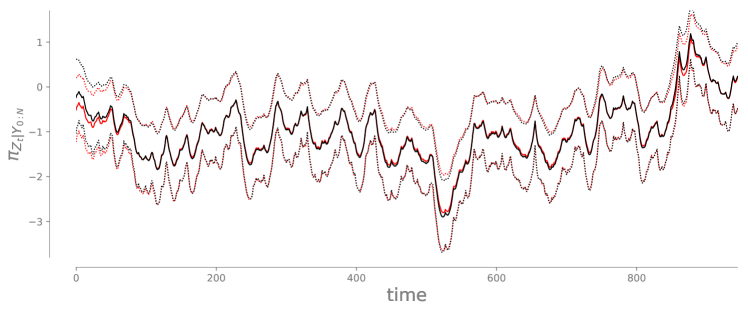
Figure 18: Same as Figure 10, but using linear maps. Compared to a high-order map, there seems to be only a minimal loss of accuracy, more prominent at earlier times.

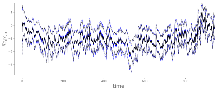
Figure 19: Comparison of the $\{5,95\}$–percentiles (dashed lines) and the mean (solid line) of the numerical approximation of the filtering marginals using linear transport maps (blue lines) with those of a “reference” solution obtained via seventh-order maps (as shown in Figure 11). The two solutions look remarkably similar despite the enormous difference in computational cost (see Table 1).

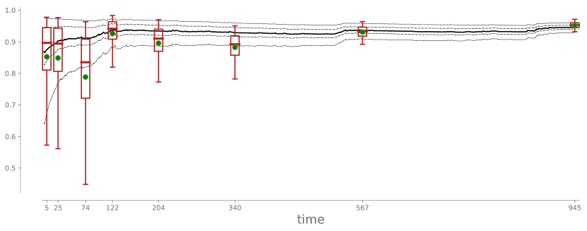
Figure 21: The horizontal plane of Figure 20 (black lines) overlaid with a selected number of box-and-whisker plots associated with the marginals of a “reference” MCMC solution. The ends of the whiskers represent the $\{5,95\}$–percentiles, while the green dots correspond to the means of the reference distribution. Linear maps are insufficient to correctly characterize the parameter marginals, especially the transition at time 74 (cf. Figures 12 and 20)

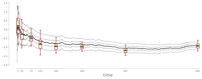
Figure 23: The horizontal plane of Figure 22 (black lines) overlaid with a selected number of box-and-whisker plots associated with the marginals of a “reference” MCMC solution. See Figure 21 caption for more details.

References

- Anderes and Coram [2012] E. Anderes and M. Coram. A general spline representation for nonparametric and semiparametric density estimates using diffeomorphisms. arXiv:1205.5314, 2012.
- Andrieu et al. [2010] C. Andrieu, A. Doucet, and R. Holenstein. Particle Markov chain Monte Carlo methods. Journal of the Royal Statistical Society: Series B, 72(3):269–342, 2010.
- Asmussen and Glynn [2007] S. Asmussen and P. W. Glynn. Stochastic simulation: algorithms and analysis, volume 57. Springer Science & Business Media, 2007.
- Bardsley et al. [2014] J. M. Bardsley, A. Solonen, H. Haario, and M. Laine. Randomize-then-optimize: a method for sampling from posterior distributions in nonlinear inverse problems. SIAM Journal on Scientific Computing, 36(4):A1895–A1910, 2014. doi: 10.1137/140964023.
- Bertsekas [1995] D. P. Bertsekas. Dynamic programming and optimal control, volume 1. Athena Scientific Belmont, MA, 1995.
- Bierman [2006] G. J. Bierman. Factorization methods for discrete sequential estimation. Courier Corporation, 2006.
- Bigoni et al. [2017] D. Bigoni, A. Spantini, and Y. Marzouk. On the computation of monotone transports. In preparation, 2017.
- Blake et al. [2011] A. Blake, P. Kohli, and C. Rother. Markov random fields for vision and image processing. MIT Press, 2011.
- Blei et al. [2016] D. Blei, A. Kucukelbir, and J. McAuliffe. Variational inference: a review for statisticians. arXiv:1601.00670, 2016.
- Bogachev et al. [2005] V. I. Bogachev, A. V. Kolesnikov, and K. V. Medvedev. Triangular transformations of measures. Sbornik: Mathematics, 196(3):309, 2005.
- Bottou et al. [2016] L. Bottou, F. Curtis, and J. Nocedal. Optimization methods for large-scale machine learning. arXiv:1606.04838, 2016.
- Boyd [2001] J. Boyd. Chebyshev and Fourier spectral methods. Dover, 2 edition, 2001.
- Carlier et al. [2010] G. Carlier, A. Galichon, and F. Santambrogio. From Knothe’s transport to Brenier’s map and a continuation method for optimal transport. SIAM Journal on Mathematical Analysis, 41(6):2554–2576, 2010.
- Cheng et al. [2015] D. Cheng, Y. Cheng, Y. Liu, R. Peng, and S. Teng. Efficient sampling for Gaussian graphical models via spectral sparsification. In Conference on Learning Theory, pages 364–390, 2015.
- Chopin et al. [2013] N. Chopin, P. Jacob, and O. Papaspiliopoulos. SMC2: an efficient algorithm for sequential analysis of state space models. Journal of the Royal Statistical Society: Series B (Statistical Methodology), 75(3):397–426, 2013.
- Chorin and Tu [2009] A. J. Chorin and X. Tu. Implicit sampling for particle filters. Proceedings of the National Academy of Sciences, 106(41):17249–17254, 2009.
- Constantine et al. [2014] P. G. Constantine, E. Dow, and Q. Wang. Active subspace methods in theory and practice: Applications to kriging surfaces. SIAM Journal on Scientific Computing, 36(4):A1500–A1524, 2014.
- Crisan and Doucet [2002] D. Crisan and A. Doucet. A survey of convergence results on particle filtering methods for practitioners. IEEE Transactions on signal processing, 50(3):736–746, 2002.
- Crisan and Miguez [2013] D. Crisan and J. Miguez. Nested particle filters for online parameter estimation in discrete-time state-space Markov models. arXiv:1308.1883, 2013.
- Csilléry et al. [2010] K. Csilléry, M. G. B. Blum, O. E. Gaggiotti, and O. François. Approximate Bayesian Computation (ABC) in practice. Trends in ecology & evolution, 25(7):410–8, 2010.
- Cui et al. [2014] T. Cui, J. Martin, Y. Marzouk, A. Solonen, and A. Spantini. Likelihood-informed dimension reduction for nonlinear inverse problems. Inverse Problems, 30(11):114015, 2014.
- Daum and Huang [2008] F. Daum and J. Huang. Particle flow for nonlinear filters with log-homotopy. In SPIE Defense and Security Symposium, pages 696918–696918. International Society for Optics and Photonics, 2008.
- Daum and Huang [2012] F. Daum and J. Huang. Particle flow and Monge-Kantorovich transport. In Information Fusion (FUSION), 2012 15th International Conference on, pages 135–142. IEEE, 2012.
- Davis and Rabinowitz [2007] P. J. Davis and P. Rabinowitz. Methods of numerical integration. Courier Corporation, 2007.
- Del Moral [2004] P. Del Moral. Feynman-Kac formulae. In Feynman-Kac Formulae: Genealogical and Interacting Particle Systems with Applications, pages 47–93. Springer, 2004.
- Del Moral et al. [2017] P. Del Moral, A. Jasra, and Y. Zhou. Biased online parameter inference for state-space models. Methodology and Computing in Applied Probability, 19(3):727–749, 2017.
- Detommaso et al. [2018] G. Detommaso, T. Cui, Y. Marzouk, R. Scheichl, and A. Spantini. A Stein variational Newton method. arXiv:1806.03085, 2018.
- Dick et al. [2013] J. Dick, F. Y. Kuo, and I. H. Sloan. High-dimensional integration: the Quasi-Monte Carlo way. Acta Numerica, 22:133–288, 2013.
- Dick et al. [2016] J. Dick, R. N. Gantner, Q. T. L. Gia, and C. Schwab. Higher order Quasi-Monte Carlo integration for Bayesian estimation. arXiv:1602.07363, 2016.
- Dinh et al. [2016] L. Dinh, J. Sohl-Dickstein, and S. Bengio. Density estimation using Real NVP. arXiv:1605.08803, 2016.
- Doucet and Johansen [2009] A. Doucet and A. M. Johansen. A tutorial on particle filtering and smoothing: Fifteen years later. Handbook of nonlinear filtering, 12(656-704):3, 2009.
- Douglas [1999] R. J. Douglas. Applications of the Monge-Ampere equation and Monge transport problem to meteorology and oceanography. In Monge Ampère Equation: Applications to Geometry and Optimization, volume 226, page 33. American Mathematical Soc., 1999.
- Durbin and Koopman [2000] J. Durbin and S. J. Koopman. Time series analysis of non-Gaussian observations based on state-space models from both classical and Bayesian perspectives. Journal of the Royal Statistical Society: Series B, 62(1):3–56, 2000.
- Erol et al. [2017] Y. B. Erol, Y. Wu, L. Li, and S. J. Russell. A nearly-black-box online algorithm for joint parameter and state estimation in temporal models. In AAAI, pages 1861–1869, 2017.
- Evensen [2003] G. Evensen. The ensemble Kalman filter: Theoretical formulation and practical implementation. Ocean dynamics, 53(4):343–367, 2003.
- Evensen [2007] G. Evensen. Data Assimilation. Springer, 2007.
- Evensen and Van Leeuwen [2000] G. Evensen and P. J. Van Leeuwen. An ensemble Kalman smoother for nonlinear dynamics. Monthly Weather Review, 128(6):1852–1867, 2000.
- Fremlin [2000] D. H. Fremlin. Measure Theory, volume 4. Torres Fremlin, 2000.
- Gaspari and Cohn [1999] G. Gaspari and S. E. Cohn. Construction of correlation functions in two and three dimensions. Quarterly Journal of the Royal Meteorological Society, 125(554):723–757, 1999.
- George and Liu [1989] A. George and J. W. H. Liu. The evolution of the minimum degree ordering algorithm. SIAM Review, 31(1):1–19, 1989.
- Glasserman [1991] P. Glasserman. Gradient estimation via perturbation analysis. Springer Science & Business Media, 1991.
- Glynn [1990] P. W. Glynn. Likelihood ratio gradient estimation for stochastic systems. Communications of the ACM, 33(10):75–84, 1990.
- Godsill et al. [2004] S. J. Godsill, A. Doucet, and M. West. Monte Carlo smoothing for nonlinear time series. Journal of the American Statistical Association, 99(465):156–168, 2004.
- Goodfellow et al. [2014] I. Goodfellow, J. Pouget-Abadie, M. Mirza, B. Xu, D. Warde-Farley, S. Ozair, A. Courville, and Y. Bengio. Generative adversarial nets. In Advances in Neural Information Processing Systems, pages 2672–2680, 2014.
- Goodfellow et al. [2016] I. Goodfellow, Y. Bengio, A. Courville, and Y. Bengio. Deep learning, volume 1. MIT press Cambridge, 2016.
- Hamill et al. [2001] T. M. Hamill, J. S. Whitaker, and C. Snyder. Distance-dependent filtering of background error covariance estimates in an ensemble Kalman filter. Monthly Weather Review, 129(11):2776–2790, 2001.
- Hammersley and Clifford [1971] J. M. Hammersley and P. Clifford. Markov fields on finite graphs and lattices. Unpublished manuscript, 1971.
- Han and Liu [2017] J. Han and Q. Liu. Stein variational adaptive importance sampling. arXiv:1704.05201, 2017.
- Heng et al. [2015] J. Heng, A. Doucet, and Y. Pokern. Gibbs flow for approximate transport with applications to Bayesian computation. arXiv:1509.08787, 2015.
- Ho and Cao [1983] Y. C. Ho and X. Cao. Perturbation analysis and optimization of queueing networks. Journal of Optimization Theory and Applications, 40(4):559–582, 1983.
- Hyvärinen [2005] A. Hyvärinen. Estimation of non-normalized statistical models by score matching. Journal of Machine Learning Research, 6(Apr):695–709, 2005.
- Jacob [2015] P. E. Jacob. Sequential Bayesian inference for implicit hidden Markov models and current limitations. ESAIM: Proceedings and Surveys, 51:24–48, 2015.
- Jog and Loh [2015] V. Jog and P. Loh. On model misspecification and KL separation for Gaussian graphical models. In IEEE International Symposium on Information Theory, pages 1174–1178, 2015.
- Johnson and Willsky [2008] J. K. Johnson and A. S. Willsky. A recursive model-reduction method for approximate inference in Gaussian Markov random fields. IEEE Transactions on Image Processing, 17(1):70–83, 2008.
- Kantas et al. [2015] N. Kantas, A. Doucet, S. S. Singh, J. Maciejowski, and N. Chopin. On particle methods for parameter estimation in state-space models. Statistical Science, 30(3):328–351, 2015.
- Kantorovich [1965] L. V. Kantorovich. The best use of economic resources. Oxford & London: Pergamon Press., 1965.
- Kim et al. [1998] S. Kim, N. Shephard, and S. Chib. Stochastic volatility: likelihood inference and comparison with ARCH models. The Review of Economic Studies, 65(3):361–393, 1998.
- Kingma and Welling [2013] D. P. Kingma and M. Welling. Auto-encoding variational Bayes. arXiv:1312.6114, 2013.
- Kitagawa [1987] G. Kitagawa. Non-Gaussian state-space modeling of nonstationary time series. Journal of the American Statistical Association, 82(400):1032–1041, 1987.
- Kitagawa [1998] G. Kitagawa. A self-organizing state-space model. Journal of the American Statistical Association, pages 1203–1215, 1998.
- Knothe [1957] H. Knothe. Contributions to the theory of convex bodies. The Michigan Mathematical Journal, 4(1):39–52, 1957.
- Koller and Friedman [2009] D. Koller and N. Friedman. Probabilistic graphical models: principles and techniques. MIT press, 2009.
- Kushner and Yin [2003] H. Kushner and G. G. Yin. Stochastic approximation and recursive algorithms and applications, volume 35. Springer Science & Business Media, 2003.
- Laparra et al. [2011] V. Laparra, G. Camps-Valls, and J. Malo. Iterative Gaussianization: from ICA to random rotations. IEEE transactions on neural networks, 22(4):537–549, 2011.
- Lauritzen [1996] S. L. Lauritzen. Graphical Models. Oxford University Press, 1996.
- Law et al. [2015] K. Law, A. Stuart, and K. Zygalakis. Data assimilation: a mathematical introduction, volume 62. Springer, 2015.
- Lin et al. [2015] L. Lin, M. Drton, and A. Shojaie. High-dimensional inference of graphical models using regularized score matching. arXiv:1507.00433, 2015.
- Liu and West [2001] J. Liu and M. West. Combined parameter and state estimation in simulation-based filtering. In Sequential Monte Carlo methods in practice, pages 197–223. Springer, 2001.
- Liu and Wang [2016] Q. Liu and D. Wang. Stein variational gradient descent: a general purpose Bayesian inference algorithm. In Advances in Neural Information Processing Systems, pages 2370–2378, 2016.
- M. et al. [2012] Matthias M., Xuemin T., Ethan A., and Alexandre J. C. A random map implementation of implicit filters. Journal of Computational Physics, 231(4):2049–2066, 2012.
- Marin et al. [2012] J. M. Marin, P. Pudlo, C. P. Robert, and R. J. Ryder. Approximate Bayesian computational methods. Statistics and Computing, 22(6):1167–1180, 2012.
- Marsaglia and Tsang [2000] G. Marsaglia and W. W. Tsang. The ziggurat method for generating random variables. Journal of Statistical Software, 5(8):1–7, 2000.
- Marzouk et al. [2016] Y. Marzouk, T. Moselhy, M. Parno, and A Spantini. Sampling via measure transport: An introduction. In Handbook of Uncertainty Quantification, R. Ghanem, D. Higdon, and H. Owhadi, editors. Springer, 2016.
- Meinshausen and Bühlmann [2006] N. Meinshausen and P. Bühlmann. High-dimensional graphs and variable selection with the Lasso. The Annals of Statistics, pages 1436–1462, 2006.
- Mendoza et al. [2018] M. Mendoza, A. Allegra, and T. P. Coleman. Bayesian Lasso posterior sampling via parallelized measure transport. arXiv:1801.02106, 2018.
- Meng and Schilling [2002] X. Meng and S. Schilling. Warp bridge sampling. Journal of Computational and Graphical Statistics, 11(3):552–586, 2002.
- Mohamed and Lakshminarayanan [2016] S. Mohamed and B. Lakshminarayanan. Learning in implicit generative models. arXiv:1610.03483, 2016.
- Morrison et al. [2017] R. Morrison, R. Baptista, and Y. Marzouk. Beyond normality: Learning sparse probabilistic graphical models in the non-Gaussian setting. Advances in Neural Information Processing Systems, 2017. arXiv:1711.00950.
- Morzfeld et al. [2015] M. Morzfeld, X. Tu, J. Wilkening, and A. Chorin. Parameter estimation by implicit sampling. Communications in Applied Mathematics and Computational Science, 10(2):205–225, 2015.
- Moselhy and Marzouk [2012] T. Moselhy and Y. Marzouk. Bayesian inference with optimal maps. Journal of Computational Physics, 231(23):7815–7850, 2012.
- Oksendal [2013] B. Oksendal. Stochastic differential equations: an introduction with applications. Springer Science & Business Media, 2013.
- Oliver [2015] D. S. Oliver. Metropolized randomized maximum likelihood for sampling from multimodal distributions. arXiv:1507.08563, 2015.
- Parno [2015] M. Parno. Transport maps for accelerated Bayesian computation. PhD thesis, Massachusetts Institute of Technology, 2015.
- Parno and Marzouk [2018] M. Parno and Y. Marzouk. Transport map accelerated Markov chain Monte Carlo. SIAM/ASA Journal on Uncertainty Quantification, 6(2):645–682, 2018.
- Parno et al. [2016] M. Parno, T. Moselhy, and Y. Marzouk. A multiscale strategy for Bayesian inference using transport maps. SIAM/ASA Journal on Uncertainty Quantification, 4(1):1160–1190, 2016.
- Polson et al. [2008] N. G. Polson, J. R. Stroud, and P. Müller. Practical filtering with sequential parameter learning. Journal of the Royal Statistical Society: Series B, 70(2):413–428, 2008.
- Raanes [2016] P. N. Raanes. On the ensemble Rauch-Tung-Striebel smoother and its equivalence to the ensemble Kalman smoother. Quarterly Journal of the Royal Meteorological Society, 142(696):1259–1264, 2016.
- Ramsay [1998] J. O. Ramsay. Estimating smooth monotone functions. Journal of the Royal Statistical Society: Series B, pages 365–375, 1998.
- Ranganath et al. [2014] R. Ranganath, S. Gerrish, and D. M. Blei. Black box variational inference. In Artificial Intelligence and Statistics, pages 814–822, 2014.
- Rauch et al. [1965] H. E. Rauch, C. T. Striebel, and F. Tung. Maximum likelihood estimates of linear dynamic systems. AIAA Journal, 3(8):1445–1450, 1965.
- Reich [2011] S. Reich. A dynamical systems framework for intermittent data assimilation. BIT Numerical Mathematics, 51(1):235–249, 2011.
- Reich [2013] S. Reich. A nonparametric ensemble transform method for Bayesian inference. SIAM Journal on Scientific Computing, 35(4):A2013–A2024, 2013.
- Reich and Cotter [2013] S. Reich and C. Cotter. Ensemble filter techniques for intermittent data assimilation. Large Scale Inverse Problems. Computational Methods and Applications in the Earth Sciences, 13:91–134, 2013.
- Reich and Cotter [2015] S. Reich and C. Cotter. Probabilistic Forecasting and Bayesian Data Assimilation. Cambridge University Press, 2015.
- Rezende and Mohamed [2015] D. J. Rezende and S. Mohamed. Variational inference with normalizing flows. arXiv:1505.05770, 2015.
- Robert and Casella [2013] C. Robert and G. Casella. Monte Carlo statistical methods. Springer Science & Business Media, 2013.
- Rosenblatt [1952] M. Rosenblatt. Remarks on a multivariate transformation. The Annals of Mathematical Statistics, pages 470–472, 1952.
- Rudin [1987] W. Rudin. Real and complex analysis. Tata McGraw-Hill Education, 1987.
- Rue and Held [2005] H. Rue and L. Held. Gaussian Markov random fields: theory and applications. CRC Press, 2005.
- Rue et al. [2009] H. Rue, S. Martino, and N. Chopin. Approximate Bayesian inference for latent Gaussian models by using integrated nested Laplace approximations. Journal of the Royal Statistical Society: Series B, 71(2):319–392, 2009.
- Saad [2003] Y. Saad. Iterative Methods for Sparse Linear Systems. SIAM, 2003.
- Samarov [1993] A. M. Samarov. Exploring regression structure using nonparametric functional estimation. Journal of the American Statistical Association, 88(423):836–847, 1993.
- Santambrogio [2015] F. Santambrogio. Optimal Transport for Applied Mathematicians, volume 87. Springer, 2015.
- Särkkä [2013] S. Särkkä. Bayesian Filtering and Smoothing, volume 3. Cambridge University Press, 2013.
- Schillings and Schwab [2016] C. Schillings and C. Schwab. Scaling limits in computational Bayesian inversion. ESAIM: Mathematical Modelling and Numerical Analysis, 50(6):1825–1856, 2016.
- Shapiro [2013] A. Shapiro. Sample Average Approximation, pages 1350–1355. Springer US, Boston, 2013.
- Smith et al. [2013] A. Smith, A. Doucet, N. de Freitas, and N. Gordon. Sequential Monte Carlo methods in practice. Springer Science & Business Media, 2013.
- Spall [2005] J. C. Spall. Introduction to stochastic search and optimization: estimation, simulation, and control, volume 65. John Wiley & Sons, 2005.
- Spantini [2017] A. Spantini. On the low-dimensional structure of Bayesian inference. PhD thesis, Massachusetts Institute of Technology, 2017.
- Spantini et al. [2015] A. Spantini, A. Solonen, T. Cui, J. Martin, L. Tenorio, and Y. Marzouk. Optimal low-rank approximations of Bayesian linear inverse problems. SIAM Journal on Scientific Computing, 37(6):A2451–A2487, 2015.
- Spantini et al. [2017] A. Spantini, T. Cui, K. Willcox, L. Tenorio, and Y. M. Marzouk. Goal-oriented optimal approximations of Bayesian linear inverse problems. SIAM Journal on Scientific Computing, 39(5):S167–S196, 2017.
- Spivak [1965] M. Spivak. Calculus on manifolds, volume 1. WA Benjamin New York, 1965.
- Stavropoulou and Müller [2015] F. Stavropoulou and J. Müller. Parametrization of random vectors in polynomial chaos expansions via optimal transportation. SIAM Journal on Scientific Computing, 37(6):A2535–A2557, 2015.
- Stuart [2010] A. M. Stuart. Inverse problems: a Bayesian perspective. Acta Numerica, 19:451–559, 2010.
- Tabak and Turner [2013] E. G. Tabak and C. V. Turner. A family of nonparametric density estimation algorithms. Communications on Pure and Applied Mathematics, 66(2):145–164, 2013.
- Tao [2011] T. Tao. An introduction to measure theory, volume 126. American Mathematical Soc., 2011.
- Villani [2008] C. Villani. Optimal transport: old and new, volume 338. Springer Science & Business Media, 2008.
- Wang and Meng [2016] L. Wang and X. Meng. Warp bridge sampling: the next generation. arXiv:1609.07690, 2016.
- Wilkinson [2011] D. J. Wilkinson. Stochastic modelling for systems biology. CRC press, 2011.
- Wright and Nocedal [1999] S. J. Wright and J. Nocedal. Numerical Optimization, volume 2. Springer New York, 1999.
- Xiu [2010] D. Xiu. Numerical methods for stochastic computations: a spectral method approach. Princeton University Press, 2010.
- Yang et al. [2013] T. Yang, P. G. Mehta, and S. P. Meyn. Feedback particle filter. IEEE transactions on Automatic control, 58(10):2465–2480, 2013.
- Yannakakis [1981] M. Yannakakis. Computing the minimum fill-in is NP-complete. SIAM Journal on Algebraic Discrete Methods, 2(1):77–79, 1981.
- Yuan and Lin [2007] M. Yuan and Y. Lin. Model selection and estimation in the Gaussian graphical model. Biometrika, 94(1):19–35, 2007.