A UV Complete Compositeness Scenario: LHC Constraints Meet The Lattice

Abstract

We investigate a recently proposed UV-complete composite Higgs scenario in the light of the first LHC runs. The model is based on a $\text{SU}(4)$ gauge group with global flavour symmetry breaking $\text{SU}(5)\to\text{SO}(5)$, giving rise to pseudo Nambu-Goldstone bosons in addition to the Higgs doublet. This includes a real and a complex electroweak triplet with exotic electric charges. Including these, as well as constraints on other exotic states, we show that LHC measurements are not yet sensitive enough to significantly constrain the model’s low energy constants. The Higgs potential is described by two parameters which are on the one hand constrained by the LHC measurement of the Higgs mass and Higgs decay channels and on the other hand can be computed from correlation functions in the UV-complete theory. Hence to exclude the model at least one constant needs to be determined and to validate the Higgs potential both constants need to be reproduced by the UV-theory. Due to its UV-formulation, a certain number of low energy constants can be computed from first principle numerical simulations of the theory formulated on a lattice, which can help in establishing the validity of this model. We assess the potential impact of lattice calculations for phenomenological studies, as a preliminary step towards Monte Carlo simulations.

I Introduction

The discovery of a Standard Model (SM) like Higgs boson has so far not revealed concrete hints towards an understanding of the electroweak symmetry breaking (EWSB). The concept of Higgs naturalness stands questioned in many established BSM scenarios such as supersymmetry but also in theories of Higgs compositeness. It is conceivable that future LHC runs, exploring higher energy scales with large statistics, will improve the situation. Due to the non-perturbative nature of the composite Higgs models, their phenomenological investigations are typically informed by means of effective theories, in a way that is completely analogous to the description of the low energy dynamics of QCD by chiral perturbation theory. Although these methods have been very successful in understanding the low energy properties of QCD, the ultimate goal is obviously to analyse the phenomenological properties of a composite Higgs scenario by investigating concrete UV-complete candidate theories using non-perturbative techniques to gain a more complete picture of their dynamics from first principles.

The minimal composite Higgs model (MCHM) Contino et al. (2003); Agashe et al. (2005); Contino et al. (2007a) based on global symmetry breaking pattern $\text{SO}(5)\to\text{SO}(4)$ is the prototype of composite Higgs model. The four arising Nambu-Goldstone bosons (NGBs) transform as a bi-doublet under $\text{SU}(2)\times\text{SU}(2)\simeq\text{SO}(4)$ and can therefore be identified with the Higgs doublet in the SM. Breaking the global symmetry by gauging the weak interaction $\text{SU}(2)_{L}\times\text{U}(1)_{Y}\subset\text{SO}(4)$ in the presence of heavy composite fermions induces a Higgs potential. Whether or not the potential triggers EWSB can only be investigated for definite in a UV complete scenario. The scale of the composite sector is parametrised by $f$ and its value compared to $v$, $\xi\equiv v^{2}/f^{2}$ ($v\simeq 246~{}\text{GeV}$ and $\xi\leq 0.12$, e.g. Aad et al. (2015a)), is a measure of the misalignment of the new strong sector and the Higgs sector vacuum. Low energy scenarios based on this symmetry breaking pattern have been scrutinised in the literature in detail Espinosa et al. (2010); Azatov and Galloway (2013); Azatov et al. (2012); Espinosa et al. (2012), however, no UV complete realisation of this minimal scenario has been established so far (see e.g. Ref. Elander et al. (2014) for related work in the holographic context).

Recently Ferretti, in Ref. Ferretti (2014), proposed a UV complete model based on a $\text{SU}(4)$ (hypercolor) gauge symmetry with a flavour structure motivated by partial compositeness, gauge anomaly cancellation and asymptotic freedom Ferretti and Karateev (2014). Earlier UV-complete realisations of the (partial) composite Higgs scenarios are based on embedding effective four fermion operators into gauge theory Barnard et al. (2014) or non-negligible irrelevant operators of SM and composite fermions Vecchi (2017).

This model is distinct, and non-minimal, as compared to MCHM4/5 in that the flavour structure predicts a number of extra pseudo NGBs (PNGB). In this work we reflect on the potential impact of lattice studies on the Higgs sector (e.g. Higgs potential, mass spectrum, …) and investigate the LHC phenomenology of the exotic extra PNGBs. The combined analyses of Higgs measurements and LHC constraints on exotics allows us to identify a region of parameter space of the model, which can be cross checked against lattice calculations. This provides an important guideline for future efforts to construct, modify, simulate and validate UV-complete models of Higgs compositeness. Pioneering lattice studies DeGrand et al. (2016a, b) have shown that these simulations are computationally demanding, therefore strengthening the case for a detailed understanding of the lattice measurements that will be relevant for phenomenology.

This work is organised as follows: In Sec. II we briefly summarise the model of Ferretti (2014) to make this work self-contained. The relevant low energy constants (LECs) which can be computed on the lattice are discussed and identified. Subsequently, in Sec. III we study the model with available LHC Higgs measurements, for which preliminary results have been presented in Del Debbio et al. (2017a), and include constraints from searches for predicted exotic states, which have so far not been discussed in the literature. We summarise and conclude in Sec. IV.

II Ferretti’s model

Ferretti’s model Ferretti (2014) is a gauge theory with hypercolour gauge group $G_{\text{HC}}=\text{SU}(4)$ with 5 massless Weyl fermions transforming in the two-index antisymmetric representation of $G_{\text{HC}}$, and 3 massless Dirac fermions in the fundamental representation of color. Using Weyl fermions, we denote these fermions $\psi,\chi,\tilde{\chi}$ respectively, with $\psi\in\bf{6}$ and $\chi\in\bf{4},\tilde{\chi}\in\bar{\bf{4}}$ under $G_{\text{HC}}$. The theory has a global symmetry group

$$G_{F}=\text{SU}(5)\times\text{SU}(3)\times\text{SU}(3)^{\prime}\times\text{U}(1)_{X}\times\text{U}(1)^{\prime}\,.$$ (II.1)

The strong dynamics of $G_{\text{HC}}$ is expected to break the global flavour symmetries $\text{SU}(5)\to\text{SO}(5)$ and $\text{SU}(3)\times\text{SU}(3)^{\prime}\to\text{SU}(3)_{c}$, as well as $\text{U}(1)_{X}$. The maximally attractive channel hypothesis Raby et al. (1980) suggests $\text{SU}(5)\to\text{SO}(5)$ to occur at a higher scale than $\text{SU}(3)\times\text{SU}(3)^{\prime}\to\text{SU}(3)_{c}$. This leads to a low-energy effective theory based on the global symmetry breaking pattern

$$G_{F}/H_{F} ={\text{SU}(5)\times\text{SU}(3)\times\text{SU}(3)^{\prime}\times\text{U}(1)_{X}\times\text{U}(1)^{\prime}\over\text{SO}(5)\times\text{SU}(3)\times\text{U}(1)_{X}}$$

$$={\text{SU}(5)\over\text{SO}(5)}\times{\text{SU}(3)\times\text{SU}(3)^{\prime}\over\text{SU}(3)}\times\text{U}(1)^{\prime}\,.$$ (II.2)

Since $\text{SO}(5)\supset\text{SO}(4)\simeq\text{SU}(2)\times\text{SU}(2)$, the unbroken global symmetry group $H_{F}$ contains the custodial subgroup

$$H_{c}=\text{SU}(2)_{L}\times\text{SU}(2)_{R}\,.$$ (II.3)

Following the standard paradigm of composite Higgs scenarios, the SM subgroup $G_{\text{SM}}\equiv\text{SU}(3)_{c}\times\text{SU}(2)_{L}\times\text{U}(1)_{Y}\subset H_{F}$ is weakly gauged and the hypercharge is a linear combination of $\text{SU}(2)_{R}$ and $\text{U}(1)_{X}$, $Y=T_{R}^{3}+X$. Weakly gauging a subgroup and heavy quark mass generation through partial compositeness Kaplan (1991); Contino et al. (2007b) amount to explicit violation of $G_{F}$, and the analysis of the one-loop effective action Ferretti (2014) shows that this indeed gives rise to NGB misalignment and EWSB $\text{SU}(2)_{L}\times\text{U}(1)_{Y}\to\text{U}(1)_{\text{QED}}$, in a way that is completely analogous to the minimal effective realisations Agashe et al. (2005, 2006); Contino et al. (2007a). The difference between the MCHM4/5 scenario of Contino et al. (2007a) is the prediction of 14 NGBs from the $\text{SU}(5)\to\text{SO}(5)$ breaking. The NGBs fields are denoted by $\Pi$, classified according to their $\text{SU}(2)_{L}\times\text{U}(1)_{Y}$ quantum numbers $\Pi=(\eta,H,\Phi_{0},\Phi)\in{\mathbf{1}}_{0}+{\mathbf{2}}_{\pm 1/2}+{\mathbf{3}}_{0}+{\mathbf{3}}_{\pm 1}$ and the ${\bf{2}}_{\pm 1/2}$ is identified as the SM Higgs doublet. In this work we investigate the phenomenology of the triplet states but ignore the NGB-singlets $\eta$ mentioned above and $\eta^{\prime}$ due to $\text{U}(1)^{\prime}$-breaking whose phenomenology has been scrutinised in  Ferretti (2016); Belyaev et al. (2017).

This extended scalar sector reveals parallels with the so-called Georgi-Machacek model Georgi and Machacek (1985); Chanowitz and Golden (1985); Gunion et al. (1990) (for recent phenomenological investigations see also Englert et al. (2013); Bambhaniya et al. (2015); Logan and Rentala (2015); Degrande et al. (2016); Hartling et al. (2015)), which also predicts the appearance of a real as well as a complex $\text{SU}(2)_{L}$ triplet in the scalar sector. Whether or not these extra states contribute to the breaking of electroweak symmetry, as in the Georgi-Machacek model, is an interesting open question to be addressed in future research (see e.g. Golterman and Shamir (2017) for similar considerations). We will follow Ferretti’s original ansatz where the triplet states do not contribute to electroweak symmetry breaking. The construction of the low-energy effective theory follows the approach pioneered by Callen, Coleman, Wess and Zumino (CCWZ)  Coleman et al. (1969); Callan et al. (1969). Denoting the $\text{SU}(5)/\text{SO}(5)$ generators by $T^{\hat{A}}$, a non-linear sigma field is introduced

$$\Sigma(x)=\exp\left({i\Pi\over f}\right)\,,~{}\Pi=\phi^{\hat{A}}(x)T^{\hat{A}}\,,$$ (II.4)

transforming non-linearly $\Sigma\to\mathrm{g}\,\Sigma\,\mathrm{h}$ since $\mathrm{h}\in\text{SO}(5)$ is $\Pi$- and $\mathrm{g}$-dependent. The quantity $f\equiv f_{\text{SU}(5)/\text{SO}(5)}$ is the $\Pi$ decay constant which can be thought of as setting the scale of the hypercolour gauge theory. Since $\text{SU}(5)/\text{SO}(5)$ is a symmetric space, the CCWZ kinetic term, governing the interactions with the gauge bosons, is simplified to

$${\cal{L}}\supset{f^{2}\over 16}\text{Tr}\left(D_{\mu}UD^{\mu}U^{\dagger}\right)\,,$$ (II.5)

where $U=\Sigma\Sigma^{T}=\exp(2i\Pi/f)$ transforms linearly $U\mapsto\mathrm{g}\,U\mathrm{g}^{T}$ under $\mathrm{g}\in\text{SU}(5)$. The covariant derivative is given by

$$D_{\mu}U=\partial_{\mu}U-igW^{A}_{\mu}[T^{A}_{L},U]-ig^{\prime}B_{\mu}[T^{3}_{R},U]\,,$$ (II.6)

as all NGBs have zero $\text{U}(1)_{X}$ charge. With the convention ${\text{tr}}[T^{A}T^{B}]=\delta^{AB}/2$ and $\Pi\supset H^{+}T^{+}=H^{+}\sqrt{2}(T^{18}-iT^{15})$, Eq. (II.5) leads to canonically normalised kinetic terms.

Expanding this Lagrangian we find the standard MCHM4/5 coupling modifications of the physical Higgs boson to the massive electroweak gauge bosons rescaled by $\sqrt{1-\xi}$, where $\xi\equiv v^{2}/f^{2}$, while the remaining PNGB interactions are completely determined by their $\text{SU}(2)_{L}$ quantum numbers.

Heavy third family quark masses are included through partial compositeness Kaplan (1991); Contino et al. (2007b), i.e. mixing effects with vector-like hyperbaryons of the strongly interacting sector. The relevant terms originating from an extended HC (EHC) sector are

$$-{\cal{L}}\supset{M}\bar{\Psi}\Psi+\lambda_{q}f\bar{\hat{q}}_{L}\Sigma\Psi_{R}+\lambda_{t}f\bar{\hat{t}}_{R}\Sigma^{\ast}\Psi_{L}\\ +\sqrt{2}\mu_{b}\text{Tr}(\bar{\hat{q}}_{L}^{3}U\hat{d}^{3}_{R})+\text{h.c.}$$ (II.7)

where we introduced the field $\Psi$ to represent the composite fermion in the effective theory, transforming under a $\bf{5}$ of $\text{SO}(5)$ and a $\bf{3}$ of $\text{SU}(3)_{c}$, and $\hat{q}_{L}\supset(t_{L},b_{L})$, and $\hat{t}_{R}\supset t_{R}$ are $\text{SO}(5)$-spurionic embeddings of the third generation quarks. The field $\Psi$ can be written in terms of its components that have definite quantum numbers under the standard model gauge group $\text{SU}(3)_{c}\times\text{SU}(2)\times\text{U}(1)$:

$$\Psi =\frac{1}{\sqrt{2}}[iB-iX,B+X,iT+iY,-T+Y,\sqrt{2}iR]\,,$$ (II.8)

where the quantum numbers are $(T,B)\in(\mathbf{3},\mathbf{2})_{1/6}$, $R\in(\mathbf{3},\mathbf{1})_{2/3}$, and $(X,Y)\in(\mathbf{3},\mathbf{2})_{7/6}$. Expanding this Lagrangian yields a mass matrix in the top partner space $(t,T,Y,R)$:

$$\hat{{\cal{M}}}_{T}=\\ \left(\begin{matrix}0&{\lambda_{q}\over 2}(1+c_{h})&{\lambda_{q}\over 2}(1-c_{h})&{\lambda_{q}\over\sqrt{2}}s_{h}\\ {\lambda_{t}\over\sqrt{2}}s_{h}&\hat{M}&0&0\\ -{\lambda_{t}\over\sqrt{2}}s_{h}&0&\hat{M}&0\\ \lambda_{t}c_{h}&0&0&\hat{M}\end{matrix}\right)\,,$$ (II.9)

and an analogous matrix in the bottom partner space $(b,B)$:

$$\hat{{\cal{M}}}_{B}=\\ \left(\begin{matrix}\hat{\mu}_{b}s_{h}c_{h}&\lambda_{q}\\ 0&\hat{M}\end{matrix}\right)\,,$$ (II.10)

where hatted quantities, e.g. $\hat{M}\equiv M/f$, are made dimensionless by dividing by the appropriate power of $f$. In the expressions above $c_{h}\equiv\cos(\hat{h})$ and $s_{h}\equiv\sin(\hat{h})$, where $h$ is the physical Higgs in the unitary gauge. Bi-unitary transformations yield the physical top and bottom partner mass spectrum as well as their (non-diagonal) interactions with the Higgs after expanding $s_{h},c_{h}$. Note that the $X$-particle and the Higgs $h$ do not interact at the tree-level. To lowest order in $v$ the top mass ${\cal{O}}(v^{0})$ and bottom mass ${\cal{O}}(v)$ are given by

$$m_{t}\simeq\frac{\sqrt{2}\lambda_{q}\lambda_{t}}{\sqrt{\hat{M}^{2}+\lambda_{q}^{2}}\sqrt{\hat{M}^{2}+\lambda_{t}^{2}}}M$$ (II.11)

and

$$m_{b}\simeq\frac{\hat{M}\hat{\mu}_{b}}{\sqrt{\hat{M}^{2}+\lambda_{q}^{2}}}v\,,$$ (II.12)

where $v=\sin(\langle\hat{h}\rangle)$ has been used in the last equation. It is seen from Eq. (II.12) that $\hat{\mu}_{b}$ essentially acts like a Yukawa coupling for the $b$-quark as in the SM. Eq. (II.11) is inverted to $\lambda_{q}=\lambda_{q}(m_{t})$ for the scan for which we use $m_{t}\simeq 173~{}\text{GeV}$. We use a similar strategy to invert Eq. (II.12) $\mu_{b}=\mu_{b}(m_{b},\lambda_{q})$ with $m_{b}\simeq 4.7~{}\text{GeV}$ as an input. Furthermore, we will require $M>1.5~{}\text{TeV}$ (see below) and leave $f$ as a free parameter.

The SM-like Higgs boson phenomenology is identical to MCHM4/5 but includes the previously mentioned exotically charged NGBs. The masses of the NGBs are radiatively induced, in analogy to the $\pi^{\pm}-\pi^{0}$ mass difference in the SM due to electromagnetic interaction. The leading order expression assumes the form Golterman and Shamir (2015)

$$V=f^{2}\hat{C}_{\rm LR}\left((3g^{2}+g^{\prime 2})\left(2H^{\dagger}H+{16\over 3}\Phi^{\dagger}\Phi\right)+8g^{2}\Phi_{0}^{\dagger}\Phi_{0}\right)\,,$$ (II.13)

where $3g^{2}+g^{\prime 2}\simeq 1.31$ and $g^{2}\simeq 0.40$ and

$$C_{\rm LR}={3\over 16\pi^{2}}\int_{0}^{\infty}\hbox{d}q^{2}\,q^{2}\Pi^{33}_{LR}(q^{2})\,,$$ (II.14)

is an integral over the $\text{SU}(2)_{L}\times\text{SU}(2)_{R}$-correlator

$$i\int{\text{d}}^{4}x\,e^{iq\cdot x}\,\,\langle TJ^{\mu\,a}_{L}(x)\,J^{\mu\,b}_{R}(0)\rangle=\Pi^{ab}_{LR}(q^{2})\,P^{\mu\nu}\,.$$ (II.15)

Above $P^{\mu\nu}=(q^{2}g^{\mu\nu}-q^{\mu}q^{\nu})$, $g^{\mu\nu}={\text{diag}}(1,-1,-1,-1)$ and the chiral currents are in the adjoint flavour representation $2J^{\mu\,a}_{L,R}=\bar{\psi}\gamma^{\mu}(1\mp\gamma^{5})T^{a}\psi$. This current has the right quantum numbers to excite the NGBs and therefore $\lim_{q^{2}\to 0}q^{2}\Pi^{33}_{LR}(q^{2})=f^{2}$ as the lowest term in a $q^{2}$ expansion, which underpins Eq. (II.13). In the next section we will consider further corrections to the Higgs potential for which LHC constraints furnish a value for $\hat{C}_{\rm LR}$. The latter gives a lower bound on the triplet masses $\Phi$ and $\Phi_{0}$. Further low energy exotic states include an $\text{SU}(3)_{c}$ octet hyper-pion, whose mass is estimated to be in the multi-TeV regime Ferrera et al. (2011) and has been investigated phenomenologically in Belyaev et al. (2017).

Lessons from the Lattice and the LHC

Several LECs are accessible by first principle computations, e.g. lattice Monte Carlo simulations, of the UV complete theory. As previously mentioned one might think of $f$, the $\Pi$ decay constant in Eq. (II.4), as setting the scale of the $\text{SU}(4)$-hypercolour theory. In increasing order of complexity LECs of interest are the spectrum of the lowest lying state in a given channel (including the composite baryon mass $\hat{M}$), the quark condensates $\langle\Psi\Psi\rangle$ and $\langle\bar{\chi}\chi\rangle$ with associated decay constants $f$ and $f^{\prime}$, and the Higgs potential parameters $\hat{C}_{\rm LR}$, $\hat{F}_{\textrm{EW}}$ and $\hat{F}_{\textrm{LL}}$resulting from non-trivial correlation functions. Preliminary lattice investigations have already started DeGrand et al. (2016a, b), highlighting the subtleties involved in simulating models with fermions in multiple representations of the gauge groups. The results in this section should help in identifying the lattice measurements that are likely to have a significant phenomenological impact.

Higgs Potential

As discussed above, the Higgs particle is one of the NGBs of the UV complete theory. In the hypercolour theory in isolation, no potential is generated for the NGBs; hence the Higgs potential can only arise from interactions with the SM sector. In particular there are two contributions to the one-loop effective potential: the first one is due to the coupling to the weak gauge bosons (cf. Eq. (II.13)) and the second one to the coupling to the top and the composite fermions. Using the standard composite Higgs potential parametrisation

$$\hat{V}(\hat{h})=\alpha\cos(2\hat{h})-\beta\sin^{2}(2\hat{h})\,,$$ (II.16)

the dimensionless parameters $\alpha$ and $\beta$ are given by

$$\alpha = \frac{1}{2}\hat{F}_{\textrm{LL}}-\hat{c}_{\rm LR}$$

$$\beta = \frac{1}{2}\hat{F}_{\textrm{EW}}-\frac{1}{4}\hat{F}_{\textrm{LL}}\;.$$ (II.17)

The quantities $\hat{c}_{\rm LR}$, $\hat{F}_{\textrm{LL}}$ and $\hat{F}_{\textrm{EW}}$ are related to correlation functions of the UV theory. The quantity $\hat{c}_{\rm LR}\equiv\frac{1}{2}(3g^{2}+g^{\prime 2})\hat{C}_{\rm LR}$ is the previously defined $2$-point function Eq. (II.14) whose evaluation on the lattice is a routine matter. The quantities $\hat{F}_{\textrm{LL}}$ and $\hat{F}_{\textrm{EW}}\equiv\hat{F}_{\textrm{LR}}-2\hat{F}_{\textrm{RR}}$ are related to $4$-point functions as defined in appendix A. Their evaluation is a more complex task for lattice Monte Carlo simulations.

We can now analyse the potential in terms of $\alpha$ and $\beta$, imposing the Higgs mass and direct search constraints, and then discuss the relation of the Higgs sector with the two triplet PNGBs. Up to a constant the potential Eq. (II.16) can be written as

$$\hat{V}(\hat{h})=4\beta(\sin^{2}(\hat{h})-\xi)^{2}\,,\quad$$ (II.18)

with

$$\xi\equiv\frac{v^{2}}{f^{2}}=\sin^{2}(\langle\hat{h}\rangle)=\frac{\alpha+2\beta}{4\beta}\,.$$ (II.19)

The important condition for EWSB, then reads

$$\alpha+2\beta=\hat{F}_{\textrm{EW}}-\hat{c}_{\rm LR}>0\,.$$ (II.20)

Hence, the sign of $\beta$, and its magnitude compared to $\alpha$, are the first constraints that the UV complete theory needs to satisfy.

The $\alpha$-$\beta$ parameter space is shown in Fig. 1 with phenomenologically acceptable values of $\xi\in[0,0.12]$ shown in purple. The Higgs mass is related to the second derivative of the potential

$$\hat{m}_{h}^{2}=\hat{V}^{\prime\prime}(\langle\hat{h}\rangle)=32\beta\xi(1-\xi)=8\beta-2\alpha^{2}/\beta\,,$$ (II.21)

and gives a second constraint, cf. Fig. 1, in the $\alpha$-$\beta$ plane by combining Eqs. (II.19) and (II.21)

$$\frac{m_{h}^{2}}{v^{2}}=32\beta(1-\xi)=8(2\beta-\alpha)\simeq 0.258\,.$$ (II.22)

From Fig. 1, $0.012<-\alpha<0.02$ and $0.06<\beta<0.11$ can be inferred. Note that this range mainly depends on unknown radiative corrections to the Higgs mass.

Further observables are the two triplet $\Phi_{0}\in{\mathbf{3}}_{0}$ and $\Phi\in{\mathbf{3}}_{1}$ (for $\text{SU}(2)_{L}\times U(1)_{Y}$) PNGB masses. At leading order the mass of $\Phi_{0}$ is determined by integrating out the gauge bosons Eq. (II.13); the charged triplet receives a contribution from integrating out the third generation through the $4$-point function $\hat{F}_{\textrm{LL}}$ defined in appendix A,

$$\hat{m}_{\Phi_{0}}^{2} \;=\; 16g^{2}\hat{C}_{\rm LR}\;, \;\simeq\; 0.36^{2}\;,$$ (II.23)

$$\hat{m}_{\Phi}^{2} \;=\; 16(g^{2}+\frac{g^{\prime 2}}{3})\hat{C}_{\rm LR}+8\hat{F}_{\textrm{LL}} \;\simeq\; 0.34^{2}+8\hat{F}_{\textrm{LL}}\,.$$

The triplet masses are equal in the limit where the hypercharge disappears $g^{\prime 2}\to 0$ and the EHC-coupling $\lambda_{1}\to 0$ (cf. appendix A.) In the limit $\hat{F}_{\textrm{LL}}\to 0$ the mass difference of the charged to neutral is positive, $m_{\Phi}-m_{\Phi_{0}}\geq 0$, as for the pions in the SM Witten (1983).

From the LHC bound $\xi=v^{2}/f^{2}<0.12$ it follows that $f\gtrsim 5.7m_{h}$ and therfore

$$m_{\Phi_{0}}>1.97m_{h}\,.$$ (II.24)

A lattice determination of $\hat{C}_{\rm LR}$ ($0.012<-\alpha<0.02$ and $0.06<\beta<0.11$ for our example) together with Eq. (II) allows us to set an upper and lower bound on $\hat{F}_{\textrm{EW}}$ and $\hat{F}_{\textrm{LL}}$. The latter can then be tensioned against triplet mass $m_{\Phi}$ (II.23) and potential lattice determinations of $\hat{F}_{\textrm{EW}}$ and $\hat{F}_{\textrm{LL}}$.

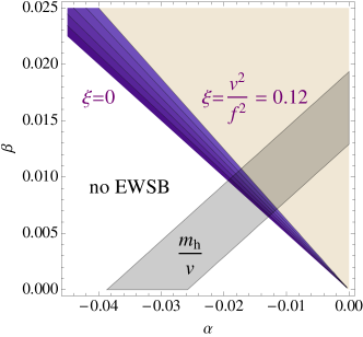
Figure 1: Contour plot for $\xi=(\alpha+2\beta)/(4\beta)$, Eq. (II.19). In the white region no EWSB occurs and the purple level curves are values of $\xi$ ranging from $0$ to $0.12$ where the latter value is a representative constraint taken from Ref. Aad et al. (2015a). An additional constraint comes from the Higgs mass $m_{h}^{2}/v^{2}=8(2\beta-\alpha)\simeq 0.258$, Eq. (II.22), for which we have allowed generous $20\%$ radiative corrections. The intersection of the purple and grey region is the physically allowed parameter space of the model that has to be satisfied by the UV theory.

In summary the Higgs potential is parametrised by the two constants $\alpha$ and $\beta$, Eq. (II.16), which are experimentally constrained by $m_{h}/v$, $v/f$ and the requirement of EWSB. On the other hand $\alpha$ and $\beta$ can be determined from well-defined correlation function of the UV hypercolor theory, Eq. (II). Hence the determination of either $\alpha$ or $\beta$ alone can exclude the model. As previously mentioned and discussed further below the computation of $C_{\rm LR}$ is standard on the lattice whereas the evaluation of $\hat{F}_{\textrm{EW}}$ and $\hat{F}_{\textrm{LL}}$ is far from clear. Since no linear combination of $\alpha$ and $\beta$ is independent of the $4$-functions $\hat{F}_{\textrm{EW}}$ and $\hat{F}_{\textrm{LL}}$ it is therefore not possible for the lattice alone to exclude or validate the model but one needs to take into account further phenomenological consideration discussed in the previous paragraph.

The quantity $C_{\rm LR}$ has been computed recently in DeGrand et al. (2016c) for an $\text{SU}(4)$ gauge theory in the quenched approximation with fermion $N_{f({\bf 6})}=4$ in the two-index antisymmetric representation for which we extract a value of $\hat{c}_{\rm LR}\simeq 0.08$. This can only be considered a rough benchmark value since Ferretti’s model ($N_{f({\bf 6})}=5$ and $N_{f({\bf 4})}=N_{f({\bf\bar{4}})}=3$) differs from theirs ($N_{f({\bf 6})}=4$ and $N_{f({\bf 4})}=N_{f({\bf\bar{4}})}=0$) DeGrand et al. (2016c)). The feasibility of computing $C_{\rm LR}$ on the lattice depends on how quickly the $C_{\rm LR}$-integral Eq. (II.14) saturates in $q^{2}$. One can envision to approach this by either computing $\Pi_{\textrm{LR}}(q^{2})$ for low values of $q^{2}$ observing convergence or saturate the correlator in the hadronic picture with the $J^{\textrm{PC}}=1^{--}$ and $1^{+-}$ $\text{SU}(2)_{L}$-triplet states following the idea of the original Weinberg sum rules Weinberg (1967). The computation of $\hat{F}_{\textrm{EW}}$ and $\hat{F}_{\textrm{LL}}$ is a formidable task which becomes more feasible when integrating out the top quarks at ${\cal{O}}(\alpha_{s}^{0})$ further neglecting the top quark mass. Even in this case the question of convergence of the $4$-point correlation function Del Debbio et al. (2017b) is far from trivial since for instance the EHC sector has not been specified Ferretti (2014). In AdS/CFT inspired 5D-models the Higgs potential is found to be insensitive to the UV-completion Agashe et al. (2005); Contino et al. (2007a). It should be noted that this scenario automatically assumes a large $N_{c}$ limit.

Quark Condensates and Goldstone Boson Decay Constants

Quark condensates are related to the zero eigenvalue density of the Dirac operator via the Banks-Casher relation and can therefore be studied on the lattice. Whereas the order parameter for SSB of the flavour symmetries $\text{SU}(5)\to\text{SO}(5)$ and $\text{SU}(3)\times\text{SU}(3)^{\prime}\to\text{SU}(3)_{c}$ are the corresponding decay constants, a non-zero or zero value of the corresponding fermion-condensates $\langle\Psi\Psi\rangle$ and $\langle\bar{\chi}\chi\rangle$ reveals further information about the mechanism of SSB. Furthermore, this permits the possibility to check the Gell-Mann Oakes Renner relation $f^{\prime 2}m_{\pi}^{2}=2m_{\chi}\langle\bar{\chi}\chi\rangle$ since lattice simulation are performed at finite quark mass in practice. A further possibility is to test the successful Pagels-Stokar relation Pagels and Stokar (1979) based on a fermion self energy of the form $\Sigma(q^{2})\to\Lambda^{3}_{\text{ hadron}}/q^{2}$ for $q^{2}\to\infty$ which can also be motivated from the operator product expansion Politzer (1976).

III Parameter regions after LHC measurements

The UV complete model in this paper comes with a $\text{SU}(5)$ flavour symmetry in the Higgs sector which leads to a number of additional PNGBs, as compared to the MCHM4/5, with exotic charge numbers. More precisely, the model predicts the previously mentioned ${\bf{3}}_{0}$ and ${\bf{3}}_{1}$ states, $\Phi_{0}\supset(\phi_{0}^{-},\phi_{0}^{0},\phi_{0}^{+})$ and $\Phi_{+}\supset(\phi_{+}^{-},\phi_{+}^{0},\phi_{+}^{+})$, where the sum of the $\pm$ and $0$ indices indicate the electric charges $Q=Y+T_{L}^{3}$. Additional exotic particles are the top and bottom partner of the hypercolor theory. The NGBs acquire a mass from integrating out the weak gauge bosons with masses given by Eq. (II.13) from where the ratios to the Higgs masses

The masses of the weak PNGBs are indirectly constrained by the LHC data through $C_{\rm LR}$, Eq. (II.13) which leads to $m_{\Phi},m_{\Phi_{0}}\gtrsim 2m_{h}$ at leading order in the effective theory. Note that at leading order in the effective theory there is no mixing between the two triplet states. We treat $m_{\Psi}$ and $m_{\Psi_{0}}$ as free parameters in our scan in the range $m>200~{}\text{GeV}>m_{h}$. We limit our study to $m<1~{}\text{TeV}$ due to a vanishing LHC sensitivity.

We will focus in this work on direct constraints, but a few comments regarding constraints from electroweak precision observables are in order. As the assignment of top partner quantum numbers is analogous to that of MCHM5, the right-left symmetry required to avoid tension with non-oblique $Zb\bar{b}$ measurements Agashe et al. (2006) is also present in this model and the discussion of gauge and fermion contributions to the oblique parameters follows Refs. Agashe and Contino (2006); Agashe et al. (2006); Lodone (2008); Gillioz (2009); Anastasiou et al. (2009). In particular, the numerical analysis of Ref. Gillioz et al. (2012) suggests that electroweak precision constraints can be satisfied over a broad range of values of $\xi$. We can expect the impact of the additional scalars to be further suppressed compared to the top partners. Since they do not contribute to electroweak symmetry breaking, their loop contribution to the $2$-point electroweak bosons’ polarisation functions is entirely due to their gauge interactions. Hence the constraints from oblique corrections do only constrain the mass splittings between the custodial quintet, triplet and singlets. Due to Eq. (II.24) we can expect these contributions to be small.

Constraints from coloured Exotica

The LHC analysis programme that targets the phenomenology of the fermionic partners of Eq. (II.8) is well-developed across a range of final states (see e.g. Aad et al. (2012) or Sirunyan et al. (2016)). A comprehensive interpretation of searches for exotic top partner spectra as detailed above has been performed recently in Ref. Matsedonskyi et al. (2016). In particular, searches for the baryon $X$, with exotic charge $5/3$, set constraints on the vector-like mass $M\gtrsim 1.5~{}\text{TeV}$. We include this constraint to our scan directly.

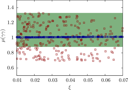
(a)  $\gamma\gamma$ signal strength.

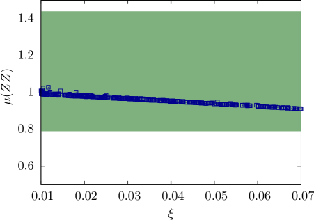
(b)  $ZZ$ signal strength.

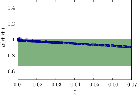
(c)  $WW$ signal strength.

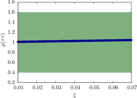
(d)  $\tau\tau$ signal strength.

Figure 2: 125 GeV Higgs signal strengths as constrained by the ATLAS and CMS combination of Ref. Aad et al. (2016a). The blue-shaded area corresponds to the points in our scan yielding the correct top and bottom masses. The red points in panel (a) result from a modified scan which includes the charged exotic Higgs loop contributions to the diphoton partial decay width, demonstrating that the signal strength in the photon channel can be significantly impacted by the presence of these states. The scatter in the red points results from varying the sign and size of the unknown trilinear Higgs couplings.

Searches for pair-produced colour-octet scalars $\pi^{a}$, as predicted from the breaking to QCD in Eq. (II.2) $\text{SU}(3)\times\text{SU}(3)^{\prime}\to\text{SU}(3)_{c}$ with subsequent gauging of QCD, have been considered in theories of vector-like confinement Kilic et al. (2010); Kilic and Okui (2010); Schumann et al. (2011), compositeness Hayot and Napoly (1981); Ellis et al. (1981); Belyaev et al. (1999); Bai and Martin (2010); Ferretti (2016), as well as in hybrid SUSY models Plehn and Tait (2009); Choi et al. (2009). Searches were performed during Run-1 Aad et al. (2013); Khachatryan et al. (2015a) in four jet final states as well as in R-parity violating SUSY scenarios Aad et al. (2016b). CMS have published a search using first 13 TeV data which pushes constraints into the multi-TeV regime Khachatryan et al. (2016a). None of the analyses have reported anomalies or even evidence; the $\pi^{a}$ color octet mass is therefore pushed to $m_{\pi^{a}}\gtrsim 3.5~{}\text{TeV}$ by using the results of Khachatryan et al. (2016a) (assuming $\text{BR}=1$). While this scale is important information for non-perturbative analyses (e.g. Bizot et al. (2016)), it does not impact the model’s phenomenology in the weak sector. A comprehensive analysis of the phenomenology of these states was presented recently in Ref. Belyaev et al. (2017).

Constraints from Higgs signal strengths

As already mentioned, the phenomenology of the 125 GeV SM-like Higgs boson follows largely the MCHM4/5 paradigm, with one crucial difference related to the potential appearance of additional charged exotic Higgs bosons which could modify the Higgs signal strengths, which we define as

$$\mu={\sigma\text{BR}\over[\sigma\text{BR}]^{\text{SM}}}\,.$$ (III.1)

$\sigma$ and BR denote the production cross section and branching ratios for $gg\to\Phi\to(WW,ZZ,\gamma\gamma,\tau\tau)$ respectively. We will limit ourselves to the dominant gluon fusion production mode in this work. The signal strengths are relatively precisely determined quantities after Run-1 Aad et al. (2016a) (see also Aad et al. (2015a) for an interpretation of ATLAS results in terms of composite models).

In Fig.  2, we show a scan over the model following the prescription as detailed earlier. As can be seen, the current Higgs signal strength measurements are consistent with the model’s prediction over a large range of values of $\xi=v^{2}/f^{2}$. In this sense our findings are consistent with the analysis of Aad et al. (2015a). However, the possibility of additional charged scalars running in the $h\to\gamma\gamma$ loops can significantly change this result. Given the early stage of the Higgs phenomenology programme, the Higgs measurements are not sensitive enough to provide tight constraints on the model.

Constraints from exotic Higgs searches

Doubly Charged Scalars

The most striking BSM signature related to the exotic Higgs states is the production of doubly charged scalars. Since the triplet states’ potential is not affected by electroweak symmetry breaking, these states can only be pair-produced as $W^{+}W^{+}\phi^{-}_{-}$ vertices are absent in the effective theory. This leads to a qualitatively different phenomenology compared to one of the standard scenarios of scalar weak triplets Georgi and Machacek (1985); Chanowitz and Golden (1985); Gunion et al. (1990): In our case, the dominant production mechanism relevant for the LHC is Drell-Yan production (with expected moderate QCD corrections $K\simeq 1.3$ see e.g. Hamberg et al. (1991)) which is entirely determined by the hypercharge and $\text{SU}(2)_{L}$ quantum numbers of the doubly charged scalar. For a choice $m_{\phi^{\pm}_{\pm}}=200~{}\text{GeV}$, we obtain a Drell-Yan cross section of $84~{}\text{fb}$, which decreases exponentially for heavier masses.

Current analyses Aad et al. (2015b); Chatrchyan et al. (2012) set constraints mostly from searches for same-sign lepton production, which are motivated from a Majorana-type lepton sector operators involving the ${\bf{3}}_{1}$ multiplet in the Georgi-Machacek model Georgi and Machacek (1985); Gunion et al. (1990). Although leptons are not included in Ferretti’s proposal Ferretti (2014), we can expect the biggest coupling to arise from $\tau$ leptons following the partial compositeness paradigm. Ref. Chatrchyan et al. (2012) sets a constraint in this channel of $\sim 100~{}\text{fb}$, which is not stringent enough to constrain the presence of a doubly charged Higgs boson as predicted in the model even when we consider decays to $\tau$ leptons.

If this lepton operator is not considered, the dominant decay will be to same sign $W$ bosons via fermion loops Englert et al. (2016). Ref. Aad et al. (2015b) does not make any specific assumptions on jet or missing energy activity and set constraints of $\sim 1~{}\text{fb}$. Including the $W$ branching fractions the weak pair production of the doubly-charged scalar in our model readily evades these constraints. The recent analysis Englert et al. (2016) that specifically targets the $pp\to 4\ell+\text{missing energy}$ smoking signature shows that the LHC should in principle be able to probe a mass regime up to 700 GeV.

Charged Scalars

Charged Higgs boson searches have been performed during Run-1 by ATLAS Aad et al. (2016c) and CMS Khachatryan et al. (2015b) from the production off top quarks and set constraints of $0.6$-$0.8~{}\text{pb}$ in the considered mass region. In our scan, we find cross sections in the range of $\simeq 1~{}\text{fb}$ after averaging between the 4 and 5 flavour scheme as detailed in Harlander et al. (2011). W conclude that available LHC analyses are not sensitive enough to constrain the exotic Higgs spectrum because of the small production cross section.

Neutral Scalars

The interactions of Eq. (II.7) also introduces Yukawa-type interactions with the heavy SM fermions and top partners after diagonalisation of Eqs. (II.9) and (II.10). The dominant production modes of the extra neutral scalars is then gluon fusion with heavy SM fermions and top partners running in the gluon fusion loops.

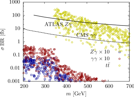
Figure 3: Scan over the neutral, CP even ${\bf{3}}_{1}$ state including ATLAS The ATLAS Collaboration (2016a) and CMS Khachatryan et al. (2015c, 2016b). Currently no model-independent LHC constraint exists for the $\bar{t}t$-channel.

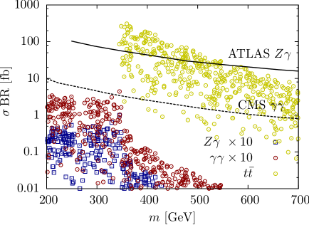
Figure 4: Scan over the neutral, CP odd ${\bf{3}}_{1}$ state including ATLAS The ATLAS Collaboration (2016a) and CMS Khachatryan et al. (2015c, 2016b). Currently no model-independent LHC constraint exists for the $\bar{t}t$-channel.

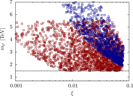
(a)  Mass of the lightest top partner.

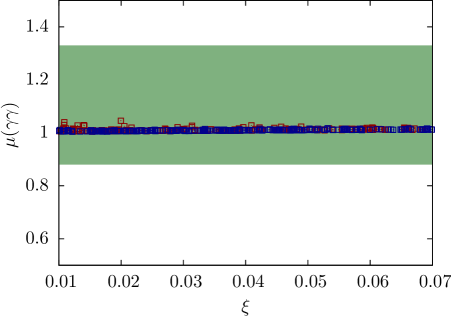
(b)  Diphoton signal strength.

Figure 5: Contour plot for a scan of the first non-SM top partner in agreement with the current LHC constraints (dashed line) detailed in Sec. III (a) and diphoton Higgs signal strength (b). Blue points show the correlation expected from a lattice result of $\hat{M}\in[2,5]$ while the red points leave $M$ as a free parameter in $M\in[1.5,5.5]~{}\text{TeV}$.

We calculate the gluon fusion cross sections, for the parameters that reproduce the correct top and bottom masses, which satisfy constraints of the current top partners outlined above as well as the 125 GeV Higgs measurements. A flat QCD $K\simeq 1.6$ factor Dawson (1991); Kauffman and Schaffer (1994); Graudenz et al. (1993); Spira (1995); Spira et al. (1995) is included.

Since the ${\bf{3}}_{0}$ state couples to $\sim\lambda_{q}\bar{b}_{L}B_{R}/\sqrt{2}+{\text{h.c.}}$ the phase space enhanced decay into physical bottom quarks dominates, irrespective of the smallness of the coupling. For these final states there are currently no sensitive searches given the large expected QCD backgrounds and the challenge of triggering such final states in the first place.

Loop-induced decays (see Appendix B) to $\gamma\gamma$ are already fairly constrained after Run-1. For instance, CMS limit $\sigma{\text{Br}}(\gamma\gamma)\lesssim 1$-$10~{}\text{fb}$ between 180 and 800 GeV with little dependence on the resonance width Khachatryan et al. (2015c) (see also the analysis by ATLAS Aad et al. (2014a) with similar sensitivity). CMS have updated their results also including 13 TeV data Khachatryan et al. (2016b), which mostly extends the sensitivity region up to $m\simeq 4~{}\text{TeV}$ with limits $\sigma{\text{Br}}(\gamma\gamma)\lesssim 0.2~{}\text{fb}$ for $m>2~{}\text{TeV}$. Numerically we find the diphoton branching ratios to be suppressed by three orders of magnitude compared to $b\bar{b}$ for the ${\bf{3}}_{0}$ state in our scan, which leaves it unconstrained by these measurements (identical conclusions hold for other loop-induced decays).

The neutral ${\bf{3}}_{1}$ states do not couple to bottom quarks but both CP-even and odd interactions follow from the operator $\sim\sqrt{2}\lambda_{q}\,\bar{t}_{L}Y_{r}+{\text{h.c}}$. This opens up the interesting phenomenological possibilities below the $t\bar{t}$ threshold. We find that for such a mass choice the decay into gluons typically dominates. However, it is worthwhile to also check the sensitivity to these states in other final states, also extending beyond the aforementioned diphoton analysis.

The production of $Z\gamma$ final states was constrained in Run-1 analyses Chatrchyan et al. (2013); Aad et al. (2014b), which focused on mass ranges inspired by the SM $m\lesssim 190~{}\text{GeV}$ with only weak constraints $\sigma\text{BR}(Z\gamma)\lesssim 100~{}\text{fb}$. ATLAS and CMS have extended these searches to the higher mass regime The ATLAS Collaboration (2016a); The CMS Collaboration (2016) with 13 TeV data and set limits ${\cal{O}}(10)~{}\text{fb}$ above 300 GeV. The hierarchy in branching ratios, however, makes neither the diphoton searches nor the $Z\gamma$ analyses sensitive enough to impose mass limits on the considered CP even state, Fig. 3.

Searches for $ZZ$ and $WW$ decays, which are also mediated at the loop level are available Khachatryan et al. (2015d); The ATLAS Collaboration (2016b) and constrain signal strengths of $\sim 10\%$ relative to the SM expectation. These searches are not yet sensitive enough to constrain this scenario.

A similar conclusion holds for the CP odd state as the increase in production cross sections is not sizable enough to make current constraints sensitive to the model. The bulk of the considered parameter space is left constraint with the early 13 TeV data, Fig. 4. Once the $t\bar{t}$ channel becomes accessible as a decay mode, the loop-induced decays become unconstrained for scalar masses above $2m_{t}$.

If the mass of the neutral scalar lies above the top mass threshold, the decay to top pairs becomes kinematically accessible and will dominate over the loop-induced diboson decays. Searches for the CP even or odd scalar resonances in $t\bar{t}$ final states exist in the context of two Higgs doublet models The ATLAS Collaboration (2016c). Although this analysis is difficult to interpret in our scenario due to the involved signal-background interference, the sensitivity in this search probes $\tan\beta\simeq 1$, which corresponds to a signal cross section of around 0.15 pb around 500 GeV which quickly decreases for larger masses. As can be seen from Figs. 3 and 4, this search will start to constrain the parameter space, although the spread of points shows that there is still a large range parameter points where the model remains viable, in particular for larger masses.

Ignoring systematic uncertainties in extrapolating the results to the high luminosity target of 3/ab, the CMS $\gamma\gamma$ analysis should significantly constrain the presence of extra scalars in the spectrum below the $t\bar{t}$ threshold as the exclusion contour will be become a factor $\sim 15$ more stringent. A similar conclusion holds for the $t\bar{t}$ channel although details will depend on signal background interference.

In summary, we find that while there are searches at the LHC which might become sensitive to the exotic states predicted by the model of Sec. II in the near future, current analyses are not yet constraining enough to significantly limit the models parameter space. This can be understood as a motivation to explore this scenario on the lattice as valid candidate theory of TeV scale compositeness.

Finally, coming back to the potential impact of lattice input, we show the scan of top partners assuming a lattice calculation input of $\hat{M}$. This results in a correlation of the top partner spectrum with $f$, Fig. 5 and indicates that an observation of top partners in the near future at the LHC can not only provide an input to a more comprehensive investigation on the lattice, but, more importantly can potentially rule out the model of Eqs. (II.1) and (II.2) directly.

IV Summary and Conclusions

The observation of a SM-like Higgs and no additional evidence of physics beyond the SM provides no hint towards a more fundamental theory of the TeV scale.

Non-minimal theories of Higgs compositeness have always been attractive solutions to solve this puzzle, but recently they have received particular attention as the possibility of UV-complete models paves the way for applying non-perturbative techniques. Such a programme needs to be informed by the results of the LHC as collider constraints can be understood in terms of the UV-theory’s LECs. In this work, we provide the latest constraints from Higgs-like measurements as well as from searches for additional pseudo Nambu-Goldstone weak triplets with exotic charges predicted by the scenario of Ferretti (2014).

Including constraints from the literature on the exotic states that are relevant for our analysis of LECs of this particular scenario, we find that the latter is largely unconstrained at this stage in the LHC programme. Extrapolating to $3/\text{ab}$, the weak exotics searches are capable of limiting the effective theory’s parameter space. In particular, the increasing precision on the 125 GeV Higgs couplings (see e.g. Bock et al. (2011); Klute et al. (2013); Englert et al. (2014)) will allow us to explore the coupling strength deviations in the $5\%$-range, which will provide stringent constraints (see Fig. 2) on the model.

Direct searches are not constraining on the top partner mass $m_{t}^{\prime}$ but when combined with lattice determinations the situation may change. For instance, the prediction of the hypercolor baryon mass $M$, in units of the decay constants $f$, provides directly falsifiable predictions on the top quark partner spectra as shown in Fig. 5. In the longer term, the computation of the Higgs potential parameters $\alpha$ and $\beta$ provides first principle constraints on the viability of the model against the Higgs mass and Higgs decay channel measurements (cf. Fig. 1). In particular the determination of only one of these parameters can exclude the model whereas both parameters are needed to confirm it in this sector. The lattice technology developed within this particular model can be used for future UV completions that may become interesting in the future.

Acknowledgments — We thank Tom DeGrand, Gabriele Ferretti, Marc Gillioz, Maarten Golterman, and Yigal Shamir for helpful discussions and especially Gabriele Ferretti for relevant comments on the draft. In particular we would like to thank Maarten Golterman, and Yigal Shamir for informing us about the possibility of further $4$-point function corrections to the Higgs potential. LDD and RZ are supported by the UK STFC grants ST/L000458/1 and ST/P000630/1. LDD is supported by the Royal Society, Wolfson Research Merit Award, grant WM140078.

Appendix A Four point-functions

The Higgs potential arises from integrating out the gauge bosons using the Coleman-Weinberg method (giving rise to $C_{\rm LR}$) and involves the effective top and bottom quark couplings to the hypercolour-baryon. The contributions of the latter are given by 4-point correlator functions

$$F_{\textrm{LR}} = -(\lambda_{1}\lambda_{2})^{2} \int_{x_{1,2,3}}\langle J_{\bar{L}Ri}(x_{1},x_{2})J^{\dagger}_{\bar{L}Rk}(x_{3},x_{4})\rangle_{i\neq k}\;,$$

$$F_{\textrm{RR}} = -\lambda_{2}^{4}\times \int_{x_{1,2,3}}\langle J_{RRi}(x_{1},x_{2})J^{\dagger}_{RRk}(x_{3},x_{4})\rangle_{i\neq k}\;,$$

$$F_{\textrm{LL}} = -\lambda_{1}^{4}\times \int_{x_{1,2,3}}\langle J_{LLi}(x_{1},x_{2})J^{\dagger}_{LLk}(x_{3},x_{4})\rangle_{i\neq k}\;,$$ (A.1)

where $F_{\textrm{LR}}=-y^{2}C_{\text{top}}$ in the notation of Ref. Golterman and Shamir (2015), and where we have defined the short-hand notation $\int_{x_{1,2,3}}=\int d^{4}x_{1}\,d^{4}x_{2}\,d^{4}x_{3}$. The bi-local currents in Eq. (A.1) are defined as

$$J_{\bar{L}Ri}(x_{1},x_{2}) \;=\; \bar{t}_{L}{\cal B}_{i}(x_{1})\bar{\cal B}_{i}t_{R}(x_{2})\;,$$

$$J_{RRi}(x_{1},x_{2}) \;=\; \bar{\cal B}_{i}(x_{1})t_{R}\bar{\cal B}_{i}t_{R}(x_{2})\;,$$

$$J_{LLi}(x_{1},x_{2}) \;=\; \bar{\cal B}_{i}(x_{1})t_{L}\bar{\cal B}_{i}t_{L}(x_{2})\;.$$

The latter originate from the (E)HC interaction

$${\cal L}_{\textrm{EHC}}=\lambda_{1}\bar{\hat{q}}_{L}{\cal B}_{R}+\lambda_{2}\bar{\hat{q}}_{R}{\cal B}_{L}+\textrm{h.c.}\;,$$

with $\hat{q}_{L,R}=T_{L,R}$ in the notation of Ref. Golterman and Shamir (2015). The hypercolour-baryon operator is given by

$${\cal B}_{Ria}=-\frac{1}{2}\epsilon^{ABCD}\epsilon_{abc}P_{R}\psi_{ABi}\chi^{T}_{Cb}CP_{R}\chi_{Dc}\;,$$ (A.2)

where $a,b,c$ are $\text{SU}(3)_{c}$, $A,B,C,D$ are $\text{SU}(4)_{\textrm{HC}}$, and $i$ is a $\text{SO}(5)$ indices. Comparing to the notation of Golterman and Shamir (2015), we use $\chi\leftrightarrow\psi$ in accordance with Ferretti’s original convention. Note that ${\hat{q}}_{L}$ but not $\hat{q}_{R}$ transforms non-trivially under the effective custodial symmetry $SU(2)_{R}$. Therefore $\lambda_{1}$ or $F_{\textrm{LL}}$ are responsible for further splittings of the two isotriplets $SU(2)_{L}$ in Eq. (II.23).

At last we note that in order to obtain a potential which is manifestly $\text{SU}(2)_{L}$ invariant the bottom quarks also needs to be integrated out. The $4$-point function, focusing on the top quark, do though give the right coefficients.

Appendix B Analysis of loop-induced decays of the non-Higgs scalar states

In this section we briefly review the calculation underpinning the loop-induced decays of the additional neutral scalars in the model.

After diagonalising the top- and bottom mass mixing matrices, the scalar as well as vectorial couplings will be in general non-diagonal in the top and bottom partner spaces (and not necessarily purely vectorial)w . This leads to a multi-scale decay amplitude that can be pictorially represented by the sum over Feynman diagrams indicated in Fig. 6.

Figure 6: Representative Feynman diagram mediating the decay of a neutral scalar $S\in\{{\bf{3}}_{0},{\bf{3}}_{1}\}$ to vector bosons $V,V^{\prime}\in\{Z,\gamma,W^{\pm}\}$ with interaction vertices obtained in the mass-diagonal representation of the charged and neutral top and bottom space currents.

We can write the unrenormalised decay amplitude at one loop as

$$i{\cal{A}}=\sum_{i}C_{i}\langle\hat{O}_{i}\rangle$$ (B.1)

with $\hat{O}_{i}$ denoting the quantum operators contributing to the decay with matrix element $\langle\hat{O}_{i}\rangle$ and associated couplings $C_{i}$ (which can have a non-zero mass dimension). In our case the relevant operators are

$$\hat{O}_{1} =\hat{S}\hat{V}^{\mu}\hat{V}^{\prime}_{\mu}\,,$$

$$\hat{O}_{2} =\hat{S}\hat{V}^{\mu\nu}\hat{V}^{\prime}_{\mu\nu}\,,$$

$$\hat{O}_{3} =\hat{S}\hat{V}^{\mu\nu}{\hat{\widetilde{V^{\prime}}}}_{\mu\nu}\,,$$

$\tilde{V}$ denotes the dual field strength tensor.

The latter two operators typically arise from integrating out chiral fermions Kniehl and Spira (1995), while the first one is the standard $V$-Higgs interaction associated with spontaneous symmetry breaking.

Calculating the decay amplitude, one finds that all coefficients in Eq. (B.1) are UV-finite except $C_{1}$. This result is familiar from the SM within which top and bottom loop contributions renormalise the tree-level $HVV$ operators.

There is no such interaction in the EFT for the non-Higgs states and the considered order in chiral perturbation theory due to the symmetry of the underlying UV theory. However, these symmetries are spurious (e.g. leading to $S$ obtaining a mass from a Coleman-Weinberg potential) and quantum corrections will excite all operators that are allowed by explicitly intact symmetries. Hence, they will also excite the absent operator $\hat{O}_{1}$.

It is interesting to mention another similarity with the $\text{SU}(2)_{L}$ triplet scenario of Georgi and Machacek (1985) here. In this model, the requirement of custodial invariance identifies the real and complex $\text{SU}(2)_{L}$ triplet vacuum expectation value. This identification is broken at the quantum level signalised by the appearance of additional UV singularities that require the introduction of independent bare quantities Gunion et al. (1991) (while the renormalised quantities can be identified as input to the renormalisation procedure).

From a technical perspective the problem encountered in the calculation of the decay amplitude is similar. We are forced to introduce a bare operator $\hat{O}_{1}$ and supply the underlying UV physics through a renormalisation condition (as part of a minimal set of EFT input parameters). The counter term amplitude in our case can be written as (using $C_{1}=C_{1}^{R}+\delta Z_{C_{1}}$ and multiplicative renormalisation of the quantum fields) turns Eq. (B.1) into using

$$i{\cal{A}}=(C_{1}+\delta Z_{C})\langle\hat{O}_{1}\rangle^{R}+\dots$$ (B.2)

with the ellipses denoting finite terms $\sim\langle\hat{O}_{1,2}\rangle$.

To reflect the symmetry breaking pattern that underpins our EFT formulation, we need to provide input data to the renormalisation procedure. This is guided by the EFT not allowing the dimension three operator due to the approximate shift symmetry of the Nambu-Goldstone $S$. All interactions generated by loops that violate this symmetry (and eventually creates a mass of $S$) are higher order in the EFT expansion Giudice et al. (2007); Kniehl and Spira (1995). A suitable renormalisation condition is therefore a vanishing coefficient $C^{R}_{1}=0$. This fixes the renormalisation constant $\delta Z_{C_{1}}$ and renders the amplitude UV finite.

References

- Contino et al. (2003) R. Contino, Y. Nomura, and A. Pomarol, Nucl. Phys. B671, 148 (2003), eprint hep-ph/0306259.
- Agashe et al. (2005) K. Agashe, R. Contino, and A. Pomarol, Nucl. Phys. B719, 165 (2005), eprint hep-ph/0412089.
- Contino et al. (2007a) R. Contino, L. Da Rold, and A. Pomarol, Phys. Rev. D75, 055014 (2007a), eprint hep-ph/0612048.
- Aad et al. (2015a) G. Aad et al. (ATLAS), JHEP 11, 206 (2015a), eprint 1509.00672.
- Espinosa et al. (2010) J. R. Espinosa, C. Grojean, and M. Muhlleitner, JHEP 05, 065 (2010), eprint 1003.3251.
- Azatov and Galloway (2013) A. Azatov and J. Galloway, Int. J. Mod. Phys. A28, 1330004 (2013), eprint 1212.1380.
- Azatov et al. (2012) A. Azatov, R. Contino, and J. Galloway, JHEP 04, 127 (2012), [Erratum: JHEP04,140(2013)], eprint 1202.3415.
- Espinosa et al. (2012) J. R. Espinosa, C. Grojean, M. Muhlleitner, and M. Trott, JHEP 12, 045 (2012), eprint 1207.1717.
- Elander et al. (2014) D. Elander, A. F. Faedo, C. Hoyos, D. Mateos, and M. Piai, JHEP 05, 003 (2014), eprint 1312.7160.
- Ferretti (2014) G. Ferretti, JHEP 06, 142 (2014), eprint 1404.7137.
- Ferretti and Karateev (2014) G. Ferretti and D. Karateev, JHEP 03, 077 (2014), eprint 1312.5330.
- Barnard et al. (2014) J. Barnard, T. Gherghetta, and T. S. Ray, JHEP 02, 002 (2014), eprint 1311.6562.
- Vecchi (2017) L. Vecchi, JHEP 02, 094 (2017), eprint 1506.00623.
- DeGrand et al. (2016a) T. A. DeGrand, D. Hackett, W. I. Jay, E. T. Neil, Y. Shamir, and B. Svetitsky, PoS LATTICE2016, 219 (2016a), eprint 1610.06465.
- DeGrand et al. (2016b) T. A. DeGrand, M. Golterman, W. I. Jay, E. T. Neil, Y. Shamir, and B. Svetitsky, Phys. Rev. D94, 054501 (2016b), eprint 1606.02695.
- Del Debbio et al. (2017a) L. Del Debbio, C. Englert, and R. Zwicky (2017a), eprint 1702.05417.
- Arkani-Hamed et al. (2002) N. Arkani-Hamed, A. G. Cohen, E. Katz, and A. E. Nelson, JHEP 07, 034 (2002), eprint hep-ph/0206021.
- Terazawa et al. (1977) H. Terazawa, K. Akama, and Y. Chikashige, Phys. Rev. D15, 480 (1977).
- Terazawa (1980) H. Terazawa, Phys. Rev. D22, 184 (1980).
- Raby et al. (1980) S. Raby, S. Dimopoulos, and L. Susskind, Nucl. Phys. B169, 373 (1980).
- Kaplan (1991) D. B. Kaplan, Nucl. Phys. B365, 259 (1991).
- Contino et al. (2007b) R. Contino, T. Kramer, M. Son, and R. Sundrum, JHEP 05, 074 (2007b), eprint hep-ph/0612180.
- Agashe et al. (2006) K. Agashe, R. Contino, L. Da Rold, and A. Pomarol, Phys. Lett. B641, 62 (2006), eprint hep-ph/0605341.
- Ferretti (2016) G. Ferretti, JHEP 06, 107 (2016), eprint 1604.06467.
- Belyaev et al. (2017) A. Belyaev, G. Cacciapaglia, H. Cai, G. Ferretti, T. Flacke, A. Parolini, and H. Serodio, JHEP 01, 094 (2017), eprint 1610.06591.
- Georgi and Machacek (1985) H. Georgi and M. Machacek, Nucl. Phys. B262, 463 (1985).
- Chanowitz and Golden (1985) M. S. Chanowitz and M. Golden, Phys. Lett. B165, 105 (1985).
- Gunion et al. (1990) J. F. Gunion, R. Vega, and J. Wudka, Phys. Rev. D42, 1673 (1990).
- Englert et al. (2013) C. Englert, E. Re, and M. Spannowsky, Phys. Rev. D87, 095014 (2013), eprint 1302.6505.
- Bambhaniya et al. (2015) G. Bambhaniya, J. Chakrabortty, J. Gluza, T. Jelinski, and R. Szafron, Phys. Rev. D92, 015016 (2015), eprint 1504.03999.
- Logan and Rentala (2015) H. E. Logan and V. Rentala, Phys. Rev. D92, 075011 (2015), eprint 1502.01275.
- Degrande et al. (2016) C. Degrande, K. Hartling, H. E. Logan, A. D. Peterson, and M. Zaro, Phys. Rev. D93, 035004 (2016), eprint 1512.01243.
- Hartling et al. (2015) K. Hartling, K. Kumar, and H. E. Logan, Phys. Rev. D91, 015013 (2015), eprint 1410.5538.
- Golterman and Shamir (2017) M. Golterman and Y. Shamir (2017), eprint 1707.06033.
- Coleman et al. (1969) S. R. Coleman, J. Wess, and B. Zumino, Phys. Rev. 177, 2239 (1969).
- Callan et al. (1969) C. G. Callan, Jr., S. R. Coleman, J. Wess, and B. Zumino, Phys. Rev. 177, 2247 (1969).
- Golterman and Shamir (2015) M. Golterman and Y. Shamir, Phys. Rev. D91, 094506 (2015), eprint 1502.00390.
- Ferrera et al. (2011) G. Ferrera, M. Grazzini, and F. Tramontano, Phys. Rev. Lett. 107, 152003 (2011), eprint 1107.1164.
- Foadi et al. (2013) R. Foadi, M. T. Frandsen, and F. Sannino, Phys. Rev. D87, 095001 (2013), eprint 1211.1083.
- Witten (1983) E. Witten, Phys. Rev. Lett. 51, 2351 (1983).
- DeGrand et al. (2016c) T. A. DeGrand, M. Golterman, W. I. Jay, E. T. Neil, Y. Shamir, and B. Svetitsky, Phys. Rev. D94, 054501 (2016c), eprint 1606.02695.
- Weinberg (1967) S. Weinberg, Phys. Rev. Lett. 18, 507 (1967).
- Del Debbio et al. (2017b) L. Del Debbio, C. Englert, and R. Zwicky, in preparation (2017b).
- Pagels and Stokar (1979) H. Pagels and S. Stokar, Phys. Rev. D20, 2947 (1979).
- Politzer (1976) H. D. Politzer, Nucl. Phys. B117, 397 (1976).
- Agashe and Contino (2006) K. Agashe and R. Contino, Nucl. Phys. B742, 59 (2006), eprint hep-ph/0510164.
- Lodone (2008) P. Lodone, JHEP 12, 029 (2008), eprint 0806.1472.
- Gillioz (2009) M. Gillioz, Phys. Rev. D80, 055003 (2009), eprint 0806.3450.
- Anastasiou et al. (2009) C. Anastasiou, E. Furlan, and J. Santiago, Phys. Rev. D79, 075003 (2009), eprint 0901.2117.
- Gillioz et al. (2012) M. Gillioz, R. Grober, C. Grojean, M. Muhlleitner, and E. Salvioni, JHEP 10, 004 (2012), eprint 1206.7120.
- Aad et al. (2012) G. Aad et al. (ATLAS), JHEP 11, 094 (2012), eprint 1209.4186.
- Sirunyan et al. (2016) A. M. Sirunyan et al. (CMS) (2016), eprint 1612.05336.
- Matsedonskyi et al. (2016) O. Matsedonskyi, G. Panico, and A. Wulzer, JHEP 04, 003 (2016), eprint 1512.04356.
- Aad et al. (2016a) G. Aad et al. (ATLAS, CMS) (2016a), eprint 1606.02266.
- Kilic et al. (2010) C. Kilic, T. Okui, and R. Sundrum, JHEP 02, 018 (2010), eprint 0906.0577.
- Kilic and Okui (2010) C. Kilic and T. Okui, JHEP 04, 128 (2010), eprint 1001.4526.
- Schumann et al. (2011) S. Schumann, A. Renaud, and D. Zerwas, JHEP 09, 074 (2011), eprint 1108.2957.
- Hayot and Napoly (1981) F. Hayot and O. Napoly, Z. Phys. C7, 229 (1981).
- Ellis et al. (1981) J. R. Ellis, M. K. Gaillard, D. V. Nanopoulos, and P. Sikivie, Nucl. Phys. B182, 529 (1981).
- Belyaev et al. (1999) A. Belyaev, R. Rosenfeld, and A. R. Zerwekh, Phys. Lett. B462, 150 (1999), eprint hep-ph/9905468.
- Bai and Martin (2010) Y. Bai and A. Martin, Phys. Lett. B693, 292 (2010), eprint 1003.3006.
- Plehn and Tait (2009) T. Plehn and T. M. P. Tait, J. Phys. G36, 075001 (2009), eprint 0810.3919.
- Choi et al. (2009) S. Y. Choi, M. Drees, J. Kalinowski, J. M. Kim, E. Popenda, and P. M. Zerwas, Phys. Lett. B672, 246 (2009), eprint 0812.3586.
- Aad et al. (2013) G. Aad et al. (ATLAS), Eur. Phys. J. C73, 2263 (2013), eprint 1210.4826.
- Khachatryan et al. (2015a) V. Khachatryan et al. (CMS), Phys. Lett. B747, 98 (2015a), eprint 1412.7706.
- Aad et al. (2016b) G. Aad et al. (ATLAS), JHEP 06, 067 (2016b), eprint 1601.07453.
- Khachatryan et al. (2016a) V. Khachatryan et al. (CMS), Phys. Rev. Lett. 116, 071801 (2016a), eprint 1512.01224.
- Bizot et al. (2016) N. Bizot, M. Frigerio, M. Knecht, and J.-L. Kneur (2016), eprint 1610.09293.
- Akeroyd and Moretti (2012) A. G. Akeroyd and S. Moretti, Phys. Rev. D86, 035015 (2012), eprint 1206.0535.
- Hamberg et al. (1991) R. Hamberg, W. L. van Neerven, and T. Matsuura, Nucl. Phys. B359, 343 (1991), [Erratum: Nucl. Phys.B644,403(2002)].
- Christensen and Duhr (2009) N. D. Christensen and C. Duhr, Comput. Phys. Commun. 180, 1614 (2009), eprint 0806.4194.
- Alloul et al. (2014a) A. Alloul, N. D. Christensen, C. Degrande, C. Duhr, and B. Fuks, Comput. Phys. Commun. 185, 2250 (2014a), eprint 1310.1921.
- Alloul et al. (2014b) A. Alloul, N. D. Christensen, C. Degrande, C. Duhr, and B. Fuks, J. Phys. Conf. Ser. 523, 01 (2014b), eprint 1309.7806.
- Degrande et al. (2012) C. Degrande, C. Duhr, B. Fuks, D. Grellscheid, O. Mattelaer, and T. Reiter, Comput. Phys. Commun. 183, 1201 (2012), eprint 1108.2040.
- Alwall et al. (2014) J. Alwall, R. Frederix, S. Frixione, V. Hirschi, F. Maltoni, O. Mattelaer, H. S. Shao, T. Stelzer, P. Torrielli, and M. Zaro, JHEP 07, 079 (2014), eprint 1405.0301.
- Aad et al. (2015b) G. Aad et al. (ATLAS), JHEP 03, 041 (2015b), eprint 1412.0237.
- Chatrchyan et al. (2012) S. Chatrchyan et al. (CMS), Eur. Phys. J. C72, 2189 (2012), eprint 1207.2666.
- Englert et al. (2016) C. Englert, P. Schichtel, and M. Spannowsky (2016), eprint 1610.07354.
- Aad et al. (2016c) G. Aad et al. (ATLAS), JHEP 03, 127 (2016c), eprint 1512.03704.
- Khachatryan et al. (2015b) V. Khachatryan et al. (CMS), JHEP 11, 018 (2015b), eprint 1508.07774.
- Harlander et al. (2011) R. Harlander, M. Kramer, and M. Schumacher (2011), eprint 1112.3478.
- The ATLAS Collaboration (2016a) The ATLAS Collaboration, Tech. Rep. ATLAS-CONF-2016-044, CERN, Geneva (2016a).
- Khachatryan et al. (2015c) V. Khachatryan et al. (CMS), Phys. Lett. B750, 494 (2015c), eprint 1506.02301.
- Khachatryan et al. (2016b) V. Khachatryan et al. (CMS), Submitted to: Phys. Lett. B (2016b), eprint 1609.02507.
- Arnold et al. (2009) K. Arnold et al., Comput. Phys. Commun. 180, 1661 (2009), eprint 0811.4559.
- Hahn and Perez-Victoria (1999) T. Hahn and M. Perez-Victoria, Comput. Phys. Commun. 118, 153 (1999), eprint hep-ph/9807565.
- Hahn (2001) T. Hahn, Comput. Phys. Commun. 140, 418 (2001), eprint hep-ph/0012260.
- Dawson (1991) S. Dawson, Nucl. Phys. B359, 283 (1991).
- Kauffman and Schaffer (1994) R. P. Kauffman and W. Schaffer, Phys. Rev. D49, 551 (1994), eprint hep-ph/9305279.
- Graudenz et al. (1993) D. Graudenz, M. Spira, and P. M. Zerwas, Phys. Rev. Lett. 70, 1372 (1993).
- Spira (1995) M. Spira (1995), eprint hep-ph/9510347.
- Spira et al. (1995) M. Spira, A. Djouadi, D. Graudenz, and P. M. Zerwas, Nucl. Phys. B453, 17 (1995), eprint hep-ph/9504378.
- Aad et al. (2014a) G. Aad et al. (ATLAS), Phys. Rev. Lett. 113, 171801 (2014a), eprint 1407.6583.
- Chatrchyan et al. (2013) S. Chatrchyan et al. (CMS), Phys. Lett. B726, 587 (2013), eprint 1307.5515.
- Aad et al. (2014b) G. Aad et al. (ATLAS), Phys. Lett. B732, 8 (2014b), eprint 1402.3051.
- The CMS Collaboration (2016) The CMS Collaboration, Tech. Rep. CMS-PAS-EXO-16-034, CERN, Geneva (2016).
- Khachatryan et al. (2015d) V. Khachatryan et al. (CMS), JHEP 10, 144 (2015d), eprint 1504.00936.
- The ATLAS Collaboration (2016b) The ATLAS Collaboration, Tech. Rep. ATLAS-CONF-2016-082, CERN, Geneva (2016b).
- The ATLAS Collaboration (2016c) The ATLAS Collaboration, Tech. Rep. ATLAS-CONF-2016-073, CERN, Geneva (2016c).
- Bock et al. (2011) S. Bock, R. Lafaye, T. Plehn, M. Rauch, D. Zerwas, and P. M. Zerwas, Phys. Lett. B694, 44 (2011), eprint 1007.2645.
- Klute et al. (2013) M. Klute, R. Lafaye, T. Plehn, M. Rauch, and D. Zerwas, Europhys. Lett. 101, 51001 (2013), eprint 1301.1322.
- Englert et al. (2014) C. Englert, A. Freitas, M. M. Mühlleitner, T. Plehn, M. Rauch, M. Spira, and K. Walz, J. Phys. G41, 113001 (2014), eprint 1403.7191.
- Kniehl and Spira (1995) B. A. Kniehl and M. Spira, Z. Phys. C69, 77 (1995), eprint hep-ph/9505225.
- Gunion et al. (1991) J. F. Gunion, R. Vega, and J. Wudka, Phys. Rev. D43, 2322 (1991).
- Giudice et al. (2007) G. F. Giudice, C. Grojean, A. Pomarol, and R. Rattazzi, JHEP 06, 045 (2007), eprint hep-ph/0703164.