Wind asymmetry imprint in the UV light curves
of the symbiotic binary SY Mus

Abstract

Context. Light curves (LCs) of some symbiotic stars show a different slope of the ascending and descending branch of their minimum profile. The origin of this asymmetry is not understood well.

Aims. We explain this effect in the ultraviolet LCs of the symbiotic binary SY Mus.

Methods. We model the continuum fluxes in the spectra obtained by the International Ultraviolet Explorer at $10$ wavelengths, from $1280$ to $3080$ Å. We consider that the white dwarf radiation is attenuated by H⁰ atoms, H^- ions and free electrons in the red giant wind. Variation in the nebular component is approximated by a sine wave along the orbit as suggested by spectral energy distribution models. The model includes asymmetric wind velocity distribution and the corresponding ionization structure of the binary.

Results. We determined distribution of the H⁰ and H⁺, as well as upper limits of H^- and H⁰ column densities in the neutral and ionized region at the selected wavelengths as functions of the orbital phase. Corresponding models of the LCs match well the observed continuum fluxes. In this way, we suggested the main UV continuum absorbing (scattering) processes in the circumbinary environment of S-type symbiotic stars.

Conclusions. The asymmetric profile of the ultraviolet LCs of SY Mus is caused by the asymmetric distribution of the circumstellar matter at the near-orbital-plane area.

1 Introduction

Asymmetric light curves (LCs) of some interacting binaries along the orbital phase can be caused by a variety of geometrical and physical effects. For example, by the presence of cool or hot spots/areas (e.g. Bopp & Noah 1980; Bell et al. 1984; Pustylnik et al. 2007; Samec et al. 2009; Yuan 2010; Pribulla et al. 2011), an asymmetric wind distribution in symbiotic binaries (e.g. Dumm et al. 1999), a slopping accretion column (Andronov 1986), pulsation of binary components (Kato et al. 2012; Popper 1961, and references therein), a Coriolis effect (e.g. Zhou & Leung 1990), or an eccentric orbit (Elsner et al. 1980). In the X-ray binaries, the asymmetry of the ascending and descending parts of LCs can originate from a relativistic Doppler effect (Watarai et al. 2005).

The asymmetry of ingress and egress branch of the LCs minimum was also indicated for some symbiotic systems (e.g. Dumm et al. 1999; Kolotilov et al. 2002; Skopal et al. 2002, 2012; Wiecek et al. 2010). These widest interacting binaries comprise usually a red giant (RG) as the donor star and a white dwarf (WD) as the accretor. The binary components interact via the wind mass transfer from the RG to the WD (e.g. Boyarchuk 1967; Mürset & Schmid 1999).

Using a semi-quantitative analysis, Formiggini & Leibowitz (1990) suggested that a reflection effect can account for the wave-like orbitally related variations in the LCs of three symbiotic systems. Analysing long-term photometric observations of a group of classical symbiotic stars, Skopal (1998) revealed apparent changes of their orbital period as a consequence of variable, orbitally related nebular emission. In addition, Skopal (2001) found that the observed amplitudes of the LCs are far larger than those calculated within a model of the reflection effect. For a supersoft X-ray symbiotic binary SMC3, the asymmetry of LCs in the V and I filter and the X-rays was modelled by Kato et al. (2013). They assumed a spiral tail of neutral hydrogen at the orbital plane produced by the giant almost filling in its Roche lobe.

Using a Monte Carlo simulations of the Rayleigh scattering effects in symbiotic stars, Schmid (1995) showed that the eclipse width and depth in ultraviolet (UV) LC profiles depend mainly on the extension of the H⁰ region within the model of Seaquist et al. (1984) (hereafter STB), wavelength and contribution of the scattered light.

SY Mus is a quiet eclipsing symbiotic binary, which shows an asymmetry in its UV LCs. Dumm et al. (1999) demonstrated this effect for the continuum fluxes at 1380 Å. They found that the ascending branch of the LC minimum is less steep than the descending one, and shifted more from the position of the spectroscopic conjunction. Further, measuring the neutral hydrogen column densities around the eclipse of the hot component, they revealed the asymmetric wind density distribution around the giant and suggested this effect to be responsible for the asymmetric UV LC around the eclipse. Recently, Shagatova et al. (2016) derived the velocity profiles of the wind in symbiotic systems SY Mus and EG And and they indicated that the wind from the giant is focused at the orbital plane.

In this work we prove that the observed asymmetry in the UV LC profile is primarily caused by the asymmetrical displacement of the circumbinary matter at the orbital-plane-area with respect to the binary axis. In Sect. 2, we present our dataset and in Sect. 3 we introduce our model. Discussion of results and conclusion are included in Sects. 4 and 5.

2 Observed continuum fluxes of SY Mus

We used 44 SWP and 39 LWP/LWR International Ultraviolet Explorer (IUE) spectra of SY Mus to measure the continuum fluxes at 10 wavelengths from $1280$ to $3080$ Å  (Table 1, available online). The spectra were dereddened with $E_{\rm B-V}=0.35$ mag (Skopal 2005). According to Dumm et al. (1999) we used the ephemeris for the time of the inferior conjunction of the giant as

$$JD_{\rm spec.conj.}=2\,450\,176+625\times E.$$ (1)

The resulting LCs show an asymmetry of their descending and ascending branches and an offset of the minima position with respect to the time of the inferior conjunction of the giant. These effects weaken towards the longer wavelengths (Fig. 7).

3 The model

3.1 Components of the continuum radiation

During quiescent phases, the continuum radiation of S-type (stellar) symbiotic binaries consists of three basic components. Radiation from the WD dominates the far-UV range ($\lambda\lesssim 1800$ Å), whereas the ionized part of the wind, i.e. the symbiotic nebula, represents the main contribution within the near-UV and optical (Fig. 8, bottom). The radiation from the RG dominates the spectrum from around $VRI$ passbands to longer wavelengths, depending on its spectral type (e.g. Skopal 2005). Therefore, we assume the WD and nebula as the only sources of radiation in analysing the UV continuum (120 – 330 nm) of SY Mus. To model the observed orbitally-related flux variation, we use the following assumptions.

• The hot component radiates as a black-body at the temperature $T_{\rm h}=105\,000$ K (Mürset et al. 1991). The radiation is attenuated by the wind material along the line of sight as a function of the orbital phase $\varphi$, and can be expressed as,

  $$F^{\rm h}_{\lambda}(\varphi)=\pi B_{\lambda}(T_{\rm h})e^{-\tau_{\lambda}(\varphi)},$$ (2)

  where $B_{\lambda}(T_{\rm h})$ is Planck function and $\tau_{\lambda}(\varphi)$ is the total optical depth along the line of sight.

• The radiation from the nebula is for the sake of simplicity approximated by a sine wave as,

  $$F^{\rm n}_{\lambda}(\varphi)=\alpha_{\lambda}\sin[2\pi(\varphi-0.25)]+\beta_{\lambda},$$ (3)

  where $\alpha_{\lambda}$ and $\beta_{\lambda}$ are model parameters. This assumption is based on the fact that the nebular continuum varies with the orbital phase (e.g. Fernández-Castro et al. 1988) and is responsible for the wave-like orbitally-related variation observed in the LCs of symbiotic stars during quiescence (Skopal 2001). Their profile along the orbit can be compared to a sine function (for SY Mus, see Fig. 2 of Pereira et al. 1995; Skopal 2009).

The model continuum is then given by their superposition, i.e.,

$$F_{\lambda}(\varphi)=F^{\rm h}_{\lambda}(\varphi)+F^{\rm n}_{\lambda}(\varphi).$$ (4)

3.2 Attenuation in the stellar continuum

In this section, we discuss individual components of the total optical depth, $\tau_{\lambda}(\varphi)$, that attenuates the WD continuum radiation on the line of sight. With respect to the ionization structure of the hydrogen in the binary, we consider attenuation processes in the neutral and ionized part of the giant’s wind. Therefore, $\tau_{\lambda}(\varphi)$ is a sum of the optical depth of the neutral region, $\tau_{\lambda}^{0}(\varphi)$, and that of the ionized region, $\tau_{\lambda}^{+}(\varphi)$, i.e.,

$$\tau_{\lambda}(\varphi)=\tau_{\lambda}^{0}(\varphi)+\tau_{\lambda}^{+}(\varphi).$$ (5)

In a dense H⁰ zone of symbiotic binaries, a strong attenuation of the continuum around the Ly-$\alpha$ line is caused by Rayleigh scattering (Nussbaumer et al. 1989). Further, we consider the scattering on negative hydrogen ion, H^-, that attenuates the stellar radiation in cool atmospheres (e.g. Gray 2005). Thus, we can write,

$$\tau_{\lambda}^{0}(\varphi)=\sigma_{\rm Ray}(\lambda)n_{\rm H^{0}}(\varphi)+\kappa_{\rm H^{-}}(\lambda)n_{\rm H^{-}}(\varphi),$$ (6)

where $\sigma_{\rm Ray}(\lambda)$ is the cross-section of Rayleigh scattering (Eq. 5 and Fig. 2 of Nussbaumer et al. 1989), $n_{\rm H^{0}}(\varphi)$ and $n_{\rm H^{-}}(\varphi)$ is the function for the column density of the neutral hydrogen (Sect. 3.3) and negative hydrogen ion, respectively. The H^- bound-free absorption coefficients, $\kappa_{\rm H^{-}}(\lambda)$, are given by Geltman (1962). We used $\kappa_{\rm H^{-}}(\lambda)$ values from the ”velocity”-curve plotted in his Fig. 6. Corresponding $\kappa_{\rm H^{-}}(\lambda)$ curve reaches its maximum at $\approx 8500$ Å.

We assume that the contribution to the H^- absorption coefficient due to free-free transitions is negligible, considering the absorption coefficient values given in Geltman (1962), Doughty & Fraser (1966) and Gray (2005). The dependence of the H^- column density on the orbital phase, $n_{\rm H^{-}}(\varphi)$, remains a variable in the LC modelling through the neutral region. The values of $\sigma_{\rm Ray}(\lambda)$ and $\kappa_{\rm H^{-}}(\lambda)$ for selected wavelengths are summarized in Table 2. The Rayleigh scattering is the dominant source of opacity in the neutral region at $\lambda=1280$ Å, however, its effect on the WD radiation is comparable with b-f transitions of H^- ion at $\lambda=1340$ Å. At longer wavelengths, these transitions have the dominant attenuating effect in the neutral region (see Fig. 1).

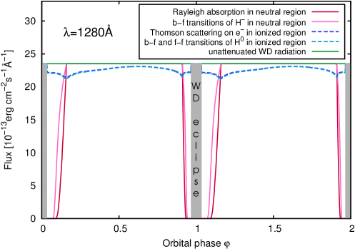
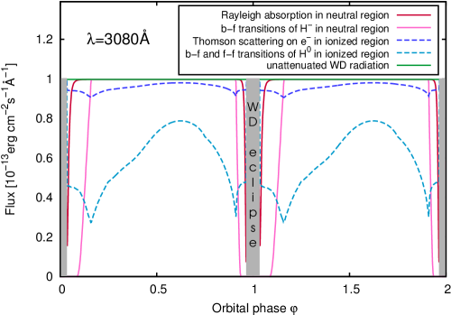
Figure 1: Comparison of the effect of individual considered attenuation processes on the WD flux (Sect. 3.2) at shortest (top) and longest (bottom) wavelength of the set. Corresponding column densities of H⁰ in neutral region and H⁺ in ionized region are given by the column density model in Fig. 6 and of H^- in neutral region and H⁰ in ionized region by the LC modelling (Sect. 4). Two minima of radiation out of the eclipse for attenuation processes in ionized region (dashed lines) correspond to the orbital phase with line of sight entering/exiting the neutral region.

In Eq. (6), Rayleigh scattering is treated as an absorption process. However, the Rayleigh scattered photons can contribute to the line-of-sight continuum radiation. Schmid (1995) used Monte Carlo simulations to determine the percentage of these photons in the total flux. In his model S_B3, corresponding to a typical symbiotic system, with model parameters closest to that of SY Mus, he obtained values of $7.7\%$ at $\lambda=1250$ Å, $1.9\%$ at $\lambda=1350$ Å  and $0.25\%$ at $\lambda=1700$ Å, as seen at the orbital phase $\varphi=0.25$. To estimate this effect in our LC modelling , we fitted his values by a function

$$P(\lambda)=a_{0}+e^{a_{1}(a_{2}-\lambda)},$$ (7)

which represents the percentage of flux from Rayleigh scattered photons in the total modelled flux. This function for resulting values of parameters $a_{0}=0.241$, $a_{1}=0.015$ Å^-1 and $a_{2}=1383,66$ Å  is depicted in Fig. 2 and evaluated in Table 2. The contribution from the Rayleigh scattered photons can vary with orbital phase. However, according to Fig. 8 of Schmid (1995), these variations are not significant for the model S_B3 at $\lambda\geq 1280$ Å. Therefore, we neglect them in our modelling. Accordingly, we scale the total flux (4) as $\frac{100}{100-P(\lambda)}F_{\lambda}(\varphi)$ for $\lambda\leq 1700$ Å  and set $P(\lambda)\equiv 0$ for $\lambda>1700$ Å.

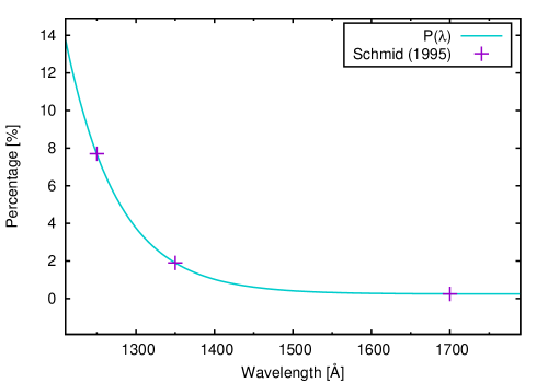
Figure 2: Percentage $P(\lambda)$ of the Rayleigh scattered photons in direction of the line of sight fitted to the data from the model S_B3 of Schmid (1995).

In the predominantly ionized region, the high photon flux from the hot components ($L_{\rm H}\approx 10^{2}-10^{4}$ $L_{\sun}$, Mürset et al. 1991; Greiner et al. 1997; Skopal 2005) produces free electrons by ionizing the neutral hydrogen in the RG’s wind. Column densities of the free electrons during quiescent phases of symbiotic stars, $n^{+}_{\rm e}\approx 10^{22}-10^{23}$ cm^-2  were determined by Sekeráš & Skopal (2012) assuming that the Thomson scattering is responsible for the broad wings of the strongest emission lines in the far-UV. Their values of $n^{+}_{\rm e}$ are consistent with our model based on H⁰ column density modelling (see below Eq. (9) and Fig. 6). Therefore, we suppose that the free electrons can be relevant for the attenuation of the stellar UV continuum by Thomson scattering. Further, the bound-free and free-free transitions on neutral hydrogen can be effective at a high electron temperature of nebula ($T_{\rm e}\approx 18500$ K, Skopal 2005).

Under these conditions, the optical depth through the ionized part of the wind can be written as,

$$\tau_{\lambda}^{+}(\varphi)=\sigma_{\rm e}n^{+}_{\rm e}(\varphi)+\sigma_{\rm H^{0}}(\lambda,\rm T_{e})n^{+}_{\rm H^{0}}(\varphi),$$ (8)

where $\sigma_{\rm e}$ is the Thomson scattering cross-section, $\sigma_{\rm H^{0}}(\lambda,\rm T_{e})$ the total cross-section of neutral hydrogen and $n^{+}_{\rm H^{0}}(\varphi)$ is the column density of H⁰ in the symbiotic nebula. We set the free electron column density

$$n^{+}_{\rm e}(\varphi)=1.2\,n^{+}_{\rm p}(\varphi),$$ (9)

where $n^{+}_{\rm p}(\varphi)$ is the column density of protons in the ionized area. The cross-section $\sigma_{\rm H^{0}}(\lambda,\rm T_{e})$ accounts for both bound-free and free-free transitions, i.e., $\sigma_{\rm H^{0}}(\lambda,\rm T_{e})=f_{\rm se}(\lambda,\rm T_{e})(\kappa_{\rm bf}(\rm H^{0})+\kappa_{\rm ff}(\rm H^{0}))$, where $\kappa_{\rm bf}(\rm H^{0})$ is the absorption coefficient for bound-free transitions and $\kappa_{\rm ff}(\rm H^{0})$ for free-free transitions of neutral hydrogen atom (e.g. Eq. (8.8) and (8.10) of Gray 2005, ; for the used values, see Table 2). The factor $f_{\rm se}$ accounts for the stimulated emission and $n^{+}_{\rm H^{0}}(\varphi)$ represents the variable in the LC modelling through the ionized wind region. In ionized region, the Thomson scattering and transitions of H⁰ have comparable attenuation effect on the WD radiation at $\lambda=1280$ Å, while the latter becomes dominant source of opacity with increasing wavelength (Fig. 1). In Sect. 5, we discuss the effect of other ions to the continuum attenuation.

Finally, we note that the description of the above-mentioned processes is valid in nebulae under conditions of the local thermodynamic equilibrium (LTE). This assumption is supported by the fact that the free electrons thermalize in nebulae very quickly, because of an extremely short time of their electrostatic encounters with respect to any other inelastic scatterings (see Bohm & Aller 1947). As a result, the energy distribution of free electrons can be characterized by a single $T_{\rm e}$. Modelling the UV/optical/near-IR spectral energy distribution (SED) during quiescent phases supports this assumption (see figures and Table 3 of Skopal 2005). However, e.g. Proga et al. (1998) used a non-LTE photoionization code to calculate the spectrum of a red giant wind illuminated by the hot component of a symbiotic binary. Therefore, the determination of H⁰ column density in ionized region can suffer from a systematic error in our simplified approach.

Table 2: Values of the Rayleigh scattering cross-section $\sigma_{\rm Ray}(\lambda)$ (in cm²), the percentage of the Rayleigh scattered photons in direction of the line of sight (in %), H^- bound-free absorption coefficient $\kappa_{\rm H^{-}}(\lambda)$ and total cross-section of neutral hydrogen $\sigma_{\rm H^{0}}(\lambda,\rm T_{e})$ at $\rm T_{e}=18500$ K (both in cm²) for 10 selected wavelengths.

$\lambda$ [Å]	$\sigma_{\rm Ray}(\lambda)$	$P(\lambda)$	$\kappa_{\rm H^{-}}(\lambda)$	$\sigma_{\rm H^{0}}(\lambda,\rm T_{e}$)
1280	$1.096\times 10^{-23}$	5.0	$4.56\times 10^{-18}$	$5.755\times 10^{-21}$
1340	$2.984\times 10^{-24}$	2.2	$4.85\times 10^{-18}$	$6.580\times 10^{-21}$
1450	$8.290\times 10^{-25}$	0.6	$5.51\times 10^{-18}$	$8.263\times 10^{-21}$
1520	$4.801\times 10^{-25}$	0.4	$5.81\times 10^{-18}$	$9.470\times 10^{-21}$
1600	$2.911\times 10^{-25}$	0.3	$6.20\times 10^{-18}$	$1.100\times 10^{-20}$
1800	$1.140\times 10^{-25}$	0.0	$7.31\times 10^{-18}$	$1.545\times 10^{-20}$
1950	$6.663\times 10^{-26}$	0.0	$8.07\times 10^{-18}$	$1.938\times 10^{-20}$
2400	$2.019\times 10^{-26}$	0.0	$1.10\times 10^{-17}$	$3.521\times 10^{-20}$
2700	$1.107\times 10^{-26}$	0.0	$1.31\times 10^{-17}$	$4.936\times 10^{-20}$
3080	$5.874\times 10^{-27}$	0.0	$1.58\times 10^{-17}$	$7.176\times 10^{-20}$

3.3 Column densities distribution

To calculate the total optical depth (Eq. (5)) along the line of sight to the WD, we need to determine functions $n_{\rm H^{0}}(\varphi)$ and $n^{+}_{\rm p}(\varphi)$. According to STB, we determine the ionization boundary by solving the parametric equation (see Nussbaumer & Vogel 1987),

$$X^{\rm H+}=f(u,\vartheta).$$ (10)

It defines the boundary between neutral and ionized hydrogen at the plane of observations by polar coordinates ($u,\vartheta$) with the origin at the hot star. The ionization parameter $X^{\rm H+}$ is expressed as

$$X^{\rm H+}=\frac{4\pi(\mu m_{\rm H})^{2}}{\alpha_{\rm B}({\rm H},T_{\rm e})}pL_{\rm ph}\left(\frac{v_{\infty}}{\dot{M}}\right)^{2},$$ (11)

where $\mu$ is the mean molecular weight, $m_{\rm H}$ the mass of the hydrogen atom, $\alpha_{\rm B}({\rm H},T_{\rm e})$ the total hydrogen recombination coefficient for recombinations other than to the ground state (Case B), $p$ the binary separation, $L_{\rm ph}$ the flux of ionizing photons from the WD, $v_{\infty}$ the terminal velocity of the wind from the giant and $\dot{M}$ its mass-loss rate.

Then, we can obtain the column density of neutral hydrogen by integrating H⁰ number density along the line of sight from the observer ($-\infty$) to the position of the ionization boundary $l_{\varphi}$,

$$n_{\rm H^{0}}(b)=\displaystyle\frac{a}{2}\displaystyle\int\limits_{-\infty}^{l_{\varphi}(b)}\displaystyle\frac{dl}{(l^{2}+b^{2})v(\sqrt{l^{2}+b^{2}})}.$$ (12)

where $a=\dot{M}/2\pi\mu m_{\rm H}$, $l$ is the coordinate along the line of sight, $b$ is the impact parameter (see Skopal & Shagatova 2012; Shagatova et al. 2016) and $v(\sqrt{l^{2}+b^{2}})$ is the wind velocity distribution (Sect. 3.4). The impact parameter represents the position of the binary through the orbital inclination $i$ and phase angle $\varphi$ as $b^{2}=p^{2}(\cos^{2}i+\sin^{2}\varphi\sin^{2}i)$. The value of the integral (12) decreases from the inferior conjunction of the RG and vanishes at the orbital phases, where the line of sight does not cross the H⁰ zone.

Similarly, we can obtain the column density of protons in the ionized area in the form,

$$n^{+}_{\rm p}(b)=\displaystyle\frac{a}{2}\displaystyle\int\limits_{-\infty/l_{\varphi}(b)}^{\pm\sqrt{p^{2}-b^{2}}}\displaystyle\frac{dl}{(l^{2}+b^{2})v(\sqrt{l^{2}+b^{2}})},$$ (13)

where the lower limit of integration is $l_{\varphi}(b)$ for orbital phases, at which the line of sight passes through the neutral area, and $-\infty$ outside it. The sign plus in the upper limit of integration (i.e. the position of the WD) applies for values of the angle between the line of sight and the line connecting the binary components, $\vartheta\in\langle-\pi/2,\pi/2\rangle$, and the sign minus applies for $\vartheta\in\langle-\pi,-\pi/2\rangle\cup\langle\pi/2,\pi\rangle$.

For the orbital phases during the eclipse, i.e. for $b\leq R_{\rm g}$ (= the radius of the RG), we integrated $n_{\rm H^{0}}(b)$ up to the giant surface, i.e. $l=-\sqrt{R_{\rm g}^{2}-b^{2}}$, and put $n^{+}_{\rm p}(b)=0$.

3.4 Velocity profiles

3.4.1 Components derived from observations

The functions for the column densities of neutral and ionized hydrogen (Eq. (12) and (13)) are determined by the wind velocity distribution. We adopt the velocity profiles from Shagatova et al. (2016), derived by modelling the H⁰ column densities, measured from the Rayleigh attenuation around the Ly-$\alpha$ line during ingress and egress orbital phases, using the inversion method of Knill et al. (1993) and the ionization structure model STB. We use their egress model M and ingress model O, denoting them here as $v_{\rm e}(r)$ and $v_{\rm in}(r)$:

$$v_{\rm in}(r)=\displaystyle\frac{v_{\rm in\,\infty}}{1+1.81\times 10^{4}\displaystyle\left(\frac{r}{R_{\rm g}}\right)^{-12}}$$ (14)

and

$$v_{\rm e}(r)=\displaystyle\frac{v_{\rm e\,\infty}}{1+2.94\times 10^{3}\displaystyle\left(\frac{r}{R_{\rm g}}\right)^{-7}},$$ (15)

where $v_{\rm in\,\infty}$ and $v_{\rm e\,\infty}$ are corresponding terminal velocities of the wind. The ingress velocity profile is steeper than the egress profile, thus, it indicates an asymmetric wind distribution at the plane of observations. For eclipsing binaries, the plane of observations roughly coincides with the orbital plane.

For the egress terminal velocity we adopted $v_{\rm e\infty}=20$ km s^-1, which is within a typical range of the terminal velocities of symbiotic stars (e.g. Dumm et al. 1999; Schmid et al. 1999). The selected value of $v_{\rm e\infty}$ yields $\dot{M}$ of the model, using Eq. (18) of Shagatova et al. (2016). However, this value represents the spherical equivalent of the mass-loss rate because of the asymmetry in the wind distribution around the RG.

3.4.2 Model of a complete velocity profile

As we aim to model the continuum LCs of SY Mus for the complete range of phases, we need to propose a unified model of the velocity profile by interconnecting $v_{\rm in}(r)$ and $v_{\rm e}(r)$ components around the orbital phase $0$, where the observations of column densities are not available; i.e. for the so-called transition area. We assume that the velocity profile changes gradually in a smooth way from $v_{\rm in}(r)$ to $v_{\rm e}(r)$ at the plane of observations, i. e. we are looking for the transition velocity profile, $v_{\rm trans}(r,\psi)$, where $\psi$ is the azimuth angle at the plane of observations in the coordinate system centered at the RG. Thus, the $v_{\rm trans}(r,\psi)$ function is defined for $\psi\in\langle\psi_{\rm in},\psi_{\rm e}\rangle$, where angles $\psi_{\rm in}$ and $\psi_{\rm e}$ bound the transition area. In determining the $v_{\rm trans}(r,\psi)$ function, we require the following conditions:

• the unified function for the velocity profile has to be a smooth (C¹) function of $\psi$,

• corresponding functions, $n_{\rm H^{0}}(\varphi)$, $n^{+}_{\rm p}(\varphi)$, and the position of the ionization boundary, $l_{\varphi}$, have to be smooth (C¹) functions of $\varphi$,

• unified model of $n_{\rm H^{0}}(\varphi)$ has to fit the observed H⁰ column densities.

The transition velocity profile affects the model density distribution of the wind mainly at the area corresponding to the lines of sight during the eclipse.

Since a linear function of $\psi$ cannot meet the conditions for $v_{\rm trans}(r,\psi)$, we assume the transition velocity profile in the form:

$$v_{\rm trans}(r,\psi)=v_{\rm in}(r)\cos^{2}(C_{\rm in}\psi+D_{\rm in})+v_{\rm e}(r)\cos^{2}(C_{\rm e}\psi+D_{\rm e}),$$ (16)

where $C_{\rm in}$, $D_{\rm in}$, $C_{\rm e}$ and $D_{\rm e}$ are parameters. We divided the complete range of $\psi$, from $0$ to $2\pi$, into 4 areas with different velocity profiles, as depicted in Fig. 3. In front of the RG along the orbital motion, there is an area, where the $v_{\rm e}(r)$ profile applies. At the opposite side, the $v_{\rm in}(r)$ profile is implemented. Finally, there are two more zones in between, where the transitional velocity profile applies.

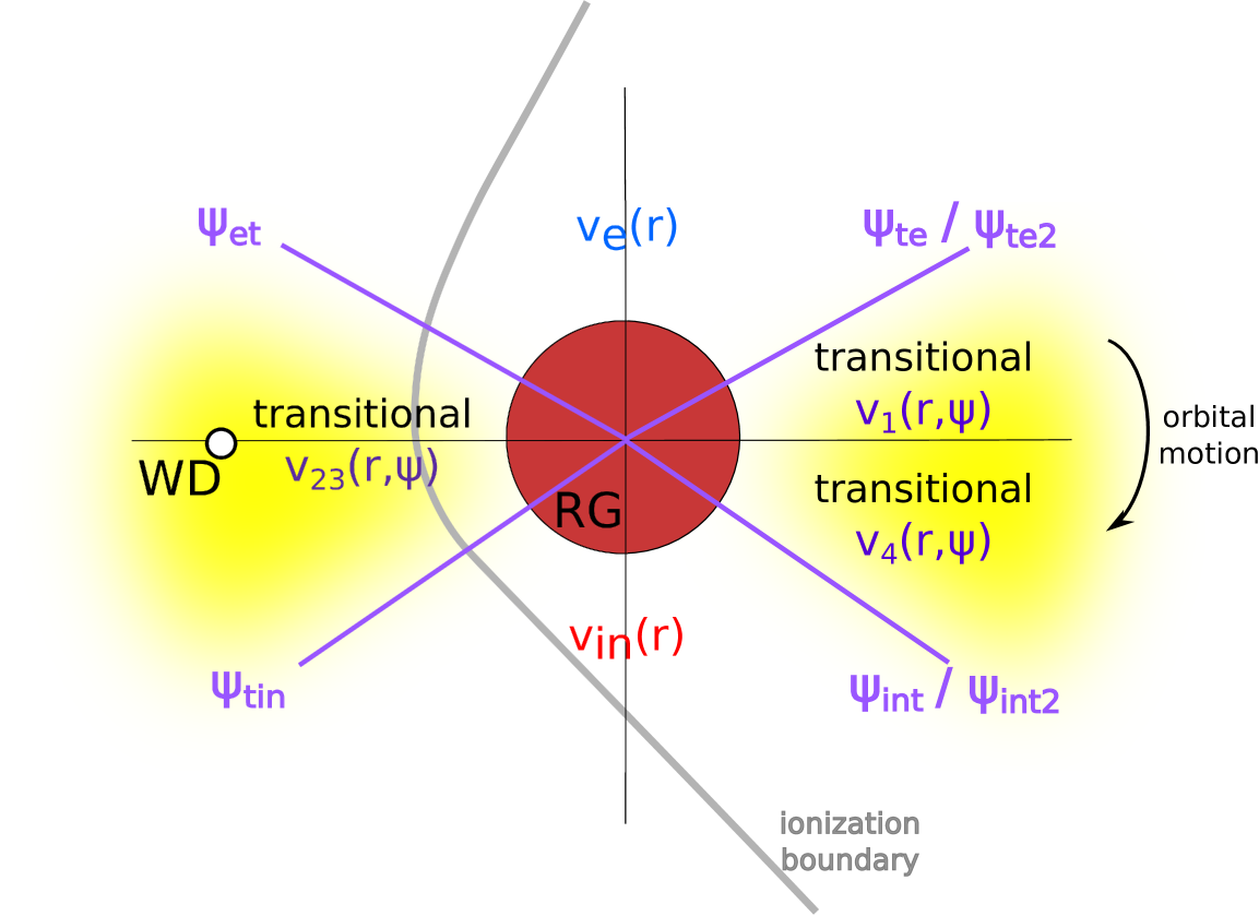
Figure 3: Schematic view of the regions of different velocity profiles as seen perpendicularly to the plane of observations. Denotations are explained in Sect. 3.4.

From the computational point of view, the $v_{\rm trans}(r,\psi)$ profile is defined by three functions: $v_{1}(r)$, $v_{23}(r)$ and $v_{4}(r)$. The interconnection of $v_{\rm in}(r)$ and $v_{\rm e}(r)$ from the quadrant II to III of the values of $\psi$ is given by $v_{23}(r)$, the interconnection between the quadrant I and IV is given by two functions, $v_{1}(r)$ and $v_{4}(r)$, because of the discontinuity in values of $\psi$ around $\psi=0=2\pi$. The axisymmetric boundaries of $v_{\rm e}(r)$ and $v_{\rm in}(r)$ regions are given by relations between limiting values of $\psi$ (see Fig. 3):

$\psi_{\rm te}\in\langle 0,\pi/2\rangle,\hskip 55.48277pt\psi_{\rm int}\in\langle-\pi/2,0\rangle$,

$\psi_{\rm et}=\pi-\psi_{\rm te},\hskip 58.32823pt\psi_{\rm tin}=\pi-\psi_{\rm int}$,

$$\psi_{\rm te2}=2\pi+\psi_{\rm te},\vspace{3.0mm}\hskip 49.79231pt\psi_{\rm int2}=2\pi+\psi_{\rm int},$$ (17)

where the subscript ”te” denotes the boundary from transitional to egress velocity profile area and ”et” the boundary for the transition in the opposite direction, in the direction of increasing values of $\psi$. Similarly, the subscript ”int” denotes the boundary from ingress to transitional zone and ”tin” from the transitional to ingress zone. Then, from the conditions of smoothness of the united velocity profile (i.e. the first derivative of the corresponding function has to be continuous for C¹ function), we obtain the formulae for velocity profiles defining $v_{\rm trans}(r,\psi)$:

$$v_{1}(r,\psi)=v_{\rm in}(r)\cos^{2}[C(\psi-\psi_{\rm int})]+v_{\rm e}(r)\cos^{2}[C(\psi-\psi_{\rm te})],$$ (18)

$$v_{23}(r,\psi)=v_{\rm in}(r)\cos^{2}[C(\psi_{\rm tin}-\psi)]+v_{\rm e}(r)\cos^{2}[C(\psi-\psi_{\rm et})],$$ (19)

$$v_{4}(r,\psi)=v_{\rm in}(r)\cos^{2}[C(\psi_{\rm int2}-\psi)]+v_{\rm e}(r)\cos^{2}[C(\psi-\psi_{\rm te2})],$$ (20)

where $C=\dfrac{\pi}{2(\psi_{\rm int}-\psi_{\rm te})}$, and corresponding transitional terminal velocities ($r\rightarrow\infty$) are:

$$v_{1\,\infty}(\psi)=v_{\rm in\,\infty}\cos^{2}[C(\psi-\psi_{\rm int})]+v_{\rm e\,\infty}\cos^{2}[C(\psi-\psi_{\rm te})],$$ (21)

$$v_{23\,\infty}(\psi)=v_{\rm in\,\infty}\cos^{2}[C(\psi_{\rm tin}-\psi)]+v_{\rm e\,\infty}\cos^{2}[C(\psi-\psi_{\rm et})],$$ (22)

$$v_{4\,\infty}(\psi)=v_{\rm in\,\infty}\cos^{2}[C(\psi_{\rm int2}-\psi)]+v_{\rm e\,\infty}\cos^{2}[C(\psi-\psi_{\rm te2})].$$ (23)

Equations (18) – (20) and also powers of their right sides to the $-1$ and $-2$, which are present in formulae for the position of the ionization boundary (Eq. (8) of Nussbaumer & Vogel (1987)) and column density (Eq. (12) and (13)) fulfill the conditions of smoothness. The last condition for $v_{\rm trans}(r,\psi)$, i. e. the correctness of fits to the observed H⁰ column densities, is linked with the selection of the values of $\psi_{\rm te}$ and $\psi_{\rm int}$ (see Sect. 3.5 and 4).

3.5 Ionization parameter

To determine the position of the ionization boundary $l_{\varphi}$, values of the ionization parameter $X^{\rm H+}$ are needed. Similarly as in the previous section, we adopt them from the column density models M and O of Shagatova et al. (2016), i. e., we have $X^{\rm H+}_{\rm in}=16$ before the eclipse and $X^{\rm H+}_{\rm e}=2.5$ after it. Therefore, using Eqs. (11) and (21) – (23), we obtain the formulae for the transitional ionization parameters:

$$X^{\rm H+}_{1}(\psi) = X^{\rm H+}_{\rm in}\cos^{4}[C(\psi-\psi_{\rm int})]$$

$$+2\sqrt{X^{\rm H+}_{\rm in}X^{\rm H+}_{\rm e}}\cos^{2}[C(\psi-\psi_{\rm int})]\cos^{2}[C(\psi-\psi_{\rm te})]$$

$$+X^{\rm H+}_{\rm e}\cos^{4}[C(\psi-\psi_{\rm te})],$$

$$X^{\rm H+}_{23}(\psi) = X^{\rm H+}_{\rm in}\cos^{4}[C(\psi_{\rm tin}-\psi)]$$

$$+2\sqrt{X^{\rm H+}_{\rm in}X^{\rm H+}_{\rm e}}\cos^{2}[C(\psi_{\rm tin}-\psi)]\cos^{2}[C(\psi-\psi_{\rm et})]$$

$$+X^{\rm H+}_{\rm e}\cos^{4}[C(\psi-\psi_{\rm et})],$$

$$X^{\rm H+}_{4}(\psi) = X^{\rm H+}_{\rm in}\cos^{4}[C(\psi_{\rm int2}-\psi)]$$

$$+2\sqrt{X^{\rm H+}_{\rm in}X^{\rm H+}_{\rm e}}\cos^{2}[C(\psi_{\rm int2}-\psi)]\cos^{2}[C(\psi-\psi_{\rm te2})]$$

$$+X^{\rm H+}_{\rm e}\cos^{4}[C(\psi-\psi_{\rm te2})],$$

with the subscript notation equivalent to the previous section.

Further, under the assumption of spherically symmetric mass flux at $r\rightarrow\infty$, we can put into equality the expression for $\dot{M}$ from Eq. (11) for ingress values of variables with that from the same equation for egress values of variables to obtain a relation,

$$\dfrac{X^{\rm H+}_{\rm in}}{X^{\rm H+}_{\rm e}}=\dfrac{v_{\rm in\,\infty}^{2}}{v_{\rm e\,\infty}^{2}}$$ (27)

and, then, by evaluating egress and ingress ionization parameters, we obtain a relation between terminal velocities before and after the eclipse,

$$v_{\rm in\,\infty}=2,53v_{\rm e\,\infty}.$$ (28)

This equation reflects the simple distribution of ionization parameter values (3.5) - (3.5) at the orbital plane and the fact that values of $X^{\rm H+}_{\rm in}$ and $X^{\rm H+}_{\rm e}$ were determined by fitting $n^{\rm obs}_{\rm H^{0}}$ values only at the area close to RG (Fig.6). Since the derivation of Eq. (28) is based on the equal mass-loss in front and behind the RG with respect to its orbital motion, the difference in corresponding hydrogen densities in radial directions results from the different velocity profiles (14) and (15).

The selection of values of $\psi_{\rm int}$ and $\psi_{\rm te}$ has to satisfy several conditions. First, it has to preserve the correctness of the M and O column density models of Shagatova et al. (2016). At the same time, the range of the angle $\psi$, where the transitional velocity profile and ionization parameter apply, has to be sufficiently wide to prevent the corresponding interconnection between the ingress and egress ionization boundary to be too sharp.

4 The results

In this section, we use Eqs. (2) - (28) to model the asymmetric UV continuum LCs obtained from low-resolution IUE spectra (Table 1). Main results may be summarized as follows:

(i) We determined the ionization structure by solving Eq. (10) with the united velocity profile (18) - (20) and the corresponding ionization parameter (3.5) - (3.5). The resulting shape of the ionization boundary is depicted in Fig. 4.

(ii) Comparing the wind velocity profiles $v_{\rm in}(r)$ and $v_{\rm e}(r)$ (Fig. 5), the ingress wind velocity is lower than the egress velocity at the distance up to $\approx 1$ R_g from the RG surface. It implies a higher hydrogen number density of the wind in front of the RG than behind it, in the direction of the orbital motion. On the other hand, at larger distances, the wind velocity and thus, the wind number density proportion is opposite. The asymmetry of the ionization boundary in Fig. 4 is in agreement with this fact.

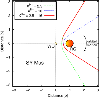
Figure 4: Resulting ionization boundary for the united wind velocity model given by Eqs. (14), (15) and (18) – (28), as seen perpendicularly to the orbital plane (solid line). The corresponding limiting values of $\psi$ are $\psi_{\rm int}=-0.9$ rad and $\psi_{\rm te}=0.8$ rad. For comparison, dotted line represents the ionization boundary for $X^{\rm H+}=X_{\rm in}^{\rm H+}$ and $v(r)=v_{\rm in}(r)$, whereas dashed line for $X^{\rm H+}=X_{\rm e}^{\rm H+}$ and $v(r)=v_{\rm e}(r)$.

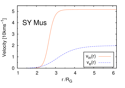
Figure 5: Ingress and egress velocity profiles of SY Mus from models M and O of Shagatova et al. (2016) for $v_{\rm e\infty}=20$ km s^-1 satisfying Eq. (28).

(iii) We determined values of $n_{\rm H^{0}}(b)$ and $n^{+}_{\rm p}(b)$ functions for the unified model of the velocity profile and ionization structure according to Eqs. (12) and (13), using $R_{\rm g}$ as the length unit. Their sum provides the total hydrogen column density $n_{\rm H}$ (see Fig. 6).

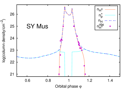
Figure 6: United column density model, $n_{\rm H}$ and its components, $n_{\rm H^{0}}$ and $n^{+}_{\rm p}$; $n^{\rm obs}_{\rm H^{0}}$ are the measured column densities of the neutral hydrogen from Dumm et al. (1999). During the eclipse, column densities are computed from the observer to the surface of the RG.

(iv) Finally, we modelled the continuum fluxes of SY Mus (Table 1) using Eq. (4). The resulting models are depicted in Fig. 7. Corresponding contributions from the nebula and a comparison with the values from the model SED at $\varphi=0.62$ is in Fig. 8. The model SED suggests a slightly more rapid increase of the continuum nebular flux with wavelength than the LC model. However, parameters of the nebular contribution are subject to variation from cycle to cycle (Skopal 2005). The modelling yielded column densities $n_{\rm H^{-}}(\varphi)=5.0\times 10^{-7}n_{\rm H^{0}}(\varphi)$ and $n^{+}_{\rm H^{0}}(\varphi)=1.5\times 10^{-4}n^{+}_{\rm p}(\varphi)$. We estimated their uncertainties by the LC models for $\lambda=1450$ Å  and $\lambda=1950$ Å, respectively (see Fig. 9). Corresponding values of $n_{\rm H^{-}}$ and $n^{+}_{\rm H^{0}}$ are consistently used in all 10 LC models, from $\lambda=1280$ Å  to $\lambda=3080$ Å.

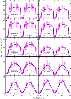
Figure 7: LCs of SY Mus (circles with errorbars) and their models (solid lines). Contribution from the nebula is depicted by dashed lines. Vertical dotted lines represent the position of the inferior conjunction of the giant.

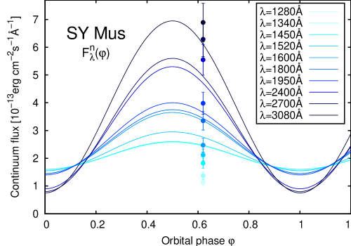
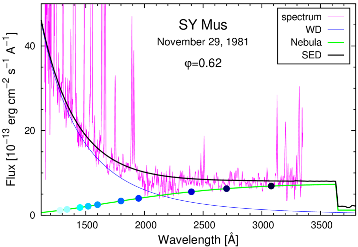
Figure 8: Top: The model variations of the nebular continuum radiation in SY Mus (Eq. 3) at 10 wavelengths (solid lines). They are compared with the nebular fluxes at $\varphi=0.62$ from the model SED (circles with errorbars). Bottom: The model SED of SY Mus at $\varphi=0.62$. Circles at the nebular component correspond to those plotted at the top panel.

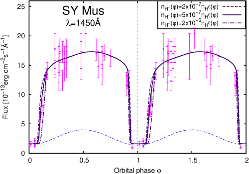
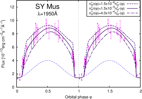
Figure 9: Representative LC models for different column densities $n_{\rm H^{-}}(\varphi)$ (top) and $n^{+}_{\rm H^{0}}(\varphi)$ (bottom).

5 Discussion

Results of our analysis are limited by simplifying assumptions and quality of the data. Basic assumption we made is that the wind from the giant is composed solely by the hydrogen in different states/forms and that it flows radially. Further, we neglected an influence of the hot component wind, because it is a factor of $\approx 10$ weaker than that from the RG during quiescent phases (Skopal 2006). As the real composition and the flow of the wind is more complex, these assumptions represent sources of systematic errors.

Further simplification is given by the selection of sources attenuating the continuum radiation, i. e. H⁰ atoms, H^- ions and free electrons. We tested the sensitivity of our LC model on the value of product of the column density and the continuum cross-section of atom/ion X, $n_{\rm X}\sigma_{\rm X}$. We have found no detectable attenuation effect to the LC for $n_{\rm X}\sigma_{\rm X}/n^{+}_{\rm p}\lesssim 10^{-26}$ cm² in the ionized region and for $n_{\rm X}\sigma_{\rm X}/n_{\rm H^{0}}\lesssim 10^{-29}$ cm² in the neutral region. Using these relations, we checked, whether H${}_{2}^{+}$ and H^- ions as other possible sources of scattering the continuum can contribute to the LC attenuation in the ionized region. We found that none of them has a measurable effect for the column density values from the model for symbiotic stars of Schwank et al. (1997) or even higher values of column density according to the model for planetary nebulae of Aleman & Gruenwald (2004). Also the concentrations of free electrons and protons in neutral area are too low (Schwank et al. 1997; Crowley 2006) to have a recognizable effect on the continuum UV radiation. However, due to the simplifications in our model, we cannot exclude the effect of other species than those included in our model and, therefore, we consider the resulting functions $n^{+}_{\rm H^{0}}(\varphi)$ and $n_{\rm H^{-}}(\varphi)$ as the upper limits estimate of the column densities of H⁰ atoms in the ionized region and H^- ions in the neutral region.

In determining column densities $n_{\rm H^{-}}(\varphi)$ and $n^{+}_{\rm H^{0}}(\varphi)$, we preliminary approximated these functions using expressions that qualitatively correspond to the $n_{\rm H^{-}}/n_{\rm H^{0}}$ and $n^{+}_{\rm H^{0}}/n^{+}_{\rm p}$ profiles of Aleman & Gruenwald (2004) for planetary nebulae. However, these expressions and their modifications did not represent observed fluxes near to the eclipse. Therefore, H^- and H⁰ densities probably rapidly change at the ionization boundary, as in the models for H⁰ and H⁺ populations of Schwank et al. (1997). Thus, we simply used linear functions of the column density of the corresponding prevalent form of the hydrogen (Sect. 4, point (v)). Therefore, functions $n_{\rm H^{-}}(\varphi)$, $n^{+}_{\rm H^{0}}(\varphi)$ and $n^{+}_{\rm e}(\varphi)$ depend on $n_{\rm H^{0}}(\varphi)$ or $n^{+}_{\rm p}(\varphi)$ that are given by velocity profiles derived from observations.

A large scatter in the observed fluxes (Fig. 7) does not allow to determine the nebular continuum variations, $F^{\rm n}_{\lambda}(\varphi)$, accurately. To put a constraint on the resulting nebular component, we required a monotone increasing of the nebular flux with wavelength for $\varphi\approx 0.5$ and its monotone decreasing for $\varphi\approx 1$, as in the models SED (Skopal 2009). Figure 8 shows an example of the model SED at the orbital phase $\varphi=0.62$ and a comparison of its $F^{\rm n}_{\lambda}(0.62)$ fluxes with those from our LC models. Both models are roughly consistent. However, dependence of our model nebular flux on the wavelength is not monotone for $\varphi\approx 0.1$ and $0.9$ due to the worse quality of the data.

Further simplification is given by the approximation that the nebular continuum varies with the orbital phase as a sine function (Eq. (3)). Since during quiescent phases the symbiotic nebula represents the ionized fraction of the wind from the giant, the asymmetric wind distribution will produce a nebula, which is asymmetric with respect to the binary axis and thus its flux. However, with given uncertainties in the data, this effect is not recognizable even for LCs with dominant nebular contribution, for $\lambda>2000$ Å (Fig.7). Comparing our resulting nebular fluxes with those of Skopal (2005) and Skopal (2009) from models SED at $\varphi=0.02$ and $\varphi=0.62$, we found different values by a factor $1.04-1.89$, which is given by the scatter of the data at a given wavelength (also Fig. 8).

Furthermore, we considered a continuous change of the velocity profile within the transition region (Eq. (16)), which affects mainly the profiles around maxima and minima of the model LCs. Applicability of our transition velocity profile is supported by the resulting LC models that describe the eclipse profiles of the observed LCs. Particularly, a good match was found for the LC at $\lambda=2700$ Å  (the reduced $\chi$-squared $\chi^{2}_{\rm red}=0.4$). Overall, the values of $\chi^{2}_{\rm red}$ of our models varies from the order of $0.1$ to the order of $10$.

To improve the presented modelling, better quality spectra of the symbiotic systems are needed, preferably in such quantity that even single orbital cycle can be covered sufficiently, to avoid physical changes of the particular system with time. With this kind of data, refinement of the model parameters would be possible and also including the asymmetric nebula model would be meaningful.

An independent way how to probe the asymmetric distribution of the circumstellar matter in symbiotic binaries from observations, as suggested by our continuum analysis (Shagatova et al. 2016, and this paper), is to investigate dramatic and strictly orbitally-related variation of the H$\alpha$ line profile observed in the spectra of other quiet symbiotic stars. The main goal is to model the orbital variations of both the absorption and emission component in the H$\alpha$ line profile as a function of the orbital phase, using our column density model. This means to investigate the absorbing/scattering layer of the neutral wind from above the RG photosphere and the line emitting H⁺ region, with the aim to determine the H$\alpha$ line profile at each orbital phase. And in this way, to obtain the corresponding velocity profile of the circumstellar matter, its distribution with respect to the binary axis and the spherical equivalent of the mass-loss rate. Solving this task should also provide constraints for further theoretical modelling of the RG wind in symbiotic binaries, its transfer to and accretion onto the compact companion.

6 Conclusion

We modelled the IUE continuum fluxes of the eclipsing symbiotic system SY Mus at 10 wavelengths from $1280$ to $3080$ Å  (Table 1, available online). To evaluate attenuation of the WD radiation passing the wind from the RG at different wavelengths and orbital phases, we considered the Rayleigh scattering on neutral hydrogen atoms and the bound-free absorption by negative hydrogen ion in the neutral wind region, and the Thomson scattering on free electrons and the bound-free and free-free transitions on the neutral hydrogen atom in the ionized region (Eqs. 6 and 8).

To obtain the column densities of relevant forms of hydrogen at all orbital phases, we used the asymmetric wind velocity profile (Sect. 3.4) and the corresponding ionization boundary model (Fig. 4). Accordingly, we obtained the column density distribution of H⁰ in the neutral region and H⁺ in the ionized region (Fig. 6). From the shape of the observed LCs, we obtained the distribution of the H^- column density $n_{\rm H^{-}}(\varphi)/n_{\rm H^{0}}(\varphi)=5.0\times 10^{-7}$ that can be considered as the upper limit due to the simplifications in the model (Sect. 4, Fig. 9). Resulting LC models of SY Mus (Eq. (4), Fig. 7) match well the asymmetric shape of the observed flux profiles. The nebular contribution was approximated by a sine waves (Sect. 4, Fig. 8).

This paper presents the first quantitative model of the UV LCs of the S-type symbiotic star. We found that the different shapes of descending and ascending parts of the observed UV continuum LCs of SY Mus are caused by the asymmetric distribution of the wind from the RG at the near-orbital region.