Generalized two-field $\alpha$-attractor models from the hyperbolic triply-punctured sphere

Abstract

We study generalized two-field $\alpha$-attractor models whose rescaled scalar manifold is the triply-punctured sphere endowed with its complete hyperbolic metric, whose underlying complex manifold is the modular curve $Y(2)$. Using an explicit embedding into the end compactification, we compute solutions of the cosmological evolution equations for a few globally well-behaved scalar potentials, displaying particular trajectories with inflationary behavior as well as more general cosmological trajectories of surprising complexity. In such models, the orientation-preserving isometry group of the scalar manifold is isomorphic with the permutation group on three elements, acting on $Y(2)$ as the group of anharmonic transformations. When the scalar potential is preserved by this action, $\alpha$-attractor models of this type provide a geometric description of two-field “modular invariant $j$-models” in terms of gravity coupled to a non-linear sigma model with topologically non-trivial target and with a finite (as opposed to discrete but infinite) group of symmetries. The precise relation between the two perspectives is provided by the elliptic modular function $\lambda$, which can be viewed as a field redefinition that eliminates almost all of the countably infinite unphysical ambiguity present in the Poincaré half-plane description of such models.

Introduction

Reference genalpha introduced a very large class of two-field cosmological models called generalized two-field $\alpha$-attractors. These form a tractable sub-family of the extremely wide class of two-field cosmological models, which – along with general multi-field models – are a subject of active theoretical interest (see, for example, PT1 ; PT2 ; m1 ; m2 ; m3 ; m4 ; m5 ; m6 ; Sch01 ; Sch02 ; Sch1 ; Sch2 ; Gong ; Dias1 ; Dias2 ; Mulryne ; c1 ; BBJMV ). Indeed, multi-field models are easier to produce than one field models in fundamental theories of gravity and future observations at higher precision that current data Planck (which at present are well accounted for by one-field models) may allow one to detect multi-field effects in the future.

Generalized two-field $\alpha$-attractors are derived from four-dimensional gravity coupled to a non-linear sigma model whose scalar manifold $\Sigma$ is a borderless, connected, oriented and non-compact smooth surface, endowed with a complete metric ${\mathcal{G}}$ of constant negative curvature, with a scalar potential given by a smooth real-valued function $\Phi$ defined on $\Sigma$. The cosmological models derived from such a theory provide a wide generalization of the two-field version of ordinary $\alpha$-attractors alpha5 ; Escher (for which $(\Sigma,{\mathcal{G}})$ is – up to a constant rescaling of the metric – given by the hyperbolic disk). In a naive one-field truncation, such generalized models have the same universal behavior as one-field $\alpha$-attractors alpha3 ; alpha4 for those special trajectories for which the fields undergo slow motion along geodesics flowing from an end of $\Sigma$ where the scalar potential is “well-behaved” and “locally maximal” toward the compact core of $\Sigma$ (see genalpha for details). This property justifies the name ‘generalized two-field $\alpha$-attractors’ which was given in genalpha to such models. The role of the parameter $\alpha$ is played by the quantity $\frac{1}{3|K|}$, where $K<0$ is the Gaussian curvature of ${\mathcal{G}}$. Equivalently, we have ${\mathcal{G}}=3\alpha G$, where $G$ is a complete hyperbolic metric on $\Sigma$, i.e. a complete metric of constant Gaussian curvature equal to $-1$. As shown in genalpha , such models can be studied using uniformization theory (see unif ; Katok ; Beardon ; FN for an introduction). They allow for multipath inflation when the scalar potential or the topology of $\Sigma$ are sufficiently nontrivial and they have intricate cosmological dynamics already when $(\Sigma,G)$ is an elementary hyperbolic surface elem . We shall freely use certain results and notions from the geometry of hyperbolic surfaces, which we summarized in (genalpha, , Appendices B,C,D) for the convenience of cosmologists. We refer the reader to loc. cit. for relevant information. As explained in the present paper, those special two-field generalized $\alpha$-attractors for which the underlying complex manifold of $(\Sigma,G)$ is a modular curve can be related through uniformization to the modular-invariant cosmological models considered in Sch01 ; Sch1 ; Sch2 . The reader should notice that the underlying complex curve of a hyperbolic surface $(\Sigma,G)$ of a generalized two-field $\alpha$-attractor model need not be a modular curve. Indeed, such a hyperbolic surface may have infinite area and may have ends whose hyperbolic type is not that of a cusp end. The simplest such examples are provided by the elementary hyperbolic surfaces (namely the hyperbolic disk, hyperbolic punctured disk and hyperbolic annuli), which were considered in detail in reference elem . Even for the simple case of “modular $j$-inflation” (which was considered in Sch1 ; Sch2 ), the relation to two-field generalized $\alpha$-attractors is somewhat subtle, as we explain in the present paper.

In this paper, we consider the case when $\Sigma$ is the triply-punctured sphere (equivalently, the doubly-punctured complex plane) endowed with its unique complete hyperbolic metric $G$. With respect to this metric, the three punctures of the sphere are located at infinite distance from the compact core, determining three hyperbolic cusp regions Borthwick of infinite length but finite area. The hyperbolic area of the triply-punctured sphere is finite and equals $2\pi$. Such a surface can be viewed as a degeneration of a hyperbolic pair of pants, in the limit when each of the cuff lengths of the latter tends to zero. When viewed as a smooth non-compact complex (or affine algebraic) curve, the hyperbolic triply-punctured sphere coincides with one of the classical non-compact modular curves DS ; Shimura , usually denoted by $Y(2)$. It is uniformized by a non-Abelian surface group $\Gamma(2)\subset\mathrm{PSL}(2,\mathbb{Z})$ which is freely generated by two parabolic elements, namely the principal congruence subgroup of $\mathrm{PSL}(2,\mathbb{Z})$ at level two. The uniformization map from the Poincaré half-plane is given Ahlfors by the classical elliptic modular function $\lambda$.

The end (a.k.a. Kerékjártó-Stoilow) compactification of $Y(2)$ is the unit sphere $\mathrm{S}^{2}$. The conformal compactification (which in this case is usually denoted by $X(2)$) is the unit sphere endowed with its unique orientation-compatible complex structure, i.e. the Riemann sphere $\mathbb{C}\mathbb{P}^{1}$. An explicit embedding of $Y(2)$ into the Riemann sphere is obtained by restricting the inverse of the stereographic projection. A smooth scalar potential defined on $Y(2)$ is globally well-behaved in the sense of genalpha iff it is induced through this projection by a smooth real-valued map $\hat{\Phi}$ defined on the sphere. Using these observations, one can describe globally well-behaved scalar potentials defined on $Y(2)$ by expanding $\hat{\Phi}$ into spherical harmonics.

As explained in genalpha , cosmological trajectories of the generalized $\alpha$-attractor model defined by $Y(2)$ can be obtained by first computing trajectories of an appropriately lifted model defined on the Poincaré half-plane and then projecting the latter to $Y(2)$ through the uniformization map. Using this method, we compute cosmological trajectories for a few globally well-behaved scalar potentials. In particular, we display trajectories which have inflationary behavior for small enough times. We find that the model exhibits rich cosmological dynamics already in the absence of a scalar potential, which becomes even more complex when the scalar potential is included. We also find inflationary trajectories which produce between 50 and 60 efolds, thus showing that such models are potentially relevant to observational cosmology.

The lift genalpha of the two-field generalized $\alpha$-attractor models based on $Y(2)$ to the Poincaré half-plane can be viewed as modular-invariant cosmological models in the sense of Sch1 ; Sch2 for the modular group $\Gamma(2)$. The description provided by the lifted model, while convenient for some purposes, contains a countably infinite ambiguity which signals the fact that the physically-relevant scalar field is not valued in the Poincaré half-plane but in the triply-punctured sphere $Y(2)$. The uniformization map $\lambda$ can be viewed as a (countable to one) field redefinition which eliminates this unphysical ambiguity, thus affording easier understanding of the physics near the cusp ends of $Y(2)$.

The orientation-preserving isometry group of the hyperbolic triply-punctured sphere is isomorphic with the permutation group on three elements, acting on $Y(2)$ as the anharmonic subgroup $\mathfrak{B}$ of $\mathrm{PSL}(2,\mathbb{C})$, which permutes the three punctures. The triply-punctured sphere can be written as a six-fold branched cover $q:Y(2)\rightarrow\mathbb{C}$ of the complex plane in such a way that the composition $q\circ\lambda$ coincides with the modular $j$ function. The anharmonic action permutes the branches of this cover, hence the topological quotient $Y(2)/\mathfrak{B}$ can be identified with the complex plane. Since $q$ is ramified above two points of the complex plane, the hyperbolic metric of $Y(2)$ descends to a singular metric on the topological quotient $\mathbb{C}=Y(2)/\mathfrak{B}$. When the scalar potential $\Phi$ is preserved by the anharmonic action, the generalized $\alpha$-attractor model with scalar manifold $Y(2)$ has an $S_{3}$ symmetry and the corresponding lifted model is a “$j$-model” in the sense of Sch1 ; Sch2 , being invariant under the entire classical modular group $\mathrm{PSL}(2,\mathbb{Z})$. In that case, the field redefinition provided by the elliptic modular function $\lambda$ eliminates an infinite $\Gamma(2)$-ambiguity, replacing it with a finite $\mathfrak{B}\simeq S_{3}$ symmetry. The latter cannot be eliminated directly within the framework of generalized two-field $\alpha$-attractor models, since taking the quotient through the anharmonic action of $S_{3}$ would lead to a singular metric on the complex plane, which is disallowed in the usual construction of non-linear sigma models by the principle of conservation of energy.

The paper is organized as follows. Section 1 briefly recalls the definition of generalized $\alpha$-attractor models and the lift of their cosmological equations of motion to the Poincaré half-plane. It also explains when the lift to the Poincaré half-plane can be interpreted as a modular-invariant cosmological model in the sense of Sch01 ; Sch1 ; Sch2 and discusses symmetries of such models. In section 2, we describe the end and conformal compactifications as well as the hyperbolic geometry of $Y(2)$, its symmetries and its uniformization. We also explain the difference between $Y(2)$ (which coincides with the coarse moduli space of elliptic curves with level $2$ structure) and the usual coarse moduli space of elliptic curves (which equals the complex plane), of which $Y(2)$ is a branched six-fold cover. This accounts for the difference between the elliptic modular functions $\lambda$ and $j$, which differ by composition with a rational function. This is standard mathematical material which we chose to explain in some detail since it may be unfamiliar to cosmologists. Finally, we show that modular-invariant cosmological models for the classical modular group $\mathrm{PSL}(2,\mathbb{Z})$ (see Sch1 ; Sch2 ) are related by a countable to one field redefinition to those generalized two-field $\alpha$-attractor models with scalar manifold $Y(2)$ for which the scalar potential is invariant under the action of the anharmonic group. Section 3 discusses globally well-behaved scalar potentials on the triply-punctured sphere and presents examples of numerically-computed cosmological trajectories. In particular, we present examples of inflationary trajectories which produce between 50 and 60 efolds. In Section 4, we discuss the gradient flow approximation near cusp ends and a class of scalar potentials for which one can obtain any desired number of efolds for certain ‘universal’ cosmological trajectories nearby such ends. Section 5 concludes and suggests some directions for further research. The appendices contain certain technical material on the anharmonic action and on the uniformization of $Y(2)$.

Notations and conventions.

All manifolds considered are smooth, connected, oriented and paracompact (hence also second-countable). All homeomorphisms and diffeomorphisms considered are orientation-preserving. By definition, a Lorentzian four-manifold has “mostly plus” signature. The Poincaré half-plane is the upper half-plane with complex coordinate $\tau$:

$$\mathbb{H}=\{\tau\in\mathbb{C}\,|\,\mathrm{Im}\tau>0\}~{}~{},$$ (1)

endowed with its unique complete metric of Gaussian curvature $-1$, which is given by:

$$\mathrm{d}s^{2}_{\mathbb{H}}=\frac{1}{(\mathrm{Im}\tau)^{2}}|\mathrm{d}\tau|^{2}~{}~{}.$$

The real coordinates on $\mathbb{H}$ are denoted by $x\stackrel{{\scriptstyle{\rm def.}}}{{=}}\mathrm{Re}\tau$ and $y\stackrel{{\scriptstyle{\rm def.}}}{{=}}\mathrm{Im}\tau$. The complex coordinate on the hyperbolic disk is denoted by $u$, while that on the twice-punctured complex plane is denoted by $\zeta$. The symbol $\mathbf{i}$ denotes the imaginary unit. The rescaled Planck mass is defined through:

$$M_{0}\stackrel{{\scriptstyle{\rm def.}}}{{=}}M\sqrt{\frac{2}{3}}~{}~{},$$ (2)

where $M$ is the reduced Planck mass.

1 Generalized $\alpha$-attractor models

In this section, we briefly recall the definition of generalized two-field $\alpha$-attractor models given in genalpha and their lifts to the Poincaré half-plane. We also explain when this lift can be interpreted as a modular-invariant cosmological model in the sense of Sch01 ; Sch1 ; Sch2 . Finally, we discuss symmetries of such models.

1.1 Definition of the models

Let $(\Sigma,G)$ be a non-compact oriented, connected and complete two-dimensional Riemannian manifold without boundary (the scalar manifold) and $\Phi:\Sigma\rightarrow\mathbb{R}$ be a smooth function (the scalar potential). We assume that $(\Sigma,G)$ is hyperbolic, i.e. that $G$ has constant Gaussian curvature equal to $-1$. We also assume that the fundamental group of $\Sigma$ is finitely-generated. Let $\alpha$ be a positive constant. The rescaled metric ${\mathcal{G}}\stackrel{{\scriptstyle{\rm def.}}}{{=}}3\alpha G$ has constant Gaussian curvature $K({\mathcal{G}})=-\frac{1}{3\alpha}$.

Given an oriented four-manifold $X$ which supports Lorentzian metrics, the Einstein-Scalar theory defined by $(\Sigma,{\mathcal{G}},\Phi)$ on $X$ describes a Lorentzian metric $g$ on $X$ and a smooth map $\varphi:X\rightarrow\Sigma$ through the action (see genalpha for the notations):

$$S[g,\varphi]=\int_{X}\left[\frac{M^{2}}{2}\mathrm{R}(g)-\frac{1}{2}\mathrm{Tr}_{g}\varphi^{\ast}({\mathcal{G}})-\Phi\circ\varphi\right]\mathrm{vol}_{g}~{}~{},$$ (3)

where $\mathrm{vol}_{g}$ is the volume form of $(X,g)$, $\mathrm{R}(g)$ is the scalar curvature of $g$ and $M$ is the reduced Planck mass. When $X$ is diffeomorphic with $\mathbb{R}^{4}$ and $g$ is a FLRW metric with flat spatial section, solutions of the equations of motion of (3) for which $\varphi$ depends only on the cosmological time $t$ define generalized two-field $\alpha$-attractor models genalpha . We shall assume that $\Phi$ is non-negative, as appropriate for cosmological applications.

Let $J$ be the unique orientation-compatible complex structure on $\Sigma$ which has the property that $G$ is Hermitian (and hence Kähler) with respect to $J$. Endowing $\Sigma$ with this complex structure, let $\zeta$ be a local holomorphic coordinate on $\Sigma$, defined on an open subset $\mathcal{U}\subset\Sigma$. Since $G$ is Hermitian with respect to $J$, we have $\mathrm{d}s_{G}^{2}|_{\mathcal{U}}=\rho(\zeta,\bar{\zeta})^{2}|\mathrm{d}\zeta|^{2}$ for some positive function $\rho(\zeta,\bar{\zeta})>0$, known as the hyperbolic density of $G$ with respect to $\zeta$. Choosing a local chart $(U,(x^{\mu}))$ of $X$ such that $\varphi(U)\subset\mathcal{U}$ and setting $\zeta(x)\stackrel{{\scriptstyle{\rm def.}}}{{=}}\zeta(\varphi(x))$, the map $\varphi$ is described locally by the complex-valued scalar field $\zeta(x)$ and the Lagrangian density of (3) has the local form:

$$\mathcal{L}[g|_{U},\varphi|_{U}]=\frac{M^{2}}{2}\mathrm{R}(g)-\frac{3\alpha}{2}\rho^{2}(\zeta,\bar{\zeta})g^{\mu\nu}\partial_{\mu}\zeta\partial_{\nu}\bar{\zeta}-\Phi(\zeta,\bar{\zeta})~{}~{}.$$ (4)

1.2 Lift to the Poincaré half-plane

The cosmological equations of motion of the generalized two-field $\alpha$-attractor model defined by (3) can be lifted genalpha from $\Sigma$ to the Poincaré half-plane through the $J$-holomorphic covering map $\pi_{\mathbb{H}}:\mathbb{H}\rightarrow\Sigma$ which uniformizes unif $(\Sigma,G)$ to $\mathbb{H}$. This presents $(\Sigma,G)$ as the Riemannian quotient $\mathbb{H}/\Gamma$ (where $\Gamma\subset\mathrm{PSL}(2,\mathbb{R})$ is the uniformizing surface group Katok ; Beardon ; FN ) and allows one to determine the cosmological trajectories $\varphi(t)$ by projecting solutions ${\tilde{\varphi}}(t)\in\mathbb{H}$ of the following equations (genalpha, , eq. (7.4)):

$$\ddot{x}-\frac{2}{y}\dot{x}\dot{y}+\frac{1}{M}\sqrt{\frac{3}{2}}\left[3\alpha\frac{\dot{x}^{2}+\dot{y}^{2}}{y^{2}}+2{\tilde{\Phi}}(x,y)\right]^{1/2}\dot{x}+\frac{1}{3\alpha}y^{2}\partial_{x}{\tilde{\Phi}}(x,y)=0~{}~{},$$ (5)

$$\ddot{y}+\frac{1}{y}(\dot{x}^{2}-\dot{y}^{2})+\frac{1}{M}\sqrt{\frac{3}{2}}\left[3\alpha\frac{\dot{x}^{2}+\dot{y}^{2}}{y^{2}}+2{\tilde{\Phi}}(x,y)\right]^{1/2}\dot{y}+\frac{1}{3\alpha}y^{2}\partial_{y}{\tilde{\Phi}}(x,y)=0~{}~{}$$

through the map $\pi_{\mathbb{H}}$. Here $\dot{~{}}\stackrel{{\scriptstyle{\rm def.}}}{{=}}\frac{\mathrm{d}}{\mathrm{d}t}$, where $t$ is the cosmological time, and $x=\mathrm{Re}\tau$, $y=\mathrm{Im}\tau$ are the Cartesian coordinates on $\mathbb{H}$ (and we wrote ${\tilde{\varphi}}(t)=x(t)+\mathbf{i}y(t)$), while ${\tilde{\Phi}}\stackrel{{\scriptstyle{\rm def.}}}{{=}}\Phi\circ\pi_{\mathbb{H}}:\mathbb{H}\rightarrow\mathbb{R}$ is the lifted scalar potential. As shown in genalpha , any cosmological trajectory $\varphi(t)$ of the generalized two-field $\alpha$-attractor model defined by (3) can be written as $\varphi(t)=\pi_{\mathbb{H}}({\tilde{\varphi}}(t))$ for some appropriate solution ${\tilde{\varphi}}$ of (5) (which is determined by $\varphi$ up to the action of $\Gamma$). In order to simplify computations, it is convenient to eliminate the Planck mass by writing (5) in the equivalent form:

$$\ddot{x}-\frac{2}{y}\dot{x}\dot{y}+\left[3\bm{\alpha}\frac{\dot{x}^{2}+\dot{y}^{2}}{y^{2}}+2\bm{{\tilde{\Phi}}}(x,y)\right]^{1/2}\dot{x}+\frac{1}{3\bm{\alpha}}y^{2}\partial_{x}\bm{{\tilde{\Phi}}}(x,y)=0~{}~{},$$

$$\ddot{y}+\frac{1}{y}(\dot{x}^{2}-\dot{y}^{2})+\left[3\bm{\alpha}\frac{\dot{x}^{2}+\dot{y}^{2}}{y^{2}}+2\bm{{\tilde{\Phi}}}(x,y)\right]^{1/2}\dot{y}+\frac{1}{3\bm{\alpha}}y^{2}\partial_{y}\bm{{\tilde{\Phi}}}(x,y)=0~{}~{},$$ (6)

where $\bm{{\tilde{\Phi}}}\stackrel{{\scriptstyle{\rm def.}}}{{=}}\frac{{\tilde{\Phi}}}{M_{0}}$, $\bm{\alpha}\stackrel{{\scriptstyle{\rm def.}}}{{=}}\frac{\alpha}{M_{0}}$ and $M_{0}=M\sqrt{\frac{2}{3}}$ is the rescaled Planck mass (2). Accordingly, the Hubble parameter can be written as $H(t)=\sqrt{M_{0}}\,\mathbf{H}(t)$, where (cf. (genalpha, , eq. (2.8))):

$$\mathbf{H}(t)=\frac{1}{3}\sqrt{3\bm{\alpha}||\dot{{\tilde{\varphi}}}(t)||^{2}_{\mathbb{H}}+2\bm{{\tilde{\Phi}}}({\tilde{\varphi}}(t))}=\frac{1}{3}\sqrt{3\bm{\alpha}\frac{\dot{x}(t)^{2}+\dot{y}(t)^{2}}{y(t)^{2}}+2\bm{{\tilde{\Phi}}}(x(t),y(t))}~{}~{},$$ (7)

and $||.||_{\mathbb{H}}$ denotes the norm of vectors tangent to $\mathbb{H}$, computed with respect to the Poincaré plane metric:

$$\mathrm{d}s_{\mathbb{H}}^{2}=\frac{\mathrm{d}x^{2}+\mathrm{d}y^{2}}{y^{2}}~{}~{}.$$

1.3 The inflation region of the tangent bundle

The inflationary time periods of a trajectory $\varphi(t)$ (defined as the time intervals for which the FLRW scale factor $a(t)$ is a convex and increasing function of $t$) are given by the condition (cf. (genalpha, , eq. (2.12))):

$$H(t)<H_{c}(\varphi(t))~{}~{},$$ (8)

where:

$$H_{c}(p)\stackrel{{\scriptstyle{\rm def.}}}{{=}}\frac{1}{M}\sqrt{\frac{\Phi(p)}{2}}~{}~{}$$ (9)

is the critical Hubble parameter at a point $p\in\Sigma$. We have: $H_{c}(p)=\sqrt{M_{0}}\mathbf{H}_{c}(p)$, with $\mathbf{H}_{c}(p)\stackrel{{\scriptstyle{\rm def.}}}{{=}}\sqrt{\frac{\bm{\Phi}(p)}{3}}$, where defined $\bm{\Phi}\stackrel{{\scriptstyle{\rm def.}}}{{=}}\frac{1}{M_{0}}\Phi$. Condition (8) is equivalent genalpha with:

$$||\dot{\varphi}(t)||^{2}_{\mathcal{G}}<\Phi(\varphi(t))~{}~{}.$$ (10)

This inequality states that a trajectory $\varphi(t)$ of the $\alpha$-attractor model is inflationary for those times $t$ for which the tangent vector $\dot{\varphi}(t)\in T_{\varphi(t)}\Sigma$ belongs to the inflation region defined by $\Phi$ at parameter $\alpha$:

$${\mathcal{R}}:={\mathcal{R}}_{\alpha}(\Phi)\stackrel{{\scriptstyle{\rm def.}}}{{=}}\{v\in T\Sigma\,|\,||v||_{G}<v_{c}(p)\}~{}~{},$$

where the critical speed $v_{c}(p)\in T_{p}\Sigma$ at a point $p$ of $\Sigma$ is defined through:

$$v_{c}(p)\stackrel{{\scriptstyle{\rm def.}}}{{=}}\sqrt{\frac{\Phi(p)}{3\alpha}}=\sqrt{\frac{\bm{\Phi}(p)}{3\bm{\alpha}}}~{}~{}.$$

Notice that ${\mathcal{R}}$ is an open disk bundle over $\Sigma$. The quantity $v_{c}(p)$ gives the radius of the disk fiber of this bundle at a point $p\in\Sigma$, computed with respect to the metric $G_{p}$ on $T_{p}\Sigma$.

Condition (10) can be expressed as follows in terms of any trajectory ${\tilde{\varphi}}$ of (5) which lifts $\varphi$ to the Poincaré half-plane:

$$||\dot{{\tilde{\varphi}}}(t)||^{2}_{\mathbb{H}}<\frac{\bm{{\tilde{\Phi}}}({\tilde{\varphi}}(t))}{3\bm{\alpha}}~{},~{}\mathrm{i.e.}~{}~{}\dot{x}(t)^{2}+\dot{y}(t)^{2}<\frac{y^{2}\bm{{\tilde{\Phi}}}(x(t),y(t))}{3\bm{\alpha}}~{}~{}.$$ (11)

For any $\tau\in\mathbb{H}$, define the lifted critical speed at $\tau$ on the Poincaré half-plane through:

$$\tilde{v}_{c}(\tau)\stackrel{{\scriptstyle{\rm def.}}}{{=}}\sqrt{\frac{{\tilde{\Phi}}(\tau)}{3\alpha}}=\sqrt{\frac{\bm{{\tilde{\Phi}}}(\tau)}{3\bm{\alpha}}}~{}~{}.$$

We have $\tilde{v}_{c}=v_{c}\circ\pi_{\mathbb{H}}$, so $\tilde{v}_{c}$ is a $\Gamma$-invariant function defined on $\mathbb{H}$. The tangent bundle $T\mathbb{H}$ of $\mathbb{H}$ is trivial and can be identified with $\mathbb{H}\times\mathbb{R}^{2}$. The lifted inflation region defined by ${\tilde{\Phi}}$ at parameter $\alpha$ is the open subset (an open disk bundle over $\mathbb{H}$) of the total space of $T\mathbb{H}$ defined through:

$$\tilde{{\mathcal{R}}}:=\tilde{{\mathcal{R}}}_{\alpha}({\tilde{\Phi}})\stackrel{{\scriptstyle{\rm def.}}}{{=}}\{(\tau,\tilde{v})\in T\mathbb{H}\,|\,||\tilde{v}||_{\mathbb{H},\tau}<\tilde{v}_{c}(\tau)\}\equiv\{(x,y,v)\in\mathbb{H}\times\mathbb{R}^{2}\,|\,\tilde{v}_{x}^{2}+\tilde{v}_{y}^{2}<\frac{y^{2}{\tilde{\Phi}}(x,y)}{3\alpha}\}~{}~{},$$

where we wrote $\tau=x+\mathbf{i}y$ and $\tilde{v}=\tilde{v}_{x}+\mathbf{i}\tilde{v}_{y}$ with real $\tilde{v}_{x},\tilde{v}_{y}$. Notice that $\tilde{{\mathcal{R}}}$ is invariant under the action of $\Gamma$ on $T\mathbb{H}$ and that ${\mathcal{R}}$ coincides with the image of $\tilde{{\mathcal{R}}}$ through the differential $\mathrm{d}\pi_{\mathbb{H}}:T\mathbb{H}\rightarrow T\Sigma$ of the uniformization map. A trajectory ${\tilde{\varphi}}$ of the lifted system (5) projects to the inflationary portion of a trajectory $\varphi=\pi_{\mathbb{H}}\circ{\tilde{\varphi}}$ of the $\alpha$-attractor model defined by $(\Sigma,{\mathcal{G}})$ for those times $t$ for which the tangent vector $\dot{{\tilde{\varphi}}}(t)$ belongs to $\tilde{{\mathcal{R}}}$. Notice that $v_{c}$ has the same level sets as $\Phi$ and that $\tilde{v}_{c}$ has the same level sets as ${\tilde{\Phi}}$, though the values on the same level set generally differ.

1.4 Relation to modular-invariant cosmological models

Equations (5) can be viewed as the cosmological equations of motion of a “lifted” generalized two-field $\alpha$-attractor model, for which $\Sigma$ is replaced by the Poincaré half-plane $\mathbb{H}$, the metric on $\Sigma$ is replaced by $3\alpha G_{\mathbb{H}}$ (where $G_{\mathbb{H}}$ is the Poincaré metric of $\mathbb{H}$) and the scalar potential is replaced by the lifted potential ${\tilde{\Phi}}$. Notice that ${\tilde{\Phi}}\stackrel{{\scriptstyle{\rm def.}}}{{=}}\Phi\circ\pi_{\mathbb{H}}$ is $\Gamma$-invariant by construction and that the action of $\Gamma$ on $\mathbb{H}$ is isometric (recall that $\Gamma$ is a subgroup of $\mathrm{PSL}(2,\mathbb{R})$, which is the group of orientation-preserving isometries of the Poincaré half-plane). This implies that the lifted model is $\Gamma$-invariant, being similar to (but more general than) the type of model considered in Sch1 ; Sch2 , up to a rescaling of the Poincaré metric by $3\alpha$. Note, however, that our uniformizing group $\Gamma$ need not be a subgroup of $\mathrm{PSL}(2,\mathbb{Z})$, since we do not limit ourselves to arithmetic groups; in particular, $\Sigma$ need not be a modular curve. Unlike Sch1 ; Sch2 , we do not view this lifted model as being physical, but only as a technical tool for studying the cosmological dynamics of the original generalized two-field $\alpha$-attractor model defined by cosmological solutions of (3). In our approach, two distinct values of ${\tilde{\varphi}}$ which are related through the action of $\Gamma$ are identified and they are viewed as physically equivalent; it is only the projection $\pi_{\mathbb{H}}\circ{\tilde{\varphi}}=\varphi$ which has a direct physical meaning. Notice that this interpretation is consistent with putative embeddings of our models into string theory. In such an embedding, $\Sigma$ would be interpreted as a moduli space of internal string backgrounds, while the Poincaré half-plane would arise as a Teichmüller space of the same; the uniformizing group $\Gamma$ would then arise as a group of discrete physical symmetries which identify distinct points of the Teichmüller space and hence must be quotiented out in order to correctly describe moduli field dynamics through an effective nonlinear sigma model. In such putative string theory embeddings, it would be appropriate to treat the moduli field $\varphi$ as the physical field, rather than the “Teichmüller field” $\tilde{\varphi}$, which is only an auxiliary object without direct physical significance in the effective theory. As already shown in elem and also illustrated later in the present paper, the effect of the projection $\pi_{\mathbb{H}}$ is quite dramatic. The uniformization map $\pi_{\mathbb{H}}$ can be viewed as an “$\infty$ to $1$” field reparameterization which eliminates a (discretely) infinite unphysical ambiguity affecting the effective description of low energy physics which is present in the lifted model.

Suppose for definiteness that $(\Sigma,G)$ has finite hyperbolic area (equivalently, that $\Gamma$ is a Fuchsian group of the first kind Katok ; Beardon ), as is the case for the scalar manifold $Y(2)$ studied latter in this paper. Then $(\Sigma,G)$ has only cusp ends and the limit set $\Lambda$ of $\Gamma$ equals the entire conformal boundary $\partial_{\infty}\mathbb{H}\simeq\mathrm{S}^{1}\simeq\mathbb{R}\cup\{\infty\}$ of the Poincaré half-plane. This implies Katok ; Beardon that each of the orbits of the action of $\Gamma$ on the Poincaré half-plane has $\Lambda=\partial_{\infty}\mathbb{H}$ as its set of accumulation points. When $\Phi$ is not constant, it follows that the lifted potential ${\tilde{\Phi}}$ has extremely complicated behavior near the conformal boundary. In particular, any extremum of ${\tilde{\Phi}}$ inside $\mathbb{H}$ is repeated a countable number of times (at all points of its $\Gamma$-orbit) and the $\Gamma$-images of any given extremum point accumulate near any point of $\partial_{\infty}\mathbb{H}$. The preimages through the uniformization map $\pi_{\mathbb{H}}$ of each of the cusp ideal points of $\Sigma$ form a countable subset of $\partial_{\infty}\mathbb{H}$. As a consequence, the cosmological trajectories of the lifted model have extremely complicated behavior near the conformal boundary. Luckily, it is not these lifted trajectories (or the lifted model itself) which are of direct physical interest, but rather their projections to $\Sigma$ through the uniformization map.

A particular sub-class of hyperbolic surfaces of finite area arises when $\Gamma$ is a finite index subgroup of $\mathrm{PSL}(2,\mathbb{Z})$ (in which case the complex manifold corresponding to $(\Sigma,G)$ is a modular curve). One can construct special examples of two-field $\alpha$-attractors of this type by taking $\Phi$ to be a functional combination of modular functions. In this rather special situation, the corresponding lifted model is of the type considered in Sch01 ; Sch1 ; Sch2 . Notice that such two-field generalized $\alpha$-attractor models are quite sparse within the class of all two-field generalized $\alpha$-attractors, since arithmetic Fuchsian groups are very special among all Fuchsian groups (just like modular curves are very special among non-compact hyperbolic surfaces). For example, any geometrically-finite hyperbolic surface of infinite area necessarily has ends which are not of cusp type, hence such a surfaces cannot be a modular curve. Simple examples of such hyperbolic surfaces are the hyperbolic disk, hyperbolic punctured disk and hyperbolic annulus (all of which have infinite hyperbolic area). The two-field generalized $\alpha$-attractor models associated to the hyperbolic punctured disk and hyperbolic annulus were studied in elem .

1.5 Symmetries

Let $(\Sigma,G)$ be a geometrically-finite hyperbolic surface uniformized by the surface group $\Gamma\subset\mathrm{PSL}(2,\mathbb{R})$. The group of orientation-preserving isometries of $(\Sigma,G)$ is given by:

$$\mathrm{Iso}^{+}(\Sigma,G)=N(\Gamma)/\Gamma~{}~{},$$

where:

$$N(\Gamma):=N_{\mathrm{PSL}(2,\mathbb{R})}(\Gamma)\stackrel{{\scriptstyle{\rm def.}}}{{=}}\{A\in\mathrm{PSL}(2,\mathbb{R})|A\Gamma A^{-1}=\Gamma\}$$

denotes the normalizer of $\Gamma$ inside $\mathrm{PSL}(2,\mathbb{R})$. Since $\Gamma$ is a normal subgroup of $N(\Gamma)$, we have:

$$\Sigma/\mathrm{Iso}^{+}(\Sigma,G)=(\mathbb{H}/\Gamma)/(N(\Gamma)/\Gamma)\simeq\mathbb{H}/N(\Gamma)~{}~{}.$$

In the second quotient, the group $N(\Gamma)/\Gamma$ acts on $\Sigma$ through:

$$a\zeta\stackrel{{\scriptstyle{\rm def.}}}{{=}}[A\tau]_{\Gamma}~{}~{}\mathrm{for}~{}~{}a=[A]_{\Gamma}\in N(\Gamma)/\Gamma~{}~{}\mathrm{and}~{}~{}\zeta=[\tau]_{\Gamma}\in\Sigma~{}~{},$$ (12)

where $A\in N(\Gamma)$, $\tau\in\mathbb{H}$ and $[A]_{\Gamma}$, $[\tau]_{\Gamma}$ denote the equivalence classes under the left actions of $\Gamma$ on $N(\Gamma)$ and on $\mathbb{H}$. It is easy to check that the action (12) is well-defined.

The ‘obvious’ orientation-preserving symmetry group of the $\alpha$-attractor model defined by $(\Sigma,{\mathcal{G}},\Phi)$ is the subgroup of $\mathrm{Iso}^{+}(\Sigma,G)$ given by genalpha :

$$\mathrm{Aut}^{+}(\Sigma,G,\Phi)=\{a\in\mathrm{Iso}^{+}(\Sigma,G)\,|\,\Phi(a\zeta)=\Phi(\zeta)~{}~{}\forall\zeta\in\Sigma\}~{}~{}.$$

This can be written as:

$$\mathrm{Aut}^{+}(\Sigma,G,\Phi)=[N(\Gamma)\cap\mathrm{Aut}^{+}(\mathbb{H},G_{\mathbb{H}},{\tilde{\Phi}})]/\Gamma~{}~{},$$

where:

$$\mathrm{Aut}^{+}(\mathbb{H},G_{\mathbb{H}},{\tilde{\Phi}})=\{A\in\mathrm{PSL}(2,\mathbb{R})\,|\,{\tilde{\Phi}}(A\tau)={\tilde{\Phi}}(\tau)~{}~{}\forall\tau\in\mathbb{H}\}$$

is the orientation-preserving symmetry group of the lifted model, which is a subgroup of $\mathrm{PSL}(2,\mathbb{R})$. In particular, $\Phi$ is invariant under $\mathrm{Iso}^{+}(\Sigma,G)$ iff ${\tilde{\Phi}}$ is invariant under the action of $N(\Gamma)$ on $\mathbb{H}$ by fractional linear transformations. In this case, we have $\mathrm{Aut}^{+}(\Sigma,G,\Phi)=\mathrm{Iso}^{+}(\Sigma,G)$ and $N(\Gamma)\subset\mathrm{Aut}^{+}(\mathbb{H},G_{\mathbb{H}},{\tilde{\Phi}})$.

Remark.

Suppose that $N(\Gamma)$ contains elliptic elements. Then the action of $N(\Gamma)$ on $\mathbb{H}$ and the action of $\mathrm{Iso}^{+}(\Sigma,G)$ on $\Sigma$ have orbits whose points have non-trivial stabilizer. Due to this fact, the Poincaré metric of $\mathbb{H}$ and the hyperbolic metric $G$ of $\Sigma$ do not descend to a non-singular metric on the topological quotient $S\stackrel{{\scriptstyle{\rm def.}}}{{=}}\mathbb{H}/N(\Gamma)\simeq\Sigma/\mathrm{Iso}^{+}(\Sigma,G)$. Rather, they descend to an orbifold metric on the orbifold quotient $\mathbb{H}\mathbin{/\mkern-6.0mu/}N(\Gamma)\simeq\Sigma\mathbin{/\mkern-6.0mu/}\mathrm{Iso}^{+}(\Sigma,G)$, which has underlying space $S$. If $s_{1},\ldots,s_{k}\in S$ denote the singular points of this orbifold quotient, then the orbifold metric can be viewed as a metric defined on $S\setminus\{s_{1},\ldots,s_{k}\}$ which has conical singularities at each of the points $s_{1},\ldots,s_{k}$. We will see an example of this in the next section.

2 The hyperbolic triply-punctured sphere

In this section, we summarize the geometry of the hyperbolic triply-punctured sphere $Y(2)$, its end and conformal compactifications and its uniformization to the Poincaré half-plane and to the hyperbolic disk. We also discuss the orientation-preserving isometry group of $Y(2)$ and the topological and orbifold quotients of $Y(2)$ by this group. Finally, we show that modular-invariant cosmological models for the classical modular group $\mathrm{PSL}(2,\mathbb{Z})$ can be related by an infinite to one field redefinition to those generalized two-field $\alpha$-attractor models with scalar manifold $Y(2)$ for which the scalar potential is invariant under the action of the anharmonic group. The mathematical results summarized in this section on the geometry of $Y(2)$ are well-known in the literature on modular curves and uniformization theory, but we give a rather detailed account for the benefit of cosmologists and in order to clarify the precise relation to the “modular invariant $j$-models” of Sch1 ; Sch2 . Some technical details are relegated to the appendices.

2.1 The modular curve $Y(2)$

The unit sphere $\mathrm{S}^{2}=\{(x_{1},x_{2},x_{3})\in\mathbb{R}^{3}\,|\,x_{1}^{2}+x_{2}^{2}+x_{3}^{2}=1\}$ admits a unique orientation-compatible complex structure $I$, which makes the complex manifold $(\mathrm{S}^{2},I)$ biholomorphic with the Riemann sphere $\mathbb{C}\mathbb{P}^{1}$. Let $p_{1},p_{2},p_{3}$ be any three distinct points of $\mathrm{S}^{2}\simeq\mathbb{C}\mathbb{P}^{1}$. By definition, a triply-punctured Riemann sphere is the surface:

$$Y(2)\stackrel{{\scriptstyle{\rm def.}}}{{=}}\mathbb{C}\mathbb{P}^{1}\setminus\{p_{1},p_{2},p_{3}\}~{}~{},$$

endowed with the complex structure $J=I|_{Y(2)}$ induced from $\mathbb{C}\mathbb{P}^{1}$. This complex manifold of complex dimension one is a classical example of a non-compact modular curve. It is uniquely determined up to biholomorphism, since three distinct points of $\mathbb{C}\mathbb{P}^{1}$ can be moved together in arbitrary position by acting with an element of the biholomorphism group of $\mathbb{C}\mathbb{P}^{1}$, which is isomorphic with the Möbius group $\mathrm{PSL}(2,\mathbb{C})$. Up to such a transformation, one can therefore take:

$$p_{1}=\nu\stackrel{{\scriptstyle{\rm def.}}}{{=}}(0,0,1)~{}~{},~{}~{}p_{2}=\sigma\stackrel{{\scriptstyle{\rm def.}}}{{=}}(0,0,-1)~{}~{},~{}~{}p_{3}=p\stackrel{{\scriptstyle{\rm def.}}}{{=}}(1,0,0)~{}~{},$$

where $\nu$ and $\sigma$ are the north and south poles of $\mathrm{S}^{2}$.

Let $\psi$ and $\theta$ be spherical coordinates on $\mathrm{S}^{2}$, thus:

$$x_{1}=\sin\psi\cos\theta~{}~{},~{}~{}x_{2}=\sin\psi\sin\theta~{}~{},~{}~{}x_{3}=\cos\psi~{}~{},$$ (13)

where $\psi\in[0,\pi]$ and $\theta\in[0,2\pi)$. Then the points $\nu$ and $\sigma$ correspond respectively to $\psi=0$ and $\psi=\pi$, while $p$ corresponds to $\psi=\frac{\pi}{2}$ and $\theta=0$. The stereographic projection from the north pole $\nu$:

$$\zeta=\cot\left(\frac{\psi}{2}\right)e^{\mathbf{i}\theta}\in\mathbb{C}$$ (14)

is a biholomorphism from $\mathbb{C}\mathbb{P}^{1}\setminus\{\nu\}$ to the complex plane $\mathbb{C}$ with complex coordinate $\zeta$. This maps $\nu$ to the point at infinity (which is not part of $\mathbb{C}$) and $\sigma$ to the origin $\zeta=0$ of the complex plane. It maps $p$ to the point $\zeta=1$. As a consequence, one can identify:

$$Y(2)=\mathbb{C}\setminus\{0,1\}~{}~{}.$$

2.2 The end compactification

Since $Y(2)$ is a planar surface, its end (a.k.a. Kerékjártó-Stoilow Richards ; Stoilow ) compactification $\widehat{Y(2)}$ coincides with the unit sphere $\mathrm{S}^{2}$. An explicit embedding $Y(2)\hookrightarrow\mathrm{S}^{2}$ is given by:

$$\psi=2\operatorname{arccot}(|\zeta|)~{}~{},~{}~{}\theta=\arg(\zeta)~{}~{}.$$ (15)

In particular, the punctures $p_{1}=\nu\equiv\infty$, $p_{2}=\sigma\equiv 0$ and $p_{3}=p\equiv 1$ coincide with the ideal points of $\widehat{Y(2)}$ and hence can be identified with the ends of $Y(2)$.

2.3 The conformal compactification

Since $\widehat{Y(2)}\simeq\mathrm{S}^{2}$ admits a unique orientation-compatible complex structure $I$, the prolongation Haas ; Maskit (see also (genalpha, , Appendix C)) complex structure $J$ of $Y(2)$ coincides with $I$. Hence the conformal compactification genalpha of $Y(2)$ coincides with $(\mathrm{S}^{2},I)\simeq\mathbb{C}\mathbb{P}^{1}$. The latter also coincides with the compact modular curve $X(2)$.

2.4 The hyperbolic metric

The surface $Y(2)$ admits a uniquely-determined complete hyperbolic metric $G$ which is Kähler with respect to its complex structure. This metric was determined explicitly in Agard and studied further in SolV ; SV . It is given by (see Figure 1):

$$\mathrm{d}s_{G}^{2}=\rho(\zeta,\bar{\zeta})^{2}|\mathrm{d}\zeta|^{2}~{}~{},~{}\mathrm{with}~{}~{}\rho(\zeta,{\bar{\zeta}})=\frac{\pi}{8|\zeta(1-\zeta)|}\,\frac{1}{\mathrm{Re}[\mathcal{K}(\zeta)\mathcal{K}(1-\bar{\zeta})]}~{}~{},$$ (16)

where:

$$\mathcal{K}(\zeta)=\int_{0}^{1}\frac{\mathrm{d}t}{\sqrt{(1-t^{2})(1-\zeta t^{2})}}=\frac{\pi}{2}~{}_{2}F_{1}\left(\frac{1}{2},\frac{1}{2};1\Big{|}\zeta\right)$$

is the complete elliptic integral of the first kind, continued analytically to the complex plane with cut along the interval $[1,+\infty)$ of the real axis. The metric (16) differs from the restriction to $Y(2)$ of the Euclidean metric of the plane by the conformal factor $\rho^{2}$, which has the effect of pushing each of the points $\zeta=0,1,\infty$ to infinite distance. As a result, the hyperbolic surface $(Y(2),G)$ looks like a sphere with three infinitely-long cusps. Notice that each cusp has finite hyperbolic area, even though it is infinitely long. In particular, the surface $Y(2)$ has finite hyperbolic area (equal to $2\pi$).

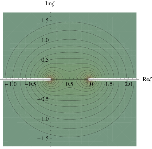
Figure 1: Plot of the hyperbolic density $\rho$ on the twice-punctured plane $Y(2)$. The function $\rho(\zeta,\bar{\zeta})$ grows to infinity at each of the punctures $\zeta=0,1$ and tends to zero for $\zeta\rightarrow\infty$. The white slots are due to the branch cuts of $\mathcal{K}$, being an artifact produced by the limited numerical precision of the graphics software used.

In principle, the cosmological model can be studied directly on $\mathbb{C}\setminus\{0,1\}$ using the explicit metric (16). However, it is more convenient to lift to $\mathbb{H}$ or to $\mathbb{D}$ as explained in genalpha and recalled in Subsection 1.2. Among other advantages, this will allow us to illustrate the effect of projecting through the uniformization map and hence the difference between the behavior of the generalized two-field $\alpha$-attractor model defined by $Y(2)$ and that of the lifted model defined on the Poincaré half-plane.

2.5 Uniformization to the Poincaré half-plane

The group $\Gamma(2)$.

The hyperbolic surface $(Y(2),G)$ is uniformized to the Poincaré half-plane $\mathbb{H}$ with complex coordinate $\tau$ (see (1)) by the principal congruence subgroup $\Gamma(2)\subset\mathrm{PSL}(2,\mathbb{Z})$, which is defined as the kernel of the surjective group morphism $\mu_{2}:\mathrm{PSL}(2,\mathbb{Z})\rightarrow\mathrm{PSL}(2,\mathbb{Z}_{2})$ given by:

$$\mu_{2}\left(\left[\begin{array}[]{cc}a&b\\ c&d\end{array}\right]\right)\stackrel{{\scriptstyle{\rm def.}}}{{=}}\left[\begin{array}[]{cc}a\!\!\mod\!2&~{}b\!\!\mod\!2\\ c\!\!\mod\!2&~{}d\!\!\mod\!2\end{array}\right]~{}~{}.$$

In particular, $\Gamma(2)$ is a normal subgroup of $\mathrm{PSL}(2,\mathbb{Z})$. It consists of all matrices $A=\left[\begin{array}[]{cc}a&b\\ c&d\end{array}\right]\in\mathrm{PSL}(2,\mathbb{Z})$ for which $a$ and $d$ are odd and $b$ and $c$ are even. This non-Abelian group is freely generated by the two parabolic elements:

$$P_{\infty}=\left[\begin{array}[]{cc}1&2\\ 0&1\end{array}\right]~{}~{},~{}~{}P_{0}=\left[\begin{array}[]{cc}1&0\\ -2&1\end{array}\right]~{}~{},$$ (17)

which act as:

$$P_{\infty}(\tau)=\tau+2~{}~{},~{}~{}P_{0}(\tau)=\frac{\tau}{1-2\tau}~{}~{}.$$

We have $\pi_{1}(Y(2))\simeq\Gamma(2)$. Notice that $P_{0}^{-1}=\left[\begin{array}[]{cc}1&0\\ 2&1\end{array}\right]$ (which acts as $P_{0}^{-1}(\tau)=\frac{\tau}{2\tau+1}$) and that $\Gamma$ is also generated by $P_{0}^{-1}$ and $P_{\infty}$. It is known that the normalizer of $\Gamma(2)$ inside $\mathrm{PSL}(2,\mathbb{R})$ equals $\mathrm{PSL}(2,\mathbb{Z})$:

$$N(\Gamma(2))\stackrel{{\scriptstyle{\rm def.}}}{{=}}N_{\mathrm{PSL}(2,\mathbb{R})}(\Gamma(2))=\mathrm{PSL}(2,\mathbb{Z})~{}~{}.$$

We also have $N_{\mathrm{PSL}(2,\mathbb{Z})}(\Gamma(2))=\mathrm{PSL}(2,\mathbb{Z})$, since $\Gamma(2)$ is a normal subgroup of $\mathrm{PSL}(2,\mathbb{Z})$.

The anharmonic action and the anharmonic group.

The group $\mathrm{PSL}(2,\mathbb{Z}_{2})$ is isomorphic with the permutation group $S_{3}$ on three elements. This group has an isometric action on $Y(2)$ known as the anharmonic action, which permutes the three punctures of $Y(2)$ (i.e. the three cusp ends of the hyperbolic triply-punctured sphere). Moreover, $\mathrm{PSL}(2,\mathbb{Z}_{2})$ can be identified with the quotient $\mathrm{PSL}(2,\mathbb{Z})/\Gamma(2)$ and there exists a canonical lift of $\mathrm{PSL}(2,\mathbb{Z}_{2})$ to a subgroup $\mathfrak{B}$ of $\mathrm{PSL}(2,\mathbb{Z})$ known as the anharmonic group. Viewing the anharmonic group as a subgroup of the Möbius group $\mathrm{PSL}(2,\mathbb{C})$, this allows one to describe the anharmonic action of $\mathrm{PSL}(2,\mathbb{Z}_{2})\simeq S_{3}$ on $Y(2)$ as the restriction to $Y(2)\subset\mathbb{C}\mathbb{P}^{1}$ of the action of six Möbius transformations of $\mathbb{C}\mathbb{P}^{1}$. We refer the reader to Appendix A for an account of this construction and for details regarding the anharmonic action on $Y(2)$.

The uniformizing map.

For $\Sigma=Y(2)$, the holomorphic covering map $\pi_{\mathbb{H}}:\mathbb{H}\rightarrow\Sigma$ is given (Ahlfors, , Chapter 7) by the elliptic modular lambda function $\lambda:\mathbb{H}\rightarrow Y(2)$, which is defined through:

$$\lambda(\tau)=\frac{\wp_{\tau}(\frac{1+\tau}{2})-\wp_{\tau}(\frac{\tau}{2})}{\wp_{\tau}(\frac{1}{2})-\wp_{\tau}(\frac{\tau}{2})}~{}~{},$$

where:

$$\wp_{\tau}(z)\stackrel{{\scriptstyle{\rm def.}}}{{=}}\frac{1}{z^{2}}+\sum_{(m,n)\in\mathbb{Z}^{2}\setminus\{(0,0)\}}\left(\frac{1}{(z-m-n\tau)^{2}}-\frac{1}{(m+n\tau)^{2}}\right)$$

is the Weierstrass elliptic function of modulus $\tau$. The function $\lambda(\tau)$ is invariant under the action of $\Gamma(2)$ on $\mathbb{H}$:

$$\lambda(\frac{a\tau+b}{c\tau+d})=\lambda(\tau)~{}~{},~{}~{}\forall A=\left[\begin{array}[]{cc}a&b\\ c&d\end{array}\right]\in\Gamma(2)$$

and satisfies:

$$\lambda(\tau+1)=\frac{\lambda(\tau)}{\lambda(\tau)-1}~{}~{},~{}~{}\lambda(-\frac{1}{\tau})=1-\lambda(\tau)~{}~{}.$$

The fundamental polygons for uniformization of $Y(2)$ to the Poincaré half-plane and to the Poincaré disk can be found in Appendix B, to which we refer the interested reader for details. The same appendix explains the construction of canonical coordinates near each cusp end of $Y(2)$ (see genalpha ).

2.6 A multivalued inverse of $\lambda$

A multivalued inverse $\mu$ of the holomorphic covering map $\lambda$ is given as follows in terms of hypergeometric functions:

$$\tau=\mu(\zeta)=\mathbf{i}\frac{~{}_{2}F_{1}(\frac{1}{2},\frac{1}{2};1|1-\zeta)}{~{}_{2}F_{1}(\frac{1}{2},\frac{1}{2};1|\zeta)}~{}~{}.$$ (18)

This multivalued analytic function has monodromy around the punctures $\zeta=0,1,\infty$, generated respectively by the transformations $P_{0}$, $P_{1}\stackrel{{\scriptstyle{\rm def.}}}{{=}}P_{\infty}P_{0}$ and $P_{\infty}$. In particular, a preimage of the point $\zeta=-1$ is given by:

$$\tau_{0}=\mathbf{i}\frac{~{}_{2}F_{1}(\frac{1}{2},\frac{1}{2},1|2)}{~{}_{2}F_{1}(\frac{1}{2},\frac{1}{2};1|-1)}=1+\mathbf{i}~{}~{}.$$

This multivalued inverse of $\lambda$ is useful for identifying preimages in $\mathbb{H}$ of points on $Y(2)$ and was used in various computations presented in Section 3.

2.7 Presentation of $Y(2)$ as a branched cover of the complex plane

Let $q:\mathbb{C}\rightarrow\overline{\mathbb{C}}=\mathbb{C}\sqcup\{\infty\}\simeq\mathbb{C}\mathbb{P}^{1}$ be the rational function defined through:

$$z=q(\zeta)\stackrel{{\scriptstyle{\rm def.}}}{{=}}256\frac{(1-\zeta+\zeta^{2})^{3}}{\zeta^{2}(1-\zeta)^{2}}=256\frac{(\zeta-e^{\frac{\mathbf{i}\pi}{3}})^{3}(\zeta-e^{-\frac{\mathbf{i}\pi}{3}})^{3}}{\zeta^{2}(1-\zeta)^{2}}~{}~{},$$

which has poles at $\zeta=0$ and $\zeta=1$. This extends to a map $\bar{q}:\mathbb{C}\mathbb{P}^{1}\rightarrow\mathbb{C}\mathbb{P}^{1}$ upon setting $\bar{q}(\infty)=\infty$. The map $\bar{q}$ is invariant under the anharmonic action (A) of $\mathrm{PSL}(2,\mathbb{Z}_{2})$. Its ramification points are $z=0$, $z=2^{6}3^{3}=1728$ and $z=\infty$ and we have:

• $\bar{q}^{-1}(\{\infty\})=\{0,1,\infty\}$, each preimage point having ramification index two

• $\bar{q}^{-1}(\{0\})=\{e^{-\frac{\mathbf{i}\pi}{3}},e^{+\frac{\mathbf{i}\pi}{3}}\}$, each preimage point having ramification index three

• $\bar{q}^{-1}(\{1728\})=\{-1,\frac{1}{2},2\}$, each preimage point having ramification index two.

These special level sets of $\bar{q}$ coincide with the short orbits of the action of $\mathfrak{B}$ on $X(2)$ shown in Tables 4, 6 and 7 of Appendix A. In particular, $\bar{q}$ presents $Y(2)$ as a degree six branched cover of the complex plane with complex coordinate $z$, ramified at the points $z=0$ and $z=1728$; it is the projection map of the topological quotient $Y(2)\rightarrow Y(2)/\mathfrak{B}=\mathbb{C}$.

2.8 Quotients of $Y(2)$ by the anharmonic group $\mathfrak{B}$

Klein’s $j$-function $j:\mathbb{H}\rightarrow\mathbb{C}$ (which is invariant under the whole classical modular group $\mathrm{PSL}(2,\mathbb{Z})$) is related to the $\lambda$ function through:

$$j(\tau)=(q\circ\lambda)(\tau)=256\frac{(1-\lambda(\tau)+\lambda(\tau)^{2})^{3}}{\lambda(\tau)^{2}(1-\lambda(\tau))^{2}}~{}~{}.$$

This function presents $\mathbb{H}$ as an $\infty:1$ branched cover of the complex plane. The preimage $j^{-1}(\{z\})$ of any point $z\in\mathbb{C}$ is a full orbit of the action of $\mathrm{PSL}(2,\mathbb{Z})$ on $\mathbb{H}$. The topological quotient $\mathbb{H}/\mathrm{PSL}(2,\mathbb{Z})=Y(2)/\mathfrak{B}$ can be identified with the complex plane $\mathbb{C}$ with coordinate $z$ using the $j$-function.

One can construct a good orbifold whose underlying space is the complex plane by taking the orbifold quotient $\mathfrak{M}\stackrel{{\scriptstyle{\rm def.}}}{{=}}\mathbb{H}\mathbin{/\mkern-6.0mu/}\mathrm{PSL}(2,\mathbb{Z})=Y(2)\mathbin{/\mkern-6.0mu/}\mathfrak{B}$ instead of the topological quotient. This quotient has orbifold points located at $z=0$ and $z=1728$, with isotropy groups $\mathbb{Z}_{3}$ and $\mathbb{Z}_{2}$ respectively. It has a natural compactification given by the good orbifold $\overline{\mathfrak{M}}\stackrel{{\scriptstyle{\rm def.}}}{{=}}\mathbb{C}\mathbb{P}^{1}\mathbin{/\mkern-6.0mu/}\mathfrak{B}$, which has a further singular point at $z=\infty$ with isotropy group $\mathbb{Z}_{2}$.

Remark.

The complex plane $\mathbb{C}$ coincides with the coarse moduli space of elliptic curves. The (uncompactified) moduli stack of elliptic curves with one marked point is $\mathcal{M}=\mathbb{H}\mathbin{/\mkern-6.0mu/}\mathrm{SL}(2,\mathbb{Z})\simeq Y(2)\mathbin{/\mkern-6.0mu/}(\mathrm{C}\times\mathfrak{B})$, where $\mathrm{C}=\{-1,1\}\simeq\mathbb{Z}_{2}$ is the center of $\mathrm{SL}(2,\mathbb{Z})$. Thus $\mathfrak{M}$ is an orbifold two-fold cover of $\mathcal{M}$. On the other hand, the non-compact modular curve $Y(2)$ coincides with the coarse moduli space of elliptic curves with level two structure. The (uncompactified) moduli stack of elliptic curves with level two structure is the quotient $\mathcal{M}[2]=Y(2)\mathbin{/\mkern-6.0mu/}\mathrm{C}$, which is a six-fold cover of $\mathcal{M}$.

2.9 The orbifold hyperbolic metric induced on $\mathfrak{M}$

Since $\mathrm{PSL}(2,\mathbb{Z})$ contains elliptic elements (which have fixed points on $\mathbb{H}$), the Poincaré metric $G_{\mathbb{H}}$ does not descend through $j=q\circ\lambda$ to an ordinary Riemannian metric on the topological quotient $\mathbb{C}=\mathbb{H}/\mathrm{PSL}(2,\mathbb{Z})=Y(2)/\mathfrak{B}$ (in fact, $\mathbb{C}$ admits no complete hyperbolic metric which is compatible with its usual complex structure). Equivalently, the hyperbolic metric $G$ of $Y(2)$ does not descend to an ordinary metric on the quotient, because the action of $\mathfrak{B}$ on $Y(2)$ has orbits with non-trivial isotropy.

However, $G_{\mathbb{H}}$ (or $G$) does descend to a hyperbolic orbifold metric on $\mathfrak{M}$. This can be viewed as a metric defined on $\mathbb{C}\setminus\{0,1728\}$, with conical singularities at $z=0$ and $z=1728$. It has the form:

$$\mathrm{d}s^{2}_{0}=\rho_{0}(z,\bar{z})^{2}|\mathrm{d}z|^{2}$$

where:

$$\rho_{0}(q(\zeta),\overline{q(\zeta)})=\frac{\rho(\zeta,\bar{\zeta})}{|q^{\prime}(\zeta)|}~{}~{}\mathrm{with}~{}~{}q^{\prime}(\zeta)=\frac{(\zeta+1)(\zeta-2)(2\zeta-1)(1-\zeta+\zeta^{2})^{2}}{\zeta^{3}(\zeta-1)^{3}}~{}~{}.$$

Notice that $\rho_{0}$ tends to $0$ for $z\rightarrow\infty$ (i.e. for $\zeta=0,1$) and that it tends to $+\infty$ at the orbifold points $z=0$ and $z=1728$ (i.e. when $\zeta=e^{\pm\frac{\mathbf{i}\pi}{3}}$ and when $\zeta\in\{-1,1/2,2\}$).

2.10 Description of modular-invariant $j$-models as lifts of generalized two-field $\alpha$-attractor models

Since the orbifold metric $\rho_{0}$ has conical singularities at finite distance, it cannot be used to define an $\alpha$-attractor model in the sense of genalpha . In particular, the $\mathrm{PSL}(2,\mathbb{Z})$-invariant models (the “modular invariant $j$-models”) defined in Sch1 ; Sch2 on the Poincaré half-plane do not descend to generalized two-field $\alpha$-attractor models (in the sense of genalpha ) defined on the topological quotient $\mathbb{H}/\mathrm{PSL}(2,\mathbb{Z})=Y(2)/\mathfrak{B}=\mathbb{C}$. However, those models do descend (upon taking the quotient by $\Gamma(2)$ rather than by $\mathrm{PSL}(2,\mathbb{Z})$) to generalized two-field $\alpha$-attractor models defined on $Y(2)$, whose scalar potential $\Phi$ is invariant under the action of the anharmonic group $\mathfrak{B}$. Notice that a generalized two-field $\alpha$-attractor model defined on $Y(2)$ typically lifts through $\lambda$ to a model which is invariant only under the action of the subgroup $\Gamma(2)$ rather than under the action of the full classical modular group $\mathrm{PSL}(2,\mathbb{Z})$, since the scalar potential $\Phi$ of an $\alpha$-attractor model with scalar manifold $Y(2)$ need not be invariant under the action of $\mathfrak{B}$. As a consequence, the models of Sch1 ; Sch2 do not provide the most general lift of our $Y(2)$ models to the Poincaré half-plane. To describe the most general lift, one must require invariance of the half-plane model only under $\Gamma(2)$ rather than under $\mathrm{PSL}(2,\mathbb{Z})$.

3 Cosmological trajectories

In this section, we present numerical examples of cosmological trajectories in generalized two-field $\alpha$-attractor models defined by $Y(2)$ and in the corresponding lifted models, for certain simple but natural choices of globally well-behaved scalar potentials, with $\alpha=\frac{M_{0}}{3}$.

3.1 Globally well-behaved scalar potentials on $Y(2)$

Let $\rho=|\zeta|$ and $\theta=\arg(\zeta)$. The embedding (15) into the end compactification shows that a smooth potential $\Phi:Y(2)=\mathbb{C}\setminus\{0,1\}\rightarrow\mathbb{R}$ is globally well-behaved iff there exists a smooth map $\hat{\Phi}:X(2)=\mathbb{C}\mathbb{P}^{1}\simeq\mathrm{S}^{2}\rightarrow\mathbb{R}$ such that:

$$\Phi(\rho,\theta)=\hat{\Phi}(2\operatorname{arccot}(\rho),\theta)~{}~{}.$$

Expanding $\hat{\Phi}$ into real (a.k.a. tesseral) spherical harmonics $Y_{lm}$:

$$\hat{\Phi}(\psi,\theta)=\sum_{l=0}^{\infty}\sum_{m=-l}^{l}D_{lm}Y_{lm}(\psi,\theta)$$

(where $D_{lm}$ are real constants) gives the uniformly-convergent expansion:

$$\Phi(\rho,\theta)=\sum_{l=0}^{\infty}\sum_{m=-l}^{l}D_{lm}Y_{lm}(2\operatorname{arccot}(\rho),\theta)~{}~{}.$$

Some simple choices for $\hat{\Phi}$ are as follows:

• The following linear combinations of the $s$ ($Y_{00}$) and $p_{z}$ ($Y_{10}$) orbitals:

  $$\hat{\Phi}_{+}(\psi)=M_{0}\cos^{2}\left(\frac{\psi}{2}\right)~{}~{},~{}~{}\hat{\Phi}_{-}(\psi)=M_{0}\sin^{2}\left(\frac{\psi}{2}\right)~{}~{},$$ (19)

• The following linear combination of the $s$ ($Y_{00}$) and $p_{x}$ ($Y_{11}$) orbitals:

  $$\hat{\Phi}_{0}(\psi,\theta)=M_{0}(1+\sin\psi\cos\theta)=M_{0}(1+x_{1})~{}~{}.$$ (20)

• The following linear combination of the $s$ ($Y_{00}$), $d_{z^{2}}$ ($Y_{20}$) and $d_{x^{2}-y^{2}}$ ($Y_{22}$) orbitals:

  $$\hat{\Phi}_{1}(\psi,\theta)=M_{0}[1-\sin^{2}(\psi)\cos^{2}(\theta)+\cos^{2}(\psi)]=M_{0}\left[1-x_{1}^{2}+x_{3}^{2}\right]~{}~{}.$$

These choices give:

$$\Phi_{+}=M_{0}\frac{\rho^{2}}{1+\rho^{2}}~{}~{},~{}~{}\Phi_{-}=M_{0}\frac{1}{1+\rho^{2}}~{}~{},~{}~{}\Phi_{0}=M_{0}\left[1+\frac{2\rho\cos\theta}{1+\rho^{2}}\right]~{}~{},$$

$$\Phi_{1}=M_{0}\left[1-\frac{4\rho^{2}}{(1+\rho^{2})^{2}}\cos^{2}\theta+\frac{(1-\rho^{2})^{2}}{(1+\rho^{2})^{2}}\right]~{}~{}.$$ (21)

Notice that all of these potentials are compactly Morse in the sense of genalpha . The extrema of the extended potentials are shown in Table 1.

extremum in coords. $(\psi,\theta)$	$\psi=0$	$\psi=\pi$	$(\psi,\theta)=(\frac{\pi}{2},0)$	$(\psi,\theta)=(\frac{\pi}{2},\pi)$
extremum in coord. $\zeta$	$\zeta=\infty$	$\zeta=0$	$\zeta=1$	$\zeta=-1$
$\hat{\Phi}_{+}/M_{0}$	max (1)	min (0)	none (1/2)	none (1/2)
$\hat{\Phi}_{-}/M_{0}$	min (0)	max (1)	none (1/2)	none (1/2)
$\hat{\Phi}_{0}/M_{0}$	none (1)	none (1)	max (2)	min (0)
$\hat{\Phi}_{1}/M_{0}$	max (2)	max (2)	min (0)	min (0)

Table 1: Extrema of extended potentials. In parantheses, we indicate the value of $\hat{\Phi}/M_{0}$ at the extremum point. Notice that only $\Phi_{0}$ and $\Phi_{1}$ have extrema inside $Y(2)$. Also notice that each of the cusp points is an extremum point of $\hat{\Phi}_{1}$.

Since $\tau_{0}=1+\mathbf{i}\in\mathbb{H}$ is an inverse image of the point $\zeta=-1$, the lifted potentials ${\tilde{\Phi}}_{0}$ and ${\tilde{\Phi}}_{1}$ have local minima (equal to zero) at the point $\tau_{0}$ and at each of its images through the action of $\Gamma(2)$. These local minima accumulate toward any point on the conformal boundary $\partial_{\infty}\mathbb{H}$. The level sets of the potentials $\Phi_{\pm}$, $\Phi_{0}$ and $\Phi_{1}$ and of their lifts to $\mathbb{H}$ are shown in Figures 3, 6, 11 and 15 of the next subsection. Notice that none of these potentials is invariant under the anharmonic group $\mathfrak{B}$.

3.2 Some examples of cosmological trajectories

In this subsection, we present four numerically computed trajectories (drawn in black, red, magenta and yellow) for each of the potentials $\Phi_{\pm},\Phi_{0}$ and $\Phi_{1}$. These trajectories were chosen such that their lifts to $\mathbb{H}$ have the initial conditions at cosmological time $t=0$ shown in Table 2, irrespective of the choice of the scalar potential.

trajectory	$\tau_{0}$	$\tilde{v}_{0}$
black	$0.4+0.5\mathbf{i}$	$0.3+\mathbf{i}$
red	$1.4+0.5\mathbf{i}$	$0.1+0.2\mathbf{i}$
magenta	$0.2+0.7\mathbf{i}$	$0.7+0.5\mathbf{i}$
yellow	$0.3+0.5\mathbf{i}$	$0$

Table 2: Initial conditions for four trajectories on the Poincaré half-plane.

For each of the four scalar potentials, Table 3 shows which of these initial conditions belong to the inflation region of the corresponding lifted potential. Trajectories which satisfy this condition produce a cosmological scale factor $a(t)$ which is a convex and increasing function of $t$ for some interval starting at $t=0$. Notice that this condition cannot be satisfied when $\Phi=0$.

trajectory	$\Phi_{+}$	$\Phi_{-}$	$\Phi_{0}$	$\Phi_{1}$
black	no	no	no	no
red	yes	no	yes	yes
magenta	no	no	yes	no
yellow	yes	yes	yes	yes

Table 3: Inflationary character of the initial conditions of Table 2 with respect to the scalar potentials $\Phi_{\pm}$, $\Phi_{0}$ and $\Phi_{1}$. The table indicates “yes” when $(\tau_{0},\tilde{v}_{0})$ belongs to the inflation region of ${\tilde{\Phi}}$ and “no” otherwise.

Trajectories for $\Phi=0$.

To understand the effect of the hyperbolic geometry, it is instructive to consider first the case when the scalar potential vanishes identically. In this situation, the yellow trajectory (which has vanishing initial speed) remains stationary for all values of the cosmological time, as can be seen by inspecting the system (5) and using the Picard-Lindelöf theorem. Any other trajectory on $Y(2)$ ultimately evolves toward one of the cusp points, while its lift to the Poincaré half-plane evolves toward the conformal boundary $\partial_{\infty}\mathbb{H}$. Hence each cusp point exerts an attractive “effective force”. As shown in Figure 2, each projected trajectory spirals in a complicated manner around the cusp points of $Y(2)$, until eventually “falling” deep inside one of the cusp neighborhoods, where it evolves when $t\rightarrow+\infty$ toward the corresponding ideal point. In the figures, the initial point of each trajectory is shown as a thick dot.

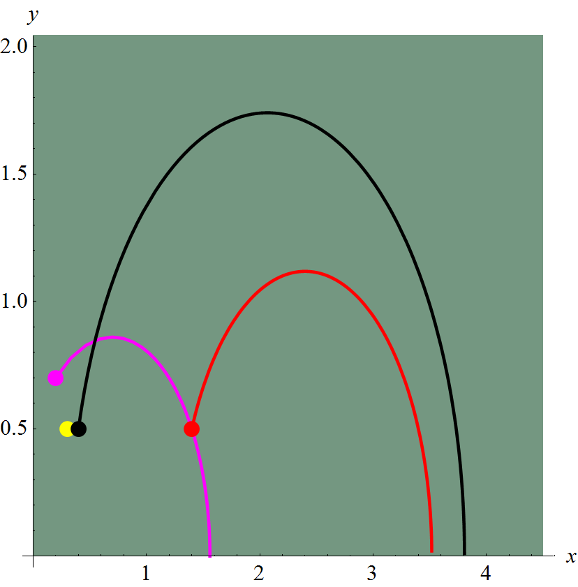
(a) Trajectories for ${\tilde{\Phi}}=0$ on the Poincaré half-plane. The solution shown in yellow is stationary.

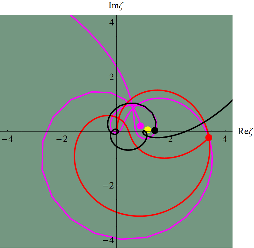
(b) Projection to $Y(2)$ of the trajectories shown at the left.

Figure 2: Numerical solutions for $\Phi=0$ and $\alpha=\frac{M_{0}}{3}$.

Trajectories for $\Phi_{+}$.

The level sets of the potential $\Phi_{+}$ and of its lift ${\tilde{\Phi}}_{+}$ to the Poincaré half-plane are shown in Figure 3. This potential has a vanishing infimum at the cusp $\zeta=0$ and tends to its supremum (which equals $M_{0}$) for $\xi\rightarrow\infty$.

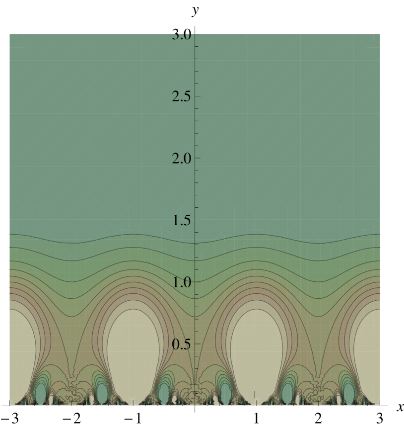
(a) Level plot of ${\tilde{\Phi}}_{+}/M_{0}$ on the Poincaré half-plane.

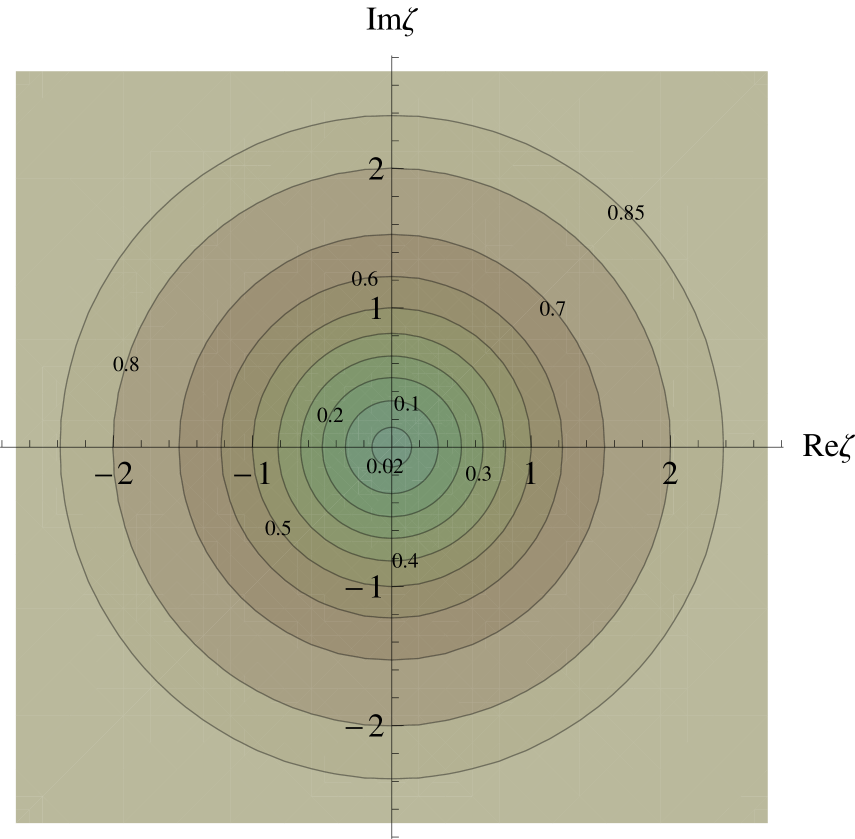
(b) Level plot of $\Phi_{+}/M_{0}$ on the twice punctured plane.

Figure 3: Level plots of ${\tilde{\Phi}}_{+}/M_{0}$ and $\Phi_{+}/M_{0}$. Darker tones indicate lower values.

The four trajectories whose lifts have the initial conditions given in Table 2 are shown in Figure 4. Due to the effect of the potential, the projected yellow trajectory (which starts with initial velocity zero) evolves toward the cusp point at $\zeta=0$, as do the other three trajectories. For clarity, Figure 4 shows only a small portion of the trajectories on the Poincaré half-plane.

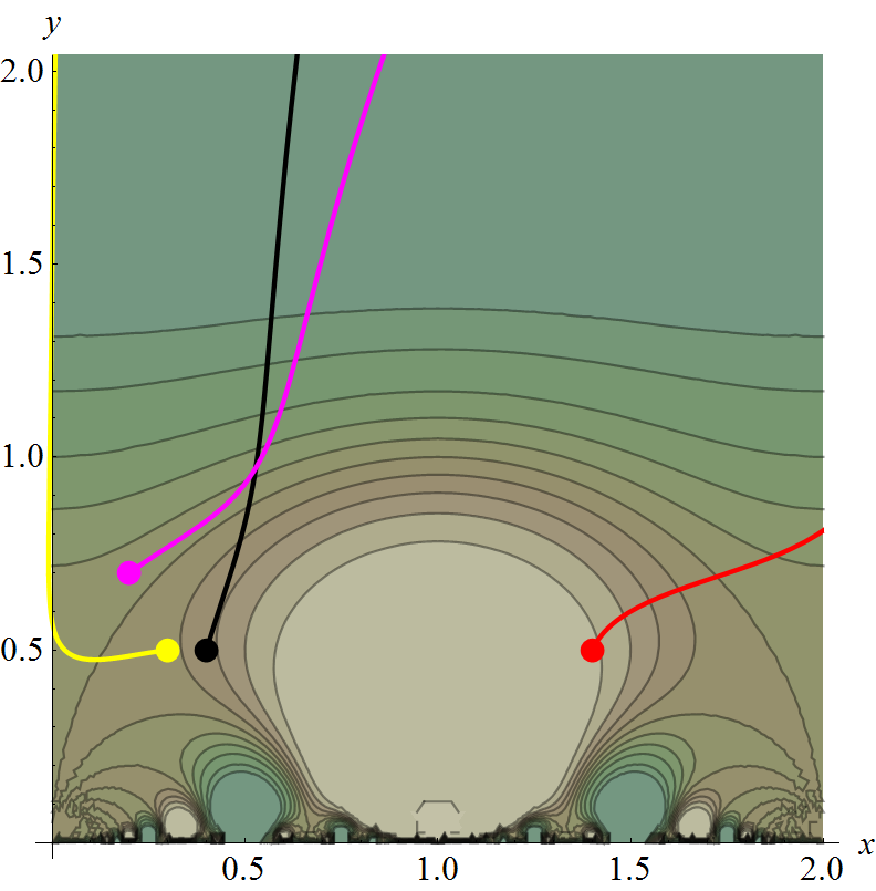
(a) Trajectories for ${\tilde{\Phi}}={\tilde{\Phi}}_{+}$ on the Poincaré half-plane.

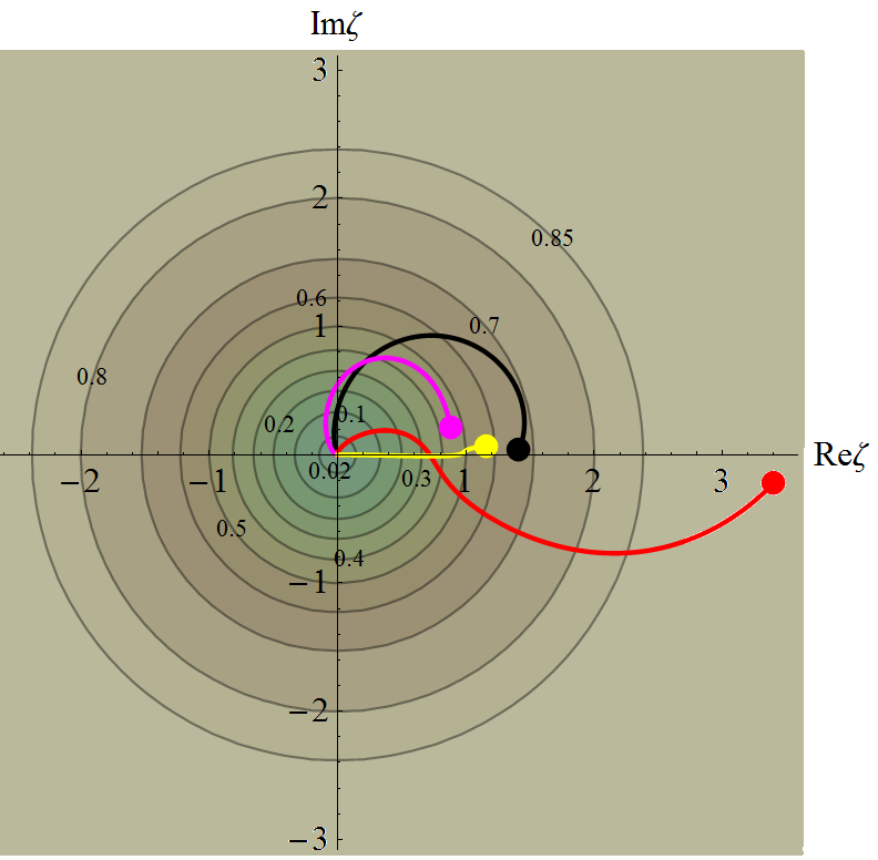
(b) Projection to $Y(2)$ of the trajectories shown at the left.

Figure 4: Numerical solutions for $\Phi=\Phi_{+}$ and $\alpha=\frac{M_{0}}{3}$.

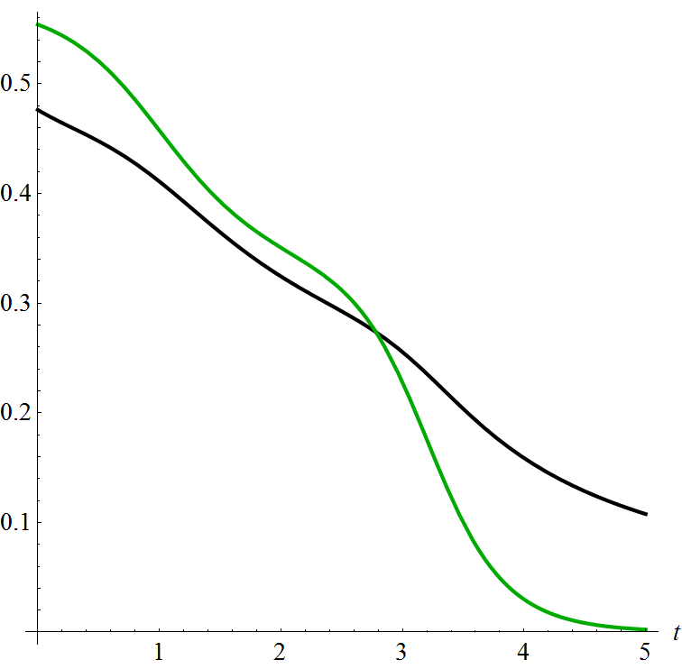
(a) Plot of $H(t)/\sqrt{M_{0}}$ and $H_{c}(t)/\sqrt{M_{0}}$ for the red trajectory.

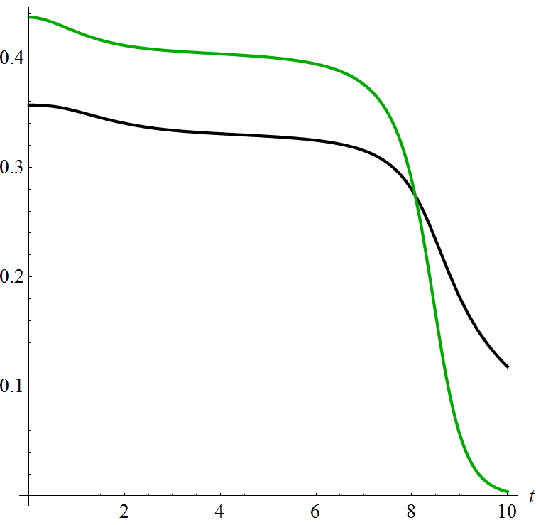
(b) Plot of $H(t)/\sqrt{M_{0}}$ and $H_{c}(t)/\sqrt{M_{0}}$ for the yellow trajectory.

Figure 5: Plot of $H(t)/\sqrt{M_{0}}$ (black) and $H_{c}(t)/\sqrt{M_{0}}$ (green) for the red and yellow trajectories with $\Phi=\Phi_{+}$ and $\alpha=\frac{M_{0}}{3}$.

Figure 5 shows the evolution of the Hubble parameter $H(t)$ for the red and yellow trajectories, comparing it with the critical Hubble parameter $H_{c}(t)\stackrel{{\scriptstyle{\rm def.}}}{{=}}H_{c}(\varphi(t))$ along that trajectory. For the clarity of the figure we represent here the evolution of $H(t)$ and $H_{c}(t)$ only up to $t<5s$. As clear from the figure, the tangent vectors of these trajectories lie within the inflation region of $\Phi_{+}$ for some time interval starting at $t=0$, thus displaying the behavior expected in inflation.

Trajectories for $\Phi_{-}$.

The level sets of the potential $\Phi_{-}$ and of its lift ${\tilde{\Phi}}_{-}$ to the Poincaré half-plane are shown in Figure 6. This potential has a supremum (which equals $M_{0}$) at the puncture $\zeta=0$ and tends to its vanishing infimum for $\zeta\rightarrow+\infty$.

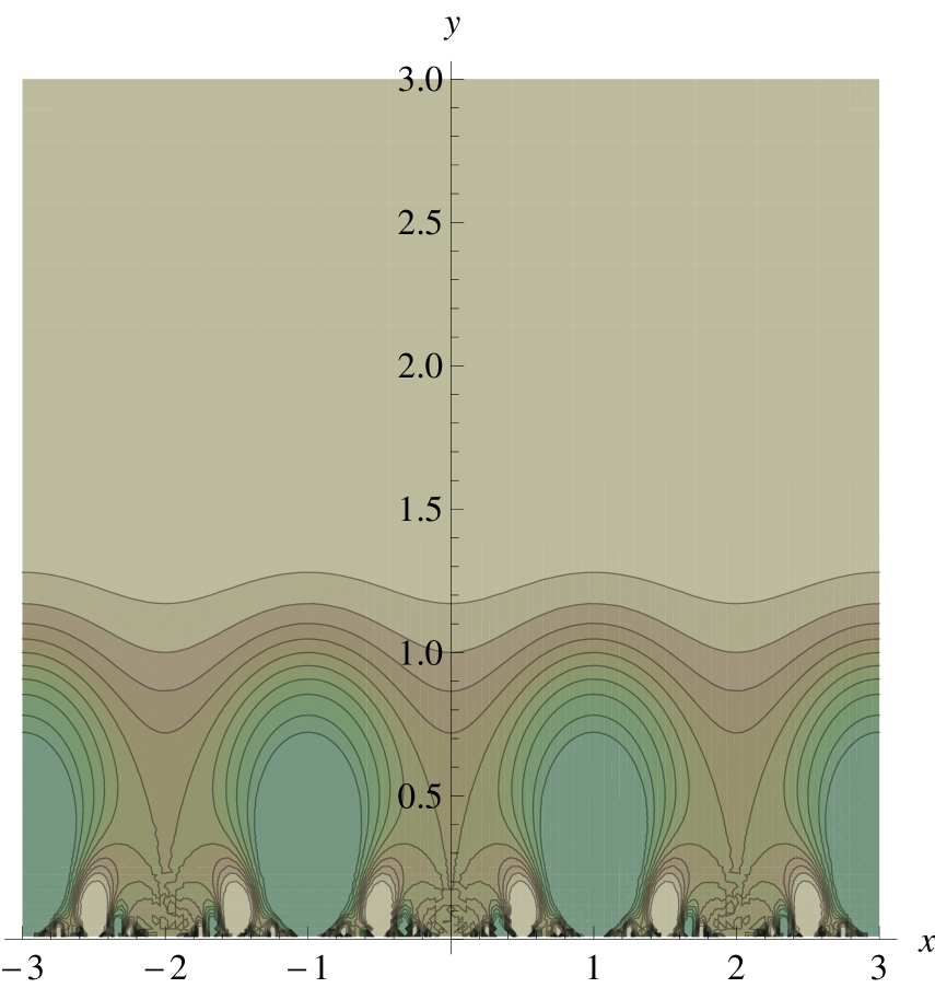
(a) Level plot of ${\tilde{\Phi}}_{-}/M_{0}$ on the Poincaré half-plane.

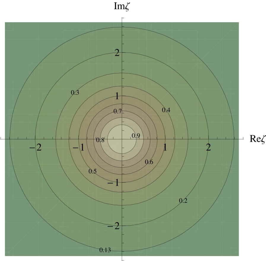
(b) Level plot of $\Phi_{-}/M_{-}$ on the twice punctured plane.

Figure 6: Level plots of ${\tilde{\Phi}}_{-}/M_{0}$ and $\Phi_{-}/M_{0}$. Darker tones indicate lower values.

Figure 7 shows the lifted trajectories with initial conditions given in Table 2 and their projections through the uniformization map. Despite the repulsive force produced by the potential (which is counterbalanced by the attractive effective force produced by the hyperbolic geometry of the cusp), the yellow trajectory evolves toward the cusp point $\zeta=0$. As shown in Figure 8, the projected magenta trajectory evolves toward the cusp at infinity, while the projected red and black trajectories (which, for clarity, are not fully shown in Figure 7) evolve slowly toward a point located beyond the cusp, at $\zeta=2$, where they appear to stop after winding around it a few times in a complicated manner. For more details of these two trajectories see Figure 8 and Figure 9. In this example, the repulsive force exerted by the potential is weaker that the effective attraction produced by the cusp at the origin due to the hyperbolic metric.

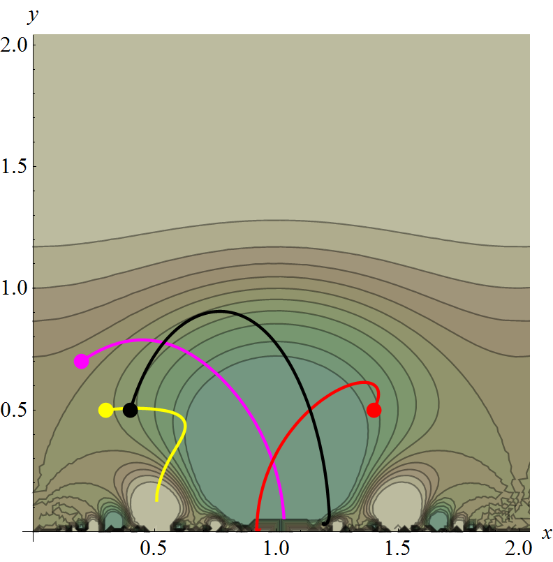
(a) Trajectories for ${\tilde{\Phi}}={\tilde{\Phi}}_{-}$ on the Poincaré half-plane.

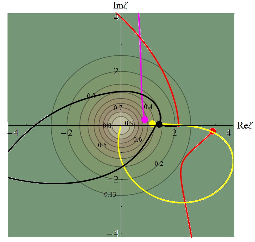
(b) Projection to $Y(2)$ of the trajectories shown at the left. For clarity, we show only the region around the puncture $\zeta=0$.

Figure 7: Numerical solutions for $\Phi=\Phi_{-}$ and $\alpha=\frac{M_{0}}{3}$.

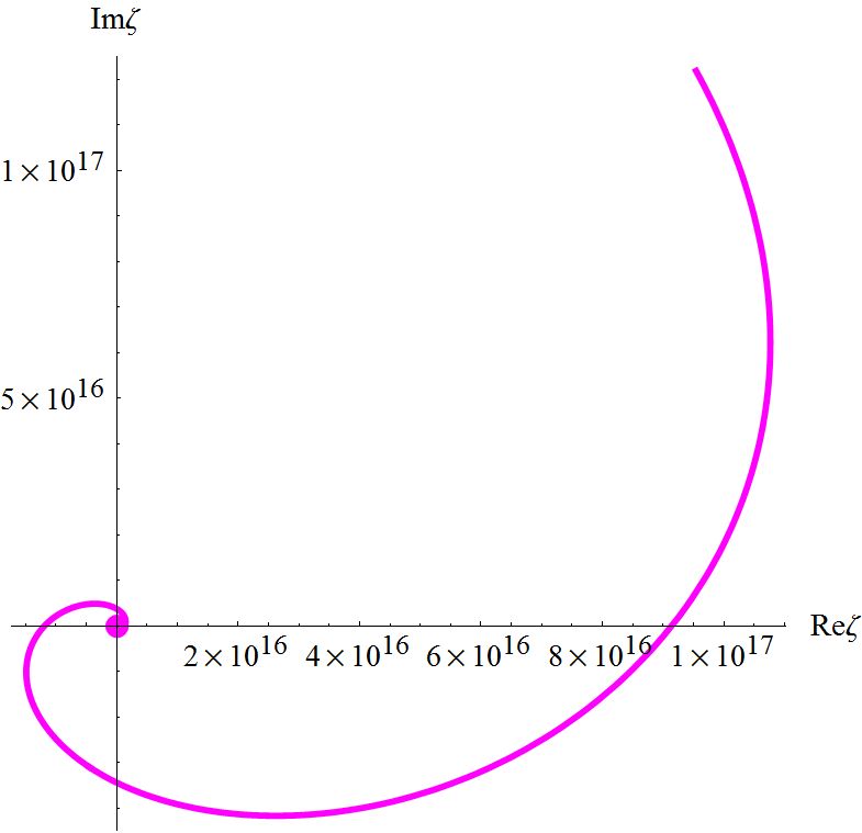
(a) Projected magenta trajectory for the potential $\Phi_{-}$.

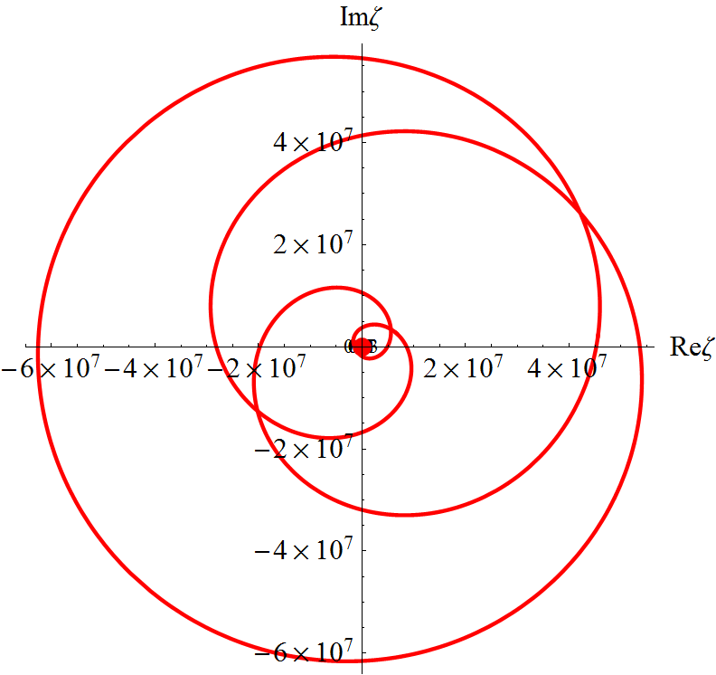
(b) Projected red trajectory for the potential $\Phi_{-}$.

Figure 8: Large scale view of the red and magenta trajectories for the potential $\Phi_{-}$ with $\alpha=\frac{M_{0}}{3}$.

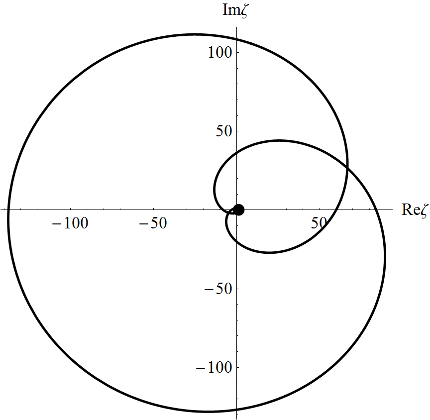
(a) Large scale view of the projected black trajectory for the potential $\Phi_{-}$

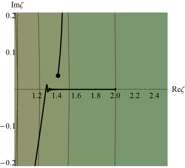
(b) Detail of the beginning and end of the projected black trajectory for the potential $\Phi_{-}$

Figure 9: The projected black trajectory for the potential $\Phi_{-}$ with $\alpha=\frac{M_{0}}{3}$.

Figure 10 shows the evolution of the Hubble parameter $H(t)$ along the yellow and black trajectories.

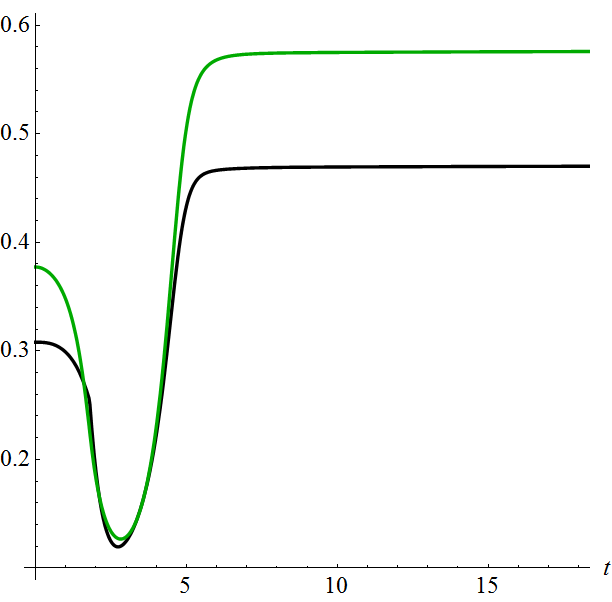
(a) Plot of $H(t)/\sqrt{M_{0}}$ and $H_{c}(t)/\sqrt{M_{0}}$ for the yellow trajectory. This trajectory produces inflation for small $t$, then exits the inflation regime and re-enters it at some later time.

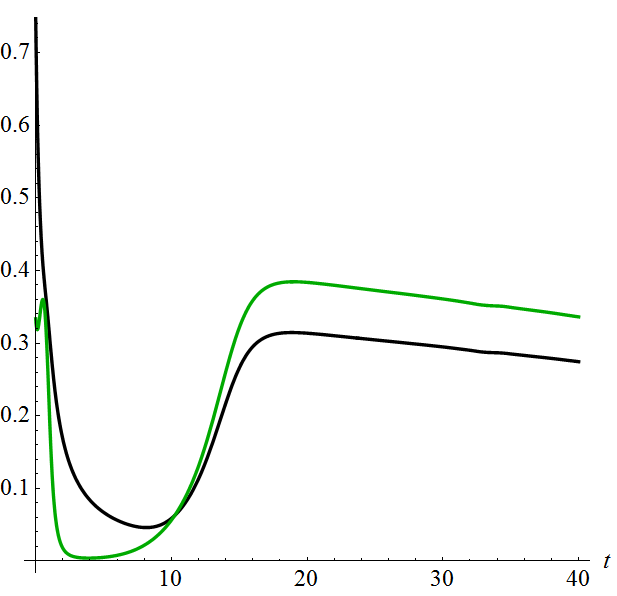
(b) Plot of $H(t)/\sqrt{M_{0}}$ and $H_{c}(t)/\sqrt{M_{0}}$ for the black trajectory. This trajectory does not produce inflation for small $t$, but it enters the inflation regime at later times.

Figure 10: Plot of $H(t)/\sqrt{M_{0}}$ (black) and $H_{c}(t)/\sqrt{M_{0}}$ (green) for the yellow and black trajectories with $\Phi=\Phi_{-}$ and $\alpha=\frac{M_{0}}{3}$.

Trajectories for $\Phi_{0}$.

The level sets of the potential $\Phi_{0}$ and of its lift ${\tilde{\Phi}}_{0}$ to the Poincaré half-plane are shown in Figure 11. This potential has a supremum (which equals $2M_{0}$) at the cusp $\zeta=1$ and a vanishing minimum at the point $\zeta=-1$, which lies inside $Y(2)$.

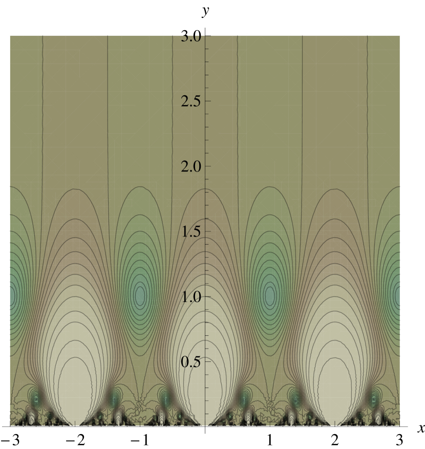
(a) Level plot of ${\tilde{\Phi}}_{0}/M_{0}$ on the Poincaré half-plane.

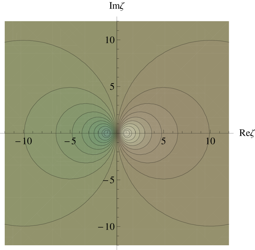
(b) Level plot of $\Phi_{0}/M_{0}$ on the twice punctured plane.

Figure 11: Level plots of ${\tilde{\Phi}}_{0}/M_{0}$ and $\Phi_{0}/M_{0}$. Darker tones indicate lower values.

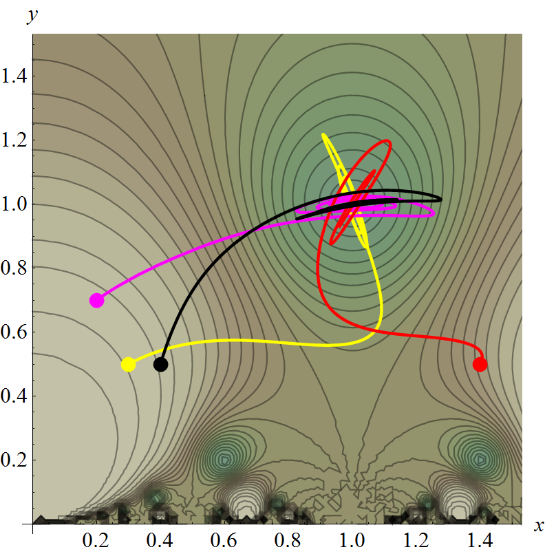
(a) Trajectories for ${\tilde{\Phi}}={\tilde{\Phi}}_{0}$ on the Poincaré half-plane.

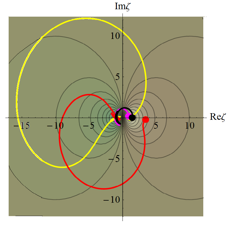
(b) Projection to $Y(2)$ of the trajectories shown at the left.

Figure 12: Numerical solutions for $\Phi=\Phi_{0}$ and $\alpha=\frac{M_{0}}{3}$.

Figure 12 shows the four lifted and projected trajectories with initial conditions given in Table 2. All four trajectories eventually evolve toward the minimum point $\zeta=-1$ of $\Phi_{0}$, after spiraling around it in a complicated manner (see the detail of these trajectories shown in Figure 13). Figure 14 shows the time evolution of the Hubble parameter along the red and magenta trajectories, both of which lead to inflation for some time interval starting at $t=0$.

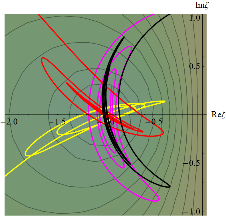
Figure 13: Detail of the projected trajectories close to the minimum of $\Phi_{0}$, for $\alpha=\frac{M_{0}}{3}$.

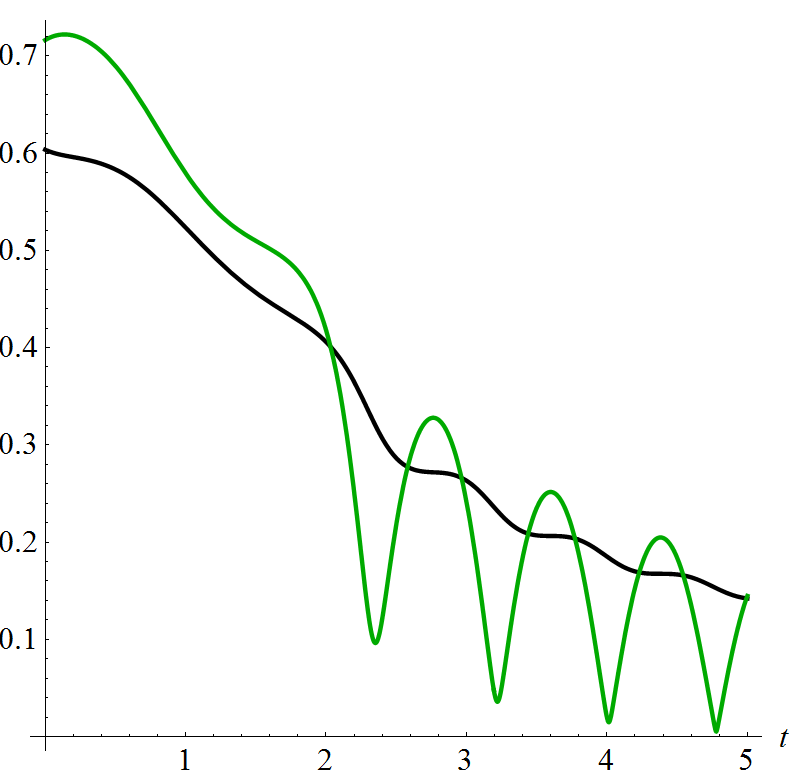
(a) Plot of $H(t)/\sqrt{M_{0}}$ and $H_{c}(t)/\sqrt{M_{0}}$ for the red trajectory.

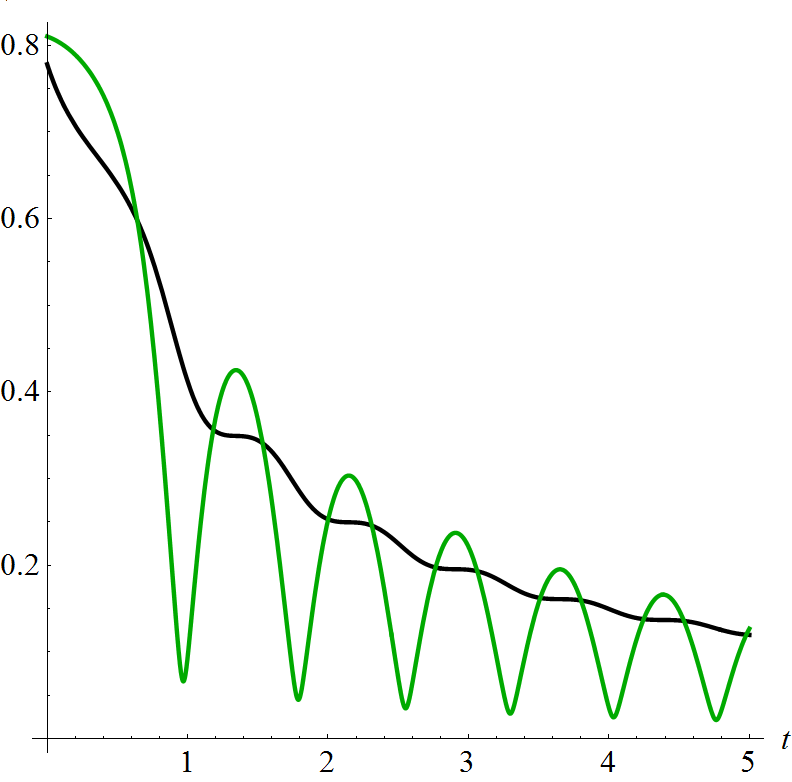
(b) Plot of $H(t)/\sqrt{M_{0}}$ and $H_{c}(t)/\sqrt{M_{0}}$ for the magenta trajectory.

Figure 14: Plot of $H(t)/\sqrt{M_{0}}$ (black) and $H_{c}(t)/\sqrt{M_{0}}$ (green) for the red and magenta trajectories with $\Phi=\Phi_{0}$ and $\alpha=\frac{M_{0}}{3}$.

Trajectories for $\Phi_{1}$.

The level sets of the potential $\Phi_{1}$ and of its lift ${\tilde{\Phi}}_{1}$ to the Poincaré half-plane are shown in Figure 15.

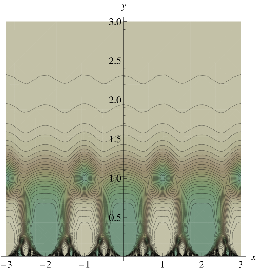
(a) Level plot of ${\tilde{\Phi}}_{1}/M_{0}$ on the Poincaré half-plane.

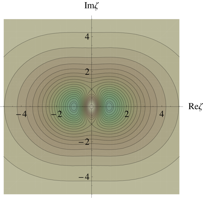
(b) Level plot of $\Phi_{1}/M_{0}$ on the twice punctured plane.

Figure 15: Level plots of ${\tilde{\Phi}}_{1}/M_{0}$ and $\Phi_{1}/M_{0}$. Darker tones indicate lower values.

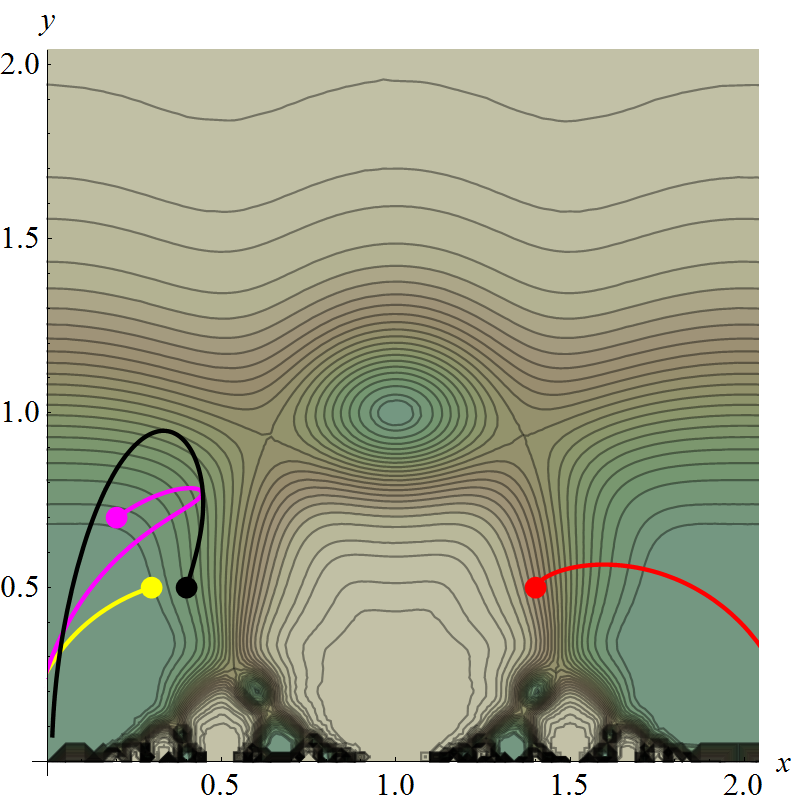
(a) Trajectories for ${\tilde{\Phi}}={\tilde{\Phi}}_{1}$ on the Poincaré half-plane.

​​​​

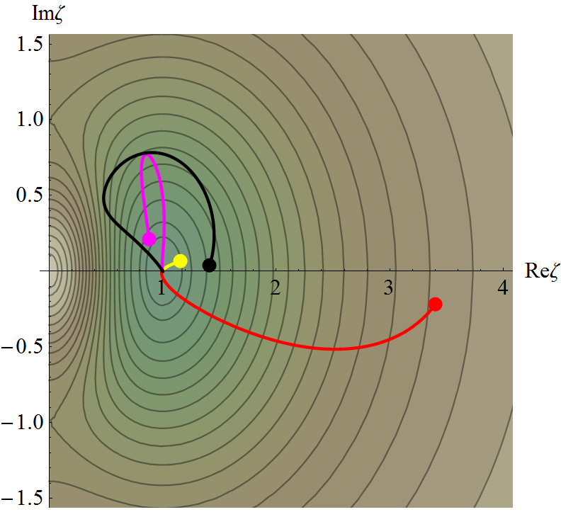
(b) Projection to $Y(2)$ of the trajectories shown at the left.

Figure 16: Numerical solutions for $\Phi=\Phi_{1}$ and $\alpha=\frac{M_{0}}{3}$.

At the cusp points, this potential tends either to its vanishing infimum (for $\zeta=1$) or to its supremum, which equals $2M_{0}$ (for $\zeta=0,\infty$). Furthermore, it has a minimum (equal to zero) at the point $\zeta=-1$, which lies inside $Y(2)$.

The four lifted trajectories with initial conditions given in Table 2 and their projections to $Y(2)$ are shown in Figure 16. All four projected trajectories evolve toward the cusp point $\zeta=1$, due to the combined effect of the potential (which has an infimum there) and of the effective attractive force produced by the cusp.

Figure 17 shows the time evolution of the Hubble parameter for the red and yellow trajectories, both of which lead to inflation for some (relatively short) cosmological time interval starting at $t=0$.

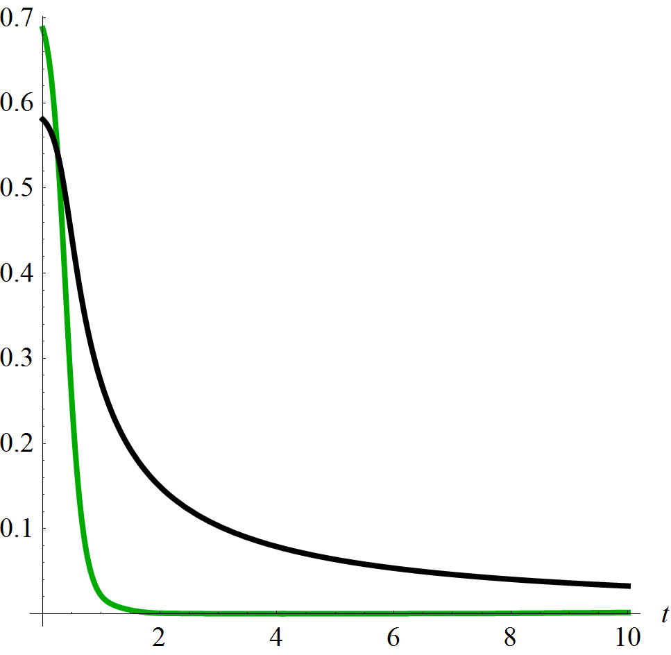
(a) Plot of $H(t)/\sqrt{M_{0}}$ and $H_{c}(t)/\sqrt{M_{0}}$ for the red trajectory.

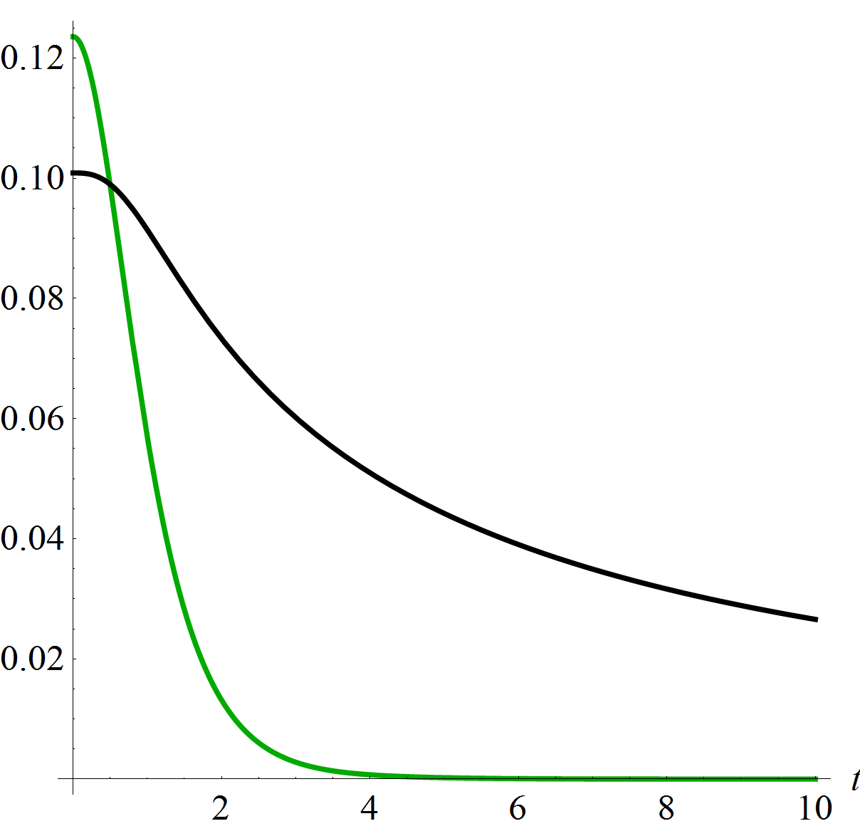
(b) Plot of $H(t)/\sqrt{M_{0}}$ and $H_{c}(t)/\sqrt{M_{0}}$ for the yellow trajectory.

Figure 17: Plot of $H(t)/\sqrt{M_{0}}$ (black) and $H_{c}(t)/\sqrt{M_{0}}$ (green) for the red and yellow trajectories with $\Phi=\Phi_{1}$ at $\alpha=\frac{M_{0}}{3}$.

The number of efolds ${\cal N}$ is given by integrating $H(t)$ over the first inflationary time interval:

$${\cal N}=\int_{0}^{t_{I}}H(t)\mathrm{d}t$$ (22)

For all the four trajectories with initial conditions given in Table 2, calculating the number of efolds for those which start in inflationary regime (see Table 3) we find values between 0.05 and 3.55, which are smaller than the values of between 50-60 efolds expected by phenomenological measurements. Nevertheless, we will show in the next subsection that we can also find trajectories with 50-60 efolds.

3.3 Examples of cosmological trajectories with 50–60 efolds

Trajectory for $\Phi_{+}$.

Choosing the initial conditions $\tau_{0}=0.99+0.41\mathbf{i}$  and ${\tilde{v}}_{0}=0$, the trajectory obtained will have ${\cal N}=58.8$ number of efolds. (See Figs. 18 and 19.) With a small variation of $y_{0}$ we can vary the number of efolds between 50 and 60, for example when $\tau_{0}=0.99+0.415\mathbf{i}$ we get ${\cal N}=50.3$ efolds.

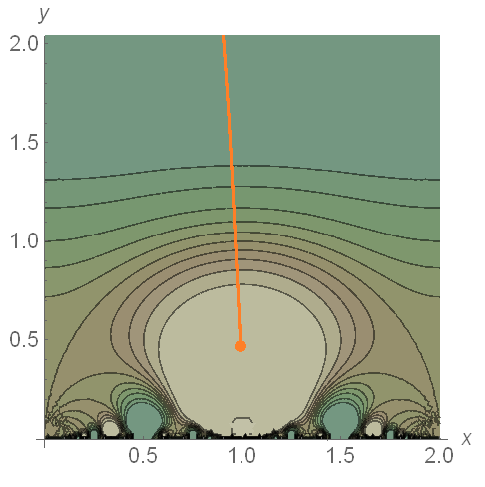
(a) Trajectory for ${\tilde{\Phi}}_{+}/M_{0}$ on the Poincaré half-plane.

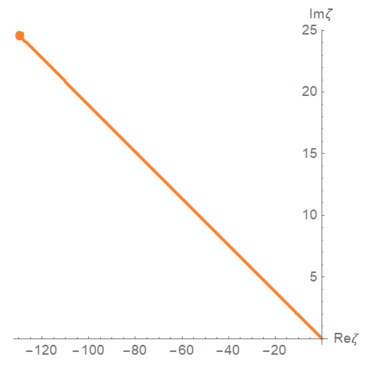
(b) Projection to $Y(2)$ of the trajectory shown at the left.

Figure 18: Numerical solution for the orange trajectory with initial conditions $\tau_{0}=0.99+0.41\mathbf{i}$ and ${\tilde{v}}_{0}=0$ in the potential $\Phi=\Phi_{+}$ when $\alpha=\frac{M_{0}}{3}$.

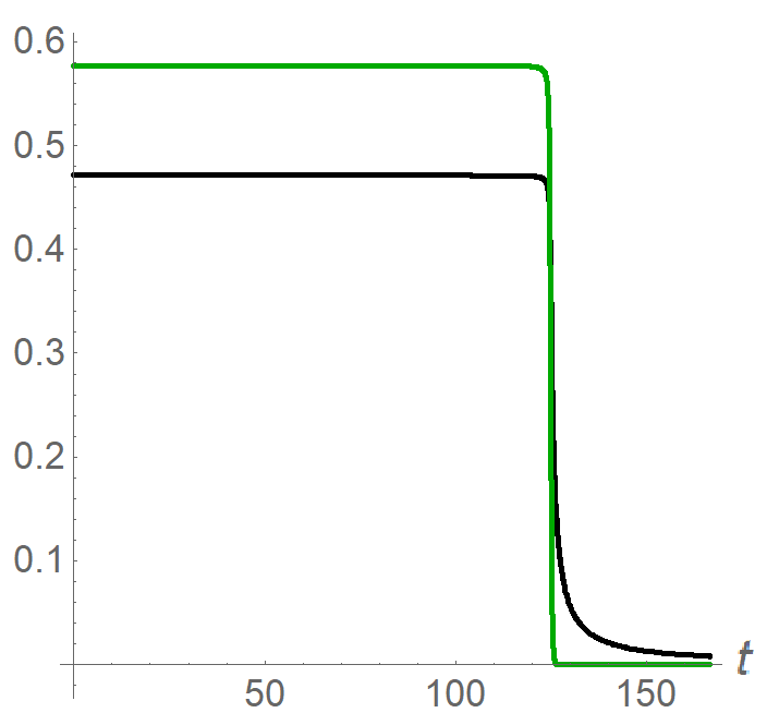
Figure 19: Plot of $H(t)/\sqrt{M_{0}}$ (black) and $H_{c}(t)/\sqrt{M_{0}}$ (green) for the orange trajectory in the potential $\Phi=\Phi_{+}$ when $\alpha=\frac{M_{0}}{3}$.

Trajectory for $\Phi_{-}$.

Choosing the initial conditions $\tau_{0}=0.198+0.3\mathbf{i}$  and ${\tilde{v}}_{0}=0$, the trajectory obtained will have ${\cal N}=56$ efolds. (See Figs. 20 and 21.)

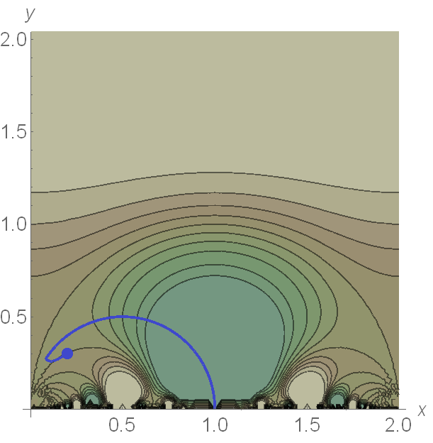
(a) Trajectory for ${\tilde{\Phi}}_{-}/M_{0}$ on the Poincaré half-plane.

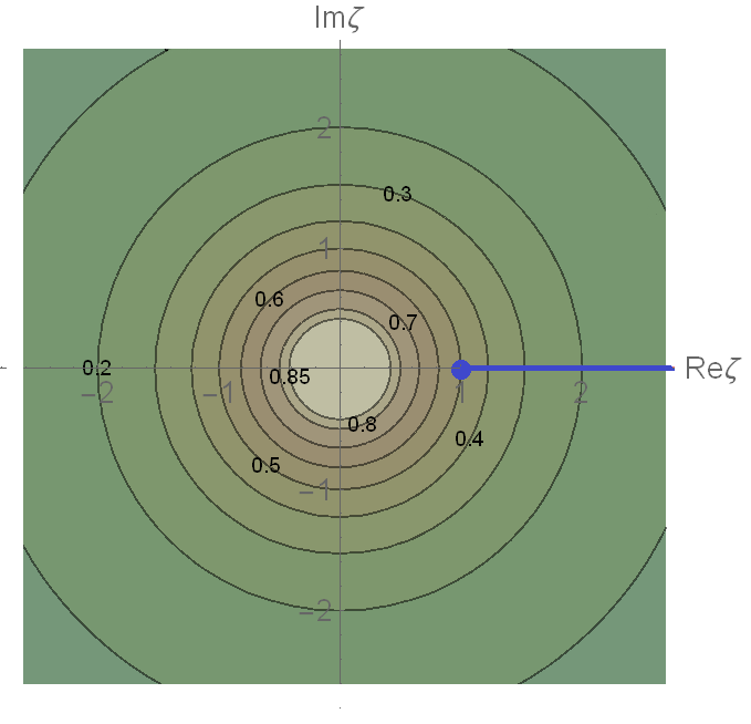
(b) Projection to $Y(2)$ of the trajectory shown at the left.

Figure 20: Numerical solution for the blue trajectory with initial conditions $\tau_{0}=0.198+0.3\mathbf{i}$ and ${\tilde{v}}_{0}=0$ in the potential $\Phi=\Phi_{-}$ when $\alpha=\frac{M_{0}}{3}$.

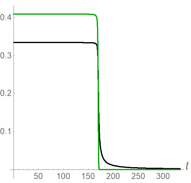
Figure 21: Plot of $H(t)/\sqrt{M_{0}}$ (black) and $H_{c}(t)/\sqrt{M_{0}}$ (green) for the blue trajectory in the potential $\Phi=\Phi_{-}$ when $\alpha=\frac{M_{0}}{3}$.

4 The gradient flow approximation

In this section, we explain how the gradient flow approximation of genalpha can be used to extract information about inflationary trajectories and the number of efolds. In particular, we apply this approximation in the vicinity of cusp ends, discussing a class of scalar potentials for which certain special inflationary trajectories produce any number of efolds within this approximation, including the observationally favored number of $50-60$ efolds. Finally, we construct explicit gradient flow trajectories of this type for those well-behaved scalar potentials which have an asymptotic rotational symmetry around cusp ends.

4.1 The gradient flow approximation in general two-field models

We first recall the gradient flow approximation of genalpha for a general two-field cosmological model (with flat FLRW spatial section) having scalar manifold $(\Sigma,{\mathcal{G}})$. As explained in loc. cit., this is the least restrictive of a ladder of increasingly constraining approximations (of which the most restrictive is the well-known SRST approximation). As shown in genalpha , the SRST approximation is of limited usefulness in the study of generalized two-field $\alpha$-attractor models, since it can fail near cusp ends. Since we are especially interested in the vicinity of such ends, we cannot rely on SRST methods, so we will use the gradient flow approximation instead.

As explained in (genalpha, , Subsection 1.5), the gradient flow approximation applies to those (parts of) cosmological trajectories along which the Hubble friction term of the cosmological equations of motion dominates the acceleration term. In this approximation, one replaces cosmological trajectories $t\rightarrow\varphi(t)$ by appropriately reparameterized gradient flow curves of the scalar potential $\Phi$, where the gradient of $\Phi$ is computed with respect to the scalar manifold metric ${\mathcal{G}}=3\alpha G$.

A gradient flow curve $\gamma$ of $\Phi$ (viewed as a curve oriented opposite to the gradient vector field) admits three natural parameters, namely:

• The proper length parameter $s$, which depends on the origin chosen for $\gamma$ and on the metric ${\mathcal{G}}$.

• The potential parameter, obtained by restricting $\Phi$ to $\gamma$. This parameter is strictly decreasing along the gradient flow curve and depends on the origin chosen for $\gamma$ and on the scalar potential $\Phi$.

• The gradient flow parameter $q$, defined as the parameter with respect to which the gradient flow equation holds. This parameter depends on the origin chosen for $\gamma$ and on both ${\mathcal{G}}$ and $\Phi$.

Setting $\Phi(q)\stackrel{{\scriptstyle{\rm def.}}}{{=}}\Phi(\gamma(q))$ and $(\mathrm{d}\Phi)(q)\stackrel{{\scriptstyle{\rm def.}}}{{=}}(\mathrm{d}\Phi)(\gamma(q))$, we have $||(\mathrm{grad}_{\mathcal{G}}\Phi)(\gamma(q))||_{{\mathcal{G}}}=||(\mathrm{d}\Phi)(q)||_{\mathcal{G}}$ (since the musical isomorphism of $(\Sigma,{\mathcal{G}})$ is an isometry). The gradient flow equation and the defining property $||\frac{\mathrm{d}\gamma}{\mathrm{d}s}||=1$ of the proper length parameter imply:

$$s^{\prime}(q)\stackrel{{\scriptstyle{\rm def.}}}{{=}}\frac{\mathrm{d}s(q)}{\mathrm{d}q}~{}=+||(\mathrm{d}\Phi)(q)||_{\mathcal{G}}\Longrightarrow\mathrm{d}q=+\frac{\mathrm{d}s}{||\mathrm{d}\Phi||_{\mathcal{G}}}$$ (23)

$$\Phi^{\prime}(q)\stackrel{{\scriptstyle{\rm def.}}}{{=}}\frac{\mathrm{d}\Phi(q)}{\mathrm{d}q}=-||(\mathrm{d}\Phi)(q)||^{2}_{{\mathcal{G}}}\Longrightarrow\mathrm{d}q=-\frac{\mathrm{d}\Phi}{||\mathrm{d}\Phi||^{2}_{{\mathcal{G}}}}~{}~{}.$$

In the gradient flow approximation, the cosmological trajectory is approximated as $\varphi(t)\simeq\gamma(q(t))$, where $\mathrm{d}t=3H\mathrm{d}q$. As a result, the cosmological equations of the model reduce to (cf. (genalpha, , eqs. (1.18)–(1.20))):

$$\frac{\mathrm{d}\gamma(q)}{\mathrm{d}q}=-(\mathrm{grad}_{{\mathcal{G}}}\Phi)(\gamma(q))~{}~{}$$

$$\mathrm{d}t=3H(q)\mathrm{d}q$$ (24)

$$H(q)=\frac{1}{M\sqrt{6}}\Bigg{(}\Phi(q)+\sqrt{\Phi(q)^{2}+\frac{2}{3}M^{2}||(\mathrm{d}\Phi)(q)||_{\mathcal{G}}^{2}}~{}~{}\Bigg{)}^{1/2}~{}~{},$$

where as usual we assumed $H>0$. We shall also assume throughout that $\Phi$ is positive everywhere. Formula (22) for the number of efolds becomes:

$$\mathcal{N}=3\int_{\gamma}H^{2}\mathrm{d}q=\frac{1}{M\sqrt{6}}\int_{\gamma}\frac{1+\sqrt{1+f(s)^{2}}}{f(s)}\mathrm{d}s~{}~{},$$ (25)

where we used the first of relations (23) and we set:

$$f(s)\stackrel{{\scriptstyle{\rm def.}}}{{=}}\sqrt{\frac{2}{3}}M\frac{||(\mathrm{d}\Phi)(s)||_{\mathcal{G}}}{\Phi(s)}=F(\gamma(s))~{}~{},$$ (26)

where $F:\Sigma\rightarrow\mathbb{R}_{\geq 0}$ is the smooth function defined through:

$$F(p)\stackrel{{\scriptstyle{\rm def.}}}{{=}}\sqrt{\frac{2}{3}}M\frac{||(\mathrm{d}\Phi)(p)||_{\mathcal{G}}}{\Phi(p)}~{}~{},~{}~{}\forall p\in\Sigma~{}~{}.$$ (27)

Hence in the gradient flow approximation the number $\mathcal{N}$ of efolds realized on a gradient flow curve $\gamma$ is controlled by the single function $F$ (which depends on the scalar potential $\Phi$ and on the metric ${\mathcal{G}}$). Notice that $F$ is everywhere non-negative and that it vanishes precisely at the critical points of $\Phi$ (recall that we assume $\Phi$ to be strictly positive everywhere). Inflation occurs along the gradient flow curve $\gamma$ when $H(q)\leq\frac{1}{M}\sqrt{\frac{\Phi(q)}{2}}$ (see eqs. (8) and (9)). Using the last relation in (4.1), this condition reads (cf. (genalpha, , Subsection 1.5)):

$$f(s)\leq\sqrt{3}~{}~{}$$ (28)

and provides a criterion for identifying the inflationary portions of a gradient flow curve. In the gradient flow approximation, the inflationary region ${\mathcal{R}}\subset T\Sigma$ of the tangent bundle (see Subsection 1.3) is ‘squeezed’ to a closed subset ${\mathcal{R}}_{o}$ of $T\Sigma$ which projects onto the following subset of $\Sigma$:

$$\mathcal{Q}_{o}\stackrel{{\scriptstyle{\rm def.}}}{{=}}\{p\in\Sigma|F(p)\leq\sqrt{3}\}~{}~{},$$

since in this approximation the velocity becomes a function of the position:

$$\dot{\gamma}(q)=-\frac{1}{3H(q)}(\mathrm{grad}_{\mathcal{G}}\Phi)(\gamma(q))~{}~{},$$

with $H(q)=H(\gamma(q))$ given by (4.1).

Remark.

We have $F=\sqrt{\frac{2}{3}}M||\mathrm{d}V||$, where $V=\log\Phi$. An easy computation gives:

$$\mathrm{d}F=\sqrt{\frac{2}{3}}M\iota_{T}\mathrm{Hess}_{\mathcal{G}}(V)~{}~{},$$ (29)

where $\mathrm{Hess}_{\mathcal{G}}(V)\stackrel{{\scriptstyle{\rm def.}}}{{=}}\nabla\mathrm{d}V$ is the Hessian tensor of $V$ with respect to ${\mathcal{G}}$ and $\iota_{T}$ denotes contraction with the normalized gradient vector field:

$$T\stackrel{{\scriptstyle{\rm def.}}}{{=}}\frac{\mathrm{grad}_{\mathcal{G}}\Phi}{||\mathrm{grad}_{\mathcal{G}}\Phi||}=\frac{\mathrm{grad}_{\mathcal{G}}V}{||\mathrm{grad}_{\mathcal{G}}V||}$$ (30)

of $\Phi$. Notice that $T$ is well-defined except at the critical points of $\Phi$.

4.2 The number of efolds in the gradient flow approximation when $\Phi$ is Morse

Suppose that the (everywhere positive) scalar potential $\Phi$ is a Morse function on $\Sigma$ and let $\gamma$ be an inextensible gradient flow curve which connects two critical points of $\Phi$ lying on $\Sigma$. Thus $\gamma$ is an open curve which starts at a critical point $p_{+}\in\Sigma$ and ends at a critical point $p_{-}\in\Sigma$, while passing through no other critical point. The gradient flow parameter $q$ along $\gamma$ runs from $-\infty$ to $+\infty$ and we have $\lim_{q\rightarrow\mp\infty}\gamma(q)=p_{\pm}$. On the other hand, the length $\ell(\gamma)\stackrel{{\scriptstyle{\rm def.}}}{{=}}\int_{\gamma}\mathrm{d}s$ of $\gamma$ is necessarily finite and we can choose the proper length parameter $s$ along $\gamma$ such that $\lim_{s\rightarrow 0}\gamma(s)=p_{+}$ and $\lim_{s\rightarrow\ell(\gamma)}\gamma(s)=p_{-}$. In this situation, we have $\lim_{s\rightarrow 0}f(s)=\lim_{s\rightarrow\ell(\gamma)}f(s)=0^{+}$ since the function $F$ of equation (27) vanishes at the critical points of $\Phi$.

Let $\tau(s)\stackrel{{\scriptstyle{\rm def.}}}{{=}}\frac{\mathrm{d}\gamma(s)}{\mathrm{d}s}=-T(\gamma(s))$ be the normalized tangent vector to $\gamma$, where $T$ is the normalized gradient vector field defined in equation (30). Let $\tau_{+}\stackrel{{\scriptstyle{\rm def.}}}{{=}}\tau(0^{+})$ and $\tau_{-}\stackrel{{\scriptstyle{\rm def.}}}{{=}}\tau(0^{-})$. The function $f(s)=F(\gamma(s))$ has the following Taylor expansions at $s=0$ and $s=\ell(\gamma)$:

$$f(s) = {}_{\tiny{\frac{s}{\ell(\gamma)}\ll 1}}(\mathrm{d}_{p_{+}}F)(\tau_{+})s+\mathrm{o}(s)=\sqrt{\frac{2}{3}}M\mathrm{Hess}_{\mathcal{G}}(V)_{p_{+}}(\tau_{+},\tau_{+})+\mathrm{o}(s)$$ (31)

$$f(s) = {}_{\tiny{1-\frac{s}{\ell(\gamma)}\ll 1}}(\mathrm{d}_{p_{-}}F)(\tau_{-})(\ell(\gamma)-s)+\mathrm{o}(\ell(\gamma)-s)=\sqrt{\frac{2}{3}}M\mathrm{Hess}_{\mathcal{G}}(V)_{p_{-}}(\tau_{-},\tau_{-})+\mathrm{o}(\ell(\gamma)-s)~{}~{},$$

where we used (29) and the fact that $F(p_{+})=F(p_{-})=0$. Since $f$ is continuous, the $f$-preimage of the interval $(0,\sqrt{3})$ is an open connected set and hence:

$$\{s\in(0,\ell(\gamma))|f(s)<\sqrt{3}\}=\cup_{j=1}^{\kappa}I_{j}~{}~{},$$

where $I_{j}=(s^{\prime}_{j},s^{\prime\prime}_{j})$ are open disjoint intervals such that $s^{\prime\prime}_{j}<s^{\prime}_{j+1}$. Here $\kappa$ is a strictly positive integer or $\kappa=+\infty$ and we necessarily have $s^{\prime}_{1}=0$ and $s^{\prime\prime}_{\kappa}=\ell(\gamma)$. Let $\gamma_{j}$ denote the portion of $\gamma$ corresponding to $s\in I_{j}$ and let (cf. equation (25)):

$$\mathcal{N}_{j}\stackrel{{\scriptstyle{\rm def.}}}{{=}}3\int_{\gamma_{j}}H^{2}\mathrm{d}q=\frac{1}{M\sqrt{6}}\int_{\gamma_{j}}\frac{1+\sqrt{1+f(s)^{2}}}{f(s)}\mathrm{d}s=\frac{1}{M\sqrt{6}}\int_{\gamma_{j}}\left[\frac{1}{f(s)}+\sqrt{1+\frac{1}{f(s)^{2}}}\right]\mathrm{d}s~{}~{}.$$ (32)

Relation (28) (which holds with strict inequality on each open curve $\gamma_{j}$) implies $\mathcal{N}_{j}>\frac{1}{\sqrt{2}}\frac{\ell(\gamma_{j})}{M}$, where $\ell(\gamma_{j})\stackrel{{\scriptstyle{\rm def.}}}{{=}}\int_{\gamma}\mathrm{d}s$ is the proper length of $\gamma_{j}$. This gives the following upper bound on $\ell(\gamma_{j})$, which can be viewed as a constraint on the allowed gradient flow curves (and hence on the allowed scalar potentials and allowed scalar manifold metrics) in terms of the observationally relevant quantity $\mathcal{N}_{j}$:

$$\ell(\gamma_{j})<\sqrt{2}M\mathcal{N}_{j}~{}~{}.$$

The first and last inflationary intervals $(0,s^{\prime\prime}_{1})$ and $(s^{\prime}_{N},\ell(\gamma))$ are especially interesting, since the inextensible gradient flow curve $\gamma$ starts and ends at critical points of $\Phi$. The following argument shows that $\mathcal{N}_{1}=\mathcal{N}_{\kappa}=+\infty$, which implies that restricting $\gamma$ to appropriate sub-intervals of either of the intervals $(0,s^{\prime\prime}_{1})$ and $(s^{\prime}_{\kappa},\ell(\gamma))$ allows one to produce any desired number of efolds. To see this, notice that the expansions (31) imply $\int_{I_{1}}\frac{\mathrm{d}s}{f(s)}=\int_{I_{\kappa}}\frac{\mathrm{d}s}{f(s)}=+\infty$. Since $\mathcal{N}_{1}\geq\frac{1}{M\sqrt{6}}\int_{I_{1}}\frac{\mathrm{d}s}{f(s)}$ and $\mathcal{N}_{\kappa}\geq\frac{1}{M\sqrt{6}}\int_{I_{\kappa}}\frac{\mathrm{d}s}{f(s)}$, this gives:

$$\mathcal{N}_{1}=\mathcal{N}_{\kappa}=+\infty~{}~{}.$$

Hence in the gradient flow approximation one can obtain any desired number $\mathcal{N}_{o}$ of efolds by considering extensible gradient flow curves of one of the following types:

• Extensible gradient flow curves of the form $[s_{+},s^{\prime}_{1}]\ni s\rightarrow\gamma(s)$, where $s_{+}\in(0,s^{\prime}_{1})$ is chosen such that $\frac{1}{M\sqrt{6}}\int_{\gamma_{j}}\frac{1+\sqrt{1+f(s)^{2}}}{f(s)}\mathrm{d}s=\mathcal{N}_{o}$ .

• Extensible gradient flow curves of the form $[s^{\prime\prime}_{\kappa},s_{-}]\ni s\rightarrow\gamma(s)$, where $s_{-}\in(s^{\prime\prime}_{1},\ell(\gamma))$ is chosen such that $\frac{1}{M\sqrt{6}}\int_{\gamma_{j}}\frac{1+\sqrt{1+f(s)^{2}}}{f(s)}\mathrm{d}s=\mathcal{N}_{o}$ .

In particular, one can choose $s_{+}$ and $s_{-}$ for such trajectories such that $\mathcal{N}_{o}$ lies in the observationally favored range of $50-60$ efolds.

4.3 Inflation in the canonical neighborhood of a cusp end

Let $(\Sigma,G)$ be any geometrically-finite hyperbolic surface which has at least one cusp end and let $\dot{\mathcal{D}}$ be a canonical punctured neighborhood of such an end in the Kerékjártó-Stoilow compactification $\widehat{\Sigma}$. Such a neighborhood is diffeomorphic with a punctured disk, where the cusp end corresponds to the puncture. The restriction of the target space metric ${\mathcal{G}}=3\alpha G$ to $\dot{\mathcal{D}}$ takes the form (see eq. (95) or (genalpha, , eq. (D.5))):

$$\mathrm{d}s^{2}_{{\mathcal{G}}}|_{\dot{\mathcal{D}}}=3\alpha\left[\mathrm{d}r^{2}+\frac{e^{-2r}}{(2\pi)^{2}}\mathrm{d}\theta^{2}\right]~{}~{},$$

where $r\in(0,+\infty)$ and $\theta$ is an angular variable of period $2\pi$. The cusp end corresponds to $r\rightarrow+\infty$ and we have:

$$||\mathrm{d}\Phi||_{\mathcal{G}}^{2}|_{\dot{\mathcal{D}}}=\frac{1}{3\alpha}\left[(\partial_{r}\Phi)^{2}+(2\pi)^{2}e^{2r}(\partial_{\theta}\Phi)^{2}\right]~{}~{}.$$ (33)

On this neighborhood of the cusp end, consider an extensible gradient flow trajectory which starts at $r=r_{0}$ and $\theta=\theta_{0}$. The gradient flow equation (the first equation in (4.1)) is equivalent with the following system of first order ODEs:

$$\frac{\mathrm{d}r}{\mathrm{d}q} = -\frac{1}{3\alpha}(\partial_{r}\Phi)(r(q),\theta(q))$$

$$\frac{\mathrm{d}\theta}{\mathrm{d}q} = -\frac{(2\pi)^{2}e^{2r}}{3\alpha}(\partial_{\theta}\Phi)(r(q),\theta(q))~{}~{}.$$ (34)

On the other hand, equation (27) gives:

$$F=\sqrt{\frac{2}{9\alpha}}M\frac{\sqrt{(\partial_{r}\Phi)^{2}+(2\pi)^{2}e^{2r}(\partial_{\theta}\Phi)^{2}}}{\Phi}~{}~{}.$$ (35)

Solution by quadratures close to a cusp end.

Suppose that $\Phi$ has the following asymptotic expansion for large $r$ (cf. (genalpha, , Subsection 2.3)):

$$\Phi(r,\theta)=_{r\gg 1}a-b(\theta)e^{-r}+\mathrm{O}(e^{-2r})=_{x\ll 1}a-b(\theta)x+\mathrm{O}(x^{2})~{}~{}$$ (36)

where $a>0$, $b(\theta)>0$ for all $\theta$ and $x\stackrel{{\scriptstyle{\rm def.}}}{{=}}e^{-r}$. When the function $b(\theta)$ is non-constant, such a potential leads to spiral inflation nearby the cusp end (cf. (genalpha, , Subsection 2.6)). It is easy to see that all globally well-behaved scalar potentials considered in Section 3 have such asymptotic expansions around those cusp ends of $Y(2)$ at which the corresponding extended potential has a maximum. To first order in the expansion (36), equation (33) gives:

$$||\mathrm{d}\Phi||_{\mathcal{G}}^{2}|_{\dot{\mathcal{D}}}=\frac{1}{3\alpha}\left[b(\theta)^{2}e^{-2r}+(2\pi)^{2}b^{\prime}(\theta)^{2}\right]~{}~{},$$

where $b^{\prime}(\theta)\stackrel{{\scriptstyle{\rm def.}}}{{=}}\frac{\mathrm{d}b(\theta)}{\mathrm{d}\theta}$. For $r\gg 1$, the gradient flow system (4.3) reduces to:

$$\frac{\mathrm{d}r}{\mathrm{d}q} = -\frac{1}{3\alpha}b(\theta)e^{-r}$$

$$\frac{\mathrm{d}\theta}{\mathrm{d}q} = +\frac{(2\pi)^{2}}{3\alpha}b^{\prime}(\theta)e^{r}~{}~{},$$ (37)

while relation (35) becomes:

$$F=\sqrt{\frac{2}{9\alpha}}M\frac{\sqrt{b(\theta)^{2}e^{-2r}+(2\pi)^{2}b^{\prime}(\theta)^{2}}}{\Phi}~{}~{}.$$ (38)

The gradient flow system (4.3) can be written as:

$$\mathrm{d}q=\frac{3\alpha}{(2\pi)^{2}}e^{-r}\frac{\mathrm{d}\theta}{b^{\prime}(\theta)}=-3\alpha\frac{\mathrm{d}(e^{r})}{b(\theta)}~{}~{}.$$ (39)

The second equality allows us to express $r=r(\theta)$ or $\theta=\theta(r)$ using quadratures:

$$e^{r}=e^{r_{0}}\sqrt{1-\frac{2e^{-2r_{0}}}{(2\pi)^{2}}Q(\theta)}~{}~{},~{}~{}Q(\theta)=\frac{(2\pi)^{2}}{2}\left(e^{2r_{0}}-e^{2r}\right)~{}~{},$$ (40)

where:

$$Q(\theta)\stackrel{{\scriptstyle{\rm def.}}}{{=}}\int_{\theta_{0}}^{\theta}\frac{b(\theta^{\prime})}{b^{\prime}(\theta^{\prime})}\mathrm{d}\theta^{\prime}$$ (41)

is the primitive of $\frac{b(\theta)}{b^{\prime}(\theta)}$ which vanishes at $\theta=\theta_{0}$ and we let $\theta$ vary in $\mathbb{R}$, extending $b$ to a $2\pi$-periodic function of $\theta$. Notice that $Q(\theta)$ is $2\pi$-periodic.

Remark.

The expressions above make sense provided that the partially-defined smooth function $\frac{b(\theta)}{b^{\prime}(\theta)}$ has isolated singularities at the zeroes of $b^{\prime}\stackrel{{\scriptstyle{\rm def.}}}{{=}}\frac{\mathrm{d}b}{\mathrm{d}\theta}$ and has a partially-defined primitive on the interval $[\theta_{0},\theta]$. This excludes the case when $b$ is constant, which must be treated separately (see below). Since $b(\theta)$ is periodic of period $2\pi$, its derivative $b^{\prime}(\theta)$ is also $2\pi$-periodic and necessarily has at least two zeros within any compact interval of length $2\pi$, because $b$ attains its absolute maximum and absolute minimum within any such interval. If $\theta_{c}$ is a critical point of $b$ and $b^{\prime\prime}(\theta_{c})\neq 0$, then the primitive $Q(\theta)$ has a logarithmic singularity at $\theta=\theta_{c}$ because $b(\theta_{c})>0$ (recall that we assume $b$ to be strictly positive everywhere). Since $r$ decreases starting from $r_{0}$ during the gradient flow, the second equation in (40) requires $Q(\theta)\geq 0$. Since we restricted to the punctured neighborhood $\dot{\mathcal{D}}$ of the cusp end, we have $r>0$ and hence the first equation in (40) requires $Q(\theta)<\frac{(2\pi)^{2}}{2}e^{2r_{0}}$. This second condition shows that $\theta(q)$ cannot reach a critical point of $b$ (i.e. a singularity of $Q$) along a connected piece of gradient flow trajectory restricted to lie within $\dot{\mathcal{D}}$. In particular, $Q^{\prime}(\theta)$ has fixed sign (and hence $Q(\theta(q))$ is strictly monotonous as a function of $q$) along such a piece of gradient flow trajectory. This implies that the function $Q$ is non-singular and invertible for $\theta$ varying within the interval allowed on such a trajectory piece.

Using (39) and (38), we can write (25) in two equivalent forms:

1. As the following integral over $\theta$:

   $$\mathcal{N}=\frac{3\alpha}{2(2\pi)^{2}M^{2}}\int_{\gamma}\frac{x\left(a-b(\theta)x+\sqrt{[a-b(\theta)x]^{2}+\frac{2M^{2}}{9\alpha}\left[b(\theta)^{2}x^{2}+(2\pi)^{2}b^{\prime}(\theta)^{2}\right]}\right)}{b^{\prime}(\theta)}\mathrm{d}\theta~{}~{},$$ (42)

   where $x=e^{-r}$ is expressed as follows in terms of $\theta$ using the first equation in (40):

   $$x=x_{0}\left[1-\frac{x_{0}^{2}}{2\pi^{2}}Q(\theta)\right]^{-1/2}~{}~{}.$$ (43)

   The condition for inflation (28) becomes:

   $$M\sqrt{b(\theta)^{2}x^{2}+(2\pi)^{2}b^{\prime}(\theta)^{2}}\leq\sqrt{\frac{27\alpha}{2}}\left[a-b(\theta)x\right]~{}~{},$$

   where $x$ is given by (43).

2. As the following integral over $y\stackrel{{\scriptstyle{\rm def.}}}{{=}}e^{r}$:

   $$\mathcal{N}=-\frac{3\alpha}{2M^{2}}\int_{\gamma}\frac{ay-b(\theta)+\sqrt{[ay-b(\theta)]^{2}+\frac{2M^{2}}{9\alpha}\left[b(\theta)^{2}+(2\pi)^{2}b^{\prime}(\theta)^{2}y^{2}\right]}}{b(\theta)y}\mathrm{d}y~{}~{},$$ (44)

   where $\theta$ is expressed as follows in terms of $y$ using the second equation in (40):

   $$\theta=Q^{-1}\left(2\pi^{2}(y_{0}^{2}-y^{2})\right)~{}~{}.$$ (45)

   The condition for inflation (28) becomes:

   $$M\sqrt{b(\theta)^{2}+(2\pi)^{2}b^{\prime}(\theta)^{2}y^{2}}\leq\sqrt{\frac{27\alpha}{2}}\left[ay-b(\theta)\right]~{}~{},$$

   where $\theta$ is given by (45).

Relations (42) and (44) allow one to compute $\mathcal{N}$ by quadratures for any portion of gradient flow trajectory along which $r\gg 1$, once the primitive $Q(\theta)$ has been determined from equation (41).

Remark.

The system (4.3) can also be written as:

$$\frac{\mathrm{d}}{\mathrm{d}q}(e^{r}) = -\frac{1}{3\alpha}b(\theta)$$

$$\frac{1}{b^{\prime}(\theta)}\frac{\mathrm{d}\theta}{\mathrm{d}q} = \frac{(2\pi)^{2}}{3\alpha}e^{r}~{}~{}.$$ (46)

Differentiating the second relation with respect to $q$ and using the first gives the following non-linear second order equation for the function $\theta(q)$:

$$\frac{\mathrm{d}}{\mathrm{d}q}\left[\frac{1}{b^{\prime}(\theta)}\frac{\mathrm{d}\theta}{\mathrm{d}q}\right]+\frac{(2\pi)^{2}}{9\alpha^{2}}b(\theta)=0~{}~{}.$$ (47)

The initial conditions $r|_{q=0}=r_{0}$ and $\theta|_{q=0}=\theta_{0}$ amount to:

$$\theta|_{q=0}=\theta_{0}~{}~{},~{}~{}\frac{\mathrm{d}\theta}{\mathrm{d}q}\Big{|}_{q=0}=\frac{(2\pi)^{2}}{3\alpha}b^{\prime}(\theta_{0})e^{r_{0}}~{}~{}.$$

If $\theta(q)$ is the unique solution of (47) which satisfies these two conditions, then the first equation of (4.3) determines $r(q)$ as:

$$r(q)=\log\left[e^{r_{0}}-\frac{1}{3\alpha}\int^{q}_{0}b(\theta(q^{\prime}))\mathrm{d}q^{\prime}\right]~{}~{}.$$

Example: Potentials with asymptotic rotational symmetry at a cusp end.

Let us consider the degenerate case when $b$ is independent of $\theta$, which means that the scalar potential $\Phi$ has an asymptotic $\mathrm{SO}(2)$ symmetry at the chosen cusp end. In this situation, we say that $\Phi$ is asymptotically symmetric at that end. Notice that such a potential need not have any strict symmetry even when restricted to an arbitrarily small neighborhood of the cusp end. Instead, such a potential $\Phi$ has only an approximate $\mathrm{SO}(2)$ symmetry near that end, up to $\theta$-dependent corrections which are of order at least two in the quantity $e^{-r}$. It is obvious that there exists a continuous infinity of smooth, globally well-behaved and compactly Morse scalar potentials on the modular curve $Y(2)$ which are asymptotically symmetric at each of the three cusp ends of $Y(2)$. As we demonstrate below, such scalar potentials allow one to obtain explicit inflationary trajectories which lead to the observationally favored range for the number of efolds. One should notice that the situation considered in this paragraph is rather special. In particular, the scalar potentials of Section 3 are not asymptotically symmetric at the cusp ends of $Y(2)$. By contrast, the special class of scalar potentials discussed in this paragraph allows one to obtain good values for $\mathcal{N}$ by considering a ‘universal’ class of inflationary trajectories.

When $\Phi$ is asymptotically symmetric at a cusp end, the gradient flow system (4.3) reduces to:

$$\frac{\mathrm{d}r}{\mathrm{d}q} = -\frac{b}{3\alpha}e^{-r}$$

$$\frac{\mathrm{d}\theta}{\mathrm{d}q} = 0~{}~{},$$

with the solution:

$$y=y_{0}-\frac{b}{3\alpha}q~{}~{},~{}~{}\theta=\theta_{0}~{}~{},$$ (48)

where $y=e^{r}$. Hence gradient flow trajectories proceed radially away from the cusp end. The first relation in (48) gives $\mathrm{d}q=-\frac{3\alpha}{b}\mathrm{d}y$, whereby (25) becomes:

$$\mathcal{N}=\frac{1}{3c}\int_{\gamma}\frac{ay-b+\sqrt{(ay-b)^{2}+cb^{2}}}{by}\mathrm{d}y~{}~{},$$

where $c\stackrel{{\scriptstyle{\rm def.}}}{{=}}\frac{2M^{2}}{9\alpha}$. This agrees with (44). The condition for inflation takes the form:

$$Mb\leq\sqrt{\frac{27\alpha}{2}}(ay-b)\Longleftrightarrow y\geq y_{I}\stackrel{{\scriptstyle{\rm def.}}}{{=}}\left(1+\sqrt{\frac{2}{27\alpha}}M\right)\frac{b}{a}=\left(1+\sqrt{\frac{c}{3}}\right)\frac{b}{a}~{}~{},$$

which means that inflation stops at $r=r_{I}\stackrel{{\scriptstyle{\rm def.}}}{{=}}\log y_{I}$. The integral above can be performed by an Euler substitution, with the result $\mathcal{N}=\bm{\mathcal{N}}(y_{0})-\bm{\mathcal{N}}(y_{I})$, where:

$$3c\bm{\mathcal{N}}(y) = \frac{ay+\sqrt{(ay-b)^{2}+b^{2}c}}{b}+\left(\sqrt{c+1}-1\right)\log\left[ay\right]+\log\left[b-ay+\sqrt{(ay-b)^{2}+b^{2}c}\right]-$$

$$- \sqrt{c+1}\log\left[b(c+1)-ay+\sqrt{c+1}\sqrt{(ay-b)^{2}+b^{2}c}\right]~{}~{}.$$

Of course, the asymptotic expansion (36) only holds for sufficiently large $y=e^{r}$, hence consistency requires $y_{I}\gg 1$, i.e.:

$$\frac{a}{b}\ll\sqrt{\frac{c}{3}}\Longleftrightarrow\frac{a}{b}\ll M\sqrt{\frac{2}{27\alpha}}~{}~{}.$$ (49)

This consistency condition constraints the asymptotic coefficients of the scalar potential $\Phi$ at the cusp end in terms of $M$ and $\alpha$. We have:

$$\bm{\mathcal{N}}(y_{I})=\frac{1}{3c}\left[1+\sqrt{3c}+\sqrt{c+1}\log\left(\frac{1-\sqrt{3c}+2\sqrt{c+1}}{c}\right)-(1+\sqrt{c+1})\log\left(1+\sqrt{\frac{3}{c}}\right)\right]$$

and:

$$\lim_{y_{0}\rightarrow+\infty}\bm{\mathcal{N}}(y_{0})=+\infty~{}~{},$$

as could be expected from the discussion of Subsection 4.2. Hence we can obtain any desired value of $\mathcal{N}$ by choosing an appropriate initial value $r_{0}>r_{I}$ for $r$. It particular, we can always choose $r_{0}$ such that $\mathcal{N}$ lies in the observationally favored range of $50-60$ efolds. This is similar to what happens for ordinary one-field $\alpha$-attractor models.

5 Conclusions and further directions

We studied classical cosmological trajectories in generalized two-field $\alpha$-attractor models defined by the non-compact modular curve $Y(2)=\mathbb{C}\mathbb{P}^{1}\setminus\{0,1,\infty\}=\mathbb{C}\setminus\{0,1\}$, endowed with its unique complete hyperbolic metric. For a few natural choices of globally well-behaved scalar potentials, we computed field trajectories using the methods proposed in genalpha , finding that the models display intricate behavior. When the scalar potential is invariant under the action of the anharmonic group $\mathfrak{B}\simeq S_{3}$, we showed that such models provide a geometric interpretation of the $\mathrm{PSL}(2,\mathbb{Z})$-invariant cosmological models of Sch1 ; Sch2 , in which the Poincaré half-plane is replaced by the surface $Y(2)$ while the infinite discrete group $\mathrm{PSL}(2,\mathbb{Z})$ is replaced by the finite group $\mathfrak{B}$. The relation between our model and that considered in Sch1 ; Sch2 is induced by the elliptic modular lambda function, which provides an infinite to one field redefinition eliminating most of the countably infinite unphysical ambiguity present in the Poincaré half-plane description. As explained in the main text, this relation between the two types of models is somewhat subtle, due to the presence of the residual symmetry provided by the anharmonic action of the symmetric group $S_{3}$ on $Y(2)$, which permutes the three cusp ends of the hyperbolic triply-punctured sphere.

The present work can be extended in a few directions. For example, it would be interesting to compute cosmological perturbations and observables in generalized two-field $\alpha$-attractor models defined by $Y(2)$, for various choices of the scalar potential; this should relate to the results obtained in Sch2 for the lifted model. Since the SRST approximation in curved field space PT1 ; PT2 cannot be applied to most trajectories, such computations can be done numerically using the methods developed in Dias1 ; Dias2 ; Mulryne . The models discussed in elem and in this paper could serve as a testing ground for such methods and for probing the corresponding range of phenomenological predictions.

Given any finite index subgroup $\Gamma$ of $\mathrm{PSL}(2,\mathbb{Z})$, the quotient $Y(\Gamma)=\mathbb{H}/\Gamma$ is called a (non-compact) modular curve. When $\Gamma$ is torsion-free (i.e. contains no elliptic elements), the non-compact hyperbolic surface $Y(\Gamma)$ is geometrically-finite, smooth and has only cusp ends. In particular, $Y(\Gamma)$ has finite area and $\Gamma$ is a Fuchsian group of the first kind. The classical (but non-generic) case arises when $\Gamma$ is a congruence subgroup of $\mathrm{PSL}(2,\mathbb{Z})$. All torsion-free congruence subgroups of $\mathrm{PSL}(2,\mathbb{Z})$ whose modular curve has genus zero were classified in reference Sebbar , where it was shown that there exist $33$ possibilities up to conjugation inside $\mathrm{PSL}(2,\mathbb{Z})$. The simplest of these is the group $\Gamma(2)$, whose non-compact modular curve $Y(2)\stackrel{{\scriptstyle{\rm def.}}}{{=}}Y(\Gamma(2))$ is the triply-punctured sphere considered in the present paper. For any of the other $32$ subgroups, $Y(\Gamma)$ is a sphere with more than $3$ punctures. It would be interesting to study generalized two-field $\alpha$-attractor models defined by these modular curves.

When the scalar potential is preserved by the action of the anharmonic group on $Y(2)$, the generalized two-field $\alpha$-attractor model has a finite $S_{3}$ symmetry. This symmetry cannot be eliminated directly within the framework of genalpha , since (as explained in Subsection 2.9) taking the Riemannian quotient through the anharmonic group action would lead to a singular hyperbolic metric on the complex plane $\mathbb{C}=Y(2)/\mathfrak{B}$, which cannot be used as a scalar manifold metric in the usual construction of non-linear sigma models. However, it is likely that the definition of non-linear sigma models admits a physically-appropriate generalization to the case when the scalar manifold $\Sigma$ is replaced by a Riemannian orbifold. It would be interesting to investigate this problem in connection with the larger subject of discrete symmetries of theories coupled to gravity BS , especially in view of applications to string theory compactifications D1 ; D2 .

Finally, it would be interesting to look for embeddings of such models in string theory, perhaps along the lines suggested in MSU . We hope to report on this and related problems in future work.

Appendix A The anharmonic action on $Y(2)$

The group $\mathrm{PSL}(2,\mathbb{Z}_{2})$.

The group $\mathrm{PSL}(2,\mathbb{Z}_{2})$ has six elements, which we denote by:

$$a_{1}=\left[\begin{array}[]{cc}{\hat{1}}&{\hat{0}}\\ {\hat{0}}&{\hat{1}}\end{array}\right]~{}~{},~{}~{}a_{2}=\left[\begin{array}[]{cc}{\hat{0}}&{\hat{1}}\\ {\hat{1}}&{\hat{1}}\end{array}\right]~{}~{},~{}~{}a_{3}=\left[\begin{array}[]{cc}{\hat{1}}&{\hat{1}}\\ {\hat{1}}&{\hat{0}}\end{array}\right]~{}~{},$$ (56)

$$a_{4}=\left[\begin{array}[]{cc}{\hat{0}}&{\hat{1}}\\ {\hat{1}}&{\hat{0}}\end{array}\right]~{}~{},~{}~{}a_{5}=\left[\begin{array}[]{cc}{\hat{1}}&{\hat{1}}\\ {\hat{0}}&{\hat{1}}\end{array}\right]~{}~{},~{}~{}a_{6}=\left[\begin{array}[]{cc}{\hat{1}}&{\hat{0}}\\ {\hat{1}}&{\hat{1}}\end{array}\right]~{}~{}.$$ (63)

It is isomorphic with the permutation group $S_{3}$ on three elements, where $a_{1}$, $a_{2}$ and $a_{3}$ (the last two of which have order $3$) correspond to the alternating subgroup $A_{3}$ (which for $S_{3}$ consists of the cyclic permutations) while $a_{4}$, $a_{5}$ and $a_{6}$ (which have order $2$) correspond to the transpositions.

The anharmonic action of $\mathrm{PSL}(2,\mathbb{Z}_{2})$ on $Y(2)$.

Given $A\in\mathrm{PSL}(2,\mathbb{Z})$, we have $\lambda(A\tau)=\lambda(\tau)$ for all $\tau\in\mathbb{H}$ iff $A$ belongs to the subgroup $\Gamma(2)$. Hence the orbits of $\Gamma(2)$ on $\mathbb{H}$ consist of the $\lambda$-preimages of the points of $Y(2)$. The short exact sequence:

$$1\rightarrow\Gamma(2)\hookrightarrow\mathrm{PSL}(2,\mathbb{Z})\stackrel{{\scriptstyle\mu_{2}}}{{\longrightarrow}}\mathrm{PSL}(2,\mathbb{Z}_{2})$$

gives the isomorphism of groups:

$$\mathrm{PSL}(2,\mathbb{Z})/\Gamma(2)\simeq\mathrm{PSL}(2,\mathbb{Z}_{2})~{}~{}.$$ (64)

The group $N(\Gamma(2))/\Gamma(2)=\mathrm{PSL}(2,\mathbb{Z})/\Gamma(2)$ acts on the quotient $Y(2)=\mathbb{H}/\Gamma(2)$ as in (12). Composing this with the isomorphism (64) gives the anharmonic action of $\mathrm{PSL}(2,\mathbb{Z}_{2})$ on $Y(2)$:

$$a\zeta=\lambda(A\tau)~{}~{},~{}~{}\forall a=\mu_{2}(A)\in\mathrm{PSL}(2,\mathbb{Z}_{2})~{}~{},~{}~{}\forall\zeta=\lambda(\tau)\in Y(2)~{}~{},$$

where $A\in\mathrm{PSL}(2,\mathbb{Z})$ and $\tau\in\mathbb{H}$. A collection of coset representatives for $a_{j}$ in the quotient $\mathrm{PSL}(2,\mathbb{Z})/\Gamma(2)$ is provided by the following elements of $\mathrm{PSL}(2,\mathbb{Z})$:

$$A_{1}=\left[\begin{array}[]{cc}1&0\\ ~{}0{}&1\end{array}\right]~{}~{},~{}~{}A_{2}=\left[\begin{array}[]{cc}0&~{}~{}1\\ -1&~{}~{}1\end{array}\right]~{}~{},~{}~{}A_{3}=\left[\begin{array}[]{cc}1&-1\\ 1&0\end{array}\right]~{}~{},$$ (71)

$$A_{4}=\left[\begin{array}[]{cc}0&1\\ -1&0\end{array}\right]~{}~{},~{}~{}A_{5}=\left[\begin{array}[]{cc}~{}1{}&1\\ 0&~{}1{}\end{array}\right]~{}~{},~{}~{}A_{6}=\left[\begin{array}[]{cc}~{}1{}&0\\ 1&1\end{array}\right]~{}~{},$$ (78)

which act on $\mathbb{H}$ as follows:

$$A_{1}\tau=\tau~{}~{}~{}~{},~{}~{}A_{2}\tau=\frac{1}{1-\tau}~{}~{},~{}~{}A_{3}\tau=\frac{\tau-1}{\tau}~{}~{},$$

$$A_{4}\tau=-\frac{1}{\tau}~{}~{},~{}~{}A_{5}\tau=\tau+1~{}~{},~{}~{}A_{6}\tau=\frac{\tau}{\tau+1}~{}~{}.$$

Notice that $A_{2},A_{3}$ and $A_{4}$ are elliptic, while $A_{5}$ and $A_{6}$ are parabolic. Using these lifts of $a_{j}$, we find that the anharmonic action of $\mathrm{PSL}(2,\mathbb{Z}_{2})$ on $Y(2)$ is given by:

$$a_{1}\zeta=\zeta~{}~{}~{}~{}~{},~{}~{}~{}~{}a_{2}\zeta=\frac{1}{1-\zeta}~{}~{},~{}~{}a_{3}\zeta=\frac{\zeta-1}{\zeta}~{}~{},$$

$$a_{4}\zeta=1-\zeta~{}~{},~{}~{}a_{5}\zeta=\frac{\zeta}{\zeta-1}~{}~{},~{}~{}a_{6}\zeta=~{}~{}\frac{1}{\zeta}~{}~{},$$ (79)

thus coinciding with the restriction to $Y(2)$ of the action on $\mathbb{C}\mathbb{P}^{1}$ of the following elements of the Möbius group $\mathrm{PSL}(2,\mathbb{C})$:

$$B_{1}=\left[\begin{array}[]{cc}1&0\\ ~{}0{}&1\end{array}\right]~{}~{},~{}~{}B_{2}=\left[\begin{array}[]{cc}0&1\\ -1&1\end{array}\right]~{}~{},~{}~{}B_{3}=\left[\begin{array}[]{cc}1&-1\\ 1&0\end{array}\right]~{}~{},$$ (86)

$$B_{4}=\left[\begin{array}[]{cc}-\mathbf{i}&\mathbf{i}\\ 0&\mathbf{i}\end{array}\right]~{}~{},~{}~{}B_{5}=\left[\begin{array}[]{cc}~{}\mathbf{i}&~{}~{}0\\ ~{}\mathbf{i}&-\mathbf{i}\end{array}\right]~{}~{},~{}~{}B_{6}=\left[\begin{array}[]{cc}~{}0{}&\mathbf{i}\\ \mathbf{i}&0\end{array}\right]~{}~{}.$$ (93)

The anharmonic group.

The six elements (86) form a classical subgroup $\mathfrak{B}$ of $\mathrm{PSL}(2,\mathbb{C})$ known as the anharmonic group. The correspondence $a_{j}\rightarrow B_{j}$ gives an isomorphism of groups between $\mathrm{PSL}(2,\mathbb{Z}_{2})$ and $\mathfrak{B}$ showing, in particular, that $\mathfrak{B}$ is isomorphic with the permutation group $S_{3}$. The anharmonic group coincides with the group of biholomorphisms of the complex curve $Y(2)=\mathbb{C}\mathbb{P}^{1}\setminus\{0,1,\infty\}$, consisting of those elements of the Möbius group $\mathrm{PSL}(2,\mathbb{C})$ which stabilize the set of punctures $\{0,1,\infty\}\subset\mathbb{C}\mathbb{P}^{1}$. The elements of $\mathfrak{B}$ permute the set of punctures as shown in Table 4 (which in particular gives an explicit isomorphism between $\mathfrak{B}$ and the permutation group $S_{3}$).

$B_{j}$	$0$	$1$	$\infty$
$B_{1}$	$0$	$1$	$\infty$
$B_{2}$	$1$	$\infty$	$0$
$B_{3}$	$\infty$	$0$	$1$
$B_{4}$	$1$	$0$	$\infty$
$B_{5}$	$0$	$\infty$	$1$
$B_{6}$	$\infty$	$1$	$0$

Table 4: Action of the anharmonic group on the punctures $\{0,1,\infty\}$. Each of the punctures is fixed by one of the subgroups $\{1,B_{j}\}$ (with $j=4,5,6$), which corresponds to the $\mathbb{Z}_{2}$ subgroup of $S_{3}$ generated by the corresponding transposition.

The elements $B_{4},B_{5}$ and $B_{6}$ respectively fix the points $1/2$, $2$ and $-1$ on $Y(2)$, while each of $B_{2}$ and $B_{3}$ fixes both of the points $e^{\frac{\mathbf{i}\pi}{3}}$ and $e^{-\frac{\mathbf{i}\pi}{3}}$. On the entire Riemann sphere, the elements $B_{4}$, $B_{5}$ and $B_{6}$ also respectively fix the punctures $\infty$, $0$ and $1$ (see Table 5).

Element	$B_{2}$	$B_{3}$	$B_{4}$	$B_{5}$	$B_{6}$
$Y(2)$	$e^{\pm\frac{\mathbf{i}\pi}{3}}$	$e^{\pm\frac{\mathbf{i}\pi}{3}}$	$1/2$	$2$	$-1$
$\mathbb{C}\mathbb{P}^{1}\setminus Y(2)$	none	none	$\infty$	$0$	$1$

Table 5: Fixed points for the action of $B_{j}$ ($j=2,\ldots,5$) on $\mathbb{C}\mathbb{P}^{1}$. For each element, the fixed points lying on $Y(2)$ and those that belong to the set $\{0,1,\infty\}$ of punctures are shown on separate lines.

The points $\{e^{+\frac{\mathbf{i}\pi}{3}},e^{-\frac{\mathbf{i}\pi}{3}}\}$ form an orbit of $\mathfrak{B}$, as do the points $\{-1,1/2,2\}$. The action of $\mathfrak{B}$ on these orbits is given in Tables 6 and 7.

	$B_{1}$	$B_{2}$	$B_{3}$	$B_{4}$	$B_{5}$	$B_{6}$
$e^{\frac{\mathbf{i}\pi}{3}}$	$e^{\frac{\mathbf{i}\pi}{3}}$	$e^{\frac{\mathbf{i}\pi}{3}}$	$e^{\frac{\mathbf{i}\pi}{3}}$	$e^{-\frac{\mathbf{i}\pi}{3}}$	$e^{-\frac{\mathbf{i}\pi}{3}}$	$e^{-\frac{\mathbf{i}\pi}{3}}$
$e^{\frac{-\mathbf{i}\pi}{3}}$	$e^{-\frac{\mathbf{i}\pi}{3}}$	$e^{-\frac{\mathbf{i}\pi}{3}}$	$e^{-\frac{\mathbf{i}\pi}{3}}$	$e^{\frac{\mathbf{i}\pi}{3}}$	$e^{\frac{\mathbf{i}\pi}{3}}$	$e^{\frac{\mathbf{i}\pi}{3}}$

Table 6: Action of $\mathfrak{B}$ on the orbit $\{e^{+\frac{\mathbf{i}\pi}{3}},e^{-\frac{\mathbf{i}\pi}{3}}\}$. Each point of this orbit is fixed by the subgroup $\{B_{1},B_{2},B_{3}\}$ of $\mathfrak{B}$, which corresponds to the alternating subgroup $A_{3}\simeq\mathbb{Z}_{3}$ of $S_{3}$.

	$B_{1}$	$B_{2}$	$B_{3}$	$B_{4}$	$B_{5}$	$B_{6}$
$-1$	$-1$	$1/2$	$2$	$2$	$1/2$	$-1$
$1/2$	$1/2$	$2$	$-1$	$1/2$	$-1$	$2$
$2$	$2$	$-1$	$1/2$	$-1$	$2$	$1/2$

Table 7: Action of $\mathfrak{B}$ on the orbit $\{-1,1/2,2\}$. Each point of this orbit is fixed by one of the subgroups $\{1,B_{j}\}$ (with $j=4,5,6$), which corresponds to the $\mathbb{Z}_{2}$ subgroup of $S_{3}$ generated by the corresponding transposition.

The anharmonic group coincides with the group of orientation-preserving isometries of the hyperbolic surface $(Y(2),G)$:

$$\mathrm{Iso}^{+}(Y(2),G)=\mathfrak{B}\simeq\mathrm{PSL}(2,\mathbb{Z}_{2})\simeq S_{3}~{}~{}.$$

Since $\mathfrak{B}\simeq\mathrm{PSL}(2,\mathbb{Z}_{2})\simeq\mathrm{PSL}(2,\mathbb{Z})/\Gamma(2)$, the topological quotient $Y(2)/\mathfrak{B}$ can be identified with the topological quotient $\mathbb{H}/\mathrm{PSL}(2,\mathbb{Z})$.

Appendix B Fundamental polygons and local cusp coordinates for $Y(2)$

B.1 Fundamental polygons

On the Poincaré half-plane.

A fundamental polygon for the action of $\Gamma(2)$ on $\mathbb{H}$ is given (Ahlfors, , Sec. 7) by the hyperbolic quadrilateral (see Figure 22):

$$\mathfrak{D}_{\mathbb{H}}=\{\tau\in\mathbb{H}|-1<\mathrm{Re}\tau<0,|\tau+\frac{1}{2}|>\frac{1}{2}\}\cup\{\tau\in\mathbb{H}|0\leq\mathrm{Re}\tau<1,|\tau-\frac{1}{2}|>\frac{1}{2}\}~{}~{},$$

whose ideal vertices are located at the following points on the conformal boundary of the Poincaré half-plane:

$$A:\tau=\infty~{},~{}B:\tau=-1~{},~{}C:\tau=0~{},~{}D:\tau=1~{}~{}.$$

The translation $\tau\rightarrow\tau+2$ gives the Poincaré pairing between the sides (AB) and (AD), while the transformation $\tau\rightarrow\frac{\tau}{2\tau+1}$ gives the Poincaré pairing between the sides $(BC)$ and $(CD)$, which are the two bounding circle arcs. We have:

$$\lim_{\tau\rightarrow\pm 1}\lambda(\tau)=\infty~{}~{},~{}~{}\lim_{\tau\rightarrow 0}\lambda(\tau)=1~{}~{},~{}~{}\lim_{\tau\rightarrow\infty}\lambda(\tau)=0~{}~{},$$

where the limits are taken from within $\mathfrak{D}_{\mathbb{H}}$. The function $\lambda$ maps the relative frontier of $\mathfrak{D}_{\mathbb{H}}$ onto the region $(-\infty,0)\cup(1,+\infty)$ of the real axis, taking each of the vertical sides into the interval $(-\infty,0)$ and each of the two half-circles into the interval $(1,+\infty)$. The vertical half-line which cuts $\mathfrak{D}$ through the middle (and which is part of the $y$ axis) is mapped to the interval $(0,1)$.

On the hyperbolic disk.

The fundamental polygon $\mathfrak{D}_{\mathbb{D}}$ on the hyperbolic disk with complex coordinate $u$ which corresponds to $\mathfrak{D}_{\mathbb{H}}$ through the Cayley transform is the ideal hyperbolic quadrilateral with vertices located at the points (see Figure 22):

$$A^{\prime}:u=\mathbf{i}~{},~{}B^{\prime}:u=-1~{},~{}C^{\prime}:u=-\mathbf{i}~{},~{}D^{\prime}:u=1~{}~{}.$$

The diagonals of this quadrilateral are orthogonal to each other. Decomposing $\mathfrak{D}_{\mathbb{D}}$ into ideal triangles gives the hyperbolic area of $Y(2)$:

$$\mathrm{area}(Y(2))=2\pi~{}~{}.$$

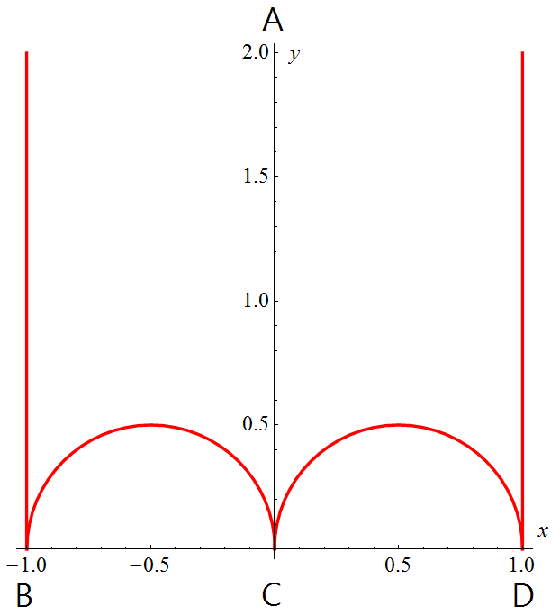
(a) A fundamental polygon $\mathfrak{D}_{\mathbb{H}}$ on the Poincaré half-plane.

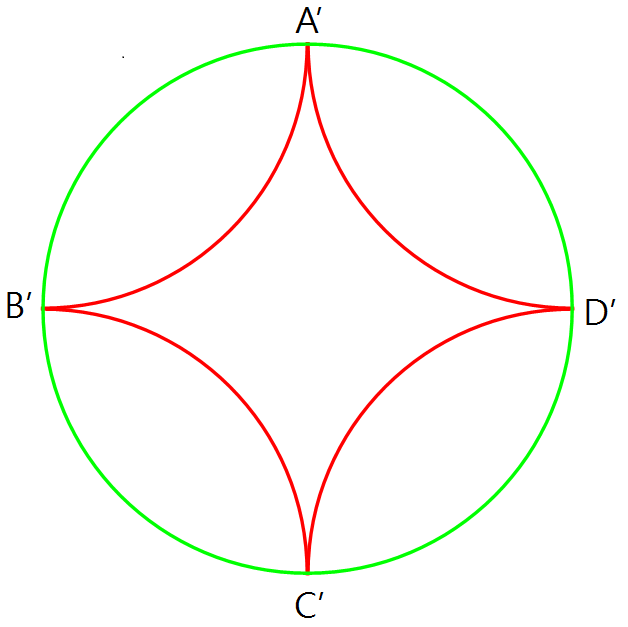
(b) A fundamental polygon $\mathfrak{D}_{\mathbb{D}}$ on the hyperbolic disk.

Figure 22: Fundamental polygons for the uniformization of $Y(2)$ to the Poincaré half-plane and to the hyperbolic disk.

B.2 Local holomorphic cusp coordinates on $Y(2)$

Local holomorphic coordinates $u_{0},u_{1},u_{\infty}$ can be constructed around each of the punctures $\zeta=0,1,\infty$ as explained in (genalpha, , Sec. 5.4):

1. The point $\tau=\infty$ (which projects to $\zeta=0$) is invariant under the action of the cyclic subgroup of $\gamma$ generated by the parabolic element $P_{\infty}$ of (17), which acts as the translation $\tau\rightarrow\tau+2$. The element $T_{\infty}=\left[\begin{array}[]{cc}\frac{1}{\sqrt{2}}&0\\ 0&\sqrt{2}\end{array}\right]\in\mathrm{PSL}(2,\mathbb{R})$ acts as $T_{\infty}\tau=\frac{\tau}{2}$ and satisfies $(T_{\infty}P_{\infty}T_{\infty}^{-1})(\tau)=\tau+1$. Hence the holomorphic cusp coordinate around $\zeta=0$ is given by genalpha :

   $$u_{0}=e^{2\pi\mathbf{i}T_{\infty}\tau}=e^{\mathbf{i}\pi\tau}=e^{\mathbf{i}\pi\mu(\zeta)}~{}~{}.$$

   In the expression above, it is understood that one chooses a branch of the multivalued inverse (18) for which $\tau=\mu(\zeta)$ belongs to the cusp domain:

   $$\mathcal{C}_{\infty}=\{\tau\in\mathbb{H}\,|\,\mathrm{Im}\tau>2\}~{}~{}.$$

   This insures that $u_{0}$ covers the punctured disk $0<|u_{0}|<e^{-2\pi}$ (see genalpha ; elem ).

2. The point $\tau=0$ (which projects to $\zeta=1$) is invariant under the action of the cyclic subgroup of $\Gamma$ generated by the parabolic element $P_{0}$ of (17). The element $T_{0}=\left[\begin{array}[]{cc}0&\frac{1}{\sqrt{2}}\\ -\sqrt{2}&0\end{array}\right]\in\mathrm{PSL}(2,\mathbb{R})$ acts as $T_{0}\tau=-\frac{1}{2\tau}$ and satisfies $(T_{0}P_{\infty}T_{0}^{-1})(\tau)=\tau+1$. Hence the holomorphic cusp coordinate around $\zeta=1$ is given by:

   $$u_{1}=e^{2\pi\mathbf{i}T_{0}\tau}=e^{-\frac{\mathbf{i}\pi}{\tau}}=e^{-\frac{\mathbf{i}\pi}{\mu(\zeta)}}~{}~{}.$$

   In the expression above, one must choose a branch of $\mu$ for which $\tau=\mu(\zeta)$ belongs to the cusp domain:

   $$\mathcal{C}_{0}=\{\tau\in\mathbb{H}\,|\,\mathrm{Im}\frac{1}{\tau}<-2\}=\{\tau\in\mathbb{H}\,|\,\mathrm{Im}\tau>2|\tau|^{2}\}~{}~{}.$$

   This insures that $u_{1}$ covers the punctured disk $0<|u_{1}|<e^{-2\pi}$ .

3. The point $\tau=1$ (which projects to $\zeta=\infty$) is invariant under the action of the cyclic subgroup of $\Gamma$ generated by the parabolic element:

   $$P_{1}\stackrel{{\scriptstyle{\rm def.}}}{{=}}P_{\infty}P_{0}=\left[\begin{array}[]{cc}-3&2\\ -2&1\end{array}\right]~{}~{},$$

   which acts as $P_{1}\tau=\frac{2-3\tau}{1-2\tau}$. The element $T_{1}=\left[\begin{array}[]{cc}0&-\frac{1}{\sqrt{2}}\\ \sqrt{2}&-\sqrt{2}\end{array}\right]\in\mathrm{PSL}(2,\mathbb{R})$ acts as $T_{1}\tau=\frac{1}{2(1-\tau)}$ and satisfies $(T_{1}P_{1}T_{1}^{-1})(\tau)=\tau-1$. Hence the holomorphic cusp coordinate around $\zeta=\infty$ is given by:

   $$u_{\infty}=e^{2\pi\mathbf{i}T_{1}\tau}=e^{\frac{\mathbf{i}\pi}{1-\tau}}=e^{\frac{\mathbf{i}\pi}{1-\mu(\zeta)}}~{}~{}.$$

   In the expression above, one must choose a branch of $\mu$ for which $\tau=\mu(\zeta)$ belongs to the cusp domain:

   $$\mathcal{C}_{1}=\{\tau\in\mathbb{H}\,|\,\mathrm{Im}\left(\frac{1}{1-\tau}\right)>2\}=\{\tau\in\mathbb{H}\,|\,\mathrm{Im}\tau>2|1-\tau|^{2}\}~{}~{}.$$

   This insures that $u_{\infty}$ covers the punctured disk $0<|u_{\infty}|<e^{-2\pi}$.

Let $c\in\{0,1,\infty\}$ be any of the punctures, $u_{c}$ be the local holomorphic cusp coordinate introduced above and $\dot{\mathcal{D}}_{c}$ be the punctured neighborhood of $c$ in $Y(2)$ defined by $0<|u_{c}|<e^{-2\pi}$. The restriction of the hyperbolic metric (16) to $\dot{\mathcal{D}}_{c}$ is given by:

$$\mathrm{d}s^{2}|_{\dot{\mathcal{D}}_{c}}=\Lambda(u_{c},\bar{u}_{c})^{2}|\mathrm{d}u_{c}|^{2}~{}~{},~{}\mathrm{with}~{}~{}\Lambda(u_{c},\bar{u}_{c})=\frac{1}{|u_{c}|\log(1/|u_{c}|)}~{}~{}.$$ (94)

This is the standard form of the hyperbolic cusp metric Borthwick ; elem . It can be brought to the form:

$$\mathrm{d}s^{2}|_{\dot{\mathcal{D}}_{c}}=\mathrm{d}r^{2}+\frac{e^{-2r}}{(2\pi)^{2}}\mathrm{d}\theta^{2}~{}~{}$$ (95)

upon passing to semi-geodesic coordinates $(r_{c},\theta_{c})$ around the puncture $c$ through the transformation elem :

$$u_{c}=e^{2\pi e^{r_{c}}+\mathbf{i}\theta_{c}}~{}~{}.$$

In these coordinates, the puncture $c$ is located at $r_{c}\rightarrow+\infty$ and $\theta$ runs from $0$ to $2\pi$.

References

• (1) C. I. Lazaroiu, C. S. Shahbazi, Generalized two-field $\alpha$-attractor models from geometrically finite hyperbolic surfaces, Nuclear Physics. B, Vol. 936 (2018), 542-596, https://doi.org/10.1016/j.nuclphysb.2018.09.018.
• (2) C. M. Peterson, M. Tegmark, Testing Two-Field Inflation, Phys. Rev. D 83 (2011) 023522, arXiv:1005.4056 [astro-ph.CO].
• (3) C. M. Peterson, M. Tegmark, Non-Gaussianity in Two-Field Inflation, Phys. Rev. D 84 (2011) 023520, arXiv:1011.6675 [astro-ph.CO].
• (4) C. Gordon, D. Wands, B. A. Bassett, R. Maartens, Adiabatic and entropy perturbations from inflation, Phys. Rev D 63 (2001) 023506, astro-ph/0009131.
• (5) S. G. Nibbelink, B. van Tent, Scalar perturbations during multiple field slow-roll inflation Class. Quant. Grav. 19 (2002) 613–640, hep-ph/0107272.
• (6) Z. Lalak, D. Langlois, S. Pokorski, K. Turzynski, Curvature and isocurvature perturbations in two-field inflation, JCAP 0707 (2007) 014, arXiv:0704.0212 [hep-th].
• (7) S. Cremonini, Z. Lalak, K. Turzynski, Strongly Coupled Perturbations in Two-Field Inflationary Models, JCAP, 1103 (2011) 016, arXiv:1010.3021 [hep-th].
• (8) A. Achucarro, J.-O. Gong, S. Hardeman, G. A. Palma, S. P. Patil, Features of heavy physics in the CMB power spectrum, JCAP 1101 (2011) 030, arXiv:1010.3693 [hep-ph].
• (9) A. Achucarro, J.-O. Gong, S. Hardeman, G. A. Palma, S. P. Patil, Mass hierarchies and nondecoupling in multi-scalar field dynamics, Phys. Rev. D 84 (2011) 043502, arXiv:1005.3848 [hep-th].
• (10) J.-O. Gong, Multi-field inflation and cosmological perturbations,Int. J. Mod. Phys D 26 (2017) 1, 1740003, arXiv:1606.06971 [gr-qc].
• (11) R. Schimmrigk, Automorphic inflation, Phys. Lett. B 748 (2015) 376, arXiv: 1412.8537 [hep-th].
• (12) R. Schimmrigk, A geneneral framework of automorphic inflation, JHEP 05 (2016) 140, arXiv: 1512.09082 [hep-th].
• (13) R. Schimmrigk, Modular inflation observables and j-inflation phenomenology, JHEP09 (2017) 043, arXiv:1612.09559 [hep-th].
• (14) R. Schrimmrigk, Multifield Reheating after Modular j-Inflation, arXiv:1712.09961 [hep-ph].
• (15) M. Dias, J. Frazer, D. Seery, Computing observables in curved multifield models of inflation – A guide (with code) to the transport method, JCAP 12 (2015) 030.
• (16) M. Dias, J. Frazer, D. J. Mulryne, D. Seery, Numerical evaluation of the bispectrum in multiple field inflation, JCAP 12 (2016) 033.
• (17) D. J. Mulryne, PyTransport: A Python package for the calculation of inflationary correlation functions, arXiv:1609.00381 [astro-ph.CO].
• (18) K. Kainulainen, J. Leskinen, S. Nurmi, T. Takahashi, CMB spectral distortions in generic two-field models, JCAP 11 (2017) 002 [astro-ph.CO].
• (19) N. Bartolo, D.M.Bianco, R. Jimenez, S. Matarrese, L. Verde. Supergravity, $\alpha$-attractors and primordial non-Gaussianity, arXiv:1805.04269 [astro-ph.CO].
• (20) P. A. R. Ade et al. [Planck Collaboration], Astron. Astrophys. 594 (2016) A20, arXiv:1502.02114 [astro-ph.CO].
• (21) J. J. M. Carrasco, R. Kallosh, A. Linde, D. Roest, The hyperbolic geometry of cosmological attractors, Phys. Rev. D 92 (2015) 4, 41301, arXiv:1504.05557 [hep-th].
• (22) R. Kallosh, A. Linde, Escher in the Sky, Comptes Rendus Physique 16 (2015) 914, arXiv:1503.06785 [hep-th].
• (23) R. Kallosh, A. Linde, D. Roest, A universal attractor for inflation at strong coupling, Phys. Rev. Lett. 112 (2014) 011303, arXiv:1310.3950 [hep-th].
• (24) M. Galante, R. Kallosh, A. Linde, D. Roest, The Unity of Cosmological Attractors, Phys. Rev. Lett. 114 (2015) 141302, arXiv:1412.3797 [hep-th].
• (25) H. P. de Saint-Gervais, Uniformization of Riemann Surfaces: revisiting a hundred-year-old theorem, EMS Heritage of European Mathematics, Vol. 11 (2016) 512 pp.
• (26) S. Katok, Fuchsian Groups, U. Chicago Press, 1992.
• (27) A. F. Beardon, The geometry of discrete groups, Graduate Texts in Mathematics 91, Springer, 1983.
• (28) W. Fenchel, J. Nielsen, Discontinuous Groups of Isometries in the Hyperbolic Plane, De Gruyter, 2003.
• (29) E. M. Babalic, C. I. Lazaroiu, Generalized $\alpha$-attractor models from elementary hyperbolic surfaces, Adv. Math. Phys. 2018 (2018), Art. ID 7323090.
• (30) D. Borthwick, Spectral Theory of Infinite-Area Hyperbolic Surfaces, Progr. in Math. 256, Birkhäuser, Boston, 2007.
• (31) F. Diamond, J. Shurman, A First Course in Modular Forms, Graduate Texts in Mathematics, Springer, 2005.
• (32) G. Shimura, Introduction to the Arithmetic Theory of Automorphic Functions, Princeton U.P., 1971.
• (33) L. V. Ahlfors, Complex analysis (3rd ed.), Mc. Graw-Hill, 1979.
• (34) I. Richards, On the Classification of Non-Compact Surfaces, Transactions of the AMS 106 (1963) 2, 259–269.
• (35) S. Stoilow, Leçons sur les principes topologiques de la théorie des fonctions analytiques, Gauthier-Villars, Paris, 1956.
• (36) A. Haas, Linearization and mappings onto pseudocircle domains, Trans. Amer. Math. Soc. 282 (1984), 415–429.
• (37) B. Maskit, Canonical domains on Riemann surfaces, Proc. Amer. Math. Soc. 106 (1989), 713–721.
• (38) S. Agard, Distortion theorems for quasiconformal mappings. Ann. Acad. Sci. Fenn. A I Math. 413 (1968) 1–12.
• (39) A . Yu. Solynin, M. Vuorinen, Estimates for the hyperbolic metric of the punctured plane and applications, Israeli Journal of Mathematics 124 (2001) 29–60.
• (40) T. Sugawa, M. Vuorinen, Some inequalities for the Poincaré metric of plane domains, Math. Z. 250 (2005) 4, 885–906.
• (41) S. Zemel, Normalizers of Congruence Groups in $SL_{2}(\mathbb{R})$ and Automorphisms of Lattices, arXiv:1512.07547 [math.NT].
• (42) M. Newman, Normalizers of Modular Groups, Math. Ann. 238 (1978) 2, 123–129.
• (43) R. Hain, Lectures on moduli spaces of elliptic curves, pp. 95–166 in “Transformation groups and moduli spaces of curves” (eds. L. Ji, S.-T. Yau), Adv. Lectures in Math. 16, International Press, 2011.
• (44) A. Sebbar, Torsion-free genus zero congruence subgroups of $\mathrm{PSL}_{2}(\mathbb{R})$, Duke Math. J. 110 (2001) 2.
• (45) S. Hellerman, E. Sharpe, Sums over topological sectors and quantization of Fayet-Iliopoulos parameters, Adv. Theor. Math. Phys. 15 (2011) 1141–1199, arXiv:1012.5999 [hep-th].
• (46) T. Banks, N. Seiberg Symmetries and Strings in Field Theory and Gravity, Phys.Rev. D 83 (2011) 084019, arXiv:1011.5120 [hep-th].
• (47) P. G. Camara, L. E. Ibanez, F. Marchesano, RR photons, JHEP 09 (2011) 110, arXiv:1106.0060 [hep-th].
• (48) M. Berasaluce-Gonzalez, P. G. Camara, F. Marchesano, D. Regalado, A. M. Uranga, Non-Abelian discrete gauge symmetries in 4d string models, JHEP 09 (2012) 059, arXiv:1206.2383 [hep-th].
• (49) F. Marchesano, G. Shiu, A. M. Uranga, F-term Axion Monodromy Inflation, JHEP 09 (2014) 184, arXiv:1404.3040 [hep-th].