Energy Efficient Precoding C-RAN Downlink with Compression at Fronthaul

Abstract

This paper considers a downlink transmission of cloud radio access network (C-RAN) in which precoded baseband signals at a common baseband unit are compressed before being forwarded to radio units (RUs) through limited fronthaul capacity links. We investigate the joint design of precoding, multivariate compression and RU-user selection which maximizes the energy efficiency of downlink C-RAN networks. The considered problem is inherently a rank-constrained mixed Boolean nonconvex program for which a globally optimal solution is difficult and computationally expensive to find. In order to derive practically appealing solutions, we invoke some useful relaxation and transformation techniques to arrive at a more tractable (but still nonconvex) continuous program. To solve the relaxation problem, we propose an iterative procedure based on DC algorithms which is provably convergent. Numerical results demonstrate the superior of the proposed solution in terms of achievable energy efficiency compared to existing schemes.

I Introduction

The evolution of wireless communication techniques towards the foreseen fifth generation (5G) wireless networks envisions a dramatic growth of wireless devices, applications and demand on wireless data traffic [1, 2]. Accordingly, spectral efficiency (SE) will certainly play a major role in future cellular. As well concluded in pioneer research, multicell cooperation or cooperative multipoint processing (CoMP) with joint base station (BS) processing and transmission is a promising enabling technique to tackle the ‘spectrum crunch’ problem [3, 4]. However, the transmission with large numbers of antenna elements consumes remarkable amount of processing power or energy. Thus energy-efficiency (EE) has appeared as another important design objective. Recently, energy-efficient techniques and architectures for cooperative transmission have been intensively investigated [5].

Among them, cloud radio access network (C-RAN) is appearing as a revolutionary architectural solution to the problem of enhanced SE and EE requirements for cellular networks [5, 6]. In CRANs, baseband (BB) signal processing components are no longer deployed at base stations, but installed at a common BB unit (BBU), which is now responsible for the encoding/decoding and other computational tasks on transmitted signals. Thus CRANs can take full advantage of the cooperative principle to boost the achievable SE. In addition, conventional BSs are also replaced by low-cost low-power ones which are equipped with only radio frequency modules, thereby reducing the power cost for management and operating the BSs. Such a BS is often called as radio unit (RU). Nevertheless, to perform the transmission/reception, each RU has to receive/forward BB signals from/to the BBU through fronthaul links, which can be wired or wireless. In either case, they are capacity limited and thus allow only a limited amount of BB information to be transferred per a time unit. This limitation explicitly restricts the performance of C-RANs and becomes a factor that needs to be taken into consideration in the system design [7].

This paper is focused on the downlink transmission of C-RAN such that the BB signals are precoded at the BBU, which are then compressed before being forwarded to RUs through fronthaul links. We aim at studying a joint design of precoding, multivariate compression and RU-user selection that maximizes the EE of the CRAN downlink under a limited power budget and finite-capacity fronthaul links. More specifically, joint precoding and multivariate compression design are adopted to improve the system throughput [8, 9], while a proper RU-user selection scheme potentially reduces the power and fronthaul expenditure of the network. The considered problem is cast as a rank-constrained mix-Boolean nonconvex program, which belongs to a class of NP-hard problems, and thus a globally optimal solution is hard to find. Therefore, we propose a low-complexity method that solves the problem locally, which is a classical goal for such an NP hard problem. To this purpose, we first drop the rank constraint and lift the Boolean variables into the continuous domain. Then by using novel transformations, we show that the relaxed problem admits a difference of convex (DC) function structure, which motivates the application of DC algorithms [10, 11, 12] to achieve suboptimal solutions. Particularly, the problem is convexified into a semidefinite program (SDP) at each iteration of the proposed algorithm using the principle of the DC programming. This produces a sequence of iterates which provably converges to a stationary point, i.e., fulfilling the Karush-Kuhn-Tucker (KKT) optimality conditions of the relaxed problem. Numerical experiments are carried out to evaluate the proposed algorithm.

II System Model and Problem Formulation

II-A System Models

Consider a multiple-input single-output (MISO) downlink transmission of C-RAN where several low-cost low-power RUs serve multiple single-antenna users. Each RU is equipped with $M$ antennas. Let us denote by $B$ and $K$ the number of RUs and users in the network, respectively. We assume that all RUs are connected to a common BBU through finite-capacity fronthaul links. The BBU is also assumed to have all users’ data and (perfect) channel state information (CSI). We consider a fronthaul network with compression strategy where BB signals for transmission are precoded and compressed at the BBU before being forwarded to RUs. Let $\{s_{k}\}_{k=1}^{K}$ be a set of the intended data to users in which $s_{k}$ is a Gaussian input with unit energy, i.e., $\mathbb{E}[|s_{k}|^{2}]=1$. Suppose that linear precoding is adopted at the BBU. The BB signal generated for the transmission at RU $b$ is written as

$${\bf x}_{b}=\sum_{k=1}^{K}{\bf w}_{b,k}s_{k}$$ (1)

where ${\bf w}_{b,k}\in\mathbb{C}^{M\times 1}$ is the beamformer from RU $b$ to user $k$. ${\bf x}_{b}$ is then compressed and forwarded to RU $b$ through the fronthaul link. We assume that the Gaussian test channel is used to model the effect of compression on the fronthaul link [9]. Accordingly, the BB signal at RU $b$ is given by

$$\hat{{\bf x}}_{b}={\bf x}_{b}+{\bf q}_{b}$$ (2)

where ${\bf q}_{b}\in\mathbb{C}^{M\times 1}$ is the quantization noise, which is independent of ${\bf x}_{b}$, and modeled as a complex Gaussian distribution vector with covariance ${\bf Q}_{b,b}$, i.e., ${\bf q}_{b}\sim\mathcal{CN}(0,{\bf Q}_{b,b})$. Note that ${\bf Q}_{b,b}$ is full-rank, i.e., $\text{rank}({\bf Q}_{b,b})=M$. We further assume so called multivariate compression such that the compression of BB signals for each RU is mutually dependent. Thus the associated quantization noise vectors are correlated, i.e., ${\bf Q}_{b,i}=\mathbb{E}[{\bf q}_{b}{\bf q}_{i}^{H}]\neq 0,\forall b\neq i$. Based on the information theoretic formulation [13, Ch. 9], RU $b$ can successfully receive $\hat{{\bf x}}_{b}$ as long as the following condition holds

$$\sum_{b=1}^{B}\log\left|{\bf Q}_{b,b}+\sum_{k=1}^{K}{\bf w}_{b,k}{\bf w}_{b,k}^{H}\right|-\log\left|{\bf Q}\right|\leq\sum_{b=1}^{B}\bar{C}_{b}$$ (3)

where

$${\bf Q}\triangleq\left[\begin{array}[]{cccc}{\bf Q}_{1,1}&{\bf Q}_{1,2}&\cdots&{\bf Q}_{1,B}\\ {\bf Q}_{2,1}&{\bf Q}_{2,2}&&{\bf Q}_{2,B}\\ \vdots&&\ddots&\vdots\\ {\bf Q}_{B,1}&{\bf Q}_{B,2}&\cdots&{\bf Q}_{B,B}\end{array}\right]$$

is the compression covariance matrix and $\bar{C}_{b}$ is the capacity of the frontlink between BBU and RU $b$. At RU $b,$ the BB signal $\hat{{\bf x}}_{b}$ is transmitted to users through flat fading channels. The received signal of user $k$ can be written as

$$y_{k} =\sum_{b=1}^{K}{\bf h}_{b,k}\hat{{\bf x}}_{b}+\sigma_{k}=\sum_{b=1}^{B}{\bf h}_{b,k}(\sum_{k=1}^{K}{\bf w}_{b,k}s_{k}+{\bf{\bf q}}_{b})+\sigma_{k}$$

$$={\bf h}_{k}{\bf w}_{k}+\sum_{j\neq k}^{K}{\bf h}_{k}{\bf w}_{j}+\sum_{b=1}^{B}{\bf h}_{b,k}{\bf q}_{b}+\sigma_{k}$$ (4)

where ${\bf h}_{b,k}\in\mathbb{C}^{1\times M}$ is the (row) vector representing the channel between RU $b$ and user $k$, and $\sigma_{k}\sim\mathcal{CN}(0,N_{0})$ is the additive white Gaussian noise at user $k$. In (4), ${\bf h}_{k}\triangleq[{\bf h}_{1,k},{\bf h}_{2,k},\ldots,{\bf h}_{B,k}]\in\mathbb{C}^{1\times MB}$ and ${\bf w}_{k}\triangleq[{\bf w}_{1,k}^{T},{\bf w}_{2,k}^{T},\ldots,{\bf w}_{B,k}^{T}]^{T}$ $\in\mathbb{C}^{MB\times 1}$ denote the aggregate vectors of channels and beamformers from all RUs to user $k$, respectively. We also denote ${\bf W}_{k}\triangleq{\bf w}_{k}{\bf w}_{k}^{H}\succeq 0$, ${\bf W}_{k}\in\mathbb{C}^{MB\times MB}$, $\text{rank}({\bf W}_{k})=1,\forall k$ and ${\bf w}_{b,k}{\bf w}_{b,k}^{H}={\bf T}_{b}{\bf W}_{k}{\bf T}_{b}^{T}$ where ${\bf T}_{b}\in\mathbb{R}_{+}^{M\times MB}$ is all-zero matrix except the columns from $((b-1)M+1)$ to $(bM)$ which contain the identity matrix. Suppose that single-user decoding is used and the intercell-interference is treated as Gaussian noise. By the multivariate compression strategy, the achievable rate for user $k$ is given by [13, Ch. 9]

$$r_{k}({\bf W},{\bf Q})\triangleq$$ (5)

$$W\log\left(1+\frac{{\bf h}_{k}{\bf W}_{k}{\bf h}_{k}^{H}}{{\textstyle\sum_{j\neq k}^{K}}{\bf h}_{k}{\bf W}_{j}{\bf h}_{k}^{H}+{\bf h}_{k}{\bf Q}{\bf h}_{k}^{H}+WN_{0}}\right)$$

where $W$ is the bandwidth.

II-B RU-user Selection Scheme

We can see from (3) and (5) that there is a trade-off among power of the beamformers, quantization noise covariances, and users’ throughput under the finite-capacity fronthaul links. More specifically, due to the constraint in (3), it is not always possible to increase SE simply by using more transmit power and/or making quantization noise variances small [9]. Therefore, we propose to employ an RU-user selection scheme where each user is only served by neighboring RUs of significant strength. The idea is that the power consumption are saved while diversity provided by multicell cooperation is still exploited to increase the transmission quality. In the selection scheme, beamformers between a BS and a user is made to be zero if the corresponding link is not selected. Mathematically, let us denote by $\phi_{b,k}\in\{0,1\}$ the selection preference variable where $\phi_{b,k}=1$ indicates that RU $b$ serves user $k$ and $\phi_{b,k}=0$ otherwise. The relation between beamformer ${\bf w}_{b,k}$ and variable $\phi_{b,k}$ is given by $\text{tr}({\bf T}_{b}{\bf W}_{k}{\bf T}_{b}^{T})\leq\phi_{b,k}u_{b,k}$ where $u_{b,k}$ is subject to a considered power constraint. Obviously, $\phi_{b,k}=0$ implies ${\bf w}_{b,k}=0$.

II-C Power Consumption Model

Besides the data-dependent power consumption which is due to the BB signal generation, i.e., $P_{\text{data}}\triangleq\frac{1}{\epsilon}(\sum_{b=1}^{B}\sum_{k=1}^{K}\text{tr}({\bf T}_{b}{\bf W}_{k}{\bf T}_{b}^{T})+\sum_{b=1}^{B}\text{tr}({\bf Q}_{b,b}))$ (where $\epsilon$ is power amplifier efficiency), we need to consider all other sources of power which are spent for the network operation. Those are generally referred as data-independent power consumption which consists of the power consumed by operating the signal processing circuits at the BBU, RUs, users and the fronthaul network, i.e.,

$$P_{0}\triangleq\sum_{b=1}^{B}\sum_{k=1}^{K}\phi_{b,k}P_{b,k}^{\text{cir}}+KP_{\text{Us}}+BP_{\text{RU}}$$ (6)

where $P_{b,k}^{\text{cir}}$ is power for signal processing circuit block of beamformer ${\bf w}_{b,k}$; $P_{\text{RU}}$ denotes the circuit power consumed at an RU; and $P_{\text{Us}}$ is the circuit power of a user.

II-D Problem Formulation

We are interested in a joint design of precoding, multivariate compression and RU-user link selection that maximizes the network EE subject the limited fronthaul capacity and per-RU power constraints, which is formulated as

$$\underset{{\bf W},{\bf Q},\bm{\phi},{\bf u}}{\max}\ \ f_{\text{EE}}\triangleq\frac{\sum_{k=1}^{K}r_{k}({\bf W},{\bf Q})}{P_{\text{data}}+P_{0}}$$ (7a)

s.t. $$\text{tr}({\bf T}_{b}{\bf W}_{k}{\bf T}_{b}^{T})\leq\phi_{b,k}u_{b,k},\ \forall b,k$$ (7b)

$$\sum_{k=1}^{K}u_{b,k}+\text{tr}({\bf Q}_{b,b})\leq\bar{P},\ \forall b$$ (7c)

$$\sum_{b=1}^{B}\phi_{b,k}\geq 1,\ \forall b,k$$ (7d)

$$\phi_{b,k}\in\{0,1\},\ \forall b,k,$$ (7e)

$$\begin{aligned} &\sum_{b=1}^{B}\log\left|{\bf Q}_{b,b}+\sum_{k=1}^{K}{\bf T}_{b}{\bf W}_{k}{\bf T}_{b}^{T}\right|\\ &\qquad\qquad\qquad\qquad-\log\left|{\bf Q}\right|\leq\sum_{b=1}^{B}\bar{C}_{b}\end{aligned}$$ (7f)

$${\bf W}_{k}\succeq 0,\ \forall k$$ (7g)

$$\text{rank}({\bf W}_{k})=1,\ \text{rank}({\bf Q}_{b,b})=M,\ \forall b,k$$ (7h)

where $\bm{\phi}\triangleq[\phi_{1,k},\ldots\phi_{b,k},\ldots,\phi_{B,K}]\in\{0,1\}^{BK}$. Herein, (7c) is the power constraint with the power budget $\bar{P}$ at RU $b$. (7d) is added to ensure that each user is always served by at least one RU. Clearly, problem (7) is classified as rank-constrained mixed Boolean nonconvex program for which a global optimum is challenging to derive. Thus, a low-complexity solution is more preferable in practice. Toward this end, we drop the rank constraint (7h) and base our proposed solution on the relaxed problem of (7). It is worth mentioning that problem (7) without the rank constraints is still nonconvex and thus intractable.

III Proposed Solution

We now propose an algorithm that finds a suboptimal solution of the rank-relaxed problem of (7) based on the combination of the SDP and DC programming, referred to as the SDP-DC algorithm. In particular, the principle of the DC algorithm is used to iteratively convexify the nonconvexity of the relaxed problem to achieve a sequence of SDP formulations, whose solutions converge to a stationary point of the rank-relaxed problem. To proceed, we note that the Boolean constraint (7e) can be equivalently rewritten as

$$\sum_{b=1}^{B}\sum_{k=1}^{K}(\phi_{b,k}^{2}-\phi_{b,k})\geq 0,\ \phi_{b,k}\in[0,1].$$ (8)

It is easy to see that (8) actually implies that $\phi_{b,k}\in\{0,1\}$. On the other hand, the objective of (7) is a generic fractional function. To arrive at a tractable formulation of the rank relaxed problem of (7), we use the epigraph form to rewrite it as [14]

$$\max_{\begin{subarray}{c}{\bf W},{\bf Q},{\bf u},\bm{\phi},\\ \eta,t,{\bf z},{\bf g},{\bf q}\end{subarray}} \quad\eta$$ (9a)

s. t. $$t\eta\leq\sum_{k=1}^{K}z_{k}$$ (9b)

$$z_{k}\leq\log(1+g_{k})$$ (9c)

$$\begin{aligned} t\geq&\sum_{b=1}^{B}\sum_{k=1}^{K}(\frac{1}{\epsilon}u_{b,k}+\phi_{b,k}P_{b,k}^{\text{cir}})+KP_{\text{Us}}\\ &\qquad\qquad\qquad+BP_{\text{RU}}+\frac{1}{\epsilon}\sum_{b=1}^{B}\text{tr}({\bf Q}_{b,b})\end{aligned}$$ (9d)

$$g_{k}q_{k}\leq{\bf h}_{k}{\bf W}_{k}{\bf h}_{k}^{H}$$ (9e)

$$q_{k}\geq\sum_{j\neq k}^{K}{\bf h}_{k}{\bf W}_{j}{\bf h}_{k}^{H}+{\bf h}_{k}{\bf Q}{\bf h}_{k}^{H}+WN_{0}$$ (9f)

$$\eqref{eq:soft power:precoder},\eqref{eq:power},\eqref{eq:min:connectivity},\eqref{eq:BH:constraint-1},\eqref{eq:PSD},\eqref{eq:boolean:relax}$$ (9g)

where ${\bf z}=[z_{1},\ldots,z_{K}]$, ${\bf g}=[g_{1},\ldots,g_{K}]$ and ${\bf q}=[q_{1},\ldots,q_{K}]$. Further, in light of DC programming (or concave-convex procedure), we rewrite (7b), (9b) and (9e) as

$$(\phi_{b,k}-u_{b,k})^{2} \leq(\phi_{b,k}+u_{b,k})^{2}-4\text{tr}({\bf T}_{b}{\bf W}_{k}{\bf T}_{b}^{T})$$ (10)

$$(\eta+t)^{2} \leq(\eta-t)^{2}+4\sum_{k=1}^{K}z_{k}$$ (11)

$$(g_{k}+q_{k})^{2} \leq(g_{k}-q_{k})^{2}+4{\bf h}_{k}{\bf W}_{k}{\bf h}_{k}^{H}$$ (12)

where the functions in both sides of the above constraints are convex, which are amendable for the application of the DC algorithm. However, direct applying DC algorithm to (9) always results in an infeasible program. To understand this, let us recall constraint (8) and replace the term $\phi_{b,k}^{2}$ by its linear approximation at feasible point $\hat{\phi}_{b,k}\in\{0,1\}$ according to the DC algorithm, i.e.,

$$\Phi(\bm{\phi},\hat{\bm{\phi}})\triangleq\sum_{b=1}^{B}\sum_{k=1}^{K}(2\phi_{b,k}\hat{\phi}_{b,k}-(\hat{\phi}_{b,k})^{2}-\phi_{b,k})\geq 0.$$ (13)

It is not difficult to check that the set $\{\phi_{b,k}\in[0,1]|\Phi(\bm{\phi},\tilde{\bm{\phi}})>0\}$ is empty. To cope with this issue, we apply a regularization technique to arrive at the following program

$$\max_{\begin{subarray}{c}{\bf W},{\bf Q},{\bf u},\bm{\phi},\eta,t,{\bf z},{\bf g},{\bf q},\lambda\end{subarray}} \quad\eta-\alpha\lambda$$ (14a)

s. t. $$\lambda+\sum_{b=1}^{B}\sum_{k=1}^{K}(\phi_{b,k}^{2}-\phi_{b,k})\geq 0$$ (14b)

$$\eqref{eq:power},\eqref{eq:min:connectivity},\eqref{eq:BH:constraint-1},\eqref{eq:PSD},\eqref{eq:rate:epi},\eqref{eq:power:consumption:epi},\eqref{eq:infererence:epi},$$ (14c)

$$\eqref{eq:soft-pow-precoder:rewrite},\eqref{eq:EE:epi:rewrite},\eqref{eq:SINR:epi:rewrite}$$ (14d)

by adding a slack variable $\lambda\geq 0$ and a penalty parameter $\alpha$. As can be seen, $\lambda$ allows (13) to be satisfied for any $\hat{\phi}_{b,k}\in[0,1]$. In addition, $\lambda$ is to be minimized in (14) and $\lambda=0$ immediately implies that an optimal solution of (14) is also feasible to (9).

We are now ready to propose a novel iterative algorithm that solves (14). The central idea of the method is to linearize the nonconvex parts of (7f), (10)–(12) and (14b) at each iteration to produce a sequence of solutions that converge to a stationary point. Mathematical justification of the proposed iterative approach is given in the following where the superscript denotes the iteration index. We begin with the constraints in (10)–(12) which all have the same form $(x+y)^{2}+w$ of which a convex lower bound is simply given by $2(x^{(n)}+y^{(n)})(x+y)-(x^{(n)}+y^{(n)})^{2}+w$ for any operating point $x^{(n)}$ and $y^{(n)}$. Thus, we can approximate (10)–(12) by the following second order cone constraints

$$\begin{aligned} &(\phi_{b,k}-u_{b,k})^{2}\leq 2(\phi_{b,k}^{(n)}+u_{b,k}^{(n)})(\phi_{b,k}+u_{b,k})\\ &\qquad\qquad\qquad\quad-(\phi_{b,k}^{(n)}+u_{b,k}^{(n)})^{2}-4\text{tr}({\bf T}_{b}{\bf W}_{k}{\bf T}_{b}^{T})\end{aligned}$$ (15)

$$\begin{aligned} &(\eta+t)^{2}\leq 2(\eta^{(n)}-t^{(n)})(\eta-t)\\ &\qquad\qquad\qquad\quad-(\eta^{(n)}-t^{(n)})^{2}+4\sum_{k=1}^{K}z_{k}\end{aligned}$$ (16)

$$\begin{aligned} &(g_{k}+q_{k})^{2}\leq 2(g_{k}^{(n)}-q_{k}^{(n)})(g_{k}-q_{k})\\ &\qquad\qquad\qquad\quad-(g_{k}^{(n)}-q_{k}^{(n)})^{2}+4{\bf h}_{k}{\bf W}_{k}{\bf h}_{k}^{H}.\end{aligned}$$ (17)

In the same manner, (14b) can be replaced by

$$\lambda+\Phi(\bm{\phi},\bm{\phi}^{(n)})\geq 0$$ (18)

Now we turn our attention to the remaining nonconvex constraint (7f) and denote $h_{b}({\bf W},{\bf Q})\triangleq\log|{\bf Q}_{b,b}+\sum_{k=1}^{K}{\bf T}_{b}{\bf W}_{k}{\bf T}_{b}^{T}|$. Remark that $h_{b}({\bf W},{\bf Q})$ is jointly concave and differentiable w.r.t. ${\bf W}$ and ${\bf Q}$ in domain $\{{\bf W},{\bf Q}\ |\ {\bf W}\succeq 0,{\bf Q}\succeq 0\}$. This allows us for deriving the affine majorization of $h_{b}({\bf W},{\bf Q})$ [15, 8], i.e.,

$$h_{b}^{(n)}({\bf W},{\bf Q};{\bf W}^{(n)},{\bf Q}^{(n)})\triangleq h_{b}({\bf W}^{(n)},{\bf Q}^{(n)})+$$

$$\sum_{k=1}^{K}\text{tr}({\bf T}_{b}^{T}({\bf T}_{b}(\sum_{k=1}^{K}{\bf W}_{k}^{(n)}){\bf T}_{b}^{T}+{\bf Q}_{b,b}^{(n)})^{-1}{\bf T}_{b}({\bf W}_{k}-{\bf W}_{k}^{(n)}))$$

$$+\text{tr}(({\bf T}_{b}({\textstyle\sum_{k=1}^{K}}{\bf W}_{k}^{(n)}){\bf T}_{b}^{T}+{\bf Q}_{b,b}^{(n)})^{-1}({\bf Q}_{b,b}-{\bf Q}_{b,b}^{(n)}))$$

which is the upper bound of $h_{b}({\bf W},{\bf Q})$, i.e., $h_{b}^{(n)}({\bf W},{\bf Q};{\bf W}^{(n)},{\bf Q}^{(n)})\geq h_{b}({\bf W},{\bf Q})$. Again in the light of DC algorithm, (7f) can be replaced by the convex constraint

$$\sum_{b=1}^{B}h_{b}^{(n)}({\bf W},{\bf Q};{\bf W}^{(n)},{\bf Q}^{(n)})-\log|{\bf Q}|\leq\sum_{b=1}^{B}\bar{C}_{b}.$$ (19)

Finally, problem (14) at iteration $n+1$ of the proposed algorithm is approximated by the following convex program

$$\max_{{\bf s}}\ \eta-\alpha^{(n)}\lambda\ \text{s.t.} \{\eqref{eq:power},\eqref{eq:min:connectivity},\eqref{eq:PSD},\eqref{eq:rate:epi},\eqref{eq:power:consumption:epi},\eqref{eq:infererence:epi},$$ (20)

$$\ \ \ \ \eqref{eq:pow:precoderi:approx},\eqref{eq:EE:epi:approx},\eqref{eq:SINR:epi:approx},\eqref{eq:phi:relax:approx},\eqref{eq:BH:approx}\}$$

where ${\bf s}\triangleq\{{\bf W},{\bf Q},{\bf u},\bm{\phi},\eta,t,{\bf z},{\bf g},{\bf q},\lambda\}$ denotes all the optimization variables. The proposed method is summarized in Algorithm 1. In particular, the value of penalty parameter $\alpha$ is not a constant in Algorithm 1 and the update of $\alpha$ (see step 5) at each iteration deserves some comments. In fact, $\alpha$ relates to the degree of relaxation in (20), i.e., a large $\alpha$ strongly forces $\lambda\rightarrow 0$ leading to $\phi_{b,k}\in\{0,1\}$, which implies more tightness for the selection variable $\phi_{b,k}$ and vice versa. Thus, we initialize $\alpha^{(0)}$ by a small value to provide more searching space for $\bm{\phi}$, and then gradually increase $\alpha$ with a factor $c>1$ until $\|\bm{\phi}^{(n+1)}-\bm{\phi}^{(n)}\|_{2}$ is small enough. This update rule provably ensures that $\alpha^{(n)}$ is bounded and $\underset{n\rightarrow+\infty}{\lim}\lambda^{(n)}=0$ as proved in Theorem 1. Another observation is that if Algorithm 1 outputs ${\bf W}^{\ast}$ and ${\bf Q}^{\ast}$ satisfying $\text{rank}({\bf W}^{\ast})=1$ and $\text{rank}({\bf Q}_{b,b}^{\ast})=M$, then ${\bf W}^{\ast}$ and ${\bf Q}^{\ast}$ are also feasible to (7). Since Algorithm 1 is derived on the rank-relaxed problem, it is highly likely that ${\bf Q}^{\ast}$ is full rank matrix. Also, we can prove that Algorithm 1 achieves the rank-1 solution of ${\bf W}_{k}^{\ast}$, but the detailed proof is omitted due to the space limitation. The main idea of the proof is briefly sketched as follows. We derive the dual problem of (20) and show that the Lagrangian multiplier corresponding to ${\bf W}_{k}\succeq 0$ (denoted by ${\bf Z}_{k}$) holds $\text{rank}({\bf Z}_{k})\geq MB-1$. Then by the KKT condition ${\bf Z}_{k}{\bf W}_{k}^{\ast}=0$, we arrive at $\text{rank}({\bf W}^{\ast})=1$. The convergence of Algorithm 1 is studied in the following theorem.

Theorem 1.

There exists a finite positive integer $n_{0}$ such that $\alpha^{(n)}=\alpha^{(n_{0})}$ for $n\geq n_{0}$, i.e., the sequence $\{\alpha^{(n)}\}$ is bounded above and $\underset{n\rightarrow+\infty}{\lim}\lambda^{(n)}=0$. In addition, Algorithm 1 generates a sequence of solutions converging to a stationary point, i.e., fulfilling the KKT optimality conditions of problem (20).

The proof of Theorem 1 is deferred to the Appendix. Since $\underset{n\rightarrow+\infty}{\lim}\lambda^{(n)}=0$, the selection variables converge to binary values eventually, and thus the solution of Algorithm 1 also satisfies the KKT conditions of (9).

Implementation Issues

Algorithm 1 The proposed SDP-DC to solve (20)

1:  Initialization: set $n:=0$, generate a set of initial feasible value ${\bf s}^{(0)}$ of (20) and initial penalty parameter $\alpha^{(0)}$.

2:  repeat

3:     Solve (20) to obtain the set of optimal values ${\bf s}^{\ast}$.

4:     Form the problem for the next iteration with ${\bf s}^{(n+1)}={\bf s}^{\ast}$

5:     Update $\alpha^{(n+1)}:=c\alpha^{(n)}$ if $\|\bm{\phi}^{(n+1)}-\bm{\phi}^{(n)}\|_{2}>\varepsilon$.

6:     $n:=n+1$

7:  until Convergence

8:  Obtain ${\bf W}^{\ast},{\bf Q}^{\ast},\bm{\phi}^{\ast},\eta^{\ast}$.

We now discuss on some practical issues when implementing Algorithm 1. As can be seen, convex program (20) is classified as generic SDP due to the nonlinear constraints (9c) and (19), and thus requires a high computational complexity to solve. To obtain more computationally efficient formulations, we can approximately convert (9c) and (19) into second order cone and linear matrix inequality constraints, and thus the resulting programs are far more efficient to solve by modern SDP solvers. More specifically, $\log|{\bf Q}|$ can be replaced by a system of LMIs as in [16, Sect. 4.18.d] and [17, Lemma 1], and (9c) can be approximated by a system of conic quadratic constraints as in [18], [19].

Table I: Simulation Parameters

Parameters	Value
Pathloss model	$37.6\log\left(d\text{ [km]}\right)+128.1$
Log normal shadowing	8 dB
Cell radius	750 m
Number of RUs $B$	4
Number of users	8
Number of Tx antennas $N$	2
Signal bandwidth $W$	10 MHz
Power amplifier efficiency $\epsilon$	0.35
Power spectral density of noise $N_{0}$	-174 dBm/Hz
Circuit power for precoding $P_{b,k}^{\text{cir}}$	2 W
Circuit power for an RU $P_{\text{RU}}$	17.5 dBW
Circuit power for a user $P_{\text{Us}}$	20 dBm

IV Numerical results

We now provide the numerical experiments to demonstrate the effectiveness of Algorithm 1. The general simulation parameters are taken from [20] and listed in Table I. The values of power budget $\bar{P}$ and fronthaul capacity $\bar{C}_{b}$ are given in the caption of related figures. To the best of our knowledge, the EE maximization (EEmax) problem for this setting has not been investigated previously. For the comparison purposes, we compare Algorithm 1 with the one in [8, Alg. 1], which studies the SE maximization (SEmax) for the same context.

Fig. 1 shows the convergence behavior of Algorithm 1 for two random channel realizations by the objective of (20) and the achieved EE. Remark that $\lambda^{(n)}>0$ for first iterations, and thus $\alpha^{(n)}$ keeps increasing until reaching the limit. As a result, the performance may be unstable at some intermediate iterations due to the variation of the term $\alpha^{(n)}\lambda$. After some point, $\alpha^{(n)}$ is fixed, and the latter iterations lead to the stationary point.

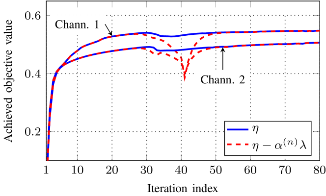
Fig. 1: Convergence of Algorithm 1 with $\bar{P}=40$dBm and $\bar{C}_{b}=50$ Mnats/s.

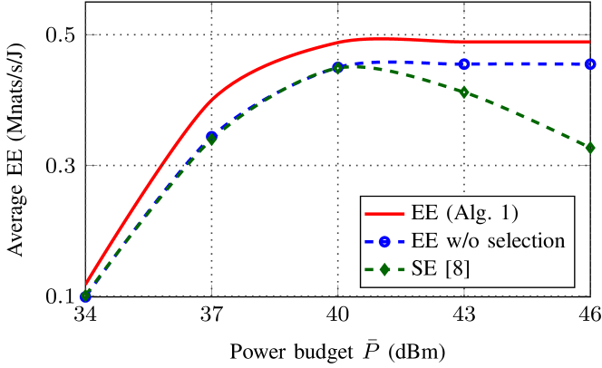
Fig. 2: Average EE versus the per-RU transmit power budget $\bar{P}$ with $\bar{C}_{b}=50$ Mnats/s.

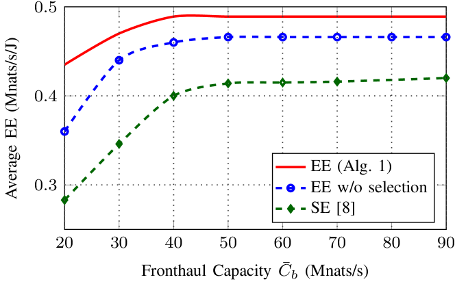
Fig. 3: Average EE versus the fronthaul capacity $\bar{C}_{b}$ with $\bar{P}=43$ dBm.

Fig. 2 compares the achieved EE versus the different transmit power budgets for two strategies, i.e., maxSE in [8] and maxEE (Algorithm 1), both using multivariate compression. We additionally illustrate the performance of EEmax without using RU-user selection scheme to highlight the impact of the selection strategy. Note that the numerical results on SEmax and EEmax comparison presented in [21],[22] imply that the EEmax (without selection) is in fact the SEmax in the low-power regime, while in the high-power regime the SEmax reduces and the EEmax remains unchanged. As can be seen, the performance shown in Fig. 2 is consistent with those observations made previously. On the other hand, Algorithm 1 which adopts the RU-user selection scheme outperforms the others for both low and high power regions. This is easily understood since the selection mechanism will switch off RU-user transmission links that do not offer a significant improvement in achieved SE, saving power consumption remarkably.

Achieved EE versus the fronthaul capacity $\bar{C}_{b}$ is shown in Fig. 3. We can see that the achieved EE values for three schemes increase following the increase of $\bar{C}_{b}$ due to the fact that all BSs are allowed to transmit at higher data rates. However, the EEs achieved by the EEmax strategies saturate after a certain value of $\bar{C}_{b}$ (e.g., $\bar{C}_{b}=$40 Mnats/s for Algorithm 1), while SEmax scheme keeps improving as $\bar{C}_{b}$ increases. In fact, SEmax scheme always uses all available power to obtain more gain in achievable throughput. EEmax schemes, on the other hand, aim at finding the optimal trade-off between achieved sum rate and the total power consumption of the network.

V Conclusion

We have considered a C-RAN downlink transmission where multivariate compression fronthaul is adopted to generate the BB signals, which are conveyed to RUs through limited capacity fronthaul links. We have studied the joint design of precoding, multivariate compression and RU-user selection that maximizes the EE measure. The optimization problem is in fact a rank-constrained mixed Boolean nonconvex program. We have applied relaxation techniques to drop the rank constraint and convert the problem in a continuous domain. We have also used DC programming to derive a low-complex iterative method to solve the considered nonconvex continuous problem. The goal is to compute a stationary point fulfilling the KKT optimality conditions. The effectiveness of proposed algorithm has been demonstrated by the numerical results.

Appendix

We prove the first claim by leveraging the result in [12]. For the ease of description, we pose problem (20) at iteration $n+1$ in a general form as

$${\textstyle\max_{{\bf s}\in{\cal S}^{(n)}({\bf s})}}\ \ f_{0}({\bf s})\ \ \text{s.t.}\ \{p({\bf s})\geq 0\}$$ (21)

where $f_{0}({\bf s})\triangleq\eta-\alpha^{(n)}\lambda$, $p({\bf s})\triangleq\lambda+\Phi(\bm{\phi},\bm{\phi}^{(n)})$ and ${\cal S}^{(n)}({\bf{\bf s}})$ is the feasible set, i.e., ${\cal S}^{(n)}({\bf s})\triangleq\{{\bf s}\ |\ \eqref{eq:power},\eqref{eq:min:connectivity},\eqref{eq:PSD},\eqref{eq:rate:epi},$ $\eqref{eq:power:consumption:epi},\eqref{eq:infererence:epi},\eqref{eq:pow:precoderi:approx},\eqref{eq:EE:epi:approx},\eqref{eq:SINR:epi:approx},\eqref{eq:BH:approx}\}$. We also denote $I_{{\cal S}^{(n)}}({\bf s})$ and $\partial I_{{\cal S}^{(n)}}({\bf s})$ as the indicator function and the normal cone of ${\cal S}^{(n)}({\bf s})$ [23]. Recall the KKT conditions for solution of $\lambda$ at iteration $n+1$ which is given by

$$-\alpha^{(n)}+\mu^{(n+1)}+\vartheta^{(n+1)}=0;\ \lambda\vartheta^{(n+1)}=0;\ \lambda\geq 0$$ (22)

where $\mu^{(n+1)}$and $\vartheta^{(n+1)}$ are the Lagrangian multipliers corresponding to $p({\bf s})\geq 0$ and $\lambda\geq 0$, respectively. Let us assume $\underset{n\rightarrow+\infty}{\lim}\|\bm{\phi}^{(n+1)}-\bm{\phi}^{(n)}\|_{2}\neq 0$. One immediately has $\alpha^{(n)}\rightarrow+\infty$ and $\lambda>0$. The latter is due to the fact that whenever $\lambda=0$, then $\phi_{b,k}\in\{0,1\},\forall b,k$ and $\|\bm{\phi}^{(n+1)}-\bm{\phi}^{(n)}\|_{2}=0$ (i.e., $\phi_{b,k}$ is fixed). Since $\lambda>0$ means $\vartheta^{(n+1)}=0$ by (22), then $\mu^{(n+1)}\rightarrow+\infty$. Next, we consider the KKT condition for the Lagrangian function of (21) given by

$$\nabla_{{\bf s}}f_{0}({\bf s}^{(n+1)})+\mu^{(n+1)}\nabla_{{\bf s}}p({\bf s}^{(n+1)})+\partial I_{{\cal S}^{(n)}}({\bf s}^{(n+1)})\in 0$$ (23)

If dividing (23) by $\mu^{(n+1)}$ and let $n\rightarrow+\infty$, one has $\nabla_{{\bf s}}p(\tilde{{\bf s}})+\partial I_{{\cal S}^{(n)}}(\tilde{{\bf s}})\in 0$ which violates the Mangasarian–Fromovitz constraint qualification, i.e., $\nabla_{{\bf s}}p(\tilde{{\bf s}})$ and $\partial I_{{\cal S}^{(n)}}(\tilde{{\bf s}})$ are not positive-linearly independent at $\tilde{{\bf s}}$. This implies the contradiction with assumption of $\alpha^{(n+1)}\rightarrow+\infty$, and thus existing a finite integer $n_{0}$ such that $\alpha^{(n)}=\alpha^{(n_{0})}$ for $n\geq n_{0}$. Thereby we obtain $\|\bm{\phi}^{(n+1)}-\bm{\phi}^{(n)}\|_{2}=0$ leading to $\lambda=0$. Thus, $\underset{n\rightarrow+\infty}{\lim}\lambda^{(n)}=0$ which shows the first claim.

Next, we show that the limit point of Algorithm 1 fulfills the KKT conditions. By the above arguments, $\phi_{b,k}^{(n)},\forall b,k$ converges into a Boolean set $\{0,1\}$ at iteration $n\geq n_{0}$. At this point, follow exactly the convergence proof in [10] and remark that the feasible set of problem is bounded above by the power constraint, we have the stationary point of Algorithm 1 guaranteeing the KKT optimality conditions of (20). This completes the proof.

References

- [1] Qualcomm, “The 1000x data challenge,” tech. rep. [Online]. Available: http://www.qualcomm.com/1000x.
- [2] Ericsson White Paper, “More than 50 billion connected devices.” Ericsson, Tech. Rep. 284 23-3149 Uen, Feb 2011.
- [3] D. Gesbert, S. Hanly, H. Huang, S. S. Shitz, O. Simeone, and W. Yu, “Multi-cell MIMO cooperative networks: A new look at interference,” IEEE J. Sel. Areas Commun., vol. 28, no. 9, pp. 1380–1408, Dec. 2010.
- [4] C. Yang, S. Han, X. Hou, and A. F. Molisch, “How do we design CoMP to achieve its promised potential?” IEEE Wireless Commun., vol. 20, no. 1, pp. 67–74, February 2013.
- [5] J. Wu, “Green wireless communications: from concept to reality [industry perspectives],” IEEE Wireless Commun., vol. 19, no. 4, pp. 4–5, August 2012.
- [6] C. Mobile, “C-ran: the road towards green ran,” White Paper, vol. 2, 2011.
- [7] M. Peng, C. Wang, V. Lau, and H. V. Poor, “Fronthaul-constrained cloud radio access networks: insights and challenges,” IEEE Wireless Commun., vol. 22, no. 2, pp. 152–160, April 2015.
- [8] S. H. Park, O. Simeone, O. Sahin, and S. Shamai, “Joint precoding and multivariate backhaul compression for the downlink of cloud radio access networks,” IEEE Trans. Signal Process., vol. 61, no. 22, pp. 5646–5658, Nov 2013.
- [9] S. H. Park, O. Simeone, O. Sahin, and S. S. Shitz, “Fronthaul compression for cloud radio access networks: Signal processing advances inspired by network information theory,” IEEE Signal Process. Mag., vol. 31, no. 6, pp. 69–79, Nov 2014.
- [10] B. R. Marks and G. P. Wright, “A general inner approximation algorithm for nonconvex mathematical programs,” Operations Research, vol. 26, no. 4, pp. 681–683, Jul.-Aug. 1978.
- [11] A. Beck, A. Ben-Tal, and L. Tetruashvili, “A sequential parametric convex approximation method with applications to nonconvex truss topology design problem,” J. Global Optim., vol. 47, no. 1, pp. 29–51, 2010.
- [12] H. A. Le Thi, T. P. Dinh et al., “DC programming and DCA for general DC programs,” in Advanced Computational Methods for Knowledge Engineering. Springer, 2014, pp. 15–35.
- [13] A. El Gamal and Y.-H. Kim, Network information theory. Cambridge university press, 2011.
- [14] S. Boyd and L. Vandenberghe, Convex optimization. Cambridge university press, 2004.
- [15] D. Nguyen, L. N. Tran, P. Pirinen, and M. Latva-aho, “On the spectral efficiency of full-duplex small cell wireless systems,” IEEE Trans. Wireless Commun., vol. 13, no. 9, pp. 4896–4910, Sept 2014.
- [16] A. Ben-Tal and A. Nemirovski, Lectures on modern convex optimization. Philadelphia: MPS-SIAM Series on Optimization, SIAM, 2001.
- [17] Q. D. Vu, L. N. Tran, R. Farrell, and E. K. Hong, “Energy-efficient zero-forcing precoding design for small-cell networks,” IEEE Trans. Commun., vol. 64, no. 2, pp. 790–804, Feb 2016.
- [18] A. Ben-Tal and A. Nemirovski, “On the polyhedral approximations of the second-order cone,” Mathematics of Operations Research, vol. 26, no. 2, pp. 193–205, May 2001.
- [19] K.-G. Nguyen, L.-N. Tran, O. Tervo, Q.-D. Vu, and M. Juntti, “Achieving energy efficiency fairness in multicell multiuser MISO downlink,” IEEE Commun. Lett., vol. 19, no. 8, pp. 1426 – 1429, Aug. 2015.
- [20] Y. Cheng, M. Pesavento, and A. Philipp, “Joint network optimization and downlink beamforming for CoMP transmissions using mixed integer conic programming,” IEEE Trans. Signal Process., vol. 61, no. 16, pp. 3972–3987, Aug 2013.
- [21] D. Nguyen, L.-N. Tran, P. Pirinen, and M. Latva-aho, “Precoding for full duplex multiuser MIMO systems: Spectral and energy efficiency maximization,” IEEE Trans. Signal Process., vol. 61, no. 16, pp. 4038–3050, Aug. 2013.
- [22] D. W. K. Ng, E. S. Lo, and R. Schober, “Energy-efficient resource allocation in multi-cell OFDMA systems with limited backhaul capacity,” IEEE Trans. Wireless Commun., vol. 11, no. 10, pp. 3618–3631, Oct. 2012.
- [23] R. T. Rockafellar, Convex analysis. Princeton university press, 2015.