Two classes of nonlocal Evolution Equations related by a shared Traveling Wave Problem

Abstract

We consider reaction-diffusion equations and Korteweg-de Vries-Burgers (KdVB) equations, i.e. scalar conservation laws with diffusive-dispersive regularization. We review the existence of traveling wave solutions for these two classes of evolution equations. For classical equations the traveling wave problem (TWP) for a local KdVB equation can be identified with the TWP for a reaction-diffusion equation. In this article we study this relationship for these two classes of evolution equations with nonlocal diffusion/dispersion. This connection is especially useful, if the TW equation is not studied directly, but the existence of a TWS is proven using one of the evolution equations instead. Finally, we present three models from fluid dynamics and discuss the TWP via its link to associated reaction-diffusion equations.

1 Introduction

We will consider two classes of (nonlocal) evolution equations and study the associated traveling wave problems in parallel: On the one hand, we consider scalar conservation laws with (nonlocal) diffusive-dispersive regularization

$$\partial_{t}{u}+\partial_{x}{}f(u)=\epsilon\mathcal{L}_{1}[u]+\delta\partial_{x}{}\mathcal{L}_{2}[u]\ ,\quad t>0\ ,\quad x\in\mathbb{R}\ ,$$ (1)

for some nonlinear function $f:\mathbb{R}\to\mathbb{R}$, Lévy operators $\mathcal{L}_{1}$ and $\mathcal{L}_{2}$, as well as constants $\epsilon,\delta\in\mathbb{R}$. The Fourier multiplier operators $\mathcal{L}_{1}$ and $\partial_{x}{}\mathcal{L}_{2}$ model diffusion and dispersion, respectively. On the other hand, we consider scalar reaction-diffusion equations

$$\partial_{t}{u}=r(u)+\sigma\mathcal{L}_{3}[u]\ ,\quad t>0\ ,\quad x\in\mathbb{R}\ ,$$ (2)

for some positive constant $\sigma$, as well as a nonlinear function $r:\mathbb{R}\to\mathbb{R}$ and a Lévy operator $\mathcal{L}_{3}$ modeling reaction and diffusion, respectively.

Definition 1.

A traveling wave solution (TWS) of an evolution equation–such as (1) and (2)–is a solution $u(x,t)=\bar{u}(\xi)$ whose profile $\bar{u}$ depends on $\xi:=x-ct$ for some wave speed $c$. Moreover, the profile $\bar{u}\in C^{2}(\mathbb{R})$ is assumed to approach distinct endstates $u_{\pm}$ such that

$$\lim_{\xi\to\pm\infty}\bar{u}(\xi)=u_{\pm}\ ,\qquad\lim_{\xi\to\pm\infty}\bar{u}^{(n)}(\xi)=0\quad\text{with $n=1,2$.}$$ (3)

Such a TWS is also known as a front in the literature. A TWS $(\bar{u},c)$ is called monotone, if its profile $\bar{u}$ is a monotone function.

Definition 2.

The traveling wave problem (TWP) associated to an evolution equation is to study for some distinct endstates $u_{\pm}$ the existence of a TWS $(\bar{u},c)$ in the sense of Definition 1.

We want to identify classes of evolutions equations of type (1) and (2), which lead to the same TWP. This connection is especially useful, if the TWP is not studied directly, but the existence of a TWS is proven using one of the evolution equations instead. A classical example of (1) is a scalar conservation law with local diffusive-dispersive regularization

$$\partial_{t}{u}+\partial_{x}{}f(u)=\epsilon\partial^{2}_{x}{u}+\delta\partial^{3}_{x}{u}\ ,\quad t>0\ ,\quad x\in\mathbb{R}\ ,$$ (4)

for some nonlinear function $f:\mathbb{R}\to\mathbb{R}$ and some constants $\epsilon>0$ and $\delta\in\mathbb{R}$. Equation (4) with Burgers flux $f(u)=u^{2}$ is known as Korteweg-de Vries-Burgers (KdVB) equation; hence we refer to Equation (4) with general $f$ as generalized KdVB equation and Equation (1) as nonlocal generalized KdVB equation. A TWS $(\bar{u},c)$ satisfies the traveling wave equation (TWE)

$$-c\bar{u}^{\prime}+f^{\prime}(\bar{u})\ \bar{u}^{\prime}=\epsilon\bar{u}^{\prime\prime}+\delta\bar{u}^{\prime\prime\prime}\ ,\quad\xi\in\mathbb{R}\ ,$$ (5)

or integrating on $(-\infty,\xi]$ and using (3),

$$h(\bar{u}):=f(\bar{u})-c\bar{u}-(f(u_{-})-c\ u_{-})=\epsilon\bar{u}^{\prime}+\delta\bar{u}^{\prime\prime}\ ,\quad\xi\in\mathbb{R}\ .$$ (6)

However, the TW ansatz $v(x,t)=\bar{u}(x-\epsilon t)$ for the scalar reaction-diffusion equation

$$\partial_{t}{v}=-h(v)+\delta\partial^{2}_{x}{v}\ ,\quad t>0\ ,\quad x\in\mathbb{R}\ ,$$ (7)

leads to the same TWE (6) except for a different interpretation of the parameters. The traveling wave speeds in the TWP of (4) and (7) are $c$ and $\epsilon$, respectively. For fixed parameters $c$, $\epsilon$, and $\delta$, the existence of a traveling wave profile $\bar{u}$ satisfying (3) and (6) reduces to the existence of a heteroclinic orbit for this ODE. This is an example, where the existence of TWS is studied directly via the TWE.

A first example, where the TWE is not studied directly, is the TWP for a nonlocal KdVB equation (1) with $\mathcal{L}_{1}[u]=\partial^{2}_{x}{u}$ and $\mathcal{L}_{2}[u]=\phi_{\epsilon}\ast u-u$ for some even non-negative function $\phi\in L^{1}(\mathbb{R})$ with compact support and unit mass, where $\phi_{\epsilon}(\cdot):=\phi(\cdot/\epsilon)/\epsilon$ with $\epsilon>0$. It has been derived as a model for phase transitions with long range interactions close to the surface, which supports planar TWS associated to undercompressive shocks of (51), see [41]. In particular, the TWP for a cubic flux function $f(u)=u^{3}$ is related to the TWP for a reaction-diffusion equation (2) with $\mathcal{L}_{3}[u]=\mathcal{L}_{2}[u]$. The existence of TWS for this reaction-diffusion equation has been proven via a homotopy of (2) to a classical reaction-diffusion model (7), see [11].

Outline. In Section 2 we collect background material on Lévy operators $\mathcal{L}$, which will model diffusion in our nonlocal evolution equations. Special emphasize is given to convolution operators and Riesz-Feller operators. In Section 3 we review the classical results on the TWP for reaction-diffusion equations (7) and generalized Korteweg-de Vries-Burgers equation (4). We study their relationship in detail, especially the classification of function $h(u)$, which will be used again in Section 4. In Section 4, first we review the results on TWP for nonlocal reaction-diffusion equations (2) with operators $\mathcal{L}_{3}$ of convolution type and Riesz-Feller type, respectively. Finally, we study the example of nonlocal generalized Korteweg-de Vries-Burgers equation modeling a shallow water flow [33] and Fowler’s equation modeling dune formation [26],

$$\partial_{t}{u}+\partial_{x}{}u^{2}=\partial^{2}_{x}{}u-\partial_{x}{}\mathcal{D}^{1/3}_{+}u\ ,\quad t>0\ ,\quad x\in\mathbb{R}\ ,$$ (8)

where $\mathcal{D}^{\alpha}_{+}$ is a Caputo derivative. In the Appendix, we collect background material on Caputo derivatives $\mathcal{D}^{\alpha}_{+}$ and the shock wave theory for scalar conservation laws, which will explain the importance of the TWP for KdVB equations.

Notations. We use the conventions in probability theory, and define the Fourier transform $\mathcal{F}$ and its inverse $\mathcal{F}^{-1}$ for $g\in L^{1}(\mathbb{R})$ and $x,k\in\mathbb{R}$ as

$$\mathcal{F}[g](k):=\int_{\mathbb{R}}\;{\operatorname{e}^{+\operatorname{i}kx}g(x)}\;\,\operatorname{d}\!x\,\ ;\qquad\mathcal{F}^{-1}[g](x):=\tfrac{1}{2\pi}\int_{\mathbb{R}}\;{\operatorname{e}^{-\operatorname{i}kx}g(k)}\;\,\operatorname{d}\!k\,\ .$$

In the following, $\mathcal{F}$ and $\mathcal{F}^{-1}$ will denote also their respective extensions to $L^{2}(\mathbb{R})$.

2 Lévy Operators

A Lévy process is a stochastic process with independent and stationary increments which is continuous in probability [9, 30, 42]. Therefore a Lévy process is characterized by its transition probabilities $p(t,x)$, which evolve according to an evolution equation

$$\partial_{t}{p}=\mathcal{L}p$$ (9)

for some operator $\mathcal{L}$, also called a Lévy operator. First, we define Lévy operators on the function spaces $C_{0}(\mathbb{R}):=\{f\in C(\mathbb{R})\,|\,\lim_{|x|\to\infty}f(x)=0\}$ and $C^{2}_{0}(\mathbb{R}):=\{f,f^{\prime},f^{\prime\prime}\in C_{0}(\mathbb{R})\}$.

Definition 3.

The family of Lévy operators in one spatial dimension consists of operators $\mathcal{L}$ defined for $f\in C^{2}_{0}(\mathbb{R})$ as

$$\mathcal{L}f(x)=\tfrac{1}{2}Af^{\prime\prime}(x)+\gamma\ f^{\prime}(x)+\int_{\mathbb{R}}\;{\big{(}f(x+y)-f(x)-y\ f^{\prime}(x)1_{(-1,1)}(y)\big{)}}\;{\nu(\,\operatorname{d}\!y)}\,$$ (10)

for some constants $A\geq 0$ and $\gamma\in\mathbb{R}$, and a measure $\nu$ on $\mathbb{R}$ satisfying

$$\nu(\{0\})=0\quad\text{and}\quad\int_{\mathbb{R}}\;{\min(1,|y|^{2})}\;{\nu(\,\operatorname{d}\!y)}\,<\infty\,.$$

Remark 1.

The function $f(x+y)-f(x)-y\ f^{\prime}(x)1_{(-1,1)}(y)$ is integrable with respect to $\nu$, because it is bounded outside of any neighborhood of $0$ and

$$f(x+y)-f(x)-y\ f^{\prime}(x)1_{(-1,1)}(y)=O(|y|^{2})\quad\text{as}\quad|y|\to 0$$

for fixed $x$. The indicator function $c(y)=1_{(-1,1)}(y)$ is only one possible choice to obtain an integrable integrand. More generally, let $c(y)$ be a bounded measurable function from $\mathbb{R}$ to $\mathbb{R}$ satisfying $c(y)=1+o(|y|)$ as $|y|\to 0$, and $c(y)=O(1/|y|)$ as $|y|\to\infty$. Then (10) is rewritten as

$$\mathcal{L}f(x)=\tfrac{1}{2}Af^{\prime\prime}(x)+\gamma_{c}\ f^{\prime}(x)+\int_{\mathbb{R}}\;{\big{(}f(x+y)-f(x)-y\ f^{\prime}(x)c(y)\big{)}}\;{\nu(\,\operatorname{d}\!y)}\,\ ,$$ (11)

with $\gamma_{c}=\gamma+\int_{\mathbb{R}}\;{y\ (c(y)-1_{(-1,1)}(y))}\;{\nu(\,\operatorname{d}\!y)}\,$.

Alternative choices for $c$:

1. If a Lévy measure $\nu$ satisfies $\int_{|y|<1}\;{|y|}\;{\nu(\,\operatorname{d}\!y)}\,<\infty$ then $c\equiv 0$ is admissible.

2. If a Lévy measure $\nu$ satisfies $\int_{|y|>1}\;{|y|}\;{\nu(\,\operatorname{d}\!y)}\,<\infty$ then $c\equiv 1$ is admissible.

We note that $A$ and $\nu$ are invariant no matter what function $c$ we choose.

Examples.

1. The Lévy operators

   $$\mathcal{L}f=\int_{\mathbb{R}}\;{\big{(}f(x+y)-f(x)\big{)}}\;{\nu(\,\operatorname{d}\!y)}\,$$ (12)

   are infinitesimal generators associated to a compound Poisson process with finite Lévy measure $\nu$ satisfying (c 0). The special case of $\nu(\,\operatorname{d}\!y)=\phi(-y)\,\operatorname{d}\!y$ for some function $\phi\in L^{1}(\mathbb{R})$ yields

   $$\mathcal{L}f(x)=\int_{\mathbb{R}}\;{\big{(}f(x+y)-f(x)\big{)}}\;{\phi(-y)\,\operatorname{d}\!y}\,=\big{(}\phi\ast f-\int_{\mathbb{R}}\;{\phi}\;\,\operatorname{d}\!y\,\ f\big{)}(x)\ .$$ (13)

2. Riesz-Feller operators. The Riesz-Feller operators of order $a$ and asymmetry $\theta$ are defined as Fourier multiplier operators

   $$\mathcal{F}[D^{a}_{\theta}f](k)=\psi^{a}_{\theta}(k)\ \mathcal{F}[f](k)\ ,\qquad k\in\mathbb{R}\ ,$$ (14)

   with symbol $\psi^{a}_{\theta}(k)=-|k|^{a}\exp\left[\operatorname{i}\ \operatorname{sgn}(k)\ \theta\pi/2\right]$ such that $(a,\theta)\in\mathfrak{D}_{a,\theta}$ and

   $$\mathfrak{D}_{a,\theta}:=\{\,{(a,\theta)\in\mathbb{R}^{2}}\,|\,{0<a\leq 2\ ,\quad|\theta|\leq\min\{a,2-a\}}\,\}\ .$$

   

   Figure 1: The family of Fourier multipliers $\psi^{a}_{\theta}(k)=-|k|^{a}\exp\big{[}\operatorname{i}\operatorname{sgn}(k)\theta\pi/2)\big{]}$ has two parameters $a$ and $\theta$. Some Fourier multiplier operators $\mathcal{F}[Tf](k)=\psi^{a}_{\theta}(k)\ \mathcal{F}[f](k)$ are inserted in the parameter space $(a,\theta)$: partial derivatives and Caputo derivatives $\mathcal{D}^{\alpha}_{+}$ with $0<\alpha<1$. The Riesz-Feller operators $D^{a}_{\theta}$ are those operators with parameters $(a,\theta)\in\mathfrak{D}_{a,\theta}$. The set $\mathfrak{D}_{a,\theta}$ is also called Feller-Takayasu diamond and depicted as a shaded region, see also [36].

   Special cases of Riesz-Feller operators are

   • Fractional Laplacians $-(-\Delta)^{a/2}$ on $\mathbb{R}$ with Fourier symbol $-|k|^{a}$ for $0<a\leq 2$. In particular, fractional Laplacians are the only symmetric Riesz-Feller operators with $-(-\Delta)^{a/2}=D^{a}_{0}$ and $\theta\equiv 0$.

   • Caputo derivatives $-\mathcal{D}^{\alpha}_{+}$ with $0<\alpha<1$ are Riesz-Feller operators with $a=\alpha$ and $\theta=-\alpha$, such that $-\mathcal{D}^{\alpha}_{+}=D^{\alpha}_{-\alpha}$, see also Section A.

   • Derivatives of Caputo derivatives $\partial_{x}{}\mathcal{D}^{\alpha}_{+}$ with $0<\alpha<1$ are Riesz-Feller operators with $a=1+\alpha$ and $\theta=1-\alpha$, such that $\partial_{x}{}\mathcal{D}^{\alpha}_{+}=D^{1+\alpha}_{1-\alpha}$.

Next we consider the Cauchy problem

$$\partial_{t}{u}(x,t)=D^{a}_{\theta}{}[u(\cdot,t)](x)\ ,\quad u(x,0)=u_{0}(x)\ ,$$ (15)

for $(x,t)\in\mathbb{R}\times(0,\infty)$ and initial datum $u_{0}$.

Proposition 1.

For $(a,\theta)\in\mathfrak{D}_{a,\theta}$ and $1\leq p<\infty$, the Riesz-Feller operator $D^{a}_{\theta}$ generates a strongly continuous $L^{p}$-semigroup

$$S_{t}:L^{p}(\mathbb{R})\to L^{p}(\mathbb{R})\ ,\quad u_{0}\mapsto S_{t}u_{0}=G^{a}_{\theta}(\cdot,t)\ast u_{0}\ ,$$

with heat kernel $G^{a}_{\theta}(x,t)=\mathcal{F}^{-1}[\exp(t\ \psi^{a}_{\theta}(\cdot))](x)$. In particular, $G^{a}_{\theta}(x,t)$ is the probability measure of a Lévy strictly $a$-stable distribution.

For $(a,\theta)\in\{(1,1),(1,-1)\}$, the probability measure $G^{a}_{\theta}$ is a delta distribution, e.g. $G^{1}_{1}(x,t)=\delta_{x+t}$ and $G^{1}_{-1}(x,t)=\delta_{x-t}$, and is called trivial [42, Definition 13.6]. However, we are interested in non-trivial probability measures $G^{a}_{\theta}$ for

$$(a,\theta)\in\mathfrak{D}_{a,\theta}^{\diamond}:=\{\,{(a,\theta)\in\mathfrak{D}_{a,\theta}}\,|\,{|\theta|<1}\,\}\ ,$$

such that $\mathfrak{D}_{a,\theta}=\mathfrak{D}_{a,\theta}^{\diamond}\cup\{(1,1),\ (1,-1)\}$. Note, nonlocal Riesz-Feller $D^{a}_{\theta}$ operators are those with parameters

$$(a,\theta)\in\mathfrak{D}_{a,\theta}^{\bullet}:=\{\,{(a,\theta)\in\mathfrak{D}_{a,\theta}}\,|\,{0<a<2\ ,\quad|\theta|<1}\,\},$$

such that $\mathfrak{D}_{a,\theta}^{\diamond}=\mathfrak{D}_{a,\theta}^{\bullet}\cup\{(2,0)\}$.

Proposition 2 ([6, Lemma 2.1]).

For $(a,\theta)\in\mathfrak{D}_{a,\theta}^{\diamond}$ the probability measure $G^{a}_{\theta}$ is absolutely continuous with respect to the Lebesgue measure and possesses a probability density which will be denoted again by $G^{a}_{\theta}$. For all $(x,t)\in\mathbb{R}\times(0,\infty)$ the following properties hold;

1. $G^{a}_{\theta}(x,t)\geq 0$. If $\theta\neq\pm a$ then $G^{a}_{\theta}(x,t)>0$;

2. $\|G^{a}_{\theta}(\cdot,t)\|_{L^{1}(\mathbb{R})}=1$;

3. $G^{a}_{\theta}(x,t)=t^{-1/a}G^{a}_{\theta}(xt^{-1/a},1)$;

4. $G^{a}_{\theta}(\cdot,s)\ast G^{a}_{\theta}(\cdot,t)=G^{a}_{\theta}(\cdot,s+t)$ for all $s,t\in(0,\infty)$;

5. $G^{a}_{\theta}\in C^{\infty}_{0}(\mathbb{R}\times(0,\infty))$.

The Lévy measure $\nu$ of a Riesz-Feller operator $D^{a}_{\theta}$ with $(a,\theta)\in\mathfrak{D}_{a,\theta}^{\bullet}$ is absolutely continuous with respect to Lebesgue measure and satisfies

$$\nu(\,\operatorname{d}\!y)=\begin{cases}c_{-}(\theta)y^{-1-a}\ \,\operatorname{d}\!y&\text{on }(0,\infty)\ ,\\ c_{+}(\theta)|y|^{-1-a}\ \,\operatorname{d}\!y&\text{on }(-\infty,0)\ ,\end{cases}$$ (16)

with $c_{\pm}(\theta)=\Gamma(1+a)\sin((a\pm\theta)\pi/2)/\pi$, see [36, 43].

To study a TWP for evolution equations involving Riesz-Feller operators, it is necessary to extend the Riesz-Feller operators to $C^{2}_{b}(\mathbb{R})$. Their singular integral representations (10) may be used to accomplish this task.

Theorem 1 ([6]).

If $(a,\theta)\in\mathfrak{D}_{a,\theta}^{\bullet}$ with $a\neq 1$, then for all $f\in\mathcal{S}(\mathbb{R})$ and $x\in\mathbb{R}$

$$D^{a}_{\theta}f(x)= \frac{c_{+}(\theta)-c_{-}(\theta)}{1-a}f^{\prime}(x)$$

$$+c_{+}(\theta)\int_{0}^{\infty}\;{\frac{f(x+y)-f(x)-f^{\prime}(x)\,y1_{(-1,1)}(y)}{y^{1+a}}}\;\,\operatorname{d}\!y\,$$ (17)

$$+c_{-}(\theta)\int_{0}^{\infty}\;{\frac{f(x-y)-f(x)+f^{\prime}(x)\,y1_{(-1,1)}(y)}{y^{1+a}}}\;\,\operatorname{d}\!y\,$$

with $c_{\pm}(\theta)=\Gamma(1+a)\sin((a\pm\theta)\pi/2)/\pi$. Alternative representations are

• If $0<a<1$, then

  $$D^{a}_{\theta}f(x)=c_{+}(\theta)\int_{0}^{\infty}\;{\frac{f(x+y)-f(x)}{y^{1+a}}}\;\,\operatorname{d}\!y\,+c_{-}(\theta)\int_{0}^{\infty}\;{\frac{f(x-y)-f(x)}{y^{1+a}}}\;\,\operatorname{d}\!y\,\,.$$

• If $1<a<2$, then

  $$D^{a}_{\theta}f(x)=c_{+}(\theta)\int_{0}^{\infty}\;{\frac{f(x+y)-f(x)-f^{\prime}(x)\,y}{y^{1+a}}}\;\,\operatorname{d}\!y\,\\ +c_{-}(\theta)\int_{0}^{\infty}\;{\frac{f(x-y)-f(x)+f^{\prime}(x)\,y}{y^{1+a}}}\;\,\operatorname{d}\!y\,\,.$$ (18)

These representations allow to extend Riesz-Feller operators $D^{a}_{\theta}$ to $C^{2}_{b}(\mathbb{R})$ such that $D^{a}_{\theta}C^{2}_{b}(\mathbb{R})\subset C_{b}(\mathbb{R})$. For example, one can show

Proposition 3 ([6, Proposition 2.4]).

For $(a,\theta)\in\mathfrak{D}_{a,\theta}$ with $1<a<2$, the integral representation (18) of $D^{a}_{\theta}$ is well-defined for functions $f\in C^{2}_{b}(\mathbb{R})$ with

$$\sup_{x\in\mathbb{R}}|D^{a}_{\theta}f(x)|\leq\mathcal{K}\|{f^{\prime\prime}}\|_{C_{b}(\mathbb{R})}\frac{M^{2-a}}{2-a}+4\mathcal{K}\|f^{\prime}\|_{C_{b}(\mathbb{R})}\frac{M^{1-a}}{a-1}<\infty$$ (19)

for some positive constants $M$ and $\mathcal{K}=\frac{\Gamma(1+a)}{\pi}|\sin((a+\theta)\frac{\pi}{2})+\sin((a-\theta)\frac{\pi}{2})|$.

Estimate (19) is a key estimate, which is used to adapt Chen’s approach [19] to the TWP for nonlocal reaction-diffusion equations with Riesz-Feller operators [6].

3 TWP for classical evolution equations

In this section we review the importance of the TWP for reaction-diffusion equations and scalar conservation laws with higher-order regularizations, respectively.

3.1 reaction-diffusion equations

A scalar reaction-diffusion equations is a partial differential equation

$$\partial_{t}{u}=r(u)+\sigma\partial^{2}_{x}{u}\ ,\quad t>0\ ,\quad x\in\mathbb{R}\ ,$$ (20)

for some positive constant $\sigma>0$, as well as a nonlinear function $r:\mathbb{R}\to\mathbb{R}$ and second-order derivative $\partial^{2}_{x}{u}$ modeling reaction and diffusion, respectively. The TWP for given endstates $u_{\pm}$ is to study the existence of a TWS $(\bar{u},c)$ for (20) in the sense of Definition 1. If the profile $\bar{u}\in C^{2}(\mathbb{R})$ is bounded, then it satisfies $\lim_{\xi\to\pm\infty}\bar{u}^{(n)}(\xi)=0$ for $n=1,2$. A TWS $(\bar{u},c)$ satisfies the TWE

$$-c\bar{u}^{\prime}=r(\bar{u})+\sigma\bar{u}^{\prime\prime}\ ,\quad\xi\in\mathbb{R}\ .$$ (21)

phase plane analysis. A traveling wave profile $\bar{u}$ is a heteroclinic orbit of the TWE (21) connecting the endstates $u_{\pm}$. To identify necessary conditions on the existence of TWS, TWE (21) is written as a system of first-order ODEs for $u$, $v:=u^{\prime}$:

$$\frac{\,\operatorname{d}\!}{\,\operatorname{d}\!\xi}\binom{u}{v}=\binom{v}{(-r(u)-cv)/\sigma}=:F(u,v)\ ,\quad\xi\in\mathbb{R}\ .$$ (22)

First, an endstate $(u_{s},v_{s})$ of a heteroclinic orbit has to be a stationary state of $F$, i.e. $F(u_{s},v_{s})=0$, which implies $v_{s}\equiv 0$ and $r(u_{s})=0$. Second, $(u_{-},0)$ has to be an unstable stationary state of (22) and $(u_{+},0)$ either a saddle or a stable node of (22). As long as a stationary state $(u_{s},v_{s})$ is hyperbolic, i.e. the linearization of $F$ at $(u_{s},v_{s})$ has only eigenvalues $\lambda$ with non-zero real part, the stability of $(u_{s},v_{s})$ is determined by these eigenvalues. The linearization of $F$ at $(u_{s},v_{s})$ is

$$\operatorname{D}\!F(u_{s},v_{s})=\begin{pmatrix}0&1\\ -r^{\prime}(u_{s})/\sigma&-c/\sigma\end{pmatrix}\ .$$ (23)

Eigenvalues $\lambda_{\pm}$ of the Jacobian $\operatorname{D}\!F(u_{s},v_{s})$ satisfy the characteristic equation $\lambda^{2}+\lambda c/\sigma+r^{\prime}(u_{s})/\sigma=0$. Moreover, $\lambda_{-}+\lambda_{+}=-c/\sigma$ and $\lambda_{-}\lambda_{+}=r^{\prime}(u_{s})/\sigma$. The eigenvalues $\lambda_{\pm}$ of the Jacobian $\operatorname{D}\!F(u_{s},v_{s})$ are

$$\lambda_{\pm}=-\frac{c}{2\sigma}\pm\sqrt{\frac{c^{2}}{4\sigma^{2}}-\frac{r^{\prime}(u_{s})}{\sigma}}=\frac{-c\pm\sqrt{c^{2}-4\sigma r^{\prime}(u_{s})}}{2\sigma}\ .$$ (24)

Thus $r^{\prime}(u_{s})<0$ ensures that $(u_{s},0)$ is a saddle point, i.e. with one positive and one negative eigenvalue.

balance of potential. The potential $R$ (of the reaction term $r$) is defined as $R(u):=\int_{0}^{u}\;{r(\upsilon)}\;\,\operatorname{d}\!\upsilon\,$. The potentials of the endstates $u_{\pm}$ are called balanced if $R(u_{+})=R(u_{-})$ and unbalanced otherwise. A formal computation reveals a connection between the sign of $c$ and the balance of the potential $R(u)$: Multiplying TWE (21) with $\bar{u}^{\prime}$, integrating on $\mathbb{R}$ and using (3), yields

$$-c\|\bar{u}^{\prime}\|_{L^{2}}^{2}=\int_{u_{-}}^{u_{+}}\;{r(\upsilon)}\;\,\operatorname{d}\!\upsilon\,=R(u_{+})-R(u_{-})\ ,$$ (25)

since $\int_{\mathbb{R}}\;{\bar{u}^{\prime\prime}\bar{u}^{\prime}}\;\,\operatorname{d}\!\xi\,=0$ due to (3). Thus $-\operatorname{sgn}c=\operatorname{sgn}(R(u_{+})-R(u_{-}))$. In case of a balanced potential the wave speed $c$ is zero, hence the TWS is stationary.

Definition 4.

Assume $u_{-}>u_{+}$. A function $r\in C^{1}(\mathbb{R})$ with $r(u_{\pm})=0$ is

• monostable if $r^{\prime}(u_{-})<0$, $r^{\prime}(u_{+})>0$ and $r(u)>0$ for $u\in(u_{+},u_{-})$.

• bistable if $r^{\prime}(u_{\pm})<0$ and

  $$\exists u_{*}\in(u_{+},u_{-})\ :\ r(u)\begin{cases}<0&\text{for }u\in(u_{+},u_{*})\ ,\\ >0&\text{for }u\in(u_{*},u_{-})\ .\end{cases}$$

• unstable if $r^{\prime}(u_{\pm})>0$.

We chose a very narrow definition compared to [45]. Moreover, in most applications of reaction-diffusion equations a quantity $u$ models a density of a substance/population. In these situations only nonnegative states $u_{\pm}$ and functions $u$ are of interest.

Proposition 4 ([45, §2.2]).

Assume $\sigma>0$ and $u_{-}>u_{+}$.

• If $r$ is monostable, then there exists a positive constant $c_{*}$ such that for all $c\geq c_{*}$ there exists a monotone TWS $(\bar{u},c)$ of (20) in the sense of Definition 1. For $c<c_{*}$ no such monotone TWS exists (however oscillatory TWS may exist).

• If $r$ is bistable, then there exists an (up to translations) unique monotone TWS $(\bar{u},c)$ of (20) in the sense of Definition 1.

• If $r$ is unstable, then there does not exist a monotone TWS $(\bar{u},c)$ of (20).

If a TWS $(\bar{u},c)$ exists, then a closer inspection of the eigenvalues (24) at $(u_{+},0)$ indicates the geometry of the profile $\bar{u}$ for large $\xi$:

$$c^{2}-4\sigma r^{\prime}(u_{+})\begin{cases}\geq 0&\text{TWS with monotone decreasing profile~{}$\bar{u}$ for large $\xi$};\\ <0&\text{TWS with oscillating profile~{}$\bar{u}$ for large $\xi$}.\end{cases}$$

3.2 Korteweg-de Vries-Burgers equation (KdVB)

A generalized KdVB equation is a scalar partial differential equation

$$\partial_{t}{u}+\partial_{x}{}f(u)=\epsilon\partial^{2}_{x}{u}+\delta\partial^{3}_{x}{u},\quad x\in\mathbb{R},\quad t>0,$$ (26)

for some flux function $f:\mathbb{R}\to\mathbb{R}$ as well as constants $\epsilon>0$ and $\delta\in\mathbb{R}$. The TWP for given endstates $u_{\pm}$ is to study the existence of a TWS $(\bar{u},c)$ for (26) in the sense of Definition 1. The importance of the TWP for KdVB equations in the shock wave theory of (scalar) hyperbolic conservation laws is discussed in Section B. A TWS $(\bar{u},c)$ satisfies the TWE

$$-c\bar{u}^{\prime}+f^{\prime}(\bar{u})\ \bar{u}^{\prime}=\epsilon\bar{u}^{\prime\prime}+\delta\bar{u}^{\prime\prime\prime}\ ,\quad\xi\in\mathbb{R}\ ,$$ (27)

or integrating on $(-\infty,\xi]$ and using (3),

$$h(\bar{u}):=f(\bar{u})-c\bar{u}-(f(u_{-})-c\ u_{-})=\epsilon\bar{u}^{\prime}+\delta\bar{u}^{\prime\prime}\ ,\quad\xi\in\mathbb{R}\ .$$ (28)

connection with reaction-diffusion equation. A TWS $u(x,t)=\bar{u}(x-ct)$ of a generalized Korteweg-de Vries-Burgers equation (26) satisfies TWE (28). Thus $v(x,t)=\bar{u}(x-\epsilon t)$ is a TWS $(\bar{u},\epsilon)$ of the reaction-diffusion equation

$$\partial_{t}{v}=-h(v)+\delta\partial^{2}_{x}{v}\ ,\quad x\in\mathbb{R}\ ,\quad t>0\ .$$ (29)

phase plane analysis. Following the analysis of TWE (21) for a reaction-diffusion equation (20) with $r(u)=-h(u)$ and $\sigma=\delta$, necessary conditions on the parameters can be identified. First, a TWE is rewritten as a system of first-order ODEs with vector field $F$. Then the condition on stationary states implies that endstates $u_{\pm}$ and wave speed $c$ have to satisfy

$$f(u_{+})-f(u_{-})=c(u_{+}-u_{-})\ .$$ (30)

This condition is known in shock wave theory as Rankine-Hugoniot condition (54) on the shock triple $(u_{-},u_{+};c)$. The (nonlinear) stability of hyperbolic stationary states $(u_{s},v_{s})$ of $F$ is determined by the eigenvalues

$$\lambda_{\pm}=-\frac{1}{2}\frac{\epsilon}{\delta}\pm\frac{\sqrt{\epsilon^{2}+4\delta h^{\prime}(u_{s})}}{2|\delta|}$$ (31)

of the Jacobian $\operatorname{D}\!F(u_{s},v_{s})$. If $\epsilon,\delta>0$, then $(u_{+},0)$ is always either a saddle or stable node, and $h^{\prime}(u_{-})=f^{\prime}(u_{-})-c>0$ ensures that $(u_{-},0)$ is unstable. For example, Lax’ entropy condition (55), i.e. $f^{\prime}(u_{+})<c<f^{\prime}(u_{-})$, implies the latter condition.

convex flux functions.

Theorem 2.

Suppose $f\in C^{2}(\mathbb{R})$ is a strictly convex function. Let $\epsilon$, $\delta$ be positive and let $(u_{-},u_{+};c)$ satisfy the Rankine-Hugoniot condition (54) and the entropy condition (55), i.e. $u_{-}>u_{+}$. Then, there exists an (up to translations) unique TWS $(\bar{u},c)$ of (26) in the sense of Definition 1.

Proof.

We consider the associated reaction-diffusion equation (29), i.e. $\partial_{t}{u}=r(u)+\delta\partial^{2}_{x}{u}$ with $r(u)=-h(u)$. Due to (54) and (55), $r(u)$ is monostable in the sense of Definition 4. Moreover, function $r$ is strictly concave, since $r^{\prime\prime}(u)=-f^{\prime\prime}(u)$ and $f\in C^{2}(\mathbb{R})$ is strictly convex. In fact, $(u_{\pm},0)$ are the only stationary points of system (22), where $(u_{-},0)$ is a saddle point and $(u_{+},0)$ is a stable node. Thus, for all wave speeds $\epsilon$ there exists a TWS $(\bar{u},\epsilon)$ – with possibly oscillatory profile $\bar{u}$ – of reaction-diffusion equation (29). Moreover, $(\bar{u},c)$ is a TWS of (26), due to (27)–(29). ∎∎

The TWP for KdVB equations (26) with Burgers’ flux $f(u)=u^{2}$ has been investigated in [12]. The sign of $\delta$ in (26) is irrelevant, since it can be changed by a transformation $\tilde{x}=-x$ and $\tilde{u}(\tilde{x},t)=-u(x,t)$, see also [31]. First, the results in Theorem 2 on the existence of TWS and geometry of its profiles are proven. More importantly, the authors investigate the convergence of profiles $\bar{u}(\xi;\epsilon,\delta)$ in the limits $\epsilon\to 0$, $\delta\to 0$, as well as $\epsilon$ and $\delta$ tending to zero simultaneously. Assuming that the ratio $\delta/\epsilon^{2}$ remains bounded, they show that the TWS converge to the classical Lax shocks for this vanishing diffusive-dispersive regularization [12].

concave-convex flux functions.

Definition 5 ([34]).

A function $f\in C^{3}(\mathbb{R})$ is called concave-convex if

$$uf^{\prime\prime}(u)>0\quad\forall u\neq 0\ ,\quad f^{\prime\prime\prime}(0)\neq 0\ ,\quad\lim_{u\to\pm\infty}f^{\prime}(u)=+\infty\ .$$ (32)

Here the single inflection point is shifted without loss of generality to the origin. We consider a cubic flux function $f(u)=u^{3}$ as the prototypical concave-convex flux function with a single inflection point, see [29, 34].

Proposition 5 ([31, 28]).

Suppose $f(u)=u^{3}$ and $\epsilon>0$.

1. If $\delta\leq 0$ then a TWS $(\bar{u},c)$ of (26) exists if and only if $(u_{-},u_{+};c)$ satisfy the Rankine-Hugoniot condition (54) and the entropy condition (55).

2. If $\delta>0$ then a TWS $(\bar{u},c)$ of (26) exists for $u_{-}>0$ if and only if $u_{+}\in S(u_{-})$ with

   $$S(u_{-})=\begin{cases}[-\frac{u_{-}}{2},u_{-})&\,\text{ if }\,u_{-}\leq 2\beta\ ,\\ \{-u_{-}+\beta\}\cup[-\beta,u_{-})&\,\text{ if }\,u_{-}>2\beta\ ,\end{cases}$$ (33)

   where the coefficient $\beta$ is given by $\beta=\tfrac{\sqrt{2}}{3}\tfrac{\epsilon}{\sqrt{\delta}}$.

Proof.

Following the discussion from (26)–(29), we consider the associated reaction-diffusion equation (29), i.e. $\partial_{t}{u}=r(u)+\delta\partial^{2}_{x}{u}$ with $r(u)=-h(u)$. From this point of view, we need to classify the reaction term $r(u)=-h(u)$: Whereas $r(u_{-})=0$ by definition, $r(u_{+})=0$ if and only if $(u_{-},u_{+};c)$ satisfies the Rankine-Hugoniot condition (54). The Rankine-Hugoniot condition implies $c=u_{+}^{2}+u_{+}\ u_{-}+u_{-}^{2}$. Hence, the reaction term $r(u)$ has a factorization

$$r(u)=-(u^{3}-u_{-}^{3}-c(u-u_{-}))=-(u-u_{-})\ (u-u_{+})\ (u+u_{+}+u_{-})$$ (34)

Thus, $r(u)$ is a cubic polynomial with three roots $u_{1}\leq u_{2}\leq u_{3}$, such that $r(u)=-(u-u_{1})(u-u_{2})(u-u_{3})$. In case of distinct roots $u_{1}<u_{2}<u_{3}$ we deduce $r^{\prime}(u_{1})<0$, $r^{\prime}(u_{2})>0$ and $r^{\prime}(u_{3})<0$. The ordering of the roots $u_{\pm}$ and $u_{*}=-u_{-}-u_{+}$ depending on $u_{\pm}$ is visualized in Figure 2.

Figure 2: classification of the cubic reaction function $r(u)=-h(u)$ in (34) depending on its roots $u_{-}$, $u_{+}$ and $u_{*}=-u_{-}-u_{+}$ according to Definition 4.

Next, we will discuss the results in Proposition 5(b) (for $u_{-}>0$ and $\delta>0$) via results on the existence of TWS for a reaction-diffusion equation (29).

1. For $u_{+}<u_{*}<u_{-}$, function $r(u)$ is bistable, see also Figure 2. Due to Proposition 4, there exists an (up to translations) unique TWS $(\bar{u},\epsilon)$ with possibly negative wave speed. Under our assumption that the wave speed $\epsilon$ is positive, relation (25) yields the restriction $-u_{+}>u_{-}$. In fact, for $u_{-}>2\beta$ and $u_{+}=-u_{-}+\beta$ there exists a TWS $(\bar{u},\epsilon)$ for reaction-diffusion equation (29), see [31, Theorem 3.4]. The function $r$ is bistable with $u_{*}=-u_{-}-u_{+}=-\beta$, hence $f^{\prime}(u_{\pm})>c$. This violates Lax’ entropy condition (55) and is known in the shock wave theory as a slow undercompressive shock [34].

2. For $u_{*}<u_{+}<u_{-}$, function $r(u)$ is monostable, see Figure 2. Due to Proposition 4, there exists a critical wave speed $c_{*}$, such that monotone TWS $(\bar{u},\epsilon)$ for (29) exist for all $\epsilon\geq c_{*}$. However, not all endstates $(u_{-},u_{+})$ in the subset defined by $u_{*}<u_{+}<u_{-}$ admit a TWS $(\bar{u},c)$, see (33) and Figure 3b). The TWS $(\bar{u},c)$ associated to non-classical shocks appear again, with reversed roles for the roots $u_{+}$ and $u_{*}$: For $u_{-}>2\beta$ and $u_{+}=-\beta$, there exists a TWS $(\bar{u},\epsilon)$ for reaction-diffusion equation (29), see [31, Theorem 3.4]. These TWS form a horizontal halfline in Figure 3b) and divides the set defined by $u_{*}<u_{+}<u_{-}$ into two subsets. In particular, TWS exist only for endstates $(u_{-},u_{+})$ in the subset above this halfline.

3. For $u_{+}<u_{-}<u_{*}$, function $r(u)=-h(u)$ satisfies $r(u)<0$ for all $u\in(u_{+},u_{-})$, see also Figure 2. Thus the necessary condition (25) can not be fulfilled for positive $c=\epsilon$, hence there exists no TWS $(\bar{u},\epsilon)$ for the reaction-diffusion equation.

4. For $u_{*}<u_{-}<u_{+}$, function $r(u)$ is monostable with reversed roles of the endstates $u_{\pm}$, see Figure 2. Due to Proposition 4, there exists a TWS $(\bar{u},\epsilon)$ however satisfying $\lim_{\xi\to\mp\infty}\bar{u}(\xi)=u_{\pm}$.

If $\delta=0$, then equation (26) is a viscous conservation law, and its TWE (28) is a simple ODE $-\epsilon\bar{u}^{\prime}=r(\bar{u})$ with $r(u)=-h(u)$. Thus a heteroclinic orbit exists only for monostable $r(u)$, i.e. if the unstable node $u_{-}$ and the stable node $u_{+}$ are not separated by any other root of $r$.

If $\delta<0$, then we rewrite TWE (28) as $\epsilon\bar{u}^{\prime}=h(u)+|\delta|\bar{u}^{\prime\prime}$. It is associated to a reaction-diffusion equation $\partial_{t}{u}=h(u)+|\delta|\partial^{2}_{x}{u}$ via a TWS ansatz $u(x,t)=\bar{u}(x-(-\epsilon)t)$; note the change of sign for the wave speed. If $u_{+}<u_{*}<u_{-}$ then $h(u)$ is an unstable reaction function. Thus there exists no TWS $(\bar{u},-\epsilon)$ according to Proposition 4. If $u_{*}<u_{+}<u_{-}$ then function $h(u)=-r(u)$ satisfies $h(u)<0$ for all $u\in(u_{+},u_{-})$, see also Figure 2. The necessary condition (25) is still fine, since also the sign of the wave speed changed. In contrast to the case $\delta>0$, there exists no TWS connecting $u_{-}$ with $u_{*}$, which would indicate a bifurcation. Thus, the existence of TWS for all pairs $(u_{-},u_{+})$ in the subset defined by $u_{*}<u_{+}<u_{-}$ can be proven. The TWP for other pairs $(u_{-},u_{+})$ is discussed similarly.

∎∎

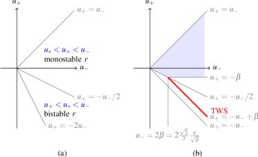
Figure 3: a) classification of reaction function $r$ depending on its roots $u_{-}$, $u_{+}$ and $u_{*}=-u_{-}-u_{+}$; b) Endstates $u_{\pm}$ in the shaded region and on the thick line can be connected by TWS of the cubic KdVB equation; TWS in the shaded region and on the thick line are associated to classical and non-classical shocks of $\partial_{t}{u}+\partial_{x}{u^{3}}=0$, respectively. For a classical shock the shock triple satisfies Lax’ entropy condition $f^{\prime}(u_{-})>c>f^{\prime}(u_{+})$; i.e. characteristics in the Riemann problem meet at the shock. In contrast, the non-classical shocks are of slow undercompressive type, i.e. characteristics in the Riemann problem cross the shock.

4 TWP for nonlocal evolution equations

4.1 reaction-diffusion equations

The first example of a reaction-diffusion equation with nonlocal diffusion is the integro-differential equation

$$\partial_{t}{u}=J\ast u-u+r(u)\ ,\quad t>0\ ,\quad x\in\mathbb{R}\ ,$$ (35)

for some even, non-negative function $J$ with mass one, i.e. for all $x\in\mathbb{R}$

$$J\in C(\mathbb{R})\ ,\quad J\geq 0\ ,\quad J(x)=J(-x)\ ,\quad\int_{\mathbb{R}}\;{J(y)}\;\,\operatorname{d}\!y\,=1\ ,$$ (36)

and some function $r$. The operator $\mathcal{L}[u]=J\ast u-u$ is a Lévy operator, see (13), which models nonlocal diffusion. It is the infinitesimal generator of a compound Poisson stochastic process, which is a pure jump process.

The TWP for given endstates $u_{\pm}$ is to study the existence of a TWS $(\bar{u},c)$ for (35) in the sense of Definition 1. Such a TWS $(\bar{u},c)$ satisfies the TWE $-c\bar{u}^{\prime}=J\ast\bar{u}-\bar{u}+r(\bar{u})$ for $\xi\in\mathbb{R}$. Next, we recall some results on the TWP for (35), which will depend crucially on the type of reaction function $r$ and the tail behavior of a kernel function $J$. We will present the existence of TWS with monotone decreasing profiles $\bar{u}$, which will follow from the cited literature after a suitable transformation.

Proposition 6 ((monostable [21]), (bistable [11, 19])).

Suppose $u_{-}>u_{+}$ and consider reaction functions $r$ in the sense of Definition 4. Suppose $J\in W^{1,1}(\mathbb{R})$ and its continuous representative satisfies (36).

• If $r$ is monostable and there exists $\lambda>0$ such that $\int_{\mathbb{R}}\;{J(y)\ \exp(\lambda y)}\;\,\operatorname{d}\!y\,<\infty$ then there exists a positive constant $c_{*}$ such that for all $c\geq c_{*}$ there exists a monotone TWS $(\bar{u},c)$ of (35). For $c<c_{*}$ no such monotone TWS exists.

• If $r$ is bistable and $\int_{\mathbb{R}}\;{|y|J(y)}\;\,\operatorname{d}\!y\,<\infty$, then there exists an (up to translations) unique monotone TWS $(\bar{u},c)$ of (35).

For monostable reaction functions, the tail behavior of kernel function $J$ is very important. There exist kernel functions $J$, such that TWS exist only for bistable – but not for monostable – reaction functions $r$, see [47]. The prime example are kernel functions $J$ which decay more slowly than any exponentially decaying function as $|x|\to\infty$ in the sense that $J(x)\exp(\eta|x|)\to\infty$ as $|x|\to\infty$ for all $\eta>0$.

For reaction-diffusion equations of bistable type, Chen established a unified approach [19] to prove the existence, uniqueness and asymptotic stability with exponential decay of traveling wave solutions. The results are established for a subclass of nonlinear nonlocal evolution equations

$$\partial_{t}{u}(x,t)=\mathcal{A}[u(\cdot,t)](x)\quad\text{ for }\,(x,t)\in\mathbb{R}\times(0,T]\ ,$$

where the nonlinear operator $\mathcal{A}$ is assumed to

1. be independent of $t$;

2. generate a $L^{\infty}$ semigroup;

3. be translational invariant, i.e. $\mathcal{A}$ satisfies for all $u\in\operatorname{dom}\mathcal{A}$ the identity

   $$\mathcal{A}[u(\cdot+h)](x)=\mathcal{A}[u(\cdot)](x+h)\quad\forall x\ ,h\in\mathbb{R}\,.$$

   Consequently, there exists a function $r:\mathbb{R}\to\mathbb{R}$ which is defined by $\mathcal{A}[\upsilon\mathbf{1}]=r(\upsilon)\mathbf{1}$ for $\upsilon\in\mathbb{R}$ and the constant function $\mathbf{1}:\mathbb{R}\to\mathbb{R}$, $x\mapsto 1$. This function $r$ is assumed to be bistable in the sense of Definition 4;

4. satisfy a comparison principle: If $\partial_{t}{u}\geq\mathcal{A}[u]$, $\partial_{t}{v}\leq\mathcal{A}[v]$ and $u(\cdot,0)\gneq v(\cdot,0)$, then $u(\cdot,t)>v(\cdot,t)$ for all $t>0$.

Chen’s approach relies on the comparison principle and the construction of sub- and supersolutions for any given traveling wave solution. Importantly, the method does not depend on the balance of the potential. More quantitative versions of the assumptions on $\mathcal{A}$ are needed in the proofs. Finally integro-differential evolution equations

$$\partial_{t}{u}=\epsilon\partial^{2}_{x}{u}+G(u,J_{1}\ast S^{1}(u),\ldots,J_{n}\ast S^{n}(u))$$ (37)

are considered for some diffusion constant $\epsilon\geq 0$, smooth functions $G$ and $S^{k}$, and kernel functions $J_{k}\in C^{1}(\mathbb{R})\cap W^{1,1}(\mathbb{R})$ satisfying (36) where $k=1,\ldots,n$. Additional assumptions on the model parameters guarantee that an equation (37) can be interpreted as a reaction-diffusion equation with bistable reaction function including equations (20) and (35) as special cases.

Another example of reaction-diffusion equations with nonlocal diffusion are the integro-differential equations

$$\partial_{t}{u}=D^{a}_{\theta}u+r(u)\ ,\quad t>0\ ,\quad x\in\mathbb{R}\ ,$$ (38)

for a (particle) density $u=u(x,t)$, some function $r=r(u)$, and a Riesz-Feller operator $D^{a}_{\theta}$ with $(\alpha,\theta)\in\mathfrak{D}_{a,\theta}$. The nonlocal Riesz-Feller operators are models for superdiffusion, where from a probabilistic view point a cloud of particle is assumed to spread faster than by following Brownian motion. Integro-differential equation (38) can be derived as a macroscopic equation for a particle density in the limit of modified Continuous Time Random Walk (CTRW), see [37]. In the applied sciences, equation (38) has found many applications, see [43, 46] for extensive reviews on modeling, formal analysis and numerical simulations.

The TWP for given endstates $u_{\pm}$ is to study the existence of a TWS $(\bar{u},c)$ for (38) in the sense of Definition 1. Such a TWS $(\bar{u},c)$ satisfies the TWE

$$-c\bar{u}^{\prime}=D^{a}_{\theta}\bar{u}+r(\bar{u})\ ,\quad\xi\in\mathbb{R}\ .$$ (39)

First we collect mathematical rigorous results about the TWP associated to (38) in case of the fractional Laplacian $D^{a}_{0}=-(-\Delta)^{a/2}$ for $a\in(0,2)$, i.e. a Riesz-Feller operator $D^{a}_{\theta}$ with $\theta=0$.

Proposition 7 ((monostable [13, 14, 24]), (bistable [17, 15, 16, 39, 20, 27])).

Suppose $u_{-}>u_{+}$. Consider the TWP for reaction-diffusion equation (38) with functions $r$ in the sense of Definition 4 and fractional Laplacian $D^{a}_{0}$, i.e. symmetric Riesz-Feller operators $D^{a}_{\theta}$ with $0<a<2$ and $\theta=0$.

• If $r$ is monostable then there does not exist any TWS $(\bar{u},c)$ of (38).

• If $r$ is bistable then there exists an (up to translations) unique monotone TWS $(\bar{u},c)$ of (38).

For monostable reaction functions, Cabré and Roquejoffre prove that a front moves exponentially in time [13, 14]. They note that the genuine algebraic decay of the heat kernels $G^{a}_{0}$ associated to fractional Laplacians is essential to prove the result, which implies that no TWS with constant wave speed can exist. Engler [24] considered the TWP for (38) for a different class of monostable reaction functions $r$ and non-extremal Riesz-Feller operators $D^{a}_{\theta}$ with $(a,\theta)\in\mathfrak{D}_{a,\theta}^{+}$ and $\mathfrak{D}_{a,\theta}^{+}:=\{\,{(a,\theta)\in\mathfrak{D}_{a,\theta}}\,|\,{|\theta|<\min\{a,2-a\}}\,\}$. Again the associated heat kernels $G^{a}_{\theta}(x,t)$ with $(a,\theta)\in\mathfrak{D}_{a,\theta}^{+}$ decay algebraically in the limits $x\to\pm\infty$, see [36].

To our knowledge, we established the first result [6] on existence, uniqueness (up to translations) and stability of traveling wave solutions of (38) with Riesz-Feller operators $D^{a}_{\theta}$ for $(a,\theta)\in\mathfrak{D}_{a,\theta}$ with $1<a<2$ and bistable functions $r$. We present our results for monotone decreasing profiles, which can be inferred from our original result after a suitable transformation.

Theorem 3 ([6]).

Suppose $u_{-}>u_{+}$, $(a,\theta)\in\mathfrak{D}_{a,\theta}$ with $1<a<2$, and $r\in C^{\infty}(\mathbb{R})$ is a bistable reaction function. Then there exists an (up to translations) unique monotone decreasing TWS $(\bar{u},c)$ of (38) in the sense of Definition 1.

The technical details of the proof are contained in [6], whereas in [5] we give a concise overview of the proof strategy and visualize the results also numerically. In a forthcoming article [4], we extend the results to all non-trivial Riesz-Feller operators $D^{a}_{\theta}$ with $(a,\theta)\in\mathfrak{D}_{a,\theta}^{\diamond}$. The smoothness assumption on $r$ is convenient, but not essential. To prove Theorem 3, we follow – up to some modifications – the approach of Chen [19]. It relies on a strict comparison principle and the construction of sub- and supersolutions for any given TWS. His quantitative assumptions on operator $\mathcal{A}$ are too strict, such that his results are not directly applicable. A modification allows to cover the TWP for (38) for all Riesz-Feller operators $D^{a}_{\theta}$ with $1<a<2$ also for non-zero $\theta$, and all bistable functions $r$ regardless of the balance of the potential.

Next, we quickly review different methods to study the TWP of reaction-diffusion equations (38) with bistable function $r$ and fractional Laplacian. In case of a classical reaction-diffusion equation (20), the existence of a TWS can be studied via phase-plane analysis [10, 25]. This method has no obvious generalization to our TWP for (38), since its traveling wave equation (39) is an integro-differential equation. The variational approach has been focused – so far – on symmetric diffusion operators such as fractional Laplacians and on balanced potentials, hence covering only stationary traveling waves [39]. Independently, the same results are achieved in [17, 15, 16] by relating the stationary TWE (39)_θ=0,c=0 via [18] to a boundary value problem for a nonlinear partial differential equation. The homotopy to a simpler TWP has been used to prove the existence of TWS in case of (35), and (38)_θ=0 with unbalanced potential [27].

Chmaj [20] also considers the TWP for (38)_θ=0 with general bistable functions $r$. He approximates a given fractional Laplacian by a family of operators $J_{\epsilon}\ast u-(\int J_{\epsilon})u$ such that $\lim_{\epsilon\to 0}J_{\epsilon}\ast u-(\int J_{\epsilon})u=D^{a}_{0}u$ in an appropriate sense. This allows him to obtain a TWS of (38)_θ=0 with general bistable function $r$ as the limit of the TWS $u_{\epsilon}$ of (35) associated to $(J_{\epsilon})_{\epsilon\geq 0}$. It might be possible to modify Chmaj’s approach to study reaction-diffusion equation (38) with asymmetric Riesz-Feller operators. This would give an alternative existence proof for TWS in Theorem 3. However, Chen’s approach allows to establish uniqueness (up to translations) and stability of TWS as well.

4.2 nonlocal Korteweg-de Vries-Burgers equation

First we consider the integro-differential equation in multi-dimensions $d\geq 1$

$$\partial_{t}{u}+\partial_{x}{f(u)}=\epsilon\Delta_{x}u+\gamma\epsilon^{2}\sum_{j=1}^{d}\big{(}\phi_{\epsilon}\ast\partial_{x_{j}}{u}-\partial_{x_{j}}{u}\big{)}\ ,\quad x\in\mathbb{R}^{d}\ ,\quad t>0\ ,$$ (40)

for parameters $\epsilon>0$, $\gamma\in\mathbb{R}$, a smooth even non-negative function $\phi$ with compact support and unit mass, i.e. $\int_{\mathbb{R}^{d}}\;{\phi(x)}\;\,\operatorname{d}\!x\,=1$, and the rescaled kernel function $\phi_{\epsilon}(x)=\phi(x/\epsilon)/\epsilon^{d}$. It has been derived as a model for phase transitions with long range interactions close to the surface, which supports planar TWS associated to undercompressive shocks of (51), see [41]. A planar TWS $(\bar{u},c)$ is a solution $u(x,t)=\bar{u}(x-cte)$ for some fixed vector $e\in\mathbb{R}^{d}$, such that the profile is transported in direction $e$. The existence of planar TWS is proven by reducing the problem to a one-dimensional TWP for (40)_d=1, identifying the associated reaction-diffusion equation (35) and using results in Proposition 6. For cubic flux function $u^{3}$, the existence of planar TWS associated to undercompressive shocks of (51) is established. Moreover, the well-posedness of its Cauchy problem and the convergence of solutions $u^{\epsilon}$ as $\epsilon\searrow 0$ have been studied [41].

Another example is the fractal Korteweg-de Vries-Burgers equation

$$\partial_{t}{u}+\partial_{x}{f(u)}=\epsilon\partial_{x}{}\mathcal{D}^{\alpha}_{+}u+\delta\partial^{3}_{x}{u},\quad x\in\mathbb{R},\quad t>0,$$ (41)

for some $\epsilon>0$ and $\delta\in\mathbb{R}$.

Equation (41) with $\alpha=1/3$ has been derived as a model for shallow water flows, by performing formal asymptotic expansions associated to the triple-deck (boundary layer) theory in fluid mechanics, e.g. see [33, 44]. In particular, the situations of one-layer and two-layer shallow water flows have been considered, which yield a quadratic (one layer) and cubic flux function (two layer), respectively. In the monograph [38], similar models are considered and the well-posedness of the initial value problem and possible wave-breaking are studied.

The TWP for given endstates $u_{\pm}$ is to study the existence of a TWS $(\bar{u},c)$ for (41) in the sense of Definition 1. Such a TWS $(\bar{u},c)$ satisfies the TWE

$$h(\bar{u}):=f(\bar{u})-f(u_{-})-c(\bar{u}-u_{-})=\epsilon\mathcal{D}^{\alpha}_{+}\bar{u}+\delta\bar{u}^{\prime\prime}\ .$$ (42)

We obtain a necessary condition for the existence of TWS – see also (25) – by multiplying the TWE with $\bar{u}^{\prime}$ and integrating on $\mathbb{R}$,

$$\int_{u_{-}}^{u_{+}}\;{h(u)}\;\,\operatorname{d}\!u\,=\epsilon\int_{-\infty}^{\infty}\;{\bar{u}^{\prime}\ \mathcal{D}^{\alpha}_{+}\bar{u}(\xi)}\;\,\operatorname{d}\!\xi\,\geq 0\ ,$$ (43)

where the last inequality follows from (50).

connection with reaction-diffusion equation. If a TWS $(\bar{u},c)$ for (41) exists, then $u(x,t)=\bar{u}(x)$ is a stationary TWS $(\bar{u},0)$ of the evolution equation

$$\partial_{t}{u}=-\epsilon\mathcal{D}^{\alpha}_{+}u-\delta\partial^{2}_{x}{u}+h(u),\quad x\in\mathbb{R},\quad t>0.$$ (44)

To interpret equation (44) as a reaction-diffusion equation, we need to verify that $-\epsilon\mathcal{D}^{\alpha}_{+}u-\delta\partial^{2}_{x}{u}$ is a diffusion operator, e.g. that $-\epsilon\mathcal{D}^{\alpha}_{+}u-\delta\partial^{2}_{x}{u}$ generates a positivity preserving semigroup.

Lemma 4.

Suppose $0<\alpha<1$ and $\gamma_{1},\gamma_{2}\in\mathbb{R}$. The operator $\gamma_{1}\mathcal{D}^{\alpha}_{+}u+\gamma_{2}\partial^{2}_{x}{u}$ is a Lévy operator if and only if $\gamma_{1}\leq 0$ and $\gamma_{2}\geq 0$. Moreover, the associated heat kernel is strictly positive if and only if $\gamma_{2}>0$.

Proof.

For $\alpha\in(0,1)$, the operator $-\mathcal{D}^{\alpha}_{+}$ is a Riesz-Feller operator $D^{\alpha}_{-\alpha}$ and generates a positivity preserving convolution semigroup with a Lévy stable probability distribution $G^{\alpha}_{-\alpha}$ as its kernel. The probability distribution is absolutely continuous with respect to Lebesgue measure and its density has support on a half-line [36]. For example the kernel associated to $-\mathcal{D}^{1/2}$ is the Lévy-Smirnov distribution. Thus, for $\gamma_{1}\leq 0$ and $\gamma_{2}\geq 0$, the operator $\gamma_{1}\mathcal{D}^{\alpha}_{+}u+\gamma_{2}\partial^{2}_{x}{u}$ is a Lévy operator, because it is a linear combination of Lévy operators. Using the notation for Fourier symbols of Riesz-Feller operators, the partial Fourier transform of equation

$$\partial_{t}{u}=-|\gamma_{1}|\mathcal{D}^{\alpha}[u]+\gamma_{2}\partial^{2}_{x}{u}$$

is given by $\partial_{t}{}\mathcal{F}[u](k)=(|\gamma_{1}|\psi^{\alpha}_{-\alpha}(k)-\gamma_{2}k^{2})\mathcal{F}[u](k)$. Therefore, the operator generates a convolution semigroup with heat kernel

$$\mathcal{F}^{-1}[\exp\{(|\gamma_{1}|\psi^{\alpha}_{-\alpha}(k)-\gamma_{2}k^{2})\ t\}](x)=G^{\alpha}_{-\alpha}(\cdot,|\gamma_{1}|t)\ast G^{2}_{0}(\cdot,\gamma_{2}t)\ (x)\ ,$$

which is the convolution of two probability densities. The kernel is positive on $\mathbb{R}$ since probability densities are non-negative on $\mathbb{R}$ and the normal distribution $G^{2}_{0}$ is positive on $\mathbb{R}$ for positive $\gamma_{2}t$.

The operator $\mathcal{D}^{\alpha}_{+}$ for $\alpha\in(0,1)$ is not a Riesz-Feller operator, see Figure 1, and it generates a semigroup which is not positivity preserving. Thus it and any linear combination with $\gamma_{1}>0$ is not a Lévy operator.

∎∎

convex flux functions.

Proposition 8.

Consider (41) with $0<\alpha<1$, $\delta\in\mathbb{R}$ and strictly convex flux function $f\in C^{3}(\mathbb{R})$. For a shock triple $(u_{-},u_{+};c)$ satisfying the Rankine-Hugoniot condition (54), a non-constant TWS $(\bar{u},c)$ can exist if and only if Lax’ entropy condition (55) is fulfilled, i.e. $u_{-}>u_{+}$.

Proof.

The Rankine-Hugoniot condition (54) ensures that $h(u)$ in (42) has exactly two roots $u_{\pm}$. If Lax’ entropy condition (55) is fulfilled, then $u_{-}>u_{+}$ and $-h(u)$ is monostable in the sense of Definition 4. Thus, the necessary condition (43) is satisfied. If $u_{-}=u_{+}$ then (43) implies that $\bar{u}$ is a constant function satisfying $\bar{u}\equiv u_{\pm}$. If $u_{-}<u_{+}$ then $-h(u)$ is monostable in the sense of Definition 4 with reversed roles of $u_{\pm}$. Thus, the necessary condition (43) is not satisfied.

∎∎

Next, we recall some existence result which have been obtained by directly studying the TWE. In an Addendum [22], we removed an initial assumption on the solvability of the linearized TWE.

Theorem 5 ([3]).

Consider (41) with $\delta=0$ and convex flux function $f(u)$. For a shock triple $(u_{-},u_{+};c)$ satisfying (54) and (55), there exists a monotone TWS of (41) in the sense of Definition 1, whose profile $\bar{u}\in C^{1}_{b}(\mathbb{R})$ is unique (up to translations) among all functions $u\in u_{-}+H^{2}(-\infty,0)\cap C^{1}_{b}(\mathbb{R})$.

This positive existence result is consistent with the negative existence result in Proposition 7 and Engler [24] for (38) with non-extremal Riesz-Feller operators $D^{a}_{\theta}$ for $(a,\theta)\in\mathfrak{D}_{a,\theta}^{+}$. The reason is that $-\mathcal{D}^{\alpha}_{+}$ for $0<\alpha<1$ is the generator of a convolution semigroup with a one-sided strictly stable probability density function as its heat kernel; in contrast to heat kernels with genuine algebraic decay [13, 14, 24].

Theorem 6 ([2]).

Consider (41) with flux function $f(u)=u^{2}/2$. For a shock triple $(u_{-},u_{+};c)$ satisfying (54) and (55), there exists a TWS of (41) in the sense of Definition 1, whose profile $\bar{u}$ is unique (up to translations) among all functions $u\in u_{-}+H^{4}(-\infty,0)\cap C^{3}_{b}(\mathbb{R})$.

If dispersion dominates diffusion then the profile of a TWS $(\bar{u},c)$ will be oscillatory in the limit $\xi\to\infty$. For a classical KdVB equation this geometry of profiles depends on the ratio $\epsilon^{2}/\delta$ and the threshold can be determined explicitly.

concave-convex flux functions. We consider a cubic flux function $f(u)=u^{3}$ as the prototypical concave-convex flux function. Again the necessary condition (43) and the classification of function $h(u)=-r(u)$ in Figure 2 can be used to identify non-admissible shock triples $(u_{-},u_{+};c)$ for the TWP of (41).

We conjecture that a statement analogous to Proposition 5 holds true. Of special interest is again the occurrence of TWS $(\bar{u},c)$ associated to non-classical shocks, which are only expected in case of (41) with $\epsilon>0$ and $\delta>0$.

Proposition 9 (conjecture).

Suppose $f(u)=u^{3}$ and $\epsilon>0$.

1. If $\delta\leq 0$ then a TWS $(\bar{u},c)$ of (41) exists if and only if $(u_{-},u_{+};c)$ satisfy the Rankine-Hugoniot condition (54) and the entropy condition (55).

2. If $\delta>0$ then a TWS $(\bar{u},c)$ of (41) exists for $u_{-}>0$ if and only if $u_{+}\in S(u_{-})$ for some set $S(u_{-})$ similar to (33).

sketch of proof.

If $\delta=0$, then equation (41) is a viscous conservation law, and its TWE (42) is a fractional differential equation $\epsilon\mathcal{D}^{\alpha}_{+}\bar{u}=h(\bar{u})$. Thus a heteroclinic orbit exists only for monostable $-h(u)$, i.e. if the unstable node $u_{-}$ and the stable node $u_{+}$ are not separated by any other root of $h$. This follows from Theorem 5 and its proof in [3, 22].

If $\delta<0$, then the TWE (42) is associated to a reaction-diffusion equation (44) via a stationary TWS ansatz $u(x,t)=\bar{u}(x)$. First we note that a stronger version of the necessary condition (43) is available

$$\int_{-\infty}^{\xi}\;{h(\bar{u})\bar{u}^{\prime}(y)}\;\,\operatorname{d}\!y\,=\epsilon\int_{-\infty}^{\xi}\;{\bar{u}^{\prime}\ \mathcal{D}^{\alpha}_{+}\bar{u}(y)}\;\,\operatorname{d}\!y\,\geq 0\ ,\quad\forall\xi\in\mathbb{R}\ ,$$ (45)

see [2]. If $u_{+}<u_{*}<u_{-}$ then $h(u)$ is an unstable reaction function, see Figure 2. Thus there exists no TWS in the sense of Definition 1 satisfying the necessary condition (45). If $u_{*}<u_{+}<u_{-}$ then function $-h(u)$ is monostable in the sense of Definition 4 and the necessary condition (43) can be satisfied. The existence of a TWS $(\bar{u},c)$ can be proven by following the analysis in [2, 22]. The TWP for other pairs $(u_{-},u_{+})$ is discussed similarly.

If $\delta>0$ then the occurrence of TWS $(\bar{u},c)$ associated to non-classical shocks is possible. Unlike in our previous examples, the associated evolution equation (44) is not a reaction-diffusion equation, since $-\epsilon\mathcal{D}^{\alpha}_{+}\bar{u}-\delta\bar{u}^{\prime\prime}$ is not a Lévy operator. Especially, the results on existence of TWS for reaction-diffusion equations with bistable reaction function can not be used to prove the existence of TWS $(\bar{u},c)$ associated to a undercompressive shocks. Instead, we investigate the TWP directly [1], extending the analysis in [2, 22] for Burgers’ flux to the cubic flux function $f(u)=u^{3}$.

∎∎

4.3 Fowler’s equation

Fowler’s equation (8) for dune formation is a special case of the evolution equation

$$\partial_{t}{u}+\partial_{x}{f(u)}=\delta\partial^{2}_{x}{}u-\epsilon\partial_{x}{}\mathcal{D}^{\alpha}_{+}u\ ,\quad t>0\ ,\quad x\in\mathbb{R}\ ,$$ (46)

with $0<\alpha<1$, positive constant $\epsilon,\delta>0$ and flux function $f$. Here the fractional derivative appears with the negative sign, but this instability is regularized by the second order derivative. The initial value problem for (8) is well-posed in $L^{2}$ [7]. However, it does not support a maximum principle, which is intuitive in the context of the application due to underlying erosions [7]. The existence of TWS of (8) – without assumptions (3) on the far-field behavior – has been proven [8].

For given endstates $u_{\pm}$, the TWP for (46) is to study the existence of a TWS $(\bar{u},c)$ for (46) in the sense of Definition 1. Such a TWS $(\bar{u},c)$ satisfies the TWE

$$h(\bar{u}):=f(\bar{u})-f(u_{-})-c(\bar{u}-u_{-})=\delta\bar{u}^{\prime}-\epsilon\mathcal{D}^{\alpha}_{+}\bar{u}\ ,\quad\xi\in\mathbb{R}\ .$$ (47)

For $\delta=0$, the TWE reduces to a fractional differential equation $\epsilon\mathcal{D}^{\alpha}_{+}\bar{u}=-h(\bar{u})$, which has been analyzed in [3, 22] for monostable functions $-h(u)$.

Equation (47) is also the TWE for a TWS $(\bar{u},\delta)$ of an evolution equation

$$\partial_{t}{u}=-\epsilon\mathcal{D}^{\alpha}_{+}u-h(u),\quad x\in\mathbb{R},\quad t>0.$$ (48)

For $\epsilon>0$, the operator is $-\epsilon\mathcal{D}^{\alpha}_{+}\bar{u}$ is a Riesz-Feller operator $\epsilon D^{\alpha}_{-\alpha}$ whose heat kernel $G^{\alpha}_{-\alpha}$ has only support on a halfline. For a shock triple $(u_{-},u_{+};c)$ satisfying the Rankine-Hugoniot condition (54), at least $h(u_{\pm})=0$ holds. Under these assumptions, equation (48) is a reaction-diffusion equation with a Riesz-Feller operator modeling diffusion.

The abstract method in [8] does not provide any information on the far-field behavior. Thus, assume the existence of a TWS $(\bar{u},c)$ in the sense of Definition 1, for some shock triple $(u_{-},u_{+};c)$ satisfying the Rankine-Hugoniot condition (54). Again, a necessary condition is obtained by multiplying TWE (47) with $\bar{u}^{\prime}$ and integrating on $\mathbb{R}$; hence,

$$\int_{u_{-}}^{u_{+}}\;{h(u)}\;\,\operatorname{d}\!u\,=\int_{\mathbb{R}}\;{(\bar{u}^{\prime})^{2}}\;\,\operatorname{d}\!\xi\,-\int_{\mathbb{R}}\;{\bar{u}^{\prime}\mathcal{D}^{\alpha}_{+}\bar{u}}\;\,\operatorname{d}\!\xi\,\ .$$ (49)

The left hand side is indefinite since each integral is non-negative, see also (50).

For a cubic flux function $f(u)=u^{3}$ and a shock triple $(u_{-},u_{+};c)$ satisfying the Rankine-Hugoniot condition (54), we deduce a bistable reaction function $r(u)=-h(u)$ as long as $u_{+}<-u_{+}-u_{-}<u_{-}$ see Figure 2. However, since the heat kernel has only support on a halfline, we can not obtain a strict comparison principle as needed in Chen’s approach [19, 6, 4].

Appendix A Caputo fractional derivative on $\mathbb{R}$

For $\alpha>0$, the (Gerasimov-)Caputo derivatives are defined as, see [32, 43],

$$(\mathcal{D}^{\alpha}_{+}f)(x) =\begin{cases}f^{(n)}(x)&\text{if }\alpha=n\in\mathbb{N}_{0}\ ,\\ \tfrac{1}{\Gamma(n-\alpha)}\int_{-\infty}^{x}\;{\frac{f^{(n)}(y)}{(x-y)^{\alpha-n+1}}}\;\,\operatorname{d}\!y\,&\text{if }n-1<\alpha<n\text{ for some }n\in\mathbb{N}_{0}\ .\end{cases}$$

$$(\mathcal{D}^{\alpha}_{-}f)(x) =\begin{cases}f^{(n)}(x)&\text{if }\alpha=n\in\mathbb{N}_{0}\ ,\\ \tfrac{(-1)^{n}}{\Gamma(n-\alpha)}\int_{x}^{\infty}\;{\frac{f^{(n)}(y)}{(y-x)^{\alpha-n+1}}}\;\,\operatorname{d}\!y\,&\text{if }n-1<\alpha<n\text{ for some }n\in\mathbb{N}_{0}\ .\end{cases}$$

properties:

• For $\alpha>0$ and $\lambda>0$

  $$(\mathcal{D}^{\alpha}_{+}\exp(\lambda\cdot))(x)=\lambda^{\alpha}\exp(\lambda x)\ ,\quad(\mathcal{D}^{\alpha}_{-}\exp(-\lambda\cdot))(x)=\lambda^{\alpha}\exp(-\lambda x)$$

• For $\alpha>0$ and $f\in\mathcal{S}(\mathbb{R})$, a Caputo derivative is a Fourier multiplier operator with $(\mathcal{F}\mathcal{D}^{\alpha}_{+}f)(k)=(\operatorname{i}k)^{\alpha}(\mathcal{F}f)(k)$ where $(\operatorname{i}k)^{\alpha}=\exp(\alpha\pi\operatorname{i}\operatorname{sgn}(k)/2)$.

• If $\bar{u}$ is the profile of a TWS $(\bar{u},c)$ in the sense of Definition 1, then

  $$\int_{-\infty}^{\infty}\;{\bar{u}^{\prime}(y)\,\mathcal{D}^{\alpha}_{+}\bar{u}(y)}\;\,\operatorname{d}\!y\,=\tfrac{1}{2}\int_{\mathbb{R}}\;{\bar{u}^{\prime}(x)\int_{\mathbb{R}}\;{\frac{\bar{u}^{\prime}(y)}{|x-y|^{\alpha}}}\;\,\operatorname{d}\!y\,}\;\,\operatorname{d}\!x\,\geq 0\ ,$$ (50)

  where the last inequality follows from [35, Theorem 9.8].

Appendix B shock wave theory for scalar conservation laws

A standard reference on the theory of conservation laws is [23], whereas [34] covers the special topic of non-classical shock solutions. A scalar conservation law is a partial differential equation

$$\partial_{t}{u}+\partial_{x}{f(u)}=0\ ,\quad t>0\ ,\quad x\in\mathbb{R}\ ,$$ (51)

for some flux function $f:\mathbb{R}\to\mathbb{R}$. For nonlinear functions $f$, it is well known that the initial value problem (IVP) for (51) with smooth initial data may not have a classical solution for all time $t>0$ (due to shock formation). However, weak solutions may not be unique. The Riemann problems are a subclass of IVPs for (51), and especially important in some numerical algorithms: For given $u_{-},u_{+}\in\mathbb{R}$, find a weak solution $u(x,t)$ for the initial value problem of (51) with initial condition

$$u(x,0)=\begin{cases}u_{-}\ ,&x<0\ ,\\ u_{+}\ ,&x>0\,.\end{cases}$$ (52)

Weak solutions of a Riemann problem that are discontinuous for $t>0$ may not be unique.

Example 1.

A shock wave is a discontinuous solution of the Riemann problem,

$$u(x,t)=\begin{cases}u_{-}\ ,&x<ct\ ,\\ u_{+}\ ,&x>ct\ ,\end{cases}$$ (53)

if the shock triple $(u_{-},u_{+};c)$ satisfies the Rankine-Hugoniot condition

$$f(u_{+})-f(u_{-})=c(u_{+}-u_{-})\,.$$ (54)

The Rankine-Hugoniot condition (54) is a necessary condition that $u_{\pm}$ are stationary states of an associated TWE (28), see (30).

shock admissibility

Classical approaches to select a unique weak solution of the Riemann problem are

1. Lax’ entropy condition:

   $$f^{\prime}(u_{+})<c<f^{\prime}(u_{-})\ .$$ (55)

   It ensures that in the method of characteristics all characteristics enter the shock/discontinuity of a shock solution (53). For convex flux function $f$, condition (55) reduces to $u_{-}>u_{+}$. Shocks satisfying (55) are also called Lax or classical shocks. For non-convex flux functions $f$, also non-classical shocks can arise in experiments, called slow undercompressive shocks if $f^{\prime}(u_{\pm})>c$, and fast undercompressive shocks if $f^{\prime}(u_{\pm})<c$.

2. Oleinik’s entropy condition.

   $$\frac{f(w)-f(u_{-})}{w-u_{-}}\geq\frac{f(u_{+})-f(u_{-})}{u_{+}-u_{-}}\quad\text{ for all $w$ between $u_{-}$ and $u_{+}$. }\quad$$ (56)

3. entropy solutions satisfying integral inequalities based on entropy-entropy flux pairs, such as Kruzkov’s family of entropy-entropy flux pairs.

4. vanishing viscosity. In the classical vanishing viscosity approach, instead of (51) one considers for $\epsilon>0$ equation

   $$\partial_{t}{u}+\partial_{x}{f(u)}=\epsilon\partial^{2}_{x}{u}\ ,\quad t>0\ ,\quad x\in\mathbb{R}\ ,$$ (57)

   where $\epsilon\partial^{2}_{x}{u}$ models diffusive effects such as friction. Equation (57) is a parabolic equation, hence the Cauchy problem has global smooth solutions $u^{\epsilon}$ for positive times, especially for Riemann data (52). An admissible weak solution of the Riemann problem is identified by studying the limit of $u^{\epsilon}$ as $\epsilon\searrow 0$.
   In other applications, different higher order effects may be important. For example, a nonlocal generalized KdVB equation (1) can be interpreted as a scalar conservation law (51) with higher-order effects $\mathcal{R}[u]:=\epsilon\mathcal{L}_{1}[u]+\delta\partial_{x}{}\mathcal{L}_{2}[u]$.
   

   Already for convex functions $f$, the convergence of solutions of the regularized equations (e.g. (1)) to solutions of (51) reveals a diverse solution structure. The solutions of viscous conservation laws (57) converge for $\epsilon\searrow 0$ to Kruzkov entropy solutions of (51). In contrast, in case of KdVB equation (4) the limit $\epsilon,\delta\to 0$ depends on the relative strength of diffusion and dispersion:

   • weak dispersion $\delta=O(\epsilon^{2})$ for $\epsilon\to 0$ e.g. $\delta=\beta\epsilon^{2}$ for some $\beta>0$.
     TWS converge strongly to entropy solution of Burgers equation.

   • moderate dispersion $\delta=o(\epsilon)$ for $\epsilon\to 0$ includes weak dispersion.
     TWS converge strongly to entropy solution of Burgers equation, see [40].

   • strong dispersion weak limit of TWS for $\epsilon,\delta\to 0$ may not be a weak solution of Burgers equation.

   For non-convex flux functions $f$, a TWS may converge to a weak solution of (51) which is not an Kruzkov entropy solution, but a non-classical shock.

A simplistic shock admissibility criterion based on the vanishing viscosity approach is the existence of TWS for a given shock triple:

Definition 6 (compare with [31]).

A solution $u$ of the Riemann problem is called admissible (with respect to a fixed regularization $\mathcal{R}$), if there exists a TWS $(\bar{u},c)$ in the sense of Definition 1 of the regularized equation (e.g. (1)) for every shock wave with shock triple $(u_{-},u_{+};c)$ in the solution $u$.

References

- [1] F. Achleitner and C. M. Cuesta. Non-classical shocks in a non-local generalised Korteweg-de Vries-Burgers equation. work in progress.
- [2] F. Achleitner, C. M. Cuesta, and S. Hittmeir. Travelling waves for a non-local Korteweg–de Vries–Burgers equation. J. Differential Equations, 257(3):720–758, 2014.
- [3] F. Achleitner, S. Hittmeir, and C. Schmeiser. On nonlinear conservation laws with a nonlocal diffusion term. J. Differential Equations, 250(4):2177–2196, 2011.
- [4] F. Achleitner and C. Kuehn. Traveling waves for a bistable reaction-diffusion equation with nonlocal Riesz-Feller operator. work in progress.
- [5] F. Achleitner and C. Kuehn. Analysis and numerics of traveling waves for asymmetric fractional reaction-diffusion equations. Commun. Appl. Ind. Math., 6(2):e–532, 25, 2015.
- [6] F. Achleitner and C. Kuehn. Traveling waves for a bistable equation with nonlocal diffusion. Adv. Differential Equations, 20(9-10):887–936, 2015.
- [7] N. Alibaud, P. Azerad, D. Isèbe, et al. A non-monotone nonlocal conservation law for dune morphodynamics. Differential and Integral Equations, 23(1/2):155–188, 2010.
- [8] B. Alvarez-Samaniego and P. Azerad. Existence of travelling-wave solutions and local well-posedness of the Fowler equation. Discrete Contin. Dyn. Syst. Ser. B, 12(4):671–692, 2009.
- [9] D. Applebaum. Lévy processes and stochastic calculus, volume 116 of Cambridge Studies in Advanced Mathematics. Cambridge University Press, Cambridge, second edition, 2009.
- [10] D. G. Aronson and H. F. Weinberger. Nonlinear diffusion in population genetics, combustion, and nerve pulse propagation. In Partial differential equations and related topics, pages 5–49. Lecture Notes in Math., Vol. 446. Springer, Berlin, 1975.
- [11] P. W. Bates, P. C. Fife, X. Ren, and X. Wang. Traveling waves in a convolution model for phase transitions. Archive for Rational Mechanics and Analysis, 138:105–136, 1997.
- [12] J. L. Bona and M. E. Schonbek. Travelling-wave solutions to the Korteweg-de Vries-Burgers equation. Proc. Roy. Soc. Edinburgh Sect. A, 101(3-4):207–226, 1985.
- [13] X. Cabré and J.-M. Roquejoffre. Propagation de fronts dans les équations de fisher–kpp avec diffusion fractionnaire. Comptes Rendus Mathématique, 347(23):1361–1366, 2009.
- [14] X. Cabré and J.-M. Roquejoffre. The influence of fractional diffusion in fisher-kpp equations. Communications in mathematical physics, 320(3):679–722, 2013.
- [15] X. Cabré and Y. Sire. Nonlinear equations for fractional Laplacians, I: Regularity, maximum principles, and Hamiltonian estimates. Ann.Inst.H.Poincaré Anal.Non Lin, 31(1):23–53, 2014.
- [16] X. Cabré and Y. Sire. Nonlinear equations for fractional Laplacians II: Existence, uniqueness, and qualitative properties of solutions. Trans. Amer. Math. Soc., 367(2):911–941, 2015.
- [17] X. Cabré and J. Solà-Morales. Layer solutions in a half-space for boundary reactions. Communications on Pure and Applied Mathematics, 58:1678–1732, 2005.
- [18] L. Caffarelli and L. Silvestre. An extension problem related to the fractional Laplacian. Comm. Partial Differential Equations, 32(7-9):1245–1260, 2007.
- [19] X. Chen. Existence, uniqueness, and asymptotic stability of travelling waves in nonlocal evolution equations. Adv. Differential Equations, 2:125–160, 1997.
- [20] A. Chmaj. Existence of traveling waves in the fractional bistable equation. Archiv der Mathematik, 100(5):473–480, May 2013.
- [21] J. Coville and L. Dupaigne. On a non-local equation arising in population dynamics. Proc. Roy. Soc. Edinburgh Sect. A, 137(4):727–755, 2007.
- [22] C. M. Cuesta and F. Achleitner. Addendum to “Travelling waves for a non-local Korteweg–de Vries–Burgers equation” [J. Differential Equations 257 (3) (2014) 720–758]. J. Differential Equations, 262(2):1155–1160, 2017.
- [23] C. M. Dafermos. Hyperbolic conservation laws in continuum physics, volume 325 of Grundlehren der Mathematischen Wissenschaften. Springer-Verlag, Berlin, 2010.
- [24] H. Engler. On the speed of spread for fractional reaction-diffusion equations. Int. J. Differ. Equ., pages Art. ID 315421, 16, 2010.
- [25] P. Fife and J. McLeod. The approach of solutions nonlinear diffusion equations to travelling front solutions. Arch. Rational Mech. Anal., 65:335–361, 1977.
- [26] A. C. Fowler. Evolution equations for dunes and drumlins. RACSAM. Rev. R. Acad. Cienc. Exactas Fís. Nat. Ser. A Mat., 96(3):377–387, 2002.
- [27] C. Gui and M. Zhao. Traveling wave solutions of Allen-Cahn equation with a fractional Laplacian. Ann. Inst. H. Poincaré Anal. Non Linéaire, 32(4):785–812, 2015.
- [28] B. T. Hayes and P. G. LeFloch. Non-classical shocks and kinetic relations: scalar conservation laws. Arch. Rational Mech. Anal., 139(1):1–56, 1997.
- [29] B. T. Hayes and M. Shearer. Undercompressive shocks and Riemann problems for scalar conservation laws with non-convex fluxes. Proc.Roy.Soc.Edinburgh Sect.A, 129:733–754, 1999.
- [30] N. Jacob. Pseudo differential operators and Markov processes. Vol. I. Imperial College Press, London, 2001. Fourier analysis and semigroups.
- [31] D. Jacobs, B. McKinney, and M. Shearer. Travelling wave solutions of the modified Korteweg-deVries-Burgers Equation. Journal of Differential Equations, 166:448–467, 1995.
- [32] A. A. Kilbas, H. M. Srivastava, and J. J. Trujillo. Theory and applications of fractional differential equations. Elsevier Science B.V., Amsterdam, 2006.
- [33] A. Kluwick, E. A. Cox, A. Exner, and C. Grinschgl. On the internal structure of weakly nonlinear bores in laminar high reynolds number flow. Acta Mech, 210(1):135–157, 2010.
- [34] P. G. LeFloch. Hyperbolic systems of conservation laws. Lectures in Mathematics ETH Zürich. Birkhäuser Verlag, Basel, 2002. The theory of classical and nonclassical shock waves.
- [35] E. H. Lieb and M. Loss. Analysis, volume 14 of Graduate Studies in Mathematics. American Mathematical Society, Providence, RI, 1997.
- [36] F. Mainardi, Y. Luchko, and G. Pagnini. The fundamental solution of the space-time fractional diffusion equation. Fract. Calc. Appl. Anal., 4(2):153–192, 2001.
- [37] V. Méndez, S. Fedotov, and W. Horsthemke. Reaction-transport systems. Springer Series in Synergetics. Springer, Heidelberg, 2010.
- [38] P. I. Naumkin and I. A. Shishmarëv. Nonlinear nonlocal equations in the theory of waves. American Mathematical Society, Providence, RI, 1994.
- [39] G. Palatucci, O. Savin, and E. Valdinoci. Local and global minimizers for a variational energy involving a fractional norm. Ann. Mat. Pura Appl. (4), 192(4):673–718, 2013.
- [40] B. Perthame and L. Ryzhik. Moderate dispersion in scalar conservation laws. Communications in Mathematical Sciences, 5:473–484, 2007.
- [41] C. Rohde. Scalar conservation laws with mixed local and nonlocal diffusion-dispersion terms. SIAM Journal on Mathematical Analysis, 37(1):103–129, 2005.
- [42] K.-i. Sato. Lévy processes and infinitely divisible distributions, volume 68 of Cambridge Studies in Advanced Mathematics. Cambridge University Press, Cambridge, 1999.
- [43] V. V. Uchaikin. Fractional derivatives for physicists and engineers. Volumes I & II. Nonlinear Physical Science. Higher Education Press, Beijing; Springer, Heidelberg, 2013.
- [44] N. Viertl. Viscous regularisation of weak laminar hydraulic jumps and bore in two layer shallow water flow. Phd thesis, Technische Universität Wien, 2005.
- [45] A. I. Volpert, V. A. Volpert, and V. A. Volpert. Traveling wave solutions of parabolic systems. American Mathematical Society, Providence, RI, 1994.
- [46] V. A. Volpert, Y. Nec, and A. A. Nepomnyashchy. Fronts in anomalous diffusion-reaction systems. Philos.Trans.R.Soc.Lond.Ser.A Math.Phys.Eng.Sci., 371(1982):20120179, 18, 2013.
- [47] H. Yagisita. Existence and nonexistence of traveling waves for a nonlocal monostable equation. Publ. Res. Inst. Math. Sci., 45(4):925–953, 2009.