Trisecting Smooth $\displaystyle 4$–dimensional Cobordisms

Abstract.

We extend the theory of relative trisections of smooth, compact, oriented $\displaystyle 4$–manifolds with connected boundary given by Gay and Kirby in [4] to include $\displaystyle 4$–manifolds with an arbitrary number of boundary components. Additionally, we provide sufficient conditions under which relatively trisected $\displaystyle 4$–manifolds can be glued to one another along diffeomorphic boundary components so as to induce a trisected manifold. These two results allow us to define a category Tri whose objects are smooth, closed, oriented $\displaystyle 3$–manifolds equipped with open book decompositions, and morphisms are relatively trisected cobordisms. Additionally, we extend the Hopf stabilization of open book decompositions to a relative stabilization of relative trisections.

1. Introduction

A trisection of a smooth, compact, connected, oriented $\displaystyle 4$–manifold $\displaystyle X$ is a decomposition $\displaystyle X=X_{1}\cup X_{2}\cup X_{3}$ into three diffeomorphic $\displaystyle 4$–dimensional $\displaystyle 1$–handlebodies ($\displaystyle X_{i}\cong\natural^{k}S^{1}\times B^{3}$) with certain nice intersection properties. Trisections are the natural $\displaystyle 4$–dimensional analog of Heegaard splittings of $\displaystyle 3$–manifolds, and there are striking similarities between the two theories. Gay and Kirby first introduced trisections for compact manifolds with connected boundary in  [4] and showed that all such manifolds admit a trisection. In the closed case, $\displaystyle\partial X_{i}\cong\#^{k}S^{1}\times S^{2}$ is given a genus $\displaystyle g$ Heegaard splitting $\displaystyle(X_{i}\cap X_{i+1})\cup(X_{i}\cap X_{i-1}).$ Such a $\displaystyle(g,k)$–trisection can be given to every closed $\displaystyle 4$–manifolds for some $\displaystyle g$ and $\displaystyle k.$ The case when $\displaystyle\partial X\neq\emptyset$ is much more involved; a portion of each $\displaystyle\partial X_{i}$ must be glued to the other pieces and what remains contributes to $\displaystyle\partial X.$ The key feature of trisections relative to a non-empty boundary is the fact that they induce open book decompositions on the bounding $\displaystyle 3$–manifold(s). This fact, first proved in the case of connected boundary by Gay and Kirby, has given a great deal of insight to the theory.

The main results of this paper are: (1) the existence and uniqueness (rel. boundary) of trisections of smooth $\displaystyle 4$–manifolds with $\displaystyle m>1$ boundary components; (2) the gluing theorem for relative trisections; and (3) the existence of trisection stabilizations relative to a non-empty boundary component. The first result extends the definition given in [4] to ensure that relative trisections induce open book decompositions on each boundary component of $\displaystyle X.$ It is this induced boundary structure which gives rise to the gluing theorem, allowing us to glue relative trisections along boundary components with compatible induced open books. Relative stabilizations allow us to obtain new relative trisections from old ones in a way that modifies the induced open book decomposition of a chosen boundary component via a Hopf stabilization. This was inspired by a modification of Lefschetz fibrations which also stabilizes the open book on the boundary (see [5], [8]). We now state the main results.

Theorem 1 (Existence and Uniqueness).

Every smooth, compact, connected, oriented $\displaystyle 4$–manifold $\displaystyle X$ admits a trisection $\displaystyle\mathcal{T}_{X}$ relative to its boundary. Additionally, $\displaystyle\mathcal{T}_{X}$ induces an open book decomposition on each of the components of $\displaystyle\partial X.$ Moreover, given any collection of open book decompositions on $\displaystyle\partial X,$ there exists a relative trisection of $\displaystyle X$ which induces the given open books. This relative trisection is unique up to (interior) stabilization.

Theorem 2 (Gluing Theorem).

Let $\displaystyle X$ and $\displaystyle W$ be smooth, compact, connected oriented $\displaystyle 4$–manifolds with non-empty boundary equipped with relative trisections $\displaystyle\mathcal{T}_{X}$ and $\displaystyle\mathcal{T}_{W}$ respectively. Let $\displaystyle B_{X}\subset\partial X$ be any collection of boundary components of $\displaystyle X$ and $\displaystyle f:B_{X}\hookrightarrow\partial W$ an injective, smooth map which respects the induced open book decompositions $\displaystyle\mathcal{T}_{X}|_{B_{X}}$ and $\displaystyle\mathcal{T}_{W}|_{f(B_{Z})}.$ Then $\displaystyle f$ induces a trisection $\displaystyle\mathcal{T}=\mathcal{T}_{X}\underset{f}{\cup}\mathcal{T}_{W}$ on $\displaystyle X\underset{f}{\cup}W.$

An outline of the paper is a follows: Section 2 provides a brief discussion of the preliminaries; trisections of closed $\displaystyle 4$–manifolds, open book decompositions and Lefschetz fibrations. Sections 3 and 4 prove Theorems 1 and 2 respectively. In section 5 we discuss stabilizing trisections relative to a chosen boundary component; this is the only section which requires knowledge of Lefschetz fibrations. We conclude with section 6 wherein we make a few remarks on the theory.

2. Trisections of Closed $\displaystyle 4$–manifolds, Open Book Decompositions, and Lefschetz Fibrations

Here we will briefly discuss the preliminaries. Trisections of closed $\displaystyle 4$–manifolds are much easier to define than trisections relative to a non-empty boundary. However, the intuition lends itself quite nicely to the relative case.

Definition 1.

[4] A $\displaystyle(g,k)$–trisection of a closed $\displaystyle 4$–manifold $\displaystyle X$ is a decomposition $\displaystyle X=X_{1}\cup X_{2}\cup X_{3}$ such that for each $\displaystyle i$

1. $\displaystyle X_{i}$ is diffeomorphic to $\displaystyle\natural^{k}S^{1}\times B^{3},$

2. $\displaystyle(X_{i}\cap X_{i+1})\cup(X_{i}\cap X_{i-1})$ is a genus $\displaystyle g$ Heegaard splitting of $\displaystyle\partial X_{i},$

where indices are taken mod $\displaystyle 3$.

As a consequence, the triple intersection $\displaystyle X_{1}\cap X_{2}\cap X_{3}=F_{g}$ is a genus $\displaystyle g$ surface, called the trisection surface. Additionally, a handle decomposition of $\displaystyle X$ tells us that $\displaystyle\chi(X)=2+g-3k.$ This tells us two things. The first is that for any given manifold $\displaystyle X$, $\displaystyle k$ is determined by $\displaystyle g$ which allows us to refer to a $\displaystyle(g,k)$-trisection as a genus $\displaystyle g$ trisection. The second fact is that the genera of any two trisections of a fixed $\displaystyle X$ must be equivalent mod 3. We will occasionally denote a trisection of $\displaystyle X$ by $\displaystyle\mathcal{T}_{X}$, or $\displaystyle\mathcal{T}.$

$\displaystyle X$ at 190 380 $\displaystyle X_{1}$ at 58 361 $\displaystyle X_{2}$ at 96 369 $\displaystyle X_{3}$ at 99 350 $\displaystyle X^{\prime}_{1}$ [r] at 40 164

$\displaystyle\alpha$

at 118 297 $\displaystyle N_{\alpha}$ at 74 135

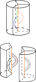
Figure 1. Stabilizing a Trisection

Stabilizing a trisection is a bit more complex than stabilizing a Heegaard splitting. However, we still obtain a new trisection $\displaystyle\mathcal{T}^{\prime}$ by modifying $\displaystyle\mathcal{T}$ in the most trivial way possible. Choose a boundary parallel, properly embedded arc $\displaystyle\alpha\subset X_{2}\cap X_{3}$ and a regular neighborhood $\displaystyle N_{1}\subset X_{2}\cap X_{3}$ of $\displaystyle\alpha.$ Choose arcs $\displaystyle\beta,\gamma$ and their neighborhoods $\displaystyle N_{2}\subset X_{1}\cap X_{3}$ and $\displaystyle N_{3}\subset X_{1}\cap X_{2}$ similarly. We define the pieces of our new trisection to be

$$\displaystyle X^{\prime}_{1}:= \displaystyle\overline{X_{1}\cup N_{1}}\setminus(N_{2}\cup N_{3})$$

$$\displaystyle X^{\prime}_{2}:= \displaystyle\overline{X_{2}\cup N_{2}}\setminus(N_{1}\cup N_{3})$$

$$\displaystyle X^{\prime}_{3}:= \displaystyle\overline{X_{3}\cup N_{3}}\setminus(N_{1}\cup N_{2})$$

Attaching the $\displaystyle 1$–handles $\displaystyle N_{i}$ to $\displaystyle X_{i}$ results in the boundary connected sum with $\displaystyle S^{1}\times B^{3}.$ However, removing the other two neighborhoods from $\displaystyle X_{i}$ do not change its topology. This is due to the fact that each curve lies in the intersection of two pieces of our trisection. This has the effect of “digging a trench” out of $\displaystyle X_{i}.$ On the other hand, each one of these neighborhoods are attached to the trisection surface which increases the genus of the trisection by three. This should be expected from the equation $\displaystyle\chi(X)=2+g-3k.$

The following theorem is the trisection analog of the Reidermeister-Singer Theorem for Heegaard splittings.

Theorem 3 (Gay-Kirby, 2012 [4]).

Every smooth, closed, connected, oriented $\displaystyle 4$–manifold admits a trisection. Moreover, any two trisections of the same $\displaystyle 4$–manifold become isotopic after a finite number of stabilizations.

As mentioned above, a relative trisection induces a structure on the bounding $\displaystyle 3$–manifold known as an open book decomposition. See [3] for a detailed introduction to open books.

Definition 2.

An open book decomposition of a connected $\displaystyle 3$–manifold $\displaystyle M$ is a pair $\displaystyle(B,\pi)$ such that $\displaystyle B$ is a link in $\displaystyle M$ called the binding and $\displaystyle\pi:M\setminus B\rightarrow S^{1}$ is a fibration such that the closure of the fibers $\displaystyle\overline{\pi^{-1}(t)}=\Sigma_{t},$ called pages, are genus $\displaystyle g$ surfaces with $\displaystyle\partial\Sigma_{t}=B$ for every $\displaystyle t.$

It is a well known result of Alexander that every $\displaystyle 3$–manifold admits an open book decomposition [1]. An abstract open book is a pair $\displaystyle(\Sigma,\phi)$, where $\displaystyle\Sigma$ is a surface with boundary and $\displaystyle\phi\in\textrm{\emph{Diff}}_{+}(\Sigma,\partial\Sigma).$ If we construct the mapping torus $\displaystyle\Sigma_{\phi}$, we can attach $\displaystyle S^{1}\times D^{2}$ to each boundary component so that $\displaystyle\partial(\Sigma\times\{t\})=\underset{b}{\sqcup}S^{1}\times\{t\}\in S^{1}\times\partial D^{2}$. The result is a closed $\displaystyle 3$–manifold $\displaystyle M_{\phi}$ equipped with an open book decomposition with pages $\displaystyle\Sigma$ and binding given by the cores of the solid tori. We will use both types of open books, depending on which one better suits our needs.

Open book decompositions can also be stabilized. Given an abstract open book $\displaystyle(P,\phi),$ choose a properly embedded arc $\displaystyle\alpha\subset P.$ Attach a $\displaystyle 2$–dimensional $\displaystyle 1$–handle to $\displaystyle\partial\alpha\times I\subset\partial P,$ giving a new surface $\displaystyle P^{\prime}.$ The co-core of the $\displaystyle 1$–handle together with $\displaystyle\alpha$ comprise a simple closed curve $\displaystyle\gamma\subset P^{\prime},$ which we require to have page framing $\displaystyle\mp 1.$ Define the new abstract open book $\displaystyle(P^{\prime},\tau^{\pm}_{\gamma}\circ\phi)$, where $\displaystyle\tau^{\pm}_{\gamma}$ denotes a positive/negative Dehn twist about $\displaystyle\gamma.$ This process is called a positive/negative Hopf stabilization of $\displaystyle(P,\phi).$ It is a standard result that $\displaystyle M_{\phi}\cong M_{\tau_{\gamma}\circ\phi}$. The page $\displaystyle P^{\prime}$ can also be viewed as the result of plumbing a Hopf band onto $\displaystyle P$ along $\displaystyle\alpha$.

Definition 3.

Let $\displaystyle S$ and $\displaystyle X$ be smooth, compact, connected, oriented manifolds of dimension $\displaystyle 2$ and $\displaystyle 4$ respectively. A Lefschetz fibration on $\displaystyle X$ is a map $\displaystyle f:X\rightarrow S,$ such that

1. $\displaystyle f$ has finitely many critical points $\displaystyle\Gamma=\{p_{1},\ldots,p_{n}\}\subset int(X)$ such that $\displaystyle f(p_{i})\neq f(p_{j})$ for $\displaystyle i\neq j$

2. around each critical point $\displaystyle f$ can be locally modeled by an orientation preserving chart as $\displaystyle f(u,v)=u_{1}^{2}+v_{2}^{2}.$

3. in the complement of the singular fibers, $\displaystyle f^{-1}(f(\Gamma)),$ $\displaystyle f$ is a smooth fibration with fibers $\displaystyle F$

The fibers of critical values are said to be singular and all other fibers are regular. Removing the condition that charts preserve orientation results in what is known as an achiral Lefschetz fibration.

Like relative trisections, Lefschetz fibrations over the disk with bounded fibers also induce open book decompositions on the boundary. Additionally, it is a straight forward process to obtain a relative trisection of $\displaystyle X$ from such a Lefschetz fibration. Thus, we will restrict our attention to Lefschetz fibrations over $\displaystyle D^{2}$ whose regular fibers are surfaces with boundary.

The critical points $\displaystyle p_{i}$ correspond to $\displaystyle 2$–handles attached to $\displaystyle F\times D^{2}$ along simple, closed curves $\displaystyle\gamma_{i}$ called vanishing cycles. The page framings of the $\displaystyle 2$–handles are $\displaystyle-1$ or $\displaystyle+1$, depending on whether the local models of the singularities are orientation preserving or reversing respectively. The induced open book decomposition is then given by $\displaystyle(F,\tau^{\pm}_{\gamma_{1}}\circ\cdots\tau^{\pm}_{\gamma_{n}})$.

We can obtain a new Lefschetz fibration $\displaystyle\mathcal{F}^{\prime}$ from $\displaystyle\mathcal{F}$ by attaching a $\displaystyle 4$–dimensional canceling $\displaystyle 1-2$ pair to $\displaystyle X$ as follows: Attach the $\displaystyle 1$–handle $\displaystyle h^{1}$ so that the attaching sphere lies in the binding of the open book decomposition of $\displaystyle\partial X$ induced by $\displaystyle f;$ thus attaching a $\displaystyle 2$–dimensional $\displaystyle 1$–handle to each of the fibers. The cancelling $\displaystyle 2$–handle $\displaystyle h^{2}$ is then attached to one of these fibers along an embedded curve with page framing $\displaystyle\pm 1$ which intersects the co-core of the new $\displaystyle 1$–handle exactly once. This ensures that $\displaystyle h^{2}$ corresponds to a Lefschetz singularity. This modification defines a new Lefschetz fibration $\displaystyle\mathcal{F}^{\prime}$ on $\displaystyle X$ whose pages and singular values differ from that of $\displaystyle\mathcal{F}$ as above. Moreover, the global monodromy of $\displaystyle\mathcal{F}^{\prime}$ is given by $\displaystyle\tau^{\mp 1}\circ\phi$, where $\displaystyle\phi$ is the monodromy of $\displaystyle\mathcal{F}.$ This modification induces a Hopf stabilization of the open book decomposition of $\displaystyle\partial X$ induced by $\displaystyle\mathcal{F}.$ (For more details see [5], [8].)

3. Trisecting Cobordisms

Just as in the closed case, a trisection of a $\displaystyle 4$–manifold $\displaystyle X$ with non-empty boundary is a decomposition $\displaystyle X=X_{1}\cup X_{2}\cup X_{3}$ where $\displaystyle X_{i}\cong\natural^{k}S^{1}\times B^{3}$, for some $\displaystyle k,$ such that the $\displaystyle X_{i}$’s have “nice” intersections. Before the proper definition can be stated, we will discuss the model pieces to which the $\displaystyle X_{i}$’s and their intersections will be diffeomorphic.

We begin with $\displaystyle F_{g,b},$ a connected genus $\displaystyle g$ surface with $\displaystyle b$ boundary components, and attach $\displaystyle n$ $\displaystyle 3$–dimensional $\displaystyle 2$–handles to $\displaystyle F_{g,b}\times\{1\}\subset F_{g,b}\times[0,1]$ along a collection of $\displaystyle n$ essential, disjoint, simple, closed curves. If $\displaystyle\partial X$ has $\displaystyle m$ connected components, then we require that surgery on $\displaystyle F_{g,b}$ along the curves separate $\displaystyle F_{g,b}$ into $\displaystyle m$ components, none of which are closed. Such a $\displaystyle 3$–manifold $\displaystyle C$ is called a compression body. We define our model pieces $\displaystyle Z:=C\times I\cong\natural^{k}S^{1}\times B^{3},$ where $\displaystyle k=2g+b-1-n.$

Remark 1.

In general, a compression body is a $\displaystyle 3$–manifold which is the result of attaching $\displaystyle 0$ and $\displaystyle 1$ handles to $\displaystyle\Sigma\times I,$ where $\displaystyle\Sigma$ is a compact surface, with or without boundary. In what follows we will only be dealing with compression bodies such as $\displaystyle C.$

It is sometimes convenient to consider a Morse function $\displaystyle f:C\rightarrow[0,1]$ with $\displaystyle f^{-1}(0)=F_{g,b}$ and $\displaystyle f^{-1}(1)=P,$ the “other end” of our compression body. We will denote $\displaystyle P=\underset{i=1}{\overset{m}{\sqcup}}P_{i},$ where $\displaystyle P_{i}\cong F_{p_{i},b_{i}},$ $\displaystyle\underset{i}{\Sigma}p_{i}=g-(n-(m-1))$ and $\displaystyle\underset{i}{\Sigma}b_{i}=b.$ The function $\displaystyle f$ will only have $\displaystyle n$ index–$\displaystyle 2$ critical points. Let us arrange for the first $\displaystyle n-(m-1)$ critical points to have distinct critical values such that passing through these critical levels does not increase the number of components of the level sets. Let us further arrange for the remaining $\displaystyle m-1$ critical points (which each correspond to a separating $\displaystyle 2$–handle) to have the same critical value. A schematic for this construction is given in Figure 2,where the red lines represent the critical levels of $\displaystyle f$)

$\displaystyle C\;\cong$ [r] at 10 55 $\displaystyle P_{1}$ at 18 162 $\displaystyle P_{m}$ at 188 162 $\displaystyle F_{g,b}$ [t] at 100 -2

$\displaystyle\cong\;Z$ [l] at 545 60 $\displaystyle F_{g,b}$ [t] at 440 -2 $\displaystyle]$ at 528 10 $\displaystyle 0$ at 522 -18 $\displaystyle 1$ at 555 20

$\displaystyle\cdots$ at 103 115

$\displaystyle\cdots$ at 440 116

$\displaystyle\leftarrow$

[l] at 175 82 $\displaystyle m-1$ separating [l] at 200 94 $\displaystyle 2$–handles [l] at 215 80 $\displaystyle\}$ at 182 29 non-separating [l] at 185 41 $\displaystyle 2$–handles [l] at 198 25

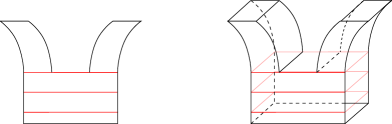
Figure 2. Constructing the Model Pieces

Note that by constructing $\displaystyle C$ upside down, it becomes immediately clear that $\displaystyle C$ is a $\displaystyle 3$–dimensional handlebody: We attach $\displaystyle n$ $\displaystyle 3$–dimensional $\displaystyle 1$–handles to $\displaystyle P\times I,$ ensuring to connect every component. Since each $\displaystyle P_{i}\times I$ is a neighborhood of a punctured surface, we have that $\displaystyle P_{i}\times I\cong\natural^{l_{i}}S^{1}\times D^{2},$ where $\displaystyle l_{i}=2p_{i}+(b_{i}-1).$ Thus, attaching $\displaystyle 1$–handles in the prescribed manner gives us

$$C\cong\natural^{k}S^{1}\times D^{2},$$

where $\displaystyle k=\underset{i}{\Sigma}l_{i}+n-(m-1)=2g+b-1-n.$ (We will regularly make use of the fact that our compression bodies are $\displaystyle 3$–dimensional handlebodies, for which it is essential that $\displaystyle F_{g,b}$ has non-empty boundary.) Thus,

$$Z\cong\natural^{k}S^{1}\times B^{3}.$$

For the intersections consider $\displaystyle\partial Z,$ which we decompose into two pieces,

$$\begin{array}[]{rl}\partial_{In}Z:=&\left(C\times\{0\}\right)\cup\left(F_{g,b}\times I\right)\cup\left(C\times\{1\}\right)\cr\partial_{Out}Z:=&\left(\partial F_{g,b}\times I\times I\right)\cup\left(P\times I\right)\\ \end{array}$$

called the inner and outer boundaries of $\displaystyle Z.$ See Figure 3. $\displaystyle\partial_{In}Z$ is the portion of $\displaystyle\partial Z$ which gets glued to the other pieces in the trisection, whereas $\displaystyle\partial_{Out}Z$ contributes to $\displaystyle\partial X.$

$\displaystyle\partial_{In}Z_{i}=$ [r] at 20 60 $\displaystyle=\partial_{Out}Z_{i}$ [l] at 533 65

$\displaystyle\cdots$ at 440 125 $\displaystyle\cdots$ at 104 108 $\displaystyle\cdots$ at 132 142

Figure 3. Decomposing $\displaystyle\partial Z$

There is a standard generalized Heegaard splitting of $\displaystyle\partial_{In}Z,$ i.e., a decomposition of a $\displaystyle 3$–manifold with boundary $\displaystyle M=C_{1}\cup C_{2},$ where $\displaystyle C_{1}\cong C_{2}$ are compression bodies which intersect along a surface with boundary. We decompose $\displaystyle\partial_{In}Z$ as

$$\partial_{In}Z=\left(C\times\{0\}\cup F_{g,b}\times[0,1/2]\right)\cup\left(F_{g,b}\times[1/2,1]\cup C\times\{1\}\right).$$

which we will denote as $\displaystyle\partial_{In}Z=Y_{0}^{+}\cup Y_{0}^{-},$ where $\displaystyle Y_{0}^{+}\cap Y_{0}^{-}\cong F_{g_{0},b}.$ We also allow for further stabilizations of this splitting (on the interior of the surface) some number of times (possibly zero) which increases the genus of the splitting. We will denote this stabilized, standard splitting as $\displaystyle\partial_{In}Z=Y^{+}\cup Y^{-},$ where $\displaystyle Y^{+}\cap Y^{-}=F_{g,b}.$ It should be noted that the stabilizations involved do not alter the $\displaystyle 4$–manifold $\displaystyle Z_{i}$ in any way, only the decomposition of the $\displaystyle 3$–manifold $\displaystyle\partial_{In}Z.$

$\displaystyle Y^{+}$ at -20 100 $\displaystyle Y^{-}$ at 440 200 $\displaystyle F_{g,b}$ [l] at 310 0

$\displaystyle\cdots$

at 105 113 $\displaystyle\cdots$ at 308 180

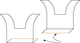
Figure 4. Decomposing $\displaystyle\partial_{In}Z$ as $\displaystyle Y^{+}\cup Y^{-}$

The “nice intersections” mentioned earlier can now be defined: $\displaystyle X_{i}\cap X_{i+1}\cong Y^{+}$ and $\displaystyle X_{i}\cap X_{i-1}\cong Y^{-}.$ Alternately phrased, $\displaystyle(X_{i}\cap X_{i+1})\cup(X_{i}\cap X_{i-1})$ is this particular generalized Heegaard splitting of $\displaystyle\partial_{In}X_{i}\cong\partial_{In}Z.$ We now give the proper definition using the above notation

Definition 4.

A relative trisection of a smooth $\displaystyle 4$–manifold with boundary $\displaystyle X$ is a decomposition $\displaystyle X=X_{1}\cup X_{2}\cup X_{3}$ such that, for some $\displaystyle Z$ with splitting $\displaystyle\partial_{In}Z=Y^{+}\cup Y^{-}$ constructed as above

1. for each $\displaystyle i$ there exists a diffeomorphism $\displaystyle\varphi_{i}:X_{i}\rightarrow Z,$

2. for each $\displaystyle i,$ we have $\displaystyle\varphi_{i}(X_{i}\cap X_{i+1})=Y^{+}$ and $\displaystyle\varphi_{i}(X_{i}\cap X_{i-1})=Y^{-}$

where indices are taken mod $\displaystyle 3$. We will sometimes denote a trisection of $\displaystyle X$ as $\displaystyle\mathcal{T}_{X},$ or $\displaystyle\mathcal{T}.$

It should be noted that the phrase “for some $\displaystyle Z$” hides many quantifiers which are necessary in defining relative trisections. We omit them in the definition because, in the case of multiple boundary components, the notation for a relative trisection can quickly become messy. Thus, we simply refer to a relative trisection as $\displaystyle\mathcal{T}$ with the understanding that the topology of $\displaystyle Z$ is determined by:

1. $\displaystyle m=|\partial X|$

2. $\displaystyle n$ - the number of $\displaystyle 2$–handles attached

3. $\displaystyle g$ - the genus of the trisection surface

4. $\displaystyle b$ - the number of boundary components of the trisection surface

5. $\displaystyle p_{i}$ - the genus of each component $\displaystyle P_{i}$ of $\displaystyle P$

As a consequence, the triple intersection $\displaystyle X_{1}\cap X_{2}\cap X_{3}=F_{g,b}$ is a surface with boundary called the trisection surface, and the outer boundaries comprise $\displaystyle\partial X.$ Let us denote $\displaystyle\partial_{Out}X_{i}=\varphi^{-1}_{i}(\partial_{Out}Z).$ Notice that $\displaystyle\partial_{Out}X_{i}=X_{i}\cap\partial X.$ The connected components of $\displaystyle\partial_{Out}X_{i}$ are given by $\displaystyle P_{i}\times I$ together with $\displaystyle\nu\partial P_{i},$ a $\displaystyle 3$–dimensional neighborhood of $\displaystyle\partial P_{i}.$ Thus, gluing the $\displaystyle X_{i}$’s to one another induces a fibration $\displaystyle\partial X\setminus\nu\partial P\rightarrow S^{1}$ with fiber $\displaystyle P.$ In other words, $\displaystyle(P,\phi)$ is an abstract open book corresponding to $\displaystyle\partial X,$ where $\displaystyle\phi$ is determined by the attaching maps $\displaystyle\{\varphi_{i}\}.$

We have thus proved the following lemma, which generalizes Gay and Kirby’s [4] result to smooth, compact $\displaystyle 4$–manifolds with an arbitrary number of boundary components.

Lemma 1.

A relative trisection of $\displaystyle X$ induces an open book decomposition of each component of $\displaystyle\partial X.$

Example 1 (Relative Trisection of $\displaystyle B^{4}$).

The simplest relative trisection is the trivial trisection of $\displaystyle B^{4}.$ Let us use the identification $\displaystyle B^{4}\cong D^{2}\times D^{2},$ where $\displaystyle D^{2}=\{re^{i\theta}\in\mathbb{C}|r\leq 1\}.$ Decompose the unit disk $\displaystyle D^{2}=D_{1}\cup D_{2}\cup D_{3},$ where $\displaystyle D_{j}=\{re^{i\theta}\in D^{2}|2\pi j/3\leq\theta\leq 2\pi(j+1)/3\}$, and let $\displaystyle p_{1}:D^{2}\times D^{2}\rightarrow D^{2}$ be the projection onto the first factor. Defining $\displaystyle X_{j}=p_{1}^{-1}(D_{j})$ yields a relative trisection of $\displaystyle B^{4}$ where

• $\displaystyle X_{i}\cong B^{4}$

• $\displaystyle X_{i}\cap X_{i+1}\cong B^{3}$

• $\displaystyle X_{1}\cap X_{2}\cap X_{3}\cong D^{2}$

Figure 5 is a $\displaystyle 3$–dimensional representation of this trisection, where the dimension of each sphere or disk is one less than the dimension of the sphere or disk it represents.

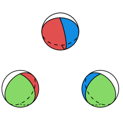
Figure 5. Trivial Trisection $\displaystyle\mathcal{B}$ of $\displaystyle B^{4}$

The colored regions on a given $\displaystyle X_{i}$ comprise $\displaystyle\partial_{In}X_{i}$ (which are modeled by $\displaystyle D^{2}$). We then take a genus–$\displaystyle 0$ generalized Heegaard splitting of $\displaystyle\partial_{In}X_{i}\cong B_{i}^{3+}\cup_{D^{2}}B_{i}^{3+}.$ Each $\displaystyle B_{i}^{3\pm}$ is colored so as to indicate where $\displaystyle X_{i}$ will glue to $\displaystyle X_{j}.$ Taking indices mod 3, we trivially glue $\displaystyle B_{i}^{3+}$ to $\displaystyle B_{i+1}^{3-}.$ Doing so yields $\displaystyle B^{4}\cong X_{1}\cup X_{2}\cup X_{3}.$ Moreover, we see that $\displaystyle\partial_{Out}X_{i}\cong B^{3}$ and our gluing gives us

$$\partial X=\bigcup_{i}\partial_{Out}X_{i}\cong S^{3}.$$

Notice that the triple intersection has boundary. In Figure 5, it is represented by the arc ($\displaystyle B^{1}$) which separates each color on the inner boundaries. As one might expect, the induced open book $\displaystyle\mathcal{B}|_{\partial B^{4}}$ is the trivial open book on $\displaystyle S^{3}.$

Example 2 (Relative Trisection of $\displaystyle S^{3}\times I$).

Let $\displaystyle\mathcal{B}_{0}$ be the trivial trisection of $\displaystyle B^{4}$ and let us take the connected sum $\displaystyle(B^{4},\mathcal{B}_{0})\#(B^{4},\mathcal{B}_{0})$ in such a way that neighborhoods of points in the trisection surfaces are identified. (For clarity, let us denote the pieces of the trisections as $\displaystyle Z_{1}\cup Z_{2}\cup Z_{3}$ and $\displaystyle Z^{\prime}_{1}\cup Z^{\prime}_{2}\cup Z^{\prime}_{3}$, where $\displaystyle Z_{i}\cong Z^{\prime}_{i}$.) The claim is that this connected sum $\displaystyle\mathcal{B}_{0}\#\mathcal{B}_{0}$ defines a relative trisection of $\displaystyle B^{4}\#B^{4}\cong S^{3}\times I.$ Let $\displaystyle B_{i}$ be a $\displaystyle 3$–ball whose boundary is decomposed as the union of two disks along their boundaries $\displaystyle\partial B_{i}=D^{+}_{i}\underset{\partial}{\cup}D^{-}_{i},$ where $\displaystyle D^{\pm}_{i}\cong D^{2}.$ By making the identifications $\displaystyle D^{+}_{i}\sim D^{-}_{i+1},$ we obtain $\displaystyle S^{3}=B_{1}\cup B_{2}\cup B_{3}$. We then extend this decomposition to $\displaystyle S^{3}\times I=(B_{1}\times I)\cup(B_{2}\times I)\cup(B_{3}\times I).$ Notice that this is not a relative trisection, as each $\displaystyle B_{i}\times I$ has not been given the structure of a model piece. In particular, it is not a thickening of a compression body from an annulus to two disjoint disks. However, each $\displaystyle B_{i}\times I$ serves as a $\displaystyle 1$–handle joining $\displaystyle Z_{i}$ and $\displaystyle Z^{\prime}_{i}$ in such a way that

$$(B_{1}\cap B_{2}\cap B_{3})\times\{0\}\subset Z_{1}\cap Z_{2}\cap Z_{3}$$

and

$$(B_{1}\cap B_{2}\cap B_{3})\times\{1\}\subset Z^{\prime}_{1}\cap Z^{\prime}_{2}\cap Z^{\prime}_{3}.$$

Thus, we have a decomposition

$$S^{3}\times I=(Z_{1}\underset{1-h}{\cup}Z^{\prime}_{1})\cup(Z_{2}\underset{1-h}{\cup}Z^{\prime}_{2})\cup(Z_{3}\underset{1-h}{\cup}Z^{\prime}_{3}).$$

Each $\displaystyle Z_{i}\underset{1-h}{\cup}Z^{\prime}_{i}$ is diffeomorphic to $\displaystyle C\times I$, where $\displaystyle C$ is the compression body obtained from attaching $\displaystyle 3$–dimensional $\displaystyle 2$–handle to $\displaystyle S^{1}\times I\times I$ along $\displaystyle S^{1}\times\{1/2\}\times\{1\}$. Moreover, we have that $\displaystyle(Z_{i}\underset{1-h}{\cup}Z^{\prime}_{i})\cap(Z_{i+1}\underset{1-h}{\cup}Z^{\prime}_{i+1})\cong B^{3}.$ Since we have taken the connected sum along the interiors, the boundary data has not been altered. Therefore, $\displaystyle\mathcal{B}_{0}\#\mathcal{B}_{0}$ is a trisection of $\displaystyle S^{3}\times I$ such that

• each piece of the trisection is $\displaystyle B^{3}$,

• the trisection surface is $\displaystyle S^{1}\times I$,

• each boundary component is endowed with the trivial open book decomposition of $\displaystyle S^{3}.$

Figure 6. Compression body $\displaystyle C\cong X_{i}\cap X_{j}$ for $\displaystyle S^{3}\times I$

The above example exhibits a bit more than a trisection of $\displaystyle S^{3}\times I.$ In fact, it shows that a connected sum of any two trisections, relative or closed, results in a trisection.

Theorem 4.

Let $\displaystyle X$ be a smooth, compact, connected $\displaystyle 4$–manifold with boundary such that each connected component of $\displaystyle\partial X$ is equipped with a fixed open book decomposition. There exists a trisection of $\displaystyle X$ which restricts to $\displaystyle\partial X$ as the given open books.

The following proof is a natural extension of the proof given by Gay and Kirby in [4] to the case of multiple boundary components.

Proof.

Let $\displaystyle(B,\phi)$ be an open book decomposition of $\displaystyle\partial X$ with page $\displaystyle P.$ If $\displaystyle\partial X$ has $\displaystyle m$ connected components, then so does $\displaystyle P.$ We will use the given boundary data to construct a Morse function $\displaystyle f:X\rightarrow I.$

Extend $\displaystyle\phi:\partial X\setminus\nu B\rightarrow S^{1}$ to the whole of $\displaystyle\partial X$, $\displaystyle\phi:\partial X\rightarrow D^{2}$ by $\displaystyle(x,z)\mapsto z$ for every $\displaystyle(x,z)\in B\times D^{2}.$ Then fix an identification of $\displaystyle D^{2}$ with $\displaystyle I\times I$ and compose $\displaystyle\phi$ with the projection onto the first factor, giving us a smooth map $\displaystyle f:\partial X\rightarrow I$ such that

1. $\displaystyle f^{-1}(0)\cong\underset{i=1}{\overset{m}{\bigsqcup}}(P_{i}\times I)\cong f^{-1}(1)$

2. $\displaystyle f^{-1}(t)\cong\underset{i=1}{\overset{m}{\bigsqcup}}\left(P_{i}\times\{0\}\cup(\partial P_{i}\times I)\cup P_{i}\times\{1\}\right)\;0<t<1.$

Extend $\displaystyle f$ to a Morse function on all of $\displaystyle X$ and consider the handle decomposition given by $\displaystyle f$. Notice that since $\displaystyle X$ is connected, if $\displaystyle m>1$ then such a function necessarily admits $\displaystyle 1$–handles. Let $\displaystyle h_{i}$ denote the number of $\displaystyle i$–handles. Without loss of generality, we can assume that the handles are ordered by index. Moreover, by adding canceling pairs we can arrange for $\displaystyle h_{1}=h_{3}.$

Let $\displaystyle\varepsilon,a\in(0,1)$ be such that $\displaystyle f^{-1}([0,\varepsilon])=f^{-1}(0)\times I$ and $\displaystyle(\varepsilon,a)$ contains all of the index $\displaystyle 1$ critical values, but no others. We then have

$$\begin{array}[]{ll}f^{-1}([0,\varepsilon])&\cong f^{-1}(0)\times I\cr&\cong(P\times I)\times I\cr&\cong\underset{i=1}{\overset{m}{\bigsqcup}}\left(\natural^{l_{i}}S^{1}\times B^{3}\right),\\ \end{array}$$

where $\displaystyle l_{i}=2p_{i}+(b_{i}-1).$ Define $\displaystyle X_{1}=f^{-1}([0,a])$. Since $\displaystyle X$ is connected, we have

$$\begin{array}[]{ll}X_{1}&\cong f^{-1}([0,\varepsilon])\cup 1\textrm{-handles}\cr&\cong\underset{i=1}{\overset{m}{\natural}}\left((\natural^{l_{i}}S^{1}\times B^{3})\natural(\natural^{h_{1}-m+1}S^{1}\times B^{3})\right)\cr&\cong\natural^{l+h_{1}-m+1}S^{1}\times B^{3},\\ \end{array}$$

where $\displaystyle l=\underset{i}{\Sigma}l_{i}.$

We will now give $\displaystyle f^{-1}(a)$ a Heegaard splitting: Define $\displaystyle N=f^{-1}(\varepsilon)$ and $\displaystyle M=\overline{\partial(f^{-1}([0,\varepsilon]))\setminus N}.$ It is not hard to see that $\displaystyle M\cong N\cong P\times I,$ and thus there is a natural generalized Heegaard splitting of $\displaystyle N\cong\left(P\times[0,1/2]\right)\cup\left(P\times[1/2,1]\right).$ Thus when we attach the $\displaystyle 1$–handles, some of which connect components to each other, we have a sort of “unbalanced decomposition” $\displaystyle\partial X_{1}=M\cup N^{\prime},$ where $\displaystyle N^{\prime}$ is diffeomorphic to

$$\left(\left(F_{p,b}\times[0,1/2]\right)\natural H_{1}\right)\bigcup\left(\left(F_{p,b}\times[1/2,1]\right)\natural H_{2}\right)$$

and $\displaystyle\#^{h_{1}-m}S^{1}\times S^{2}=H_{1}\cup H_{2}$ is the standard genus $\displaystyle h_{1}-m$ Heegaard splitting. Note that $\displaystyle N^{\prime}\cong f^{-1}(a).$ Let us denote this generalized Heegaard splitting $\displaystyle N^{\prime}=Y^{+}\cup Y^{-},$ where $\displaystyle Y^{+}$ and $\displaystyle Y^{-}$ are compression bodies from $\displaystyle F_{p+h_{1}-m+1,b}$ to $\displaystyle P$ which intersect along the surface of greater genus.

Let $\displaystyle L\subset N^{\prime}$ be the framed link which corresponds to the attaching spheres of the $\displaystyle 2$–handles given by $\displaystyle f.$ Project $\displaystyle L$ onto the splitting surface $\displaystyle F_{g,b}=Y^{+}\cap Y^{-}$ in such a way that each component of $\displaystyle L$ non-trivially contributes to the total number of self intersections, or crossings, denoted by $\displaystyle c.$ This can be done by Reidermeister $\displaystyle 1$ moves if necessary.

We first consider the special case where $\displaystyle c=h_{2}.$ Stabilizing the generalized Heegaard splitting $\displaystyle Y^{+}\cup Y^{-}$ at every crossing of $\displaystyle L$ resolves the double points by providing $\displaystyle 1$–handles whose co-cores intersect a unique link component exactly once. Additionally, every link component has such an intersection by construction. We also wish for the framings of the now embedded link $\displaystyle L$ to be consistent with the page framings. This is achieved by adding a kink via a Reidermeister $\displaystyle 1$ move and stabilizing at the new crossing. This changes the page framing by $\displaystyle\pm 1,$ which will allow us to achieve any framing through this process. Although we may have stabilized several times, we still denote $\displaystyle N^{\prime}=Y^{+}\cup Y^{-}$ with $\displaystyle Y^{+}\cap Y^{-}=F_{g,b}.$ This is pictured in Figure 7.

$\displaystyle\rightarrow$

at 132 28 R1 at 132 37

$\displaystyle\rightarrow$

at 281 28 stabilize at 280 37

Figure 7. Changing the Page Framing by $\displaystyle\pm 1$

Let us now define $\displaystyle X_{2}$ to be a collar neighborhood of $\displaystyle Y^{+}$ in the complement of $\displaystyle X_{1}$ together with the $\displaystyle 2$–handles of $\displaystyle X.$ It is important that in $\displaystyle X_{2},$ the $\displaystyle 3$–dimensional $\displaystyle 1$–handles of $\displaystyle Y^{+}$ give rise to $\displaystyle 4$–dimensional $\displaystyle 1$–handles of $\displaystyle X_{2}.$ Since we have just arranged for the attaching sphere of each $\displaystyle 2$–handle to intersect the co-cores of the $\displaystyle 1$–handles, there are $\displaystyle c=h_{2}$ canceling $\displaystyle 1-2$ pairs in $\displaystyle X_{2}.$ (We can slide $\displaystyle 1$–handles over one another to obtain a one-to-one correspondence between $\displaystyle 2$–handles and co-cores of $\displaystyle 1$–handles).

We can now verify that $\displaystyle X_{2}$ is a handlebody of the appropriate genus. First, we have that

$$\begin{array}[]{rl}Y^{+}&\cong\left(F_{p,b}\times I\right)\natural H_{1}\cr&\cong\left(\natural^{l}S^{1}\times D^{2}\right)\natural\left(\natural^{h_{1}-m+1+c}S^{1}\times D^{2}\right)\cr&\cong\natural^{l+h_{1}-m+1+c}S^{1}\times D^{2},\\ \end{array}$$

where we have taken the view that the $\displaystyle c$ stabilizations occur in $\displaystyle H_{1}\cup H_{2}.$ Finally, since we have arranged for the $\displaystyle 2$-handles to cancel $\displaystyle 1$–handles, we obtain the desired result:

$$\begin{array}[]{rl}X_{2}&\cong Y^{+}\times[0,\varepsilon]\underset{L}{\cup}2-\textrm{handles}\cr&\cong\left(\natural^{l+h_{1}-m+1+c}S^{1}\times B^{3}\right)\underset{L}{\cup}2-\textrm{handles}\cr&\cong\natural^{l+h_{1}-m+1}S^{1}\times B^{3},\\ \end{array}$$

Finally, define $\displaystyle X_{3}:=\overline{X\setminus(X_{1}\cup X_{2})}.$ Since $\displaystyle h_{1}=h_{3}$, “standing on your head” gives us $\displaystyle X_{1}\cong X_{3}.$

As for the intersections, $\displaystyle X_{1}\cap X_{2}\cong Y^{+}$ and $\displaystyle X_{1}\cap X_{3}\cong Y^{-}$ by definition. To see $\displaystyle X_{2}\cap X_{3}\cong Y^{+}$ we exploit the one-to-one correspondence between link components and a subset of the co-cores of $\displaystyle 1$–handles of $\displaystyle Y^{+}.$ Each surgery on $\displaystyle Y^{+}\times\{1\}$ defined by a link component of $\displaystyle L\subset int(Y^{+}\times\{1\})$ can be done in a unique $\displaystyle S^{1}\times D^{2}$ summand of $\displaystyle Y^{+}\times\{1\}\cong\natural S^{1}\times D^{2}.$ Such a surgery on $\displaystyle S^{1}\times D^{2}$ results in $\displaystyle S^{1}\times D^{2}$ and simply changes which curve bounds a disk. Thus, the surgery $\displaystyle 3$–manifold $\displaystyle(Y^{+}\times\{1\})_{L}$ is diffeomorphic to $\displaystyle Y^{+}.$ This completes the proof when $\displaystyle c=h_{2}.$

In the general case when $\displaystyle c>h_{2},$ we add $\displaystyle c-h_{2}$ cancelling $\displaystyle 1-2$ pairs and $\displaystyle c-h_{2}$ canceling $\displaystyle 2-3$ pairs in the original handle decomposition of $\displaystyle X$ given by $\displaystyle f.$ After said perturbation of $\displaystyle f$, we modify the pieces accordingly. (Some modifications are required to make the pieces of the trisection diffeomorphic to each other. Other modifications are needed so that the attaching spheres of the $\displaystyle 2$–handles are embedded in the trisections srurface.) We have $\displaystyle X^{\prime}_{1}=X_{1}\natural^{c-h_{2}}S^{1}\times B^{3},$ whose boundary is similarly decomposed as $\displaystyle\partial X^{\prime}_{1}=M\cup\left(N^{\prime}\#^{c-h_{2}}S^{1}\times S^{2}\right).$ Additionally, we have a new generalized Heegaard splitting of $\displaystyle N^{\prime}\#^{c-h_{2}}S^{1}\times S^{2}$

$$(Y^{+}\#\mathcal{H}_{1})\cup(Y^{-}\#\mathcal{H}_{2}),$$

where $\displaystyle\mathcal{H}_{1}\cup\mathcal{H}_{2}$ is the standard genus $\displaystyle c-h_{2}$ Heegaard splitting of $\displaystyle\#^{c-h_{2}}S^{1}\times S^{2}.$ That is, we have stabilized $\displaystyle Y^{+}\cup Y^{-}$ $\displaystyle c-h_{2}$ times, once for each newly added $\displaystyle 1$–handle. The new generalized Heegaard surface $\displaystyle F$ is of genus $\displaystyle p+h_{1}-m+c-h_{2}$ and has $\displaystyle b$ boundary components. Moreover, the original link $\displaystyle L$ projects onto $\displaystyle F$ as it did before. However, we now have an additional $\displaystyle 2(c-h_{2})$ link components corresponding to the newly added $\displaystyle 2$–handles. The half which correspond to the $\displaystyle 1-2$ pair necessarily have the canceling intersection property discussed above. The half corresponding to the $\displaystyle 2-3$ pairs project onto to $\displaystyle F$ as a $\displaystyle 0$ framed unlink which bounds disks in $\displaystyle F.$ Stabilizing $\displaystyle Y^{+}\underset{F}{\cup}Y^{-}$ for the last time(s) near each unknot allow us to slide the links into canceling position with the new $\displaystyle S^{1}\times S^{1}$ summands of $\displaystyle F.$ ∎

4. The Gluing Theorem

We now restate the gluing theorem.

Theorem 5.

Let $\displaystyle X$ and $\displaystyle W$ be smooth, compact, connected oriented $\displaystyle 4$–manifolds with non-empty boundary equipped with relative trisections $\displaystyle\mathcal{T}_{X}$ and $\displaystyle\mathcal{T}_{W}$ respectively. Let $\displaystyle B_{X}\subset\partial X$ be any collection of boundary components of $\displaystyle X$ and $\displaystyle f:B_{X}\hookrightarrow\partial W$ an injective, smooth map which respects the induced open book decompositions $\displaystyle\mathcal{T}_{X}|_{B_{X}}$ and $\displaystyle\mathcal{T}_{W}|_{f(B_{Z})}.$ Then $\displaystyle f$ induces a trisection $\displaystyle\mathcal{T}=\mathcal{T}_{X}\underset{f}{\cup}\mathcal{T}_{W}$ on $\displaystyle X\underset{f}{\cup}W.$

Note that if $\displaystyle B_{X}=\partial X=f^{-1}(\partial W)$, then the induced trisection is of a closed $\displaystyle 4$–manifold. Otherwise, we have a relative trisection of a $\displaystyle 4$–manifold with boundary. Schematics for the two possible gluings are given in Figure 8. Note that the schematic on the right depicts the gluing of only one boundary component from each manifold, but should be thought of as “not all components get glued.”

$\displaystyle\leftrightarrow$

at 18 174 $\displaystyle\cdots$ at 100 105

$\displaystyle\leftrightarrow$

at 182 174 $\displaystyle\cdots$ at 98 232

$\displaystyle\leftrightarrow$

at 509 174 $\displaystyle\cdots$ at 594 108 $\displaystyle\cdots$ at 434 238

$\displaystyle Q_{1}$

at -15 205 $\displaystyle P_{1}$ at -15 143 $\displaystyle P_{m}$ at 225 143 $\displaystyle Q_{m}$ at 225 205

$\displaystyle Q_{i}$

at 564 205 $\displaystyle P_{i}$ at 464 143

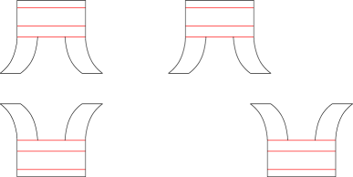
Figure 8. Gluing Relative Trisections

Proof.

Let $\displaystyle P=\underset{j=1}{\overset{m}{\sqcup}}P_{j}$ and $\displaystyle Q=\underset{j=1}{\overset{\mu}{\sqcup}}Q_{j}$ be the pages of the open books induced by $\displaystyle\mathcal{T}_{X}$ and $\displaystyle\mathcal{T}_{W}$ respectively, where $\displaystyle P_{j}\cong F_{p_{j},b_{j}}$ and $\displaystyle Q_{j}\cong F_{q_{j},d_{j}}$ for each $\displaystyle j.$ Additionally, let $\displaystyle C$ and $\displaystyle B$ denote the compression bodies which give us the $\displaystyle X_{i}$’s and $\displaystyle W_{i}$’s (i.e., $\displaystyle C\times I\cong X_{i}$ and $\displaystyle B\times I\cong W_{i}$). Let $\displaystyle n$ and $\displaystyle\eta$ denote the number of $\displaystyle 3$–dimensional $\displaystyle 1$–handles in the constructions of $\displaystyle C$ and $\displaystyle B$ respectively.

We begin with the case $\displaystyle D=\partial X\cong\partial W$ (and thus $\displaystyle m=\mu$). Our gluing is defined in the natural way, by attaching $\displaystyle\partial_{Out}X_{i}$ to $\displaystyle\partial_{Out}W_{i}$ via $\displaystyle f.$ Our new pieces are given by

$$Z_{i}:=X_{i}\underset{f}{\cup}W_{i}\;,$$

where $\displaystyle f(x)=x$ for all $\displaystyle x\in\partial_{Out}X_{i}.$ We wish to show that $\displaystyle Z_{i}$ is a $\displaystyle 4$–dimensional handlebody, and that $\displaystyle Z_{i}\cap Z_{i+1}$ and $\displaystyle Z_{i}\cap Z_{i-1}$ are $\displaystyle 3$–dimensional handlebodies. Since $\displaystyle X_{i}$ and $\displaystyle W_{i}$ are thickened compression bodies, we will reduce these to $\displaystyle 3$–dimensional arguments.

To see $\displaystyle X_{i}\cap W_{i}$ is a handlebody, we require the following simple fact:

Lemma 2.

Define the quotient space $\displaystyle M=F_{g,b}\times I/(x,t)=(x,1-t)$ for every $\displaystyle x\in\partial F_{g,b}$ and every $\displaystyle t\in I.$ $\displaystyle M$ is diffeomorphic to $\displaystyle F_{g,b}\times I.$

The main idea of the proof lies in Figure 9. We leave the details to the reader.

$\displaystyle F_{g,b}\times I$ [l] at 368 419 $\displaystyle\overset{\textit{fold}}{\longrightarrow}$ at 189 234 $\displaystyle M$ at 342 72

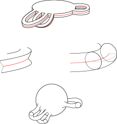
Figure 9. Proof of Lemma 2

Lemma 2 gives us $\displaystyle(P_{j}\times I)\underset{f}{\cup}(Q_{j}\times I)\cong\natural^{l_{j}}S^{1}\times D^{2}.$ We will finish constructing $\displaystyle A:=C\cup B/\sim$ by attaching the $\displaystyle 1$–handles of $\displaystyle B$ and $\displaystyle C$ to $\displaystyle(P_{j}\times I)\underset{f}{\cup}(Q_{j}\times I)$. Since the $\displaystyle 1$–handles in the construction of $\displaystyle B$ and $\displaystyle C$ are attached along the interior of level sets, the gluing and the attachment of the $\displaystyle 1$–handles can be done independently. The $\displaystyle m-1$ $\displaystyle 1$–handles coming from $\displaystyle C$ connect the $\displaystyle\natural^{l_{j}}S^{1}\times D^{2}$ to one another, yielding $\displaystyle\natural^{l}S^{1}\times D^{2}.$ The $\displaystyle m-1$ $\displaystyle 1$–handles coming from $\displaystyle B$ (which connected the $\displaystyle Q_{i}$’s in $\displaystyle B$) now increase the genus of the handlebody, leaving us with $\displaystyle\natural^{l+m-1}S^{1}\times D^{2}.$ We then proceed to attach the remaining $\displaystyle n-(m-1)$ $\displaystyle 1$–handles from $\displaystyle C$ and the remaining $\displaystyle\eta-(m-1)$ $\displaystyle 1$–handles from $\displaystyle B$. Thus, $\displaystyle A\cong\natural^{k}S^{1}\times D^{2}$, where $\displaystyle k=l+n+\eta-(m-1).$ By definition of our gluing, we have $\displaystyle A=\partial_{In}X_{i}\cup\partial_{In}W_{i}/\sim.$ Thus, $\displaystyle A=Z_{i}\cap Z_{j}$ is a $\displaystyle 3$–dimensional handlebody of genus $\displaystyle k=l+n-(m-1)+\eta-(\mu-1).$ Noting that $\displaystyle Z_{i}=A\times I$ gives us the desired result.

The more difficult case is when we wish to result in a relative trisection. For simplicity, we will prove this case when gluing $\displaystyle X$ and $\displaystyle W$ along a single boundary component given by a map which takes $\displaystyle P_{1}$ to $\displaystyle Q_{1}$ as in the right side of Figure 8. The argument easily generalizes to multiple boundary components.

Let us view $\displaystyle B$ and $\displaystyle C$ as being constructed in reverse as mentioned in the previous section. Again, the fact that the $\displaystyle 1$–handles in these constructions are attached to the interiors of $\displaystyle P$ and $\displaystyle Q$ allows us to glue $\displaystyle P_{1}\times I$ to $\displaystyle Q_{1}\times I$ before connecting components of the compression bodies. In other words, if we denote $\displaystyle M=(P_{1}\times I\underset{f}{\cup}Q_{1}\times I),$ then $\displaystyle A=C\cup B/\sim$ can be constructed by attaching $\displaystyle 1$–handles to

$$\left(\underset{i=2}{\overset{m}{\bigsqcup}}(P_{i}\times I)\right)\sqcup M\sqcup\left(\underset{i=2}{\overset{\mu}{\bigsqcup}}(Q_{i}\times I)\right).$$

Lemma 2 again gives us $\displaystyle M\cong\natural^{l_{1}}S^{1}\times D^{2}$ which can be constructed by attaching $\displaystyle l_{1}$ $\displaystyle 3$–dimensional $\displaystyle 1$–handles to $\displaystyle B^{3}.$ Thus $\displaystyle A$ can be constructed as follows: Attach $\displaystyle m-2$ $\displaystyle 1$–handles to $\displaystyle P\times I$ and $\displaystyle\mu-2$ $\displaystyle 1$–handles to $\displaystyle Q\times I$ so that each are connected. We then attach these components to $\displaystyle B^{3}$ (the $\displaystyle 0$-handle of M). Note that these two $\displaystyle 1$–handles giving us a connected manifold are the $\displaystyle 1$–handles which connect $\displaystyle P_{1}\times I$ and $\displaystyle Q_{1}\times I$ to the remaining thickened pages in $\displaystyle P\times I$ and $\displaystyle Q\times I$ respectively and do not increase the genus. To complete the construction, we attach $\displaystyle l_{1}$ $\displaystyle 1$–handles, coming from the construction of $\displaystyle M.$ This, gives us a compression body $\displaystyle A$ whose “smaller genus” end (pages of open book) is $\displaystyle\underset{j=2}{\overset{m}{\cup}}P_{j}\cup\underset{j=2}{\overset{\mu}{\cup}}Q_{j}$ and “larger genus” end is a surface of genus

$$\displaystyle\sum_{j=2}^{m}p_{j}+\sum_{j=2}^{\mu}q_{j}+(n-m+1)+(\eta-\mu+1)+\left(2p_{1}+b_{1}-1\right)$$ (4.1)

with $\displaystyle(b-b_{1})+(d-d_{1})$ boundary components.

Although the new trisection genus given by (4.1) is quite involved, the idea behind the calculation is quite simple. If $\displaystyle\mathcal{T}_{X}$ and $\displaystyle\mathcal{T}_{W}$ have relative trisection surfaces $\displaystyle F_{X}$ and $\displaystyle F_{W}$ respictively, we obtain the new trisection surface $\displaystyle F_{Z}$ by identifying the boundaries of $\displaystyle F_{X}$ and $\displaystyle F_{W}$ corresponding to the open books $\displaystyle(P_{1},\phi_{1})$ and $\displaystyle(Q_{1},\psi_{1})$ as prescribed by $\displaystyle f$.

When gluing trisections together along $\displaystyle s>1$ boundary components, we simply modify our calculation of the genus of $\displaystyle A$ to account for the fact that $\displaystyle s-1$ of the $\displaystyle 1$–handles coming from $\displaystyle B$ now increase the number of $\displaystyle S^{1}\times D^{2}$ summands. In general, we have $\displaystyle k=\underset{i=1}{\overset{s}{\Sigma}}l_{j_{i}}+n-(m-1)+\eta-(\mu-1)+(s-1).$ ∎

5. Relative Stabilizations

In this section we describe a stabilization of a relative trisections which is significantly different than that given by Gay and Kirby in that it changes the boundary data of a single boundary component and increases the trisection genus by either one or two. The effect such a relative stabilization has on the open book decomposition of the chosen boundary component of $\displaystyle\partial X$ is a Hopf stabilization; both positive and negative stabilizations can be achieved.

Given a relative trisection $\displaystyle\mathcal{T}$ of $\displaystyle X$, consider a corresponding function $\displaystyle f:X\rightarrow D^{2}$ as constructed in Theorem 4 (without identifying $\displaystyle D^{2}$ with $\displaystyle I\times I$ and projecting onto the first factor). We begin by introducing a Lefschetz singularity as in Section 2. In the case of multiple boundary components, we must choose the boundary component to which we attach the one handle, taking care that the attaching sphere of the canceling $\displaystyle 1$–handle is contained in a single boundary component $\displaystyle M_{i}\subset\partial X$ with open book $\displaystyle(P_{i},\phi_{i}).$ (Otherwise, we would be changing our $\displaystyle 4$–manifold by connecting boundary components.) We attach the $\displaystyle 2$–handle just as before, in the neighborhood of a regular value $\displaystyle y_{0}$, creating a singularity locally modeled by $\displaystyle(u,v)\mapsto u^{2}+v^{2}.$ The left half of Figure 11 shows a neighborhood of the singularity and a neighborhood of the vanishing cycle.

Remark 2.

Notice that the attaching spheres of the $\displaystyle 1$–handle can be attached to the same binding component or to different binding components. We discuss this difference below.

Let $\displaystyle Z_{f}\subset D^{2}$ denote the original critical values of $\displaystyle f$ before introducing the canceling pair. This is a codimension $\displaystyle 1$ set which is given by indefinite folds with finitely many cusps and crossings. We wish to show that we can “move $\displaystyle x_{0}$ past” all but finitely many points of $\displaystyle Z_{g}.$ That is, choosing a different regular fiber at which to attach the singular $\displaystyle 2$–handle yields an isotopic function on $\displaystyle X.$ Without loss of generality, assume $\displaystyle 0\notin Z_{f}$ and that $\displaystyle f^{-1}(0)$ is a fiber whose genus is maximal amongst regular fibers (i.e., $\displaystyle f^{-1}(0)\cong F_{g,b}$ is the trisection surface of genus $\displaystyle g$ with $\displaystyle b$ boundary components).

Let $\displaystyle\gamma:[0,1]\rightarrow D^{2}$ be a smoothly embedded path from $\displaystyle\gamma({\varepsilon})=\vec{0}$ to $\displaystyle\gamma(1-\varepsilon)=y_{0}$ such that:

• $\displaystyle\gamma$ intersects $\displaystyle Z_{f}$ at points $\displaystyle p_{1},\ldots,p_{n}\in D^{2},$ none of which are cusps or crossings of $\displaystyle Z_{f},$

• if we denote $\displaystyle p_{i}=\gamma(t_{i}),$ then $\displaystyle t_{i}<t_{i+1}$ for every $\displaystyle i,$

• the genus of the bounded fiber $\displaystyle f^{-1}(\gamma(t_{i}-\varepsilon))$ is one less than that of $\displaystyle f^{-1}(\gamma(t_{i}+\varepsilon).$

This gives us a path as in Figure 10. (The conditions above are simply to ensure that $\displaystyle\gamma$ is a path which does not intersect the same folds of $\displaystyle Z_{f}$ more than once.) Let $\displaystyle M_{\gamma}=f^{-1}(\gamma),$ then $\displaystyle\gamma^{-1}\circ f|_{M_{\gamma}}:M_{\gamma}\rightarrow[0,1]$ is a Morse function such that each $\displaystyle f^{-1}(p_{i})$ and $\displaystyle f^{-1}(y_{0})$ are index–$\displaystyle 2$ critical points. It is a standard result in Morse theory that critical points of the same index can be reordered. That is, we can modify $\displaystyle f$ so that the index–$\displaystyle 2$ critical point corresponding to the newly created Lefschetz singularity is attached to the fiber $\displaystyle f^{-1}(0).$ Finally, since it was arranged that $\displaystyle\gamma$ missed the cusps and crossings of $\displaystyle Z_{f},$ we can extend the above construction to a neighborhood $\displaystyle N\subset D^{2}$ of $\displaystyle\gamma,$ which gives a perturbed map $\displaystyle f:X\rightarrow D^{2}$ with a single Lefschetz singularity with critical value $\displaystyle\vec{0}.$

$\displaystyle Z_{f}$ at 75 122 $\displaystyle\longrightarrow$ at 195 65 $\displaystyle\gamma$ at 373 92

Figure 10. Preparing a Lefschetz Singularity for Wrinkling

Let us now perturb $\displaystyle f$ in a neighborhood of $\displaystyle\vec{0}$ via

$$f_{t}(u,v)=u^{2}+v^{2}+tRe(u),$$

or in real coordinates

$$f_{t}(s,x,y,z)=(s^{2}-x^{2}+y^{2}-z^{2}+ts,2sx_{2}yz).$$

For $\displaystyle t>0$ the critical values of $\displaystyle f_{t}$ are given by

$$\Gamma_{t}:=\{(s,x,y,z)\in\mathbb{R}^{4}|x^{2}+s^{2}+\frac{st}{2}=0,\;y=z=0\},$$

which defines a triple cuspoid pictured in Figure 11. In [7], Lekili shows that for $\displaystyle y_{1},y_{2}\in D^{2}$, where $\displaystyle y_{1}$ is in the interior of the triple cuspoid and $\displaystyle y_{2}$ is in the exterior, then the genus of $\displaystyle f_{1}^{-1}(y_{1})$ is one greater than that of $\displaystyle f_{1}^{-1}(y_{2}).$ This perturbation is known as wrinkling a Lefschetz singularity. The triple cuspoid can be thought of as a Cerf graphic, where each cusp gives a canceling $\displaystyle 1$–$\displaystyle 2$ pair and crossing a fold into the bounded region corresponds to attaching a $\displaystyle 1$–handle. Lekili further shows that crossing a fold into the exterior of the cuspoid corresponds to attaching a $\displaystyle 2$–handle along a curve in the the central fiber. In Figure 11, the colors of the attaching spheres correspond to the colors of $\displaystyle l_{ij}\subset D^{2}$ so as to indicate the isotopy class of curves determined by which fold of $\displaystyle\Gamma_{t}$ each line crosses. Notice that wrinkling is a local modification which is done on the interior of $\displaystyle X$. Thus, the action of wrinkling does not modify any boundary data.

Figure 11. Wrinkling a Lefschetz Singularity

All that remains is to show that the resulting function does in fact result in a trisected $\displaystyle 4$–manifold. Let $\displaystyle l_{ij}$ denote the image under the original map $\displaystyle f$ of $\displaystyle X_{i}\cap X_{j}$ fixed as a subset of $\displaystyle D^{2}.$ Moreover, let us arrange for the image of $\displaystyle X_{1}\cap X_{2}\cap X_{3}$ to be $\displaystyle\vec{0}.$ For sufficiently small $\displaystyle t>0$, we may assume that $\displaystyle\Gamma_{t}$ is disjoint from $\displaystyle\Gamma_{f}$ and that each $\displaystyle l_{ij}$ do not intersect $\displaystyle\Gamma_{t}$ at a cusp or crossing. If we now choose an identification of $\displaystyle D^{2}$ with $\displaystyle I\times I$, we can proceed to construct a trisection $\displaystyle\mathcal{T}^{\prime}$ of $\displaystyle X$ as in Theorem 4.

Definition 5.

The above process is a stabilization of the trisection $\displaystyle\mathcal{T}$ relative to the open book $\displaystyle(P_{i},\phi_{i}).$

By construction, a relative stabilization of $\displaystyle\mathcal{T}$ induces a stabilization of the open book decomposition $\displaystyle\mathcal{T}|_{M}=(P_{i},\phi_{i}).$ (Recall that this has the effect of plumbing a Hopf band onto the pages and the monodromy gets composed with a Dehn twist along the vanishing cycle.) If the feet of the $\displaystyle 1$–handle are contained in a single binding component, then the plumbing increases the number of boundary components of the page by one and fixes the genus. If different binding components are involved, then the plumbing decreases the number of boundary components of the page by one and increases the genus by one. As mentioned before, wrinkling the Lefschetz singularity increases the genus of the central fiber by one.

Let us now summarize stabilizations of $\displaystyle\mathcal{T}_{X}$ relative to $\displaystyle(P_{i},\phi_{i}),$ resulting in a new trisection $\displaystyle\mathcal{T}^{\prime}_{X}.$

• $\displaystyle\mathcal{T}^{\prime}$ admits a decomposition of $\displaystyle X=X^{\prime}_{1}\cup X^{\prime}_{2}\cup X^{\prime}_{3},$ where $\displaystyle X^{\prime}_{i}\cong X_{i}\natural(S^{1}\times B^{3}).$

• If $\displaystyle F_{g,b}$ is the trisection surface of $\displaystyle\mathcal{T},$ then the trisection surface of $\displaystyle\mathcal{T}^{\prime}$ is either $\displaystyle F_{g+1,b+1}$ or $\displaystyle F_{g+2,b-1}.$

• The induced open book $\displaystyle\mathcal{T}^{\prime}|_{M}=(P^{\prime}_{i},\phi^{\prime}_{i})$ is a Hopf stabilization of $\displaystyle(P_{i},\phi_{i}).$

A complete uniqueness theorem for relative trisections would require a list of stabilizations which allow us to make any two trisection of a fixed $\displaystyle 4$–manifold isotopic. It is unclear as to whether or not such a list exists (see Section 6, Question 1). However, Gay and Kirby gave the following uniqueness statement:

Theorem 6 ([4]).

Any two relative trisections of $\displaystyle X$ which induce the same open books on $\displaystyle\partial X$ can be made isotopic after a finite number of interior stabilizations of both.

Now that we have relative stabilizations at our disposal, this statement can be strengthened.

Theorem 7.

If $\displaystyle\mathcal{T}_{1}$ and $\displaystyle\mathcal{T}_{2}$ are relative trisections of $\displaystyle X$ such that their induced open books on $\displaystyle\partial X$ can be made isotopic after Hopf stabilizations, then the two relative trisections can be made isotopic after a finite number of interior and relative stabilizations of each.

Proof.

By assumption, we can perform relative stabilizations of $\displaystyle\mathcal{T}_{1}$ and $\displaystyle\mathcal{T}_{2}$ so that they induce equivalent open books on $\displaystyle\partial X.$ Since relative stabilizations, in some sense, “factor through” Lefschetz singularities, we have the liberty to choose the vanishing cycles of the associated singularities, thus allowing us to ensure that the appropriate Hopf stabilizations are induced. We now call upon the uniqueness statement of Gay and Kirby to finish the proof. ∎

Notice that relative stabilizations behave well with gluings due to the induced Hopf stabilization on the open book. More precisely,

Lemma 3.

Suppose $\displaystyle\mathcal{T}_{Z}$ and $\displaystyle\mathcal{T}_{W}$ relative trisections of $\displaystyle Z$ and $\displaystyle W$ with induced open books $\displaystyle(P,\phi)$ and $\displaystyle(Q,\psi)$ respectively. Let $\displaystyle f:\underset{r=1}{\overset{n}{\bigsqcup}}M_{\phi_{i_{r}}}\rightarrow\underset{r=1}{\overset{n}{\bigsqcup}}M_{\psi_{j_{r}}}$ be an orientation reversing diffeomorphism respecting the induced open books on each boundary component, where $\displaystyle\{i_{1},\ldots,i_{n}\},\{j_{1},\ldots,j_{n}\}\subset\{1,\ldots,m\}.$ If $\displaystyle\mathcal{T}^{\prime}_{Z}$ and $\displaystyle\mathcal{T}^{\prime}_{W}$ are relative stabilizations of $\displaystyle\mathcal{T}_{Z}$ and $\displaystyle\mathcal{T}_{W}$ relative to $\displaystyle(P_{i_{1}},\phi_{i_{1}})$ and $\displaystyle(Q_{j_{1}},\psi_{j_{1}})$ respectively such that the new induced open books remain compatible, then $\displaystyle f$ can be extended so as to induce the trisection $\displaystyle\mathcal{T}^{\prime}_{Z}\underset{f}{\cup}\mathcal{T}^{\prime}_{W}$ on $\displaystyle Z\underset{f}{\cup}W.$

The proof of the lemma is straight forward and left to the reader.

6. Final Remarks

As mentioned in Section 2, we can easily obtain a relative trisection from a Lefschetz fibration over a disk with bounded fibers. To do this, wrinkle a single Lefschetz singularity, then move the remaining singularities through the indefinite folds coming from the wrinkling as in Figure 10. Repeating this process until no Lefschetz singularities remain results in a fibration whose singular values are nested triple cuspoids in $\displaystyle D^{2}.$ A diagramatic version of this process is given in [2].

Theorems 1 and 2 allow us to define a category of trisections Tri whose object are closed $\displaystyle 3$–manifolds, either connected or disconnected, equipped with an open book decomposition and whose morphisms are relatively trisected $\displaystyle 4$–manifolds up to isotopy and interior stabilizations. Associativity is granted to us by the gluing theorem and each object has an identity since any two relative trisections of $\displaystyle X$ inducing the same open book decomposition(s) on $\displaystyle\partial X$ are stably equivalent.

Question 1.

One might hope for a full uniqueness result of relative trisections which strengthens Theorem 7 by removing the condition on the induced open book decompositions. This would require a collection of operations on relative trisections such that the induced moves on the bounding $\displaystyle 3$–manifold allows us to relate any two open book decomposition. In the case that $\displaystyle\partial X$ is a rational homology sphere, relative stabilizations are sufficient since any two open books of a rational homology sphere equivalent under Hopf stabilization. However, when dealing with an arbitrary $\displaystyle 3$–manifold, Harer provided us with the double twist in [6] (which was shown to be redundant when dealing with $\displaystyle S^{3}).$ This double twist would have to be realized as being induced by a move on relative trisections. It is clear that this can be done by taking the connected sum of two trisected $\displaystyle\mathbb{C}P^{2}$ or $\displaystyle\overline{\mathbb{C}P^{2}}.$ but we can ask if it is possible to induce a double twist on $\displaystyle\partial X$ while fixing the diffeomorphism type of the $\displaystyle X$.

References

- [1] James W. Alexander. Note on Riemann spaces. Bull. Amer. Math. Soc., 26(8):370–372, 1920.
- [2] Nickolas A. Castro, David T. Gay, and Juanita Pinzón-Caicedo. Diagrams for relative trisections. arXiV:1610.06373, 2016.
- [3] John B. Etnyre. Lectures on open book decompositions and contact structures. In Floer homology, gauge theory, and low-dimensional topology, volume 5, pages 103–141. Clay Math Proc., 2006.
- [4] David T. Gay and Robion C. Kirby. Trisecting –manifolds. Geom. Top., 20:3097–3132, 2016.
- [5] Robert E. Gompf and András I. Stipsicz. -manifolds and Kirby calculus, volume 20 of Graduate Studies in Mathematics. American Mathematical Society, Providence, RI, 1999.
- [6] John Harer. How to construct all fibered knots and links. Topology, 21(3):263–280, 1982.
- [7] Yanki Lekili. Wrinkled fibrations on near-symplectic manifolds. Geom. Topol., 13(1):277–318, 2009. Appendix B by R. İnanç Baykur.
- [8] Burak Ozbagci and András I. Stipsicz. Surgery on contact 3-manifolds and Stein surfaces, volume 13 of Bolyai Society Mathematical Studies. Springer-Verlag, Berlin; János Bolyai Mathematical Society, Budapest, 2004.