NLO QCD Corrections to Off-shell $t\,\bar{t}$ and $t\,\bar{t}\,H$ at the ILC

Abstract

We discuss top-quark physics at the ILC with a focus on the full off-shell processes for $t\bar{t}$ and $t\bar{t}H$ production, including top-quark decays and also leptonic $W$ decays. A special focus is on the matching of the resummed vNRQCD threshold calculation and the fixed-order NLO QCD continuum calculation, where we present an update on the validation of the matching. All of the calculations have been performed in the Whizard event generator framework.

1 The Whizard event generator at NLO

Whizard [1, 2] is a multi-purpose event generator for both lepton and hadron colliders. At leading-order, it can compute arbitrary SM processes and supports a multitude of BSM physics (e.g. using automated interfaces [3]). For QCD processes, it uses the color-flow formalism [4]. It has its own implementation of an analytic parton shower [5]. Moreover, it can perform simulations for a broad class of processes at next-to-leading order. The modern release series (v2) has been developed to meet the demands of LHC physics analysis, while its treatment of beam-spectra and initial-state photon radiation makes it especially well suited for lepton collider physics.

The generic next-to-leading order (NLO) framework in Whizard builds upon the FKS subtraction scheme [6, 7], which partitions the phase space into regions wherein only one divergent configuration is present. This divergence is then regulated using plus-distributions. FKS subtraction synergizes with Whizard’s optimized multi-channel phase-space generator for the underlying Born kinematics, from which real kinematics are generated. It is also very well suited to the parton shower matching procedures employed, as described below. Whizard supports OpenLoops [8], GoSam [9, 10] and RECOLA [11, 12] as one-loop matrix element providers as well as for the computation of color- and spin-correlated Born matrix elements. At tree-level, they can also be used as alternatives to Whizard’s standard matrix-element generator O’Mega [2].

For event generation, Whizard can produce weighted fixed-order NLO QCD events that are written to e.g. hepmc [13] files. This allows for flexible phenomenological fixed order studies, especially in combination with Rivet’s [14] generic event analysis capabilities. Matching to parton showers is achieved with an independent implementation [15] of the Powheg matching method [16].

Apart from scattering processes, Whizard is also able to compute decay widths for $1\to N$ processes at NLO. The final-state phase space is built in the usual fashion, whereas the initial-state phase space is adapted for decays. Computing decay widths directly in Whizard allows for a consistent treatment of top and gauge boson widths in an NLO calculation.

2 The $t\,\bar{t}$ and $t\,\bar{t}\,H$ continuum at NLO QCD

The new Whizard FKS implementation has been applied to an extensive study of fully off-shell $t\,\bar{t}$ and $t\,\bar{t}\,H$ production at a lepton collider [17]. Top-quark and leptonic $W$ decays are taken into account including the full irreducible background. The (loop) matrix elements are obtained from OpenLoops, which has been applied to a lepton collider process including hexagon diagrams for the first time. Moreover, the resonance-aware modification of FKS subtraction [18] is used to treat intermediate top, Higgs and $Z$ resonances.

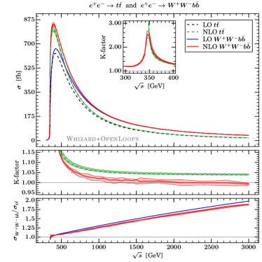
On the left-hand side of fig. 1, we show a scan of the total inclusive cross section for the on-shell process $e^{+}e^{-}\to t\,\bar{t}$ and the off-shell process $e^{+}e^{-}\to b\,W^{+}\,\bar{b}\,W^{-}$ as computed by Whizard. The most striking feature is that right above the production threshold $\sqrt{s}=2m_{t}$, both LO and NLO cross sections are strongly enhanced. Moreover, in the limit $\sqrt{s}\to 2m_{t}$ the NLO corrections to the on-shell process diverge due to non-relativistic threshold corrections, which manifest themselves as large logarithmic contributions to the virtual one-loop matrix element. In the off-shell process, the Coulomb singularity is regularized by the top-quark width, so that NLO corrections remain finite. Nevertheless, threshold corrections introduce a distinct peak in the K-factor at $\sqrt{s}=2m_{t}$, with a maximimum of about $2.5$.

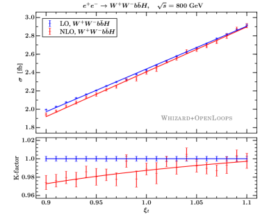
The process $e^{+}e^{-}\to t\,\bar{t}\,H$ provides a unique opportunity to measure the top Yukawa coupling $y_{t}$ [19, 20] at the per cent level. Many new physics models, such as generic 2HDMs, the MSSM or composite and Little Higgs models, predict significant deviations of $y_{t}$ from its standard model value $y_{t}^{\mathrm{SM}}=\sqrt{2}m_{t}/v$. The right-hand side of fig. 1 shows the dependence of the off-shell process on $y_{t}$, parametrized as $y_{t}=\xi_{t}y_{t}^{\mathrm{SM}}$, both at leading and next-to-leading order. The linear fit can be used to extract the parameter $\kappa$, defined via [20, 21]

$$\frac{\Delta y_{t}}{y_{t}}=\kappa\frac{\Delta\sigma}{\sigma}\;.$$ (1)

$\kappa$ contains contributions from signal, background and inteference terms. Since the $y_{t}$-dependence of the cross section on $y_{t}$ is approximately quadratic, $\kappa$ is close to $0.5$. In the above plot, we find NLO QCD corrections to $\kappa$ to be significant. They decrease $\kappa$ from the value $0.52$ at LO by about $4.6\%$ to $\kappa=0.497$ at NLO. A detailed analysis [17] reveals that these negative corrections have to originate from interference terms.

Far above the threshold, the NLO corrections are rather small for both the on-shell and the off-shell processes. For $e^{+}e^{-}\to t\,\bar{t}$, the corrections remain positive for all $\sqrt{s}$, approaching the universal massless quark pair-production factor $\alpha_{s}/\pi$ as the top mass becomes negligible. In contrast, the NLO corrections to $e^{+}e^{-}\to b\,W^{+}\,\bar{b}\,W^{-}$ decrease significantly faster for large $\sqrt{s}$, are at the per cent level for $\sqrt{s}=1500\,\mathrm{GeV}$, and come close to zero at $\sqrt{s}=3000\,\mathrm{GeV}$.

Figure 1: In the left plot, we show the total cross section for on-shell and off-shell $t\,\bar{t}$ production as a function of $\sqrt{s}$. In the lower panels, we display the K-factor for $t\,\bar{t}$ and $b\,W^{+}\,\bar{b}\,W^{-}$ in green and red, respectively, as well as the ratio of off-shell to on-shell results for LO and NLO in blue and red. In the right plot, we present the $e^{+}e^{-}\to b\,W^{+}\,\bar{b}\,W^{-}H$ LO and NLO cross sections as a function of the top Yukawa coupling modifier $\xi_{t}=y_{t}/y_{t}^{\text{SM}}$, as well as a linear fit.

3 Top-Quark threshold resummation and NLO matching

The large NLO corrections encountered in the previous section are well-known to arise from gluon exchange in the virtual correction to the top-quark production diagram. They appear as logarithms of the non-relativistic velocity $v$ and the strong coupling $\alpha_{s}$, which can be resummed. One approach for this is vNRQCD [22, 23, 24, 25], in which an effective Lagrangian for the interaction of non-relativistic heavy quark pairs is constructed. The result of the resummation can, up to NLL, be included as a simple form factor $F_{i}$ for $t\,\bar{t}$ production. Hereby, $i=\{\mathrm{LL},\mathrm{NLL}\}$ denotes the order of resummation. The vNRQCD results can be used in Whizard by embedding $F_{i}$ within a gauge-invariant description of $t\,\bar{t}$ production, as elaborated further below. In this section, we report on the recent development of the combination of the resummation with fixed-order NLO results to achieve a consistent treatment of top production at a lepton collider at all center-of-mass energies.

3.1 Setup of the calculation

3.1.1 Relativistic embedding of the form factor

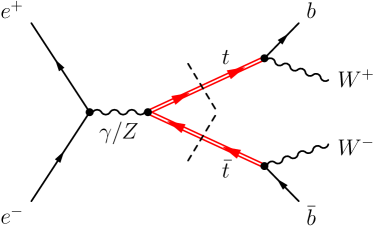
The resummed form factor is included in a gauge invariant way by factorizing the full matrix element into a production and a decay contribution,

$$\mathcal{M}=\underbrace{\left\langle{e^{+}e^{-}\vphantom{\mathcal{T}_{\mathrm{NRQCD}}{t\,\bar{t}}}\,}\right|\mathcal{T}_{\mathrm{NRQCD}}\left|{{t\,\bar{t}}\vphantom{e^{+}e^{-}\mathcal{T}_{\mathrm{NRQCD}}}}\right\rangle}_{\equiv\mathcal{M}_{\mathrm{prod}}}\left\langle{{t\,\bar{t}}\vphantom{\mathcal{T}b\,W^{+}\,\bar{b}\,W^{-}}\,}\right|\mathcal{T}\left|{b\,W^{+}\,\bar{b}\,W^{-}\vphantom{{t\,\bar{t}}\mathcal{T}}}\right\rangle,$$ (2)

where the form factor only enters the production matrix element $\mathcal{M}_{\mathrm{prod}}$. The remaining factor $\left\langle{{t\,\bar{t}}\vphantom{\mathcal{T}b\,W^{+}\,\bar{b}\,W^{-}}\,}\right|\mathcal{T}\left|{b\,W^{+}\,\bar{b}\,W^{-}\vphantom{{t\,\bar{t}}\mathcal{T}}}\right\rangle$ contains propagators and decay matrix elements for both top-quark lines. Equation 2 is represented diagrammatically in fig. 2. Specifically, we are using a double-pole approximation (DPA) [26, 27, 28, 29]. Hereby, the momenta of the top quarks and their decay products have to be projected on-shell in the matrix elements to remove gauge-dependent contributions. In the denominators of the top propagators and the phase-space Jacobians, the off-shell momenta are used. We extend the DPA also below threshold by evaluating the matrix elements with momenta at threshold. This can be seen as the closest gauge-invariant extension of the DPA that is non-zero below threshold. For comparison, we also show results in the validation that can be obtained if a gauge-dependent approach, i.e. signal diagram with off-shell momenta, is used.

Figure 2: Depiction of the factorized computation in the double pole approximation. Double lines indicate top propagators and a dashed line crossing them a factorized computation with on-shell projection.

3.1.2 Matching

The matching procedure combines the (N)LL expressions $\sigma_{\mathrm{NRQCD}}$, including the (N)LO decay, with the full fixed-order (N)LO results $\sigma_{\mathrm{FO}}$ for $b\,W^{+}\,\bar{b}\,W^{-}$ including all irreducible background processes and interferences.

By construction, the resummed result is only a valid approximation for $v\sim\alpha_{s}$. Its contribution, therefore, has to become negligible for $\left\lvert\sqrt{s}-2m_{t}\right\rvert\gg\Gamma_{t}$. This can be achieved by introducing a switch-off function $f_{s}(v)$, which is multiplied to each strong coupling constant in the resummed computation. The explicit form is arbitrary, with the minimal requirements

$$f_{s}\left(v_{\mathrm{min}}\right)=1\quad\text{and}\quad f_{s}(v=1)=0,$$ (3)

whereby the velocity $v$ takes its minimal value at threshold. Due to the presence of the width, $v_{\mathrm{min}}\sim 0.1>0$. For a realistic phenomenological description, we will switch off not too close to threshold in order to use resummed results in a region as wide as possible, but also not too far from threshold where any NRQCD loses predictivity and validity. The next cornerstone of the matching procedure is the treatment of the first order in $\alpha_{s}$. As both the resummed and the fixed-order result contain it, a naive addition of both results yields a double counting of $\mathcal{O}(\alpha_{s})$-terms. To solve this problem, we use $\sigma_{\mathrm{NRQCD}}^{\mathrm{expanded}}$, the resummed cross section expanded to $\mathcal{O}(\alpha_{s})$. Thus, the master formula for the matched cross section is

$$\sigma_{\mathrm{matched}}=\sigma_{\mathrm{FO}}\left[{\alpha_{\mathrm{H}}}\right] +\sigma_{\mathrm{NRQCD}}^{\mathrm{full}}\left[{f_{s}\,\alpha_{\mathrm{H}},\;f_{s}\,\alpha_{\mathrm{S}},\;f_{s}\,\alpha_{\mathrm{US}}}\right]{}$$

$$-\sigma_{\mathrm{NRQCD}}^{\mathrm{expanded}}\left[{f_{s}\,\alpha_{\mathrm{H}}}\right],$$ (4)

where in the full NRQCD calculation, the strong coupling has to be evaluated at hard (H), soft (S) and ultra-soft (US) scales. To remove the double counting and to ensure the NLL validity of $\sigma_{\mathrm{matched}}$, $\sigma_{\mathrm{NRQCD}}^{\mathrm{expanded}}$ has to be evaluated at the same (hard) scale as $\sigma_{\mathrm{FO}}$. Note that in eq. (3.1.2), all strong couplings in the NRQCD terms are already multiplied with $f_{s}$.

Diagramatically, eq. (3.1.2) takes the form

$$\sigma_{\mathrm{NLO+NLL}} =\sigma_{\mathrm{NLO}}+\left({\color[rgb]{0,0,1}\definecolor[named]{pgfstrokecolor}{rgb}{0,0,1}\left(\tilde{F}_{\mathrm{NLL}}-\tilde{F}^{\mathrm{exp}}_{\mathrm{NLL}}\right)}\begin{array}[]{l}\includegraphics[height=56.37271pt]{Diags/factorizedLessDetail-crop}\end{array}\right.\left\lmoustache\begin{array}[]{l}\includegraphics[height=56.37271pt]{Diags/LOfullFlipped-crop}\end{array}\right){}$$ (7)

$$+\left\lvert{\color[rgb]{0,0,1}\definecolor[named]{pgfstrokecolor}{rgb}{0,0,1}\tilde{F}_{\mathrm{NLL}}{}}\begin{array}[]{l}\includegraphics[height=56.37271pt]{Diags/factorizedLessDetail-crop}\end{array}\right\rvert^{2}{}$$ (9)

$$+\left\{{\color[rgb]{0,0,1}\definecolor[named]{pgfstrokecolor}{rgb}{0,0,1}\tilde{F}_{\mathrm{NLL}}{}}{}\hskip 13.00005pt{}\left(\begin{array}[]{l}\includegraphics[height=56.37271pt]{Diags/factorizedVirtual-crop}\end{array}+\begin{array}[]{l}\includegraphics[height=56.37271pt]{Diags/factorizedVirtualOtherLeg-crop}\end{array}\right)\right.\left\lmoustache\begin{array}[]{l}\includegraphics[height=56.37271pt]{Diags/factorizedLessDetailFlipped-crop}\end{array}{}{\color[rgb]{0,0,1}\definecolor[named]{pgfstrokecolor}{rgb}{0,0,1}\tilde{F}_{\mathrm{NLL}}{}}{}\hskip 13.00005pt{}\right\}{}$$ (13)

$$+\left\lvert{\color[rgb]{0,0,1}\definecolor[named]{pgfstrokecolor}{rgb}{0,0,1}\tilde{F}_{\mathrm{NLL}}{}}{}\begin{array}[]{l}\includegraphics[height=56.37271pt]{Diags/factorizedReal-crop}\end{array}\right\rvert^{2}+\left\lvert{\color[rgb]{0,0,1}\definecolor[named]{pgfstrokecolor}{rgb}{0,0,1}\tilde{F}_{\mathrm{NLL}}{}}{}\begin{array}[]{l}\includegraphics[height=56.37271pt]{Diags/factorizedRealOtherLeg-crop}\end{array}\right\rvert^{2},$$ (16)

with $\tilde{F}_{\mathrm{NLL}}{}=F_{\mathrm{NLL}}-1$. The first summand after $\sigma_{\mathrm{NLO}}$ is the interference term between the factorized computation, eq. 2, and the full LO amplitude, including all $2\to 4$ contributions, indicated by the gray blob. This term contains both the full form factor as well as its expansion. On the second line, we have the square of $\tilde{F}$, which is followed by its hard NLO corrections to the top decay: In the third line, we find the virtual component, indicated by the small gray blob with $\alpha_{s}$ inside. They operate only on the legs they are attached to, i.e. each blob consists of one gluon loop connecting the bottom and top quark. Finally, in the last line, there are the squared real amplitudes. Here, each gray blob represents two diagrams for gluon emission from the bottom and the top quark, respectively. Note that interference terms between the real diagrams are discarded, as they would introduce infrared divergences not cancelled by the virtual diagrams.

3.2 Implementation in Whizard

The form factor only has an analytical expression at LL, while at higher logarithmic orders, only numerical computations are possible. A dedicated tool for this is Toppik [30], which is included in the Whizard distribution.

The factorized tree-level matrix elements are calculated by modified O’Mega codes. We obtain loop matrix elements from OpenLoops. For this purpose, a dedicated matrix element library for polarized top decays is used, especially for spin correlations in top decays, which is publicly available. The one-loop decay amplitudes are then combined with the same code for the production matrix element as for tree level amplitudes.

We use the FKS setup of Whizard to evaluate eq. (7). The treatment of the fixed-order NLO cross section $\sigma_{\mathrm{NLO}}$ is identical to the previous section and ref. [17]. Thus, we can use the standard algorithm and add the result to the rest of the formula. For the remainder, slight modifications have to be made to the subtraction. They can be summed up as the following.

On-shell generation of the real-emission phase space

Like the Born matrix element, the real-emission matrix element has to be evaluated using on-shell momenta. In FKS, the phase space with an additional gluon $\Phi_{n+1}$ is constructed based on the underlying Born phase space for each possible emitter. Therefore, we already start with an on-shell projected phase space. The emission mapping then has to ensure that this property is kept. For this purpose, we use the same phase-space construction as in the resonance-aware FKS approach. There, $\Phi_{n+1}$ is constructed so that the invariant mass of the resonance associated with the emission is conserved. Fixing the invariant mass automatically ensures that an on-shell phase space stays an on-shell phase space, so that we just adopt the same mappings outlined in ref. [18].

Decay subtraction

The divergences in the factorized calculation all originate from the $t\to bWg$ matrix element. It consists of two Feynman diagrams, one in which the gluon is emitted from the top quark and another one in which it is emitted from the bottom. Divergences can only occur in emissions from particles with on-shell momenta and zero width. Therefore, in the full $b\,W^{+}\,\bar{b}\,W^{-}$ matrix element, emissions from internal top quarks do not yield divergences, as they are regulated by the width. However, in the factorized approach, the gluon emission from the top quark is a singular contribution, which needs to be subtracted. We call this additional singular region a pseudo-ISR region. This way, each FKS pair $(b,g)$ and $(\bar{b},g)$ is associated with a pseudo-ISR pair $(b,g)^{*}$ and $(\bar{b},g)^{*}$, in which the gluon radiation occurs not from the bottom, but from the top quark. This means that in the corresponding singular region, the FKS phase-space contribution $d_{ij}$ is evaluated with $p_{i}\to p_{\mathrm{top}}=p_{b}+p_{W}$.

Omission of interference terms

As outlined above, interference terms between emissions from different top-quark lines are not included in our calculation. Therefore, they also need to be dropped from the soft expressions in which mixed-emitter eikonal integrals appear.

3.3 Validation and results

Figure 3: Comparison of analytic results with the implementation in Whizard with the factorized and the signal-diagram approach for $\Delta_{m_{t}}=30\,\mathrm{GeV}$ and $\Delta_{m_{t}}=100\,\mathrm{GeV}$ using an expanded, LL or NLL form factor. The bands correspond to the envelope of the scale variations mentioned in the text.

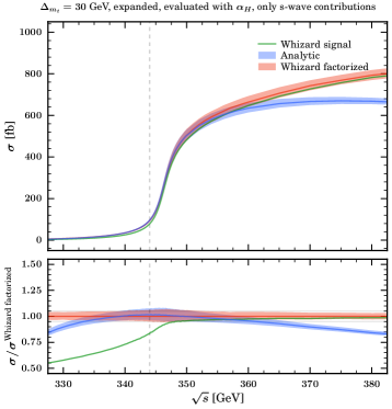
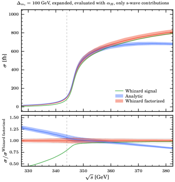
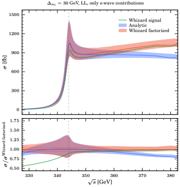
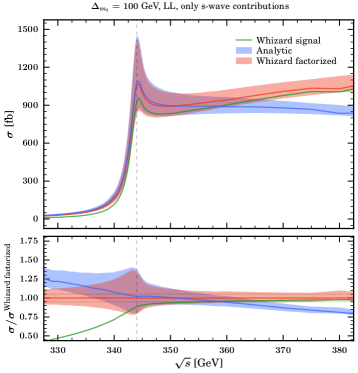
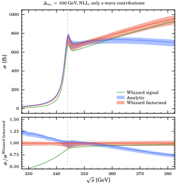
The implementation in Whizard can be checked against the analytical calculation of ref. [31]. For reliable numerical predictions, a cut $\Delta_{m_{t}}$ on the reconstructed top invariant mass is required [32], fulfilling

$$\left|\sqrt{\left(p_{W^{+}}+p_{b}\right)^{2}}-M_{t}^{1S}\right|\leq\Delta_{m_{t}}\quad\text{and}\quad\left|\sqrt{\left(p_{W^{-}}+p_{\bar{b}}\right)^{2}}-M_{t}^{1S}\right|\leq\Delta_{m_{t}}\;.$$ (17)

We stress that although this cut depends on $M_{t}^{1S}$, the invariant mass distributions will be centered around the pole mass $m_{t}$. While eq. 17 is exact in Whizard, in the analytic calculation, we implement a cut on the nonrelativistic invariant masses,

$$t_{1,2}=2m_{t}\left(E_{1,2}-\frac{\vec{p}\,^{2}}{2m_{t}}\right),$$ (18)

by requiring that

$$\left|t_{1,2}\right|\leq 2M_{t}^{1S}\Delta_{m_{t}}-\frac{3}{4}\Delta_{m_{t}}^{2}+\mathcal{O}(v^{2}).$$ (19)

Here, $E_{1,2}$ are the kinetic energies of the top and anti top quark, respectively, and $\vec{p}$ is the top quark three momentum. These different cut implementations are one source of disagreement between the Monte Carlo and the analytic results. In the threshold region, the difference should, however, be of higher order.

Figure 4: The fully matched total cross section for $e^{+}e^{-}\to b\,W^{+}\,\bar{b}\,W^{-}$ including NLO decays, the NLL form factor and the full NLO computation according to eq. 7. In addition to the three curves that are obtained for each of the three choices of the matching parameters $(v_{1},v_{2})$, we show the curve of pure fixed-order NLO and lines for NLL (red, dashed) and the matched result without switching off (black, dotted).

In fig. 3, we show $\sqrt{s}$-scans for a fixed value of $\Delta_{m_{t}}$. We have two different cut choices, a moderate, $\Delta_{m_{t}}=30\,\mathrm{GeV}$, and a loose cut, $\Delta_{m_{t}}=100\,\mathrm{GeV}$. A detailed analysis shows that the analytic computation is only reliable for moderate cuts. The plots in fig. 3, show perfect agreement between the analytic computation and Whizard for the moderate cut (${\Delta_{m_{t}}=30\,\mathrm{GeV}}$) within a window around threshold of at least $10\,\mathrm{GeV}$. For the loose cut, this range is reduced due to additional nonphysical contributions below threshold in the analytic results. For comparison, we also show the gauge-dependent results that can be obtained when embedding the form factor naively into the signal diagram, which leads to systematically lower results.

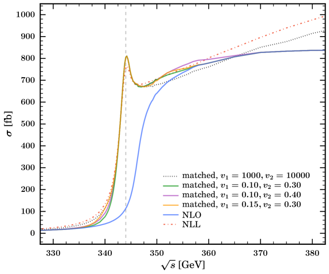
Finally, in fig. 4, we present the matched total cross section as a scan over $\sqrt{s}$ around threshold. The matched curve is similar to the pure NLL computation with LO decay around $\sqrt{s}=2M_{t}^{1S}{}$ and then smoothly approaches the fixed-order line. To estimate the error due to the arbitrary switch-off function, we have performed the computation for different values of start, $v_{1}$, and end, $v_{2}$, of the switch-off. We have experienced, furthermore, that shifting the switch-off parameters to significantly lower values, like $v_{1}=0.1,v_{2}=0.2$, cuts away too much of the threshold region and is far from the matching curve. Note that we have used $M_{t}^{1S}\sqrt{\left\lvert v\right\rvert}$ as hard scale for $\sigma_{\mathrm{FO}}$ and $\sigma_{\mathrm{NRQCD}}^{\mathrm{expanded}}$ in eq. (3.1.2) instead of the more conventional hard scale $M_{t}^{1S}$. This is the geometric mean of the hard and the soft scale and thus a more consistent choice if one aims to combine NLL and NLO results. With this choice NLO and NLL approach each other and overlap at $\sim$357\text{\,}\mathrm{GeV}$$. After this overlap, we expect the NLO to give the more reliable results for higher $\sqrt{s}$. Thus, higher values of the switch-off parameters are in principle possible but likely unnecessary. Overall, we observe fairly mild matching variation uncertainties as long as it contains the important physical regions. Finally, we want to emphasize that the matched computation, even without switch-off, realized as ($v_{1}=1000,v_{2}=10000$), does not have to be in between NLL and NLO as it is not a naive interpolation of these results but the implementation of eq. 7.

References

- [1] W. Kilian, T. Ohl and J. Reuter, Eur. Phys. J. C 71, 1742 (2011) doi:10.1140/epjc/s10052-011-1742-y [arXiv:0708.4233 [hep-ph]].
- [2] M. Moretti, T. Ohl and J. Reuter, hep-ph/0102195.
- [3] N. D. Christensen, C. Duhr, B. Fuks, J. Reuter and C. Speckner, Eur. Phys. J. C 72, 1990 (2012) doi:10.1140/epjc/s10052-012-1990-5 [arXiv:1010.3251 [hep-ph]].
- [4] W. Kilian, T. Ohl, J. Reuter and C. Speckner, JHEP 1210, 022 (2012) doi:10.1007/JHEP10(2012)022 [arXiv:1206.3700 [hep-ph]].
- [5] W. Kilian, J. Reuter, S. Schmidt and D. Wiesler, JHEP 1204, 013 (2012) doi:10.1007/JHEP04(2012)013 [arXiv:1112.1039 [hep-ph]].
- [6] S. Frixione, Z. Kunszt and A. Signer, Nucl. Phys. B 467, 399 (1996) doi:10.1016/0550-3213(96)00110-1 [hep-ph/9512328].
- [7] R. Frederix, S. Frixione, F. Maltoni and T. Stelzer, JHEP 0910, 003 (2009) doi:10.1088/1126-6708/2009/10/003 [arXiv:0908.4272 [hep-ph]].
- [8] F. Cascioli, P. Maierhofer and S. Pozzorini, Phys. Rev. Lett. 108, 111601 (2012) doi:10.1103/PhysRevLett.108.111601 [arXiv:1111.5206 [hep-ph]].
- [9] G. Cullen et al., Eur. Phys. J. C 74, no. 8, 3001 (2014) doi:10.1140/epjc/s10052-014-3001-5 [arXiv:1404.7096 [hep-ph]].
- [10] G. Cullen, N. Greiner, G. Heinrich, G. Luisoni, P. Mastrolia, G. Ossola, T. Reiter and F. Tramontano, Eur. Phys. J. C 72, 1889 (2012) doi:10.1140/epjc/s10052-012-1889-1 [arXiv:1111.2034 [hep-ph]].
- [11] S. Actis, A. Denner, L. Hofer, A. Scharf and S. Uccirati, JHEP 1304, 037 (2013) doi:10.1007/JHEP04(2013)037 [arXiv:1211.6316 [hep-ph]].
- [12] S. Actis, A. Denner, L. Hofer, J. N. Lang, A. Scharf and S. Uccirati, Comput. Phys. Commun. 214, 140 (2017) doi:10.1016/j.cpc.2017.01.004 [arXiv:1605.01090 [hep-ph]].
- [13] M. Dobbs and J. B. Hansen, Comput. Phys. Commun. 134, 41 (2001). doi:10.1016/S0010-4655(00)00189-2
- [14] A. Buckley, J. Butterworth, L. Lonnblad, D. Grellscheid, H. Hoeth, J. Monk, H. Schulz and F. Siegert, Comput. Phys. Commun. 184, 2803 (2013) doi:10.1016/j.cpc.2013.05.021 [arXiv:1003.0694 [hep-ph]].
- [15] B. Chokoufe Nejad, W. Kilian, J. Reuter and C. Weiss, PoS EPS -HEP2015, 317 (2015) [arXiv:1510.02739 [hep-ph]].
- [16] P. Nason, JHEP 0411, 040 (2004) doi:10.1088/1126-6708/2004/11/040 [hep-ph/0409146].
- [17] B. Chokoufé Nejad, W. Kilian, J. M. Lindert, S. Pozzorini, J. Reuter and C. Weiss, JHEP 1612, 075 (2016) doi:10.1007/JHEP12(2016)075 [arXiv:1609.03390 [hep-ph]].
- [18] T. Ježo and P. Nason, JHEP 1512, 065 (2015) doi:10.1007/JHEP12(2015)065 [arXiv:1509.09071 [hep-ph]].
- [19] K. Agashe et al. [Top Quark Working Group], arXiv:1311.2028 [hep-ph].
- [20] T. Price, P. Roloff, J. Strube and T. Tanabe, Eur. Phys. J. C 75, no. 7, 309 (2015) doi:10.1140/epjc/s10052-015-3532-4 [arXiv:1409.7157 [hep-ex]].
- [21] P. Roloff and J. Strube, arXiv:1307.7644 [hep-ex].
- [22] M. E. Luke, A. V. Manohar and I. Z. Rothstein, Phys. Rev. D 61, 074025 (2000) doi:10.1103/PhysRevD.61.074025 [hep-ph/9910209].
- [23] A. V. Manohar and I. W. Stewart, Phys. Rev. D 62, 014033 (2000) doi:10.1103/PhysRevD.62.014033 [hep-ph/9912226].
- [24] A. V. Manohar and I. W. Stewart, Phys. Rev. D 62, 074015 (2000) doi:10.1103/PhysRevD.62.074015 [hep-ph/0003032].
- [25] A. V. Manohar and I. W. Stewart, Phys. Rev. D 63, 054004 (2001) doi:10.1103/PhysRevD.63.054004 [hep-ph/0003107].
- [26] R. G. Stuart, Phys. Lett. B 262, 113 (1991). doi:10.1016/0370-2693(91)90653-8
- [27] A. Aeppli, G. J. van Oldenborgh and D. Wyler, Nucl. Phys. B 428, 126 (1994) doi:10.1016/0550-3213(94)90195-3 [hep-ph/9312212].
- [28] W. Beenakker, F. A. Berends and A. P. Chapovsky, Nucl. Phys. B 548, 3 (1999) doi:10.1016/S0550-3213(99)00110-8 [hep-ph/9811481].
- [29] A. Denner, S. Dittmaier, M. Roth and D. Wackeroth, Phys. Lett. B 475, 127 (2000) doi:10.1016/S0370-2693(00)00059-9 [hep-ph/9912261].
- [30] A. H. Hoang and T. Teubner, Phys. Rev. D 60, 114027 (1999) doi:10.1103/PhysRevD.60.114027 [hep-ph/9904468].
- [31] A. H. Hoang and M. Stahlhofen, JHEP 1405, 121 (2014) doi:10.1007/JHEP05(2014)121 [arXiv:1309.6323 [hep-ph]].
- [32] A. H. Hoang, C. J. Reisser and P. Ruiz-Femenia, Phys. Rev. D 82, 014005 (2010) doi:10.1103/PhysRevD.82.014005 [arXiv:1002.3223 [hep-ph]].