The Beta Flexible Weibull Distribution

Abstract

We introduce in this paper a new generalization of the flexible Weibull distribution with four parameters. This model based on the Beta generalized (BG) distribution, Eugene et al. [7], they first using the BG distribution for generating new generalizations. This new model is called the beta flexible Weibull BFW distribution. Some statistical properties such as the mode, the $r$th moment, skewness and kurtosis are derived. The moment generating function and the order statistics are obtained. Moreover, the estimations of the parameters are given by maximum likelihood method and the Fisher’s information matrix is derived. Finally, we study the advantage of the BFW distribution by an application using real data set.

 

Keywords: Beta Flexible Weibull; Beta Generalized distribution; Modified Flexible Weibull Distribution; Beta Weibull Distribution; Maximum Likelihood Method.

2010 MSC: 60E05, 62N05, 62H10

1 Introduction

In recent years appeared many generalizations which based on the Weibull (WD) distribution, Weibull[20], such as Modified Weibull (MW) distribution submitted by Lai et al. [10], and Sarhan et al. [16], generalized modified Weibull (GMW) distribution, Carrasco et al. [4]. Kumaraswamy Weibull (KW) distribution, Cordeiro et al. [5], exponentiated modified Weibull extension (EMWE) distribution, Sarhan et al. [17]. and flexible Weibull extension (FWE) distribution, introduced by Bebbington et al. [2].

We said a random variable $X$ has a flexible Weibull (FW) distribution with two parameter, if it’s cumulative distribution function (CDF) is given as follows

$$F_{FW}(x;\alpha,\beta)=1-\exp\left\{-e^{\alpha x-\frac{\beta}{x}}\right\},\quad\alpha,\beta\;\text{and}\;\;x>0.$$ (1.1)

Moreover the probability density function (PDF) corresponding Eq. (7) is given by

$$f_{FW}(x;\alpha,\beta)=(\alpha+\frac{\beta}{x^{2}})e^{\alpha x-\frac{\beta}{x}}\exp\left\{-e^{\alpha x-\frac{\beta}{x}}\right\},\quad x>0.$$ (1.2)

Some generalizations of the flexible Weibull distribution were discussed recently, such as exponentiated flexible Weibull extension (EFWE) distribution, Weibull generalized flexible Weibull extension (WG-FWE) distribution, Mustafa et al. [11], kumaraswamy flexible Weibull extension (KFWE) distribution, El Damcese et al. [6], inverse flexible Weibull extension (IFWE) distribution and exponentiated generalized flexible Weibull extension (EG-FWE) distribution, Mustafa et al. [12].

In this paper, we give a new generalization of the flexible Weibull distribution. This new generalization is called beta flexible Weibull (BFW) distribution, using class of beta generalized (BG) distribution, Eugene et al. [7]. By substituting $F(x,\varphi)$ given in Eq. (1.3) to be $F_{FW}(x,\alpha,\beta)$ given in Eq. (7).
If $F(x,\varphi)$ the baseline CDF of a random variable, then the beta generalized distribution is given by

$$F_{BG}(x;p,q,\varphi)=I_{F(x;\varphi)}(p,q)=\frac{1}{B(p,q)}\int\limits_{0}^{F(x,\varphi)}u^{p-1}(1-u)^{q-1}du,\quad p,q>0,$$ (1.3)

where $\varphi$ is the parameter vector, $I_{y}(p,q)=\frac{B_{y}(a,q)}{B(a,q)}$ is the incomplete beta function ratio, and

$$B_{y}(p,q)=\int\limits_{0}^{y}u^{p-1}(1-u)^{q-1}du.$$

The PDF of the BG distribution corresponding Eq. (1.3) is

$$f_{BG}(x;p,q,\varphi)=\frac{f(x;\varphi)}{B(p,q)}F(x;\varphi)^{p-1}\left[1-F(x;\varphi)\right]^{q-1}.$$ (1.4)

The reliability function and failure rate function of the BG distribution corresponding Eq.(1.3) are given, respectively, by the relations

$$S_{BG}(x;p,q,\varphi)=1-F_{BG}(x;p,q,\varphi)=1-I_{F(x;\varphi)}(p,q),$$ (1.5)

and

$$h_{BG}(x;p,q,\varphi)=\frac{f(x;\varphi)F(x;\varphi)^{p-1}\left[1-F(x;\varphi)\right]^{q-1}}{B(p,q)\left[1-I_{F(x;\varphi)}(p,q)\right]}.$$ (1.6)

Using expression $B(p,q)=\frac{\Gamma(p).\Gamma(q)}{\Gamma(p+q)}$, and the series representation

$$(1-u)^{q-1}=\sum_{i=0}^{q-1}\frac{(-1)^{i}\Gamma(q)}{i!\Gamma(q-i)}u^{i},\quad\text{for real non-integer}\quad|u|<1,\quad q>0,$$

the CDF of the BG distribution in Eq. (1.3) can be rewritten as follows

$$F_{BG}(x;p,q,\varphi)=\frac{\Gamma(p+q)}{\Gamma(p)}\sum_{i=0}^{q-1}\frac{(-1)^{i}\left[F(x;\varphi)\right]^{p+i}}{i!(p+i)\Gamma(q-i)},\quad p,q>0.$$ (1.7)

Recently the class of BG distribution Eq. (1.3) has been receiving considerable attention. This distribution was firstly studied by Eugene et al. [7]. Many researchers considered different forms of distribution function $F(x,\varphi)$ given in Eq. (1.3) and studied their properties. Beta normal (BN) distribution, Eugene et al. [7], beta gumbel (BG) distribution has been introduced by Nadarajah and Kotz [13], beta Weibull (BW) distribution, Famoye et al. [8], beta modified Weibull (BMW) distribution, Silva et al. [19] and beta exponential (BE) distribution, Nadarajah et al. [14].

This paper is arranged as follows, the distribution function, density function and failure rate function of the BFW distribution are defined in Section 2. Some statistical properties including, the mode, $rth$ moment, skewness and kurtosis are presented in Sections 3. The moment generating function is derived in Section 4. The order statistics is discussed in Section 5. The maximum likelihood estimation MLEs of the parameters is obtained in Section 6. Real data set are analyzed in Section 7. Moreover, we discuss the results and compare it with existing distributions. Finally, we give a conclusion in Section 8.

2 The Beta Flexible Weibull Distribution

We define the BFW($\alpha,\beta,p,q$) distribution, by substituting $F(x,\varphi)$ in Eq. (1.7) to be the distribution function $F_{FW}(x;\alpha,\beta)$ of the FWD in Eq. (7). So the CDF of the Beta Flexible Weibull distribution is

$$F_{BFW}(x;\eta)=\frac{\Gamma(p+q)}{\Gamma(p)}\sum_{i=0}^{q-1}\frac{(-1)^{i}\left[1-e^{-e^{\alpha x-\frac{\beta}{x}}}\right]^{p+i}}{i!\Gamma(q-i)(p+i)},\;\forall x>0,$$ (2.1)

where $\eta=(\alpha,\beta,p,q)$, $\alpha,\beta,p>0$ and $q>0$.
Replacing $F_{FW}(x;\alpha,\beta)$ in Eq. (7) and $f_{FW}(x;\alpha,\beta)$ in Eq. (1.2) by the $F(x,\varphi)$ and $f(x;\varphi)$ in Eq. (1.4), respectively, the PDF corresponding Eq.(2.1) can be obtained as follows

$$f_{BFW}(x;\eta)=\frac{\Gamma(p+q)}{\Gamma(p).\Gamma(q)}\left(\alpha+\frac{\beta}{x^{2}}\right)e^{\alpha x-\frac{\beta}{x}}e^{-qe^{\alpha x-\frac{\beta}{x}}}\left[1-e^{-e^{\alpha x-\frac{\beta}{x}}}\right]^{p-1}.$$ (2.2)

The reliability function $S_{BFW}(x)$ and failure rate $h_{BFW}(x)$ function of $X$ having the BFWD$(\eta)$, respectively, are given by

$$S_{BFW}(x;\eta)=1-\frac{\Gamma(p+q)}{\Gamma(p)}\sum_{i=0}^{q-1}\frac{(-1)^{i}\left[1-e^{-e^{\alpha x-\frac{\beta}{x}}}\right]^{p+i}}{i!\Gamma(q-i)(p+i)},\;\forall x>0,$$ (2.3)

and

$$h_{BFW}(x;\eta)=\frac{\frac{\Gamma(p+q)}{\Gamma(p).\Gamma(q)}\left(\alpha+\frac{\beta}{x^{2}}\right)e^{\alpha x-\frac{\beta}{x}}e^{-qe^{\alpha x-\frac{\beta}{x}}}\left[1-e^{-e^{\alpha x-\frac{\beta}{x}}}\right]^{p-1}}{1-\frac{\Gamma(p+q)}{\Gamma(p)}\sum_{i=0}^{q-1}\frac{(-1)^{i}\left[1-e^{-e^{\alpha x-\frac{\beta}{x}}}\right]^{p+i}}{i!\Gamma(q-i)(p+i)}}.$$ (2.4)

Also, the reversed failure rate $r_{BFW}(x)$ and cumulative-failure rate $H_{BFW}(x)$ functions of $X$ having the BFWD$(\eta)$, respectively, are given by

$$r_{BFW}(x;\eta)=\frac{\frac{\Gamma(p+q)}{\Gamma(p).\Gamma(q)}\left(\alpha+\frac{\beta}{x^{2}}\right)e^{\alpha x-\frac{\beta}{x}}e^{-qe^{\alpha x-\frac{\beta}{x}}}\left[1-e^{-e^{\alpha x-\frac{\beta}{x}}}\right]^{p-1}}{\frac{\Gamma(p+q)}{\Gamma(p)}\sum_{i=0}^{q-1}\frac{(-1)^{i}\left[1-e^{-e^{\alpha x-\frac{\beta}{x}}}\right]^{p+i}}{i!\Gamma(q-i)(p+i)}},$$ (2.5)

and

$$H_{BFW}(x;\eta)=\int_{0}^{x}h_{BFW}(t)dt=\int_{0}^{x}\frac{\frac{\Gamma(p+q)}{\Gamma(p).\Gamma(q)}\left(\alpha+\frac{\beta}{t^{2}}\right)e^{\alpha t-\frac{\beta}{t}}e^{-qe^{\alpha t-\frac{\beta}{t}}}\left[1-e^{-e^{\alpha t-\frac{\beta}{t}}}\right]^{p-1}}{1-\frac{\Gamma(p+q)}{\Gamma(p)}\sum_{i=0}^{q-1}\frac{(-1)^{i}\left[1-e^{-e^{\alpha t-\frac{\beta}{t}}}\right]^{p+i}}{i!\Gamma(q-i)(p+i)}}dt.$$ (2.6)

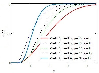
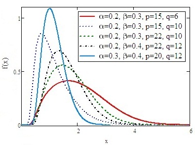
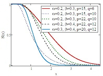
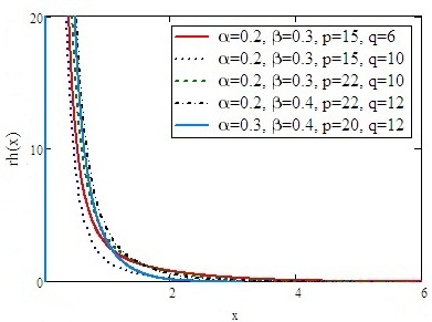
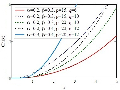
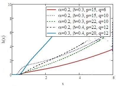
Figures 1, 2 and 3 display functions the CDF, PDF, $S_{BFW}(x)$, $h_{BFW}(x)$, $r_{BFW}(x)$ and $H_{BFW}(x)$ of the BFWD$(\eta)$ for different values of parameters.

Figure 1: Shows the CDF and PDF of the BFWD for different values of parameters

Figure 2: Shows the $S_{BFW}(x)$ and $h_{BFW}(x)$ of the BFWD for different values of parameters

Figure 3: Shows the $r_{BFW}(x)$ and $H_{BFW}(x)$ of the BFWD for different values of parameters

3 Statistical Properties

Some statistical properties for the BFWD$(\eta)$, such as the mode, the $r$th moment, skewness and kurtosis are given as follows.

3.1 The Mode of the BFWD

The mode of the BFWD$(\eta)$ can be obtained by differentiating its probability density function with respect to $x$ in Eq. (2.2) and equating it to zero.

$$f^{{}^{\prime}}(x;\eta)=0.$$

So the mode of the BFWD$(\eta)$ is solution of the following relation

$$\frac{\Gamma(p+q)}{\Gamma(p).\Gamma(q)}e^{\alpha x-\frac{\beta}{x}}e^{-qe^{\alpha x-\frac{\beta}{x}}}\left[1-e^{-e^{\alpha x-\frac{\beta}{x}}}\right]^{p-1}\times$$

$$\left\{\frac{-2\beta}{x^{3}}+(\alpha+\frac{\beta}{x^{2}})^{2}\left[1-e^{\alpha x-\frac{\beta}{x}}\left(q+\frac{(p-1)}{e^{e^{\alpha x-\frac{\beta}{x}}}-1}\right)\right]\right\}=0.$$ (3.1)

The BFWD$(\eta)$ has exactly only one peak, so this generalization is a unimodal. Figure (2) shows that Eq. (3.1) has only one solution. We can solve it numerically.

3.2 The Moments

The $rth$ moment for BFWD$(\eta)$ is given by Theorem (3.1). The gamma function with negative integer is defined by

$$\Gamma(-r)=\frac{(-1)^{r}}{r!}\left[\phi(r)-\gamma\right],$$

where $\gamma$ denote Euler’s constant which is defined as

$$\gamma=\lim_{n\rightarrow\infty}\sum_{k=1}^{n}\left(\frac{1}{k}-\ln(n)\right),\qquad\phi(r)=\sum_{i=1}^{r}\frac{1}{i},$$

see Fisher and Kilicman [9].

Theorem 3.1.

If $X$ random variable having the BFWD$(\eta)$, so the $r$th moment of $X$, is given by

$$\mu_{r}^{{}^{\prime}} = \frac{\Gamma(p+q)}{\Gamma(q)}\sum_{n=0}^{\infty}\sum_{m=0}^{\infty}\sum_{\ell=0}^{\infty}\frac{(-1)^{n+m}(q+n)^{m}(m+1)^{r+2\ell+1}\alpha^{\ell}\beta^{r+\ell+1}}{n!m!\ell!\Gamma(p-n)}\times$$ (3.2)

$$\hskip 85.35826pt\left[\alpha\Gamma(-r-\ell-1)+\frac{\Gamma(-r-\ell+1)}{(m+1)^{2}\beta}\right].$$

Proof.

The $r$th moment of the random variable $X$ with the PDF is given by

$$\mu_{r}^{{}^{\prime}}=\int\limits_{0}^{\infty}x^{r}f(x)dx.$$ (3.3)

Using PDF for the BFWD$(\eta)$ from Eq. (2.2) into Eq. (3.3) we get

$$\mu_{r}^{{}^{\prime}}=\int_{0}^{\infty}x^{r}\frac{\Gamma(p+q)}{\Gamma(p).\Gamma(q)}\left(\alpha+\frac{\beta}{x^{2}}\right)e^{\alpha x-\frac{\beta}{x}}e^{-qe^{\alpha x-\frac{\beta}{x}}}\left[1-e^{-e^{\alpha x-\frac{\beta}{x}}}\right]^{p-1}dx,$$

where the $\left[1-e^{-e^{\alpha x-\frac{\beta}{x}}}\right]^{p-1}$ can be written as

$$\left[1-e^{-e^{\alpha x-\frac{\beta}{x}}}\right]^{p-1}=\sum_{n=0}^{\infty}\frac{(-1)^{n}\Gamma(p)}{n!\Gamma(p-n)}e^{-ne^{\alpha x-\frac{\beta}{x}}},$$

then we get

$$\mu_{r}^{{}^{\prime}}=\frac{\Gamma(p+q)}{\Gamma(p).\Gamma(q)}\sum_{n=0}^{\infty}\frac{(-1)^{n}\Gamma(p)}{n!\Gamma(p-n)}\int_{0}^{\infty}x^{r}\left[\alpha+\frac{\beta}{x^{2}}\right]e^{\alpha x-\frac{\beta}{x}}e^{-(q+n)e^{\alpha x-\frac{\beta}{x}}}dx,$$

the function $e^{-(q+n)e^{\alpha x-\frac{\beta}{x}}}$, can be written as

$$e^{-(q+n)e^{\alpha x-\frac{\beta}{x}}}=\sum_{m=0}^{\infty}\frac{(-1)^{m}(q+n)^{m}}{m!}e^{m(\alpha x-\frac{\beta}{x})},$$

we obtain

$$\mu_{r}^{{}^{\prime}}=\frac{\Gamma(p+q)}{\Gamma(p).\Gamma(q)}\sum_{n=0}^{\infty}\sum_{m=0}^{\infty}\frac{(-1)^{n+m}\Gamma(p)(q+n)^{m}}{n!m!\Gamma(p-n)}\int_{0}^{\infty}x^{r}\left[\alpha+\beta x^{-2}\right]e^{(m+1)\alpha x}e^{-(m+1)\frac{\beta}{x}}dx,$$

using series expansion of $e^{(m+1)\alpha x}$,

$$e^{(m+1)\alpha x}=\sum_{\ell=0}^{\infty}\frac{(m+1)^{\ell}\alpha^{\ell}x^{\ell}}{\ell!},$$

we have

$$\mu_{r}^{{}^{\prime}} = \frac{\Gamma(p+q)}{\Gamma(p).\Gamma(q)}\sum_{n=0}^{\infty}\sum_{m=0}^{\infty}\sum_{\ell=0}^{\infty}\frac{(-1)^{n+m}\Gamma(p)(q+n)^{m}(m+1)^{\ell}\alpha^{\ell}}{n!m!\ell!\Gamma(p-n)}\times$$

$$\hskip 85.35826pt\left[\int_{0}^{\infty}\alpha x^{r+\ell}e^{-(m+1)\frac{\beta}{x}}dx+\int_{0}^{\infty}\beta x^{r+\ell-2}e^{-(m+1)\frac{\beta}{x}}dx\right],$$

where gamma function is defined by ( see Zwillinger [21]),

$$\Gamma(\nu)=x^{\nu}\int_{0}^{\infty}e^{-tx}t^{\nu-1}dt,\quad x>0.$$

Finally the $r$th moment of the BFWD$(\eta)$ can be obtained as follows

$$\mu_{r}^{{}^{\prime}} = \frac{\Gamma(p+q)}{\Gamma(q)}\sum_{n=0}^{\infty}\sum_{m=0}^{\infty}\sum_{\ell=0}^{\infty}\frac{(-1)^{n+m}(q+n)^{m}(m+1)^{r+2\ell+1}\alpha^{\ell}\beta^{r+\ell+1}}{n!m!\ell!\Gamma(p-n)}\times$$

$$\hskip 85.35826pt\left[\alpha\Gamma(-r-\ell-1)+\frac{\Gamma(-r-\ell+1)}{(m+1)^{2}\beta}\right].$$

This completes the proof.

∎

Furthermore, using the first four moments in Eq. (3.2), the measures of skewness and kurtosis of the BFWD$(\eta)$ can be expressed in the following relations, (see Bowley [3]).
The skewness of the BFWD$(\eta)$

$$Sk(X)=\frac{E(X^{3})-3\mu E(X^{2})+2\mu^{3}}{\sigma^{3}}.$$ (3.4)

The kurtosis of the BFWD$(\eta)$

$$Ku(X)=\frac{E(X^{4})-4\mu E(X^{2})+6\mu^{2}E(X^{2})-3\mu^{4}}{\sigma^{4}}.$$ (3.5)

4 The Moment Generating Function

We derive the moment generating function MGF of the BFWD$(\eta)$ by Theorem (4.1) .

Theorem 4.1.

If $X$ is a random variable having the BFWD$(\eta)$, so the moment generating function $MGF$ of $X$ is given by

$$M_{X}(t) = \frac{\Gamma(p+q)}{\Gamma(q)}\sum_{n=0}^{\infty}\sum_{m=0}^{\infty}\sum_{\ell=0}^{\infty}\sum_{r=0}^{\infty}\frac{(-1)^{n+m}(q+n)^{m}(m+1)^{r+2\ell+1}\alpha^{\ell}\beta^{r+\ell+1}t^{r}}{n!m!\ell!r!\Gamma(p-n)}\times$$ (4.1)

$$\hskip 85.35826pt\left[\alpha\Gamma(-r-\ell-1)+\frac{\Gamma(-r-\ell+1)}{(m+1)^{2}\beta}\right].$$

Proof.

The moment generating function $MGF$ of the random variable $X$ with the PDF is

$$M_{X}(t)=\int\limits_{0}^{\infty}e^{tx}f(x)dx.$$ (4.2)

Since

$$e^{tx}=\sum_{r=0}^{\infty}\frac{t^{r}x^{r}}{r!},$$

then we get

$$M_{X}(t)=\sum_{r=0}^{\infty}\frac{t^{r}}{r!}\int_{0}^{\infty}x^{r}f(x)dx.=\sum_{r=0}^{\infty}\frac{t^{r}}{r!}\mu_{r}^{{}^{\prime}}.$$ (4.3)

Using $\mu_{r}^{{}^{\prime}}$ from Eq. (3.2) into Eq. (4.3) the $MGF$ of the BFWD$(\eta)$ can be obtained as follows

$$M_{X}(t) = \frac{\Gamma(p+q)}{\Gamma(q)}\sum_{n=0}^{\infty}\sum_{m=0}^{\infty}\sum_{\ell=0}^{\infty}\sum_{r=0}^{\infty}\frac{(-1)^{n+m}(q+n)^{m}(m+1)^{r+2\ell+1}\alpha^{\ell}\beta^{r+\ell+1}t^{r}}{n!m!\ell!r!\Gamma(p-n)}\times$$

$$\hskip 85.35826pt\left[\alpha\Gamma(-r-\ell-1)+\frac{\Gamma(-r-\ell+1)}{(m+1)^{2}\beta}\right].$$

This completes the proof. ∎

5 The Order Statistics

Suppose $X_{1:n},X_{2:n},\cdots,X_{n:n}$ denote the order statistics obtained from a random sample $X_{1}$, $X_{2}$, $\cdots$, $X_{n}$ taken from a continuous population with distribution function $F_{BFW}(x;\eta)$ and density function $f_{BFW}(x;\eta)$, so the PDF of $X_{r:n}$ can be written as

$$f_{r:n}(x;\eta)=\frac{1}{B(r,n-r+1)}\left[F_{BFW}(x;\eta)\right]^{r-1}\left[1-F_{BFW}(x;\eta)\right]^{n-r}f_{BFW}(x;\eta),$$ (5.1)

where $F_{BFW}(x;\eta)$ and $f_{BFW}(x;\eta)$ are the CDF and PDF of the BFWD$(\eta)$ given by Eq. (2.1) and Eq. (2.2), respectively. Can be defined first order statistics as $X_{1:n}=\min(X_{1},X_{2},\cdots,X_{n})$, and the last order statistics as $X_{n:n}=\max(X_{1},X_{2},\cdots,X_{n})$, where $0<F_{BFW}(x;\eta)<1,$ $\forall x>0.$
The binomial expansion of $[1-F_{BFW}(x;\eta)]^{n-r}$ can be expressed as

$$\left[1-F_{BFW}(x;\eta)\right]^{n-r}=\sum_{i=0}^{n-r}\begin{pmatrix}n-r\\ i\end{pmatrix}(-1)^{i}[F_{BFW}(x;\eta)]^{i}.$$ (5.2)

Using Eq. (5.2) in Eq. (5.1), we get

$$f_{r:n}(x;\eta)=\frac{1}{B(r,n-r+1)}f_{BFW}(x;\eta)\sum_{i=0}^{n-r}\begin{pmatrix}n-r\\ i\end{pmatrix}(-1)^{i}\left[F_{BFW}(x;\eta)\right]^{i+r-1}.$$ (5.3)

Using Eq. (2.1) and Eq. (2.2) in Eq. (5.3), we obtain

$$f_{r:n}(x;\eta)=\sum_{i=0}^{n-r}\frac{(-1)^{i}n!}{i!(r-1)!(n-r-i)!}\left[F_{BFW}(x,\eta)\right]^{i+r-1}f_{BFW}(x;\eta).$$ (5.4)

Equation (5.4) shows that the $f_{r:n}(x;\eta)$ is the weighted average of the BFWD$(\eta)$ with various shape parameters.

6 Parameters Estimation

Parameters estimation of the BFWD$(\alpha,\beta,p,q)$, point and interval estimation are derived by using maximum likelihood estimation MLE method with a complete sample.

6.1 Maximum likelihood estimation

Let $x_{1},x_{2},\cdots,x_{n}$ denote a random sample of complete data from the BFWD$(\eta)$. The Likelihood function $L$ is defined as follows

$$L=\prod_{i=1}^{n}f(x_{i};\vartheta).$$ (6.1)

Using Eq.(2.2) in Eq.(6.1), we have

$$L=\prod_{i=1}^{n}\frac{\Gamma(p+q)}{\Gamma(p).\Gamma(q)}\left(\alpha+\frac{\beta}{x_{i}^{2}}\right)e^{\alpha x_{i}-\frac{\beta}{x_{i}}}e^{-qe^{\alpha x_{i}-\frac{\beta}{x_{i}}}}\left[1-e^{-e^{\alpha x_{i}-\frac{\beta}{x_{i}}}}\right]^{p-1}.$$

The log-likelihood function is

$$\mathcal{L}=n\left[\ln\left(\frac{\Gamma(p+q)}{\Gamma(p).\Gamma(q)}\right)\right]+\sum_{i=1}^{n}\ln\left(\alpha+\frac{\beta}{x_{i}^{2}}\right)+\sum_{i=1}^{n}\left(\alpha x_{i}-\frac{\beta}{x_{i}}\right)-q\sum_{i=1}^{n}e^{\alpha x_{i}-\frac{\beta}{x_{i}}}+(p-1)\sum_{i=1}^{n}\ln\left(1-e^{-e^{\alpha x_{i}-\frac{\beta}{x_{i}}}}\right).$$ (6.2)

The MLE of the parameters $\alpha,\beta,p$ and $q$ are obtained by differentiating the function $\mathcal{L}$ in Equation (6.2) with respect to $\alpha,\beta,p$ and $q$, then equating it to zero, as follows

$$\frac{\partial\mathcal{L}}{\partial\alpha} = \sum_{i=1}^{n}\frac{x_{i}^{2}}{\beta+\alpha x_{i}^{2}}+\sum_{i=1}^{n}x_{i}-q\sum_{i=1}^{n}x_{i}e^{\alpha x_{i}-\frac{\beta}{x_{i}}}+(p-1)\sum_{i=1}^{n}\frac{x_{i}e^{\alpha x_{i}-\frac{\beta}{x_{i}}}}{e^{e^{\alpha x_{i}-\frac{\beta}{x_{i}}}}-1}=0,$$ (6.3)

$$\frac{\partial\mathcal{L}}{\partial\beta} = \sum_{i=1}^{n}\frac{1}{\beta+\alpha x_{i}^{2}}-\sum_{i=1}^{n}\frac{1}{x_{i}}+q\sum_{i=1}^{n}\frac{1}{x_{i}}e^{\alpha x_{i}-\frac{\beta}{x_{i}}}-(p-1)\sum_{i=1}^{n}\frac{e^{\alpha x_{i}-\frac{\beta}{x_{i}}}}{x_{i}\left(e^{e^{\alpha x_{i}-\frac{\beta}{x_{i}}}}-1\right)}=0,$$ (6.4)

$$\frac{\partial\mathcal{L}}{\partial p} = n\psi_{p}(p+q)-n\psi(p)+\sum_{i=1}^{n}\ln\left(1-e^{-e^{\alpha x_{i}-\frac{\beta}{x_{i}}}}\right)=0,$$ (6.5)

$$\frac{\partial\mathcal{L}}{\partial q} = n\psi_{q}(p+q)-n\psi(q)-\sum_{i=1}^{n}e^{\alpha x_{i}-\frac{\beta}{x_{i}}}=0.$$ (6.6)

The MLEs can be obtained by solving the equations, (6.3)-(6.6), numerically for $\alpha,\beta,p$ and $q$ by using Mathcad or Maple software.

6.2 Asymptotic confidence bounds

The asymptotic confidence intervals can be obtained by using variance covariance matrix $I^{-1}$, since the parameters ($\alpha,\beta,p,q$) are positive and the $I^{-1}$ is inverse of the observed information matrix given by

$$\mathbf{I^{-1}} = \left(\begin{array}[]{cccc}-\frac{\partial^{2}\mathcal{L}}{\partial\alpha^{2}}&-\frac{\partial^{2}\mathcal{L}}{\partial\alpha\partial\beta}&-\frac{\partial^{2}\mathcal{L}}{\partial\alpha\partial p}&-\frac{\partial^{2}\mathcal{L}}{\partial\alpha\partial q}\\ -\frac{\partial^{2}\mathcal{L}}{\partial\beta\partial\alpha}&-\frac{\partial^{2}\mathcal{L}}{\partial\beta^{2}}&-\frac{\partial^{2}\mathcal{L}}{\partial\beta\partial p}&-\frac{\partial^{2}\mathcal{L}}{\partial\beta\partial q}\\ -\frac{\partial^{2}\mathcal{L}}{\partial p\partial\alpha}&-\frac{\partial^{2}\mathcal{L}}{\partial p\partial\beta}&-\frac{\partial^{2}\mathcal{L}}{\partial p^{2}}&-\frac{\partial^{2}\mathcal{L}}{\partial p\partial q}\\ -\frac{\partial^{2}\mathcal{L}}{\partial q\partial\alpha}&-\frac{\partial^{2}\mathcal{L}}{\partial q\partial\beta}&-\frac{\partial^{2}\mathcal{L}}{\partial q\partial p}&-\frac{\partial^{2}\mathcal{L}}{\partial q^{2}}\end{array}\right)^{-1}=\left(\begin{array}[]{cccc}var(\hat{\alpha})&cov(\hat{\alpha},\hat{\beta})&cov(\hat{\alpha},\hat{p})&cov(\hat{\alpha},\hat{q})\\ cov(\hat{\beta},\hat{\alpha})&var(\hat{\beta})&cov(\hat{\beta},\hat{p})&cov(\hat{\beta},\hat{q})\\ cov(\hat{p},\hat{\alpha})&cov(\hat{p},\hat{\beta})&var(\hat{p})&cov(\hat{p},\hat{q})\\ cov(\hat{q},\hat{\alpha})&cov(\hat{q},\hat{\beta})&cov(\hat{q},\hat{p})&var(\hat{q})\end{array}\right),$$ (6.15)

where

$$\frac{\partial^{2}\mathcal{L}}{\partial\alpha^{2}} = -\sum_{i=1}^{n}\frac{x_{i}^{4}}{\left(\beta+\alpha x_{i}^{2}\right)^{2}}-q\sum_{i=1}^{n}x_{i}^{2}e^{\alpha x_{i}-\frac{\beta}{x_{i}}}+(p-1)\sum_{i=1}^{n}x_{i}H_{i},$$ (6.17)

$$\frac{\partial^{2}\mathcal{L}}{\partial\alpha\partial\beta} = -\sum_{i=1}^{n}\frac{x_{i}^{2}}{\left(\beta+\alpha x_{i}^{2}\right)^{2}}+q\sum_{i=1}^{n}e^{\alpha x_{i}-\frac{\beta}{x_{i}}}-(p-1)\sum_{i=1}^{n}H_{i},$$ (6.18)

$$\frac{\partial^{2}\mathcal{L}}{\partial\alpha\partial p} = \sum_{i=1}^{n}\frac{x_{i}e^{\alpha x_{i}-\frac{\beta}{x_{i}}}}{\left[e^{e^{\alpha x_{i}-\frac{\beta}{x_{i}}}}-1\right]},$$ (6.19)

$$\frac{\partial^{2}\mathcal{L}}{\partial\alpha\partial q} = -\sum_{i=1}^{n}x_{i}e^{\alpha x_{i}-\frac{\beta}{x_{i}}},$$ (6.20)

$$\frac{\partial^{2}\mathcal{L}}{\partial\beta^{2}} = -\sum_{i=1}^{n}\frac{1}{\left(\beta+\alpha x_{i}^{2}\right)^{2}}-q\sum_{i=1}^{n}\frac{e^{\alpha x_{i}-\frac{\beta}{x_{i}}}}{x_{i}^{2}}+(p-1)\sum_{i=1}^{n}\frac{H_{i}}{x_{i}^{2}},$$ (6.21)

$$\frac{\partial^{2}\mathcal{L}}{\partial\beta\partial p} = -\sum_{i=1}^{n}\frac{e^{\alpha x_{i}-\frac{\beta}{x_{i}}}}{x_{i}\left[e^{e^{\alpha x_{i}-\frac{\beta}{x_{i}}}}-1\right]},$$ (6.22)

$$\frac{\partial^{2}\mathcal{L}}{\partial\beta\partial q} = \sum_{i=1}^{n}\frac{e^{\alpha x_{i}-\frac{\beta}{x_{i}}}}{x_{i}},$$ (6.23)

$$\frac{\partial^{2}\mathcal{L}}{\partial p^{2}} = n\frac{\partial^{2}}{\partial p^{2}}\ln\left[\Gamma(p+q)\right]-n\frac{\partial^{2}}{\partial p^{2}}\ln\left[\Gamma(p)\right],$$ (6.24)

$$\frac{\partial^{2}\mathcal{L}}{\partial p\partial q} = n\frac{\partial^{2}}{\partial p\partial q}\ln\left[\Gamma(p+q)\right],$$ (6.25)

$$\frac{\partial^{2}\mathcal{L}}{\partial q^{2}} = n\frac{\partial^{2}}{\partial q^{2}}\ln\left[\Gamma(p+q)\right]-n\frac{\partial^{2}}{\partial q^{2}}\ln\left[\Gamma(q)\right],$$ (6.26)

where

$$H_{i}=\frac{x_{i}e^{\alpha x_{i}-\frac{\beta}{x_{i}}}\left[e^{e^{\alpha x_{i}-\frac{\beta}{x_{i}}}}\left(1-e^{\alpha x_{i}-\frac{\beta}{x_{i}}}\right)-1\right]}{\left[e^{e^{\alpha x_{i}-\frac{\beta}{x_{i}}}}-1\right]^{2}}.$$

Moreover, the $(1-\lambda)100\%$ confidence intervals of the four parameters can be obtained by using variance matrix as follows

$$\hat{\alpha}\pm Z_{\frac{\lambda}{2}}\sqrt{var(\hat{\alpha})},\quad\hat{\beta}\pm Z_{\frac{\lambda}{2}}\sqrt{var(\hat{\beta})},\quad\hat{p}\pm Z_{\frac{\lambda}{2}}\sqrt{var(\hat{p})},\quad\hat{q}\pm Z_{\frac{\lambda}{2}}\sqrt{var(\hat{q})},$$

where $\lambda>0$, and $Z_{\frac{\lambda}{2}}$ denote the upper $(\frac{\lambda}{2})$-th percentile of standard normal distribution.

7 Application

In this Section, we will analysis a real data set using the BFWD $(\alpha,\beta,p,q)$ and compare it with the other fitted distributions such as flexible Weibull extension distribution (FWED), Weibull distribution (WD), Modified Weibull distribution (MWD), Reduced Additive Weibull distribution (RAWD) and Extended Weibull distribution (EWD) by using some criteria statistical such as K–S statistics ( Kolmogorov Smirnov), Akaike information criterion $AIC$ and Akaike Information criterion with correction $AICC$, see [1]. Moreover, we use Bayesian information criterion $BIC$, see [18].

We will use the data given by Salman et al. [15], in Table 1.

Table 1: Time between failures of secondary reactor pumps, (thousands of hours) [15]

2.160	0.746	0.402	0.954	0.491	6.560	4.992	0.347
0.150	0.358	0.101	1.359	3.465	1.060	0.614	1.921
4.082	0.199	0.605	0.273	0.070	0.062	5.320

Table 2 gives MLEs of parameters of the BFWD$(\eta)$ and the Statistics K–S. The values of $AIC$, $AICC$, $BIC$, $HQIC$ and the log-likelihood functions $\mathcal{L}$ are in Table 3.

Table 2: MLEs and K–S of parameters for secondary reactor pumps.

Model	$\hat{\alpha}$	$\hat{\beta}$	$\hat{p}$	$\hat{q}$	K–S
FWD	0.0207	2.5875	–	–	0.1342
WD	0.8077	13.9148	–	–	0.1173
MWD	0.1213	0.7924	0.0009	–	0.1188
RAWD	0.0070	1.7292	0.0452	–	0.1619
EWD	0.4189	1.0212	10.2778	–	0.1057
BFWD	0.052	0.024	35.077	20.328	0.1151

Table 3: Log-likelihood $\mathcal{L}$, $AIC$, $AICC$,$BIC$ and $HQIC$ values of models fitted.

Model	$\mathcal{L}$	-2 $\mathcal{L}$	AIC	AICC	BIC	HQIC
FWD	-83.3424	166.6848	170.6848	171.2848	172.95579	171.2559
WD	-85.4734	170.9468	174.9468	175.5468	177.21779	175.5179
MWD	-85.4677	170.9354	176.9354	178.1986	180.34188	177.7921
RAWD	-86.0728	172.1456	178.1456	179.4088	181.55208	179.0023
EWD	-86.6343	173.2686	179.2686	180.5318	182.67508	180.1253
BFWD	-30.768	61.5360	69.5360	71.7582	74.0780	70.6783

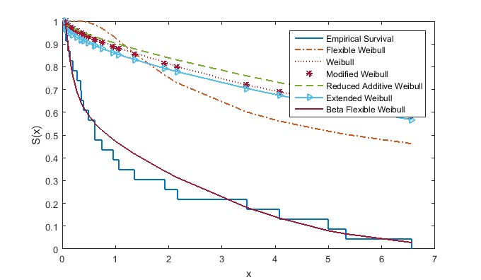
We find that the BFWD$(\eta)$ with the parameters $(\alpha,\beta,p,q)$ gives a better fit to data set than the previous generalizations of Weibull distributions such as a flexible Weibull distribution FWD, Weibull distribution WD, Modified Weibull distribution MWD, Reduced Additive Weibull distribution RAWD and Extended Weibull distribution EWD. It has the largest likelihood function $L$, and the smallest criteria values $AIC$, $AICC$, $BIC$, $HQIC$ and K–S as shown in Tables 2 and 3.

Replace the MLEs of the unknown parameters for BFWD$(\alpha,\beta,p,q)$ into Eq. (6.15), we can obtained estimation of the variance covariance matrix as follows

$$I_{0}^{-1}=\left(\begin{array}[]{cccc}2.123\times 10^{-3}&9.575\times 10^{-4}&-2.748&-1.6\\ 9.575\times 10^{-4}&5.558\times 10^{-4}&-1.415&-0.81\\ -2.748&-1.415&3.912\times 10^{3}&2.256\times 10^{3}\\ -1.6&-0.81&2.256\times 10^{3}&1.304\times 10^{3}\\ \end{array}\right).$$

The confidence intervals for approximately 95% two sided of the unknown parameters $\alpha,\beta,p$ and $q$ are $\left[0,0.142\right]$, $\left[0,0.07\right]$, $\left[0,157.671\right]$ and $\left[0,91.105\right]$, respectively.

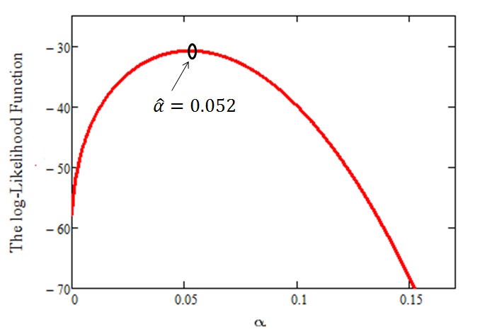
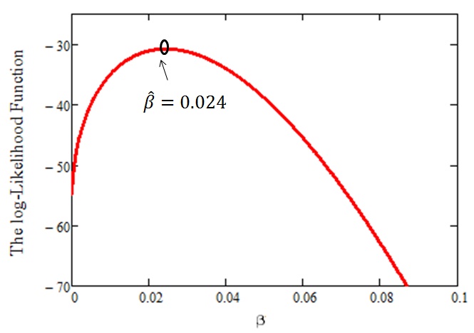
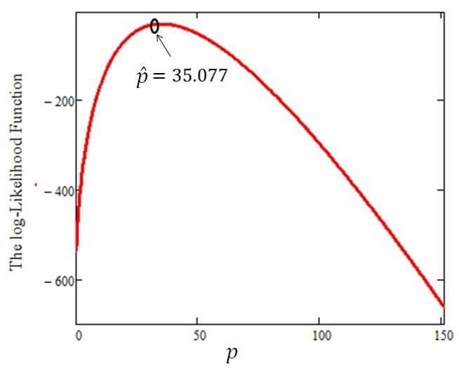
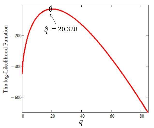
From, Figures 4 and 5 can be seen that the log-likelihood function $\mathcal{L}$ have unique solution.

Figure 4: The profile of the log-likelihood function of $\alpha,\beta$.

Figure 5: The profile of the log-likelihood function of $p$ and $q$.

Figure 6, represents the estimation for the reliability function $S(x)$, by using the Kaplan-Meier method and its fitted parametric estimations when the distribution is assumed to be FWD, WD, MWD, RAWD, EWD and BFWD are computed and plotted in the following shape.

Figure 6: Display the Kaplan-Meier estimate of the reliability function for the data.

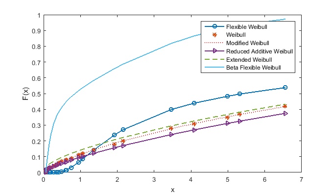
Figure 7 gives the shape of the distribution function for the FWD, WD, MWD, RAWD, EWD and BFWD after that the unknown parameters included in each distribution are replaced by their maximum likelihood estimation MLE

Figure 7: The Fitted cumulative distribution function for the data.

8 Conclusion

We studied a new generalized distribution, based on the beta generated method. This new generalization is called the beta flexible Weibull BFWD distribution . Its definition and some of statistical properties are studied. The maximum likelihood method is used for estimating parameters. The advantage of the BFWD is interpreted by an application using real data. Moreover, it is shown that the beta flexible Weibull BFWD distribution fits better than existing generalizations of the Weibull distribution.

References

• [1] H. Akaike, A new look at the statistical model identification, IEEE Transactions on Automatic Control, AC-19, 716–23, 1974.
• [2] M. S. Bebbington, C. D. Lai and R. Zitikis, A flexible Weibull extension, Reliability Engineering & System Safety, 92(6), 719–26, 2007.
• [3] A. L. Bowley, Elements of Statistics, New York: Charles Scribner’s Sons, 1920.
• [4] M. Carrasco, E. M. Ortega and G. M. Cordeiro, A generalized modified Weibull distribution for lifetime modeling, Computational Statistics and Data Analysis, 53(2), 450–62, 2008.
• [5] G. M. Cordeiro, E. M. Ortega and S. Nadarajah, The Kumaraswamy Weibull distribution with application to failure data, Journal of the Franklin Institute, 347, 1399–429, 2010.
• [6] M. A. El-Damcese, A.  Mustafa, B. S. El-Desouky and M. E. Mustafa, The Kumaraswamy Flexible Weibull Extension, International Journal of Mathematics And its Applications, 4(1-A), 1–14, 2016.
• [7] N. Eugene, C. Lee, and F. Famoye, Beta-normal distribution and its applications, Communications in Statistics - Theory and Methods, 31(4), 497–512,2002.
• [8] F. Famoye, C. Lee and O. Olumolade, The beta-Weibull distribution, Journal of Statistical Theory and Applications, 4(2), 121–36, 2005.
• [9] B. Fisher and A. Kilicman, Some Results on the Gamma Function for Negative Integers, Applied Mathematics & Information Sciences, 6(2), 173–176, 2012.
• [10] C. D. Lai, M. Xie and D. N. P. Murthy, A modified Weibull distributions, IEEE Transactions on Reliability, 52(1), 33–7, 2003.
• [11] A. Mustafa, B. S. El-Desouky and S. Al-Garash, The Weibull Generalized Flexible Weibull Extension Distribution, Journal of Data Science, 14, 453–478, 2016.
• [12] A. Mustafa, B. S. El-Desouky and S. Al-Garash, The Exponentiated Generalized Flexible Weibull Extension Distribution, Fundamental Journal of Mathematics and Mathematical Sciences, 6(2), 75–98, 2016.
• [13] S. Nadarajah and S. Kotz, The beta Gumbel distribution, Mathematical Problems in Engineering, 2004(4), 323–332, 2004.
• [14] S. Nadarajah and S. Kotz, The beta exponential distribution, Reliability Engineering & System Safety, 91(6), 689–697, 2006.
• [15] S. M. Salman and P. Sangadji, Total time on test plot analysis for mechanical components of the RSG-GAS reactor, Atom Indones, 25(2), 61–155, 1999.
• [16] A. M. Sarhan and M. Zaindin, Modified Weibull distribution, Applied Sciences, 11, 123–136, 2009.
• [17] A. M. Sarhan and J. Apaloo, Exponentiated modified Weibull extension distribution, Reliability Engineering and System Safety, 112, 137–144, 2013.
• [18] G. Schwarz, Estimating the dimension of a model, Annals of Statistics, 6, 461–4, 1978.
• [19] G. O. Silva, E. M. Ortega and G. M. Cordeiro, The beta modified Weibull distribution, Lifetime Data Analysis, 16, 409–30, 2010.
• [20] W. A. Weibull, Statistical distribution function of wide applicability, Journal of Applied Mechanics, 18, 293–6, 1951.
• [21] D. Zwillinger, Table of integrals, series and products, Elsevier, 2014.