Driving controlled entanglement in coupled flux qubits

Abstract

We study the manipulation of quantum entanglement by periodic external fields. As an entanglement measure we compute numerically the concurrence of two flux qubits coupled inductively and/or capacitively, both driven by a dc+ac magnetic flux. Also we find an analytical lower bound for the concurrence, where the dominant terms correspond to the concurrence in the Floquet states. We show that it is possible to create or destroy entanglement in a controlled way by tuning the system at or near multiphoton resonances. We find that when the driving term of the Hamiltonian does not commute with the qubit-qubit interaction term, the control of the entanglement induced by the driving field is more robust in parameter space. This implies that capacitively coupled two flux qubits are more convenient for controlling entanglement through ac driving fluxes.

I Introduction

Entanglement is a central resource for quantum protocols that exploits the non local correlations absent in its classical analogues.

Among the rich variety of qubits that have been explored as candidates for quantum computation, solid state superconducting devices based on Josephson junctions circuits are promising due to their microfabrication techniques and downscalability. Orlando et al. (1999); Friedman et al. (2000); van der Wal et al. (2000); Martinis et al. (2002)

To implement a quantum algorithm, one must be able to entangle qubits by means of an interaction term in the Hamiltonian describing a two qubit system. For superconducting flux qubits Orlando et al. (1999); Oliver et al. (2005), the natural interaction is between the magnetic fluxes, providing a coupling through their mutual inductance.Orlando et al. (1999); Oliver et al. (2005); Majer et al. (2005) On the other hand, for phase or charge qubits the dominant coupling is essentially capacitive. Strauch et al. (2003)

Although coupled superconducting qubits have been experimentally realized Izmalkov et al. (2004); Grajcar et al. (2005); Majer et al. (2005), the generation and control of entanglement can be quite complicated and demanding, even requiring sequences of single- and two-qubit operations. Along this line, pulse sequences have been implemented for several superconducting qubits with fixed interaction energies Yamamoto et al. (2003); Strauch et al. (2003). However, entangling operations can be much more efficient if the interaction can be varied and, ideally, turned off during parts of the manipulation. Some tunable coupling schemes have been proposed, Mooij et al. (1999); van der Ploeg et al. (2007); Wendin and Shumeiko (2005); Plourde et al. (2004) but these approaches failed in controlling the coupling entirely.

Alternatively, engineering selection rules of transitions among different energy levels is a possible strategy for coupling and decoupling superconducting qubits. Harrabi et al. (2009) Following this idea, a method to create artificial selection rules- by suppressing and/or exciting specific transitions- has been developed for a pair of superconducting flux qubits Mooij et al. (1999), simultaneously driven by a single resonant frequency with different amplitudes and phases.de Groot et al. (2010)

Our main goal is to study the possibility of manipulating entanglement between two flux qubits, by external driving fields of variable amplitude and fixed frequency non resonant with any specific transition. The sensitivity of the energy levels of a flux qubit driven by an external (dc+ac) magnetic field, has been extensively studied in recent years.Shevchenko et al. (2010); Berns et al. (2006); Rudner et al. (2008); Izmalkov et al. (2008); Ferrón et al. (2010) The experimental implementation of Landau-Zener-Stückelberg interferometry Oliver et al. (2005); Oliver and Valenzuela (2009) has become a tool to analyze quantum coherence under strong driving and to access the multilevel structure of flux qubits, which exhibits several avoided crossings as a function of the magnetic flux.Ferrón et al. (2010) In most of these cases the Floquet formalism has been employed to solve the system dynamics in terms of quasienergies and Floquet states. Shirley (1965); Ferrón et al. (2012, 2016)

In Ref.Sauer et al., 2012 it has been recently shown how to generate entangled Floquet states in weakly interacting two level systems by controlling the amplitude of the external driving field. However Floquet states are not accessible experimentally. Here we extend the study for arbitrary coupling beyond the weak interaction case, and for general pure states that can be prepared as initial states, like the ground state of the two qubit system or states of the computational basis. In particular we analyze how the strength and the kind of coupling between the two qubits affect the dynamics and the entanglement, considering different static couplings for a given microwave driving field configuration.

The system of work consists in two coupled flux qubits driven by (the same) microwave field. As usual, each qubit is represented by a two level system Son et al. (2009); Hausinger and Grifoni (2010); Ashhab et al. (2007) and we focus here on the case of negligible dissipation and/or interaction with the environment. The two-qubits can be coupled longitudinally or transversely. This corresponds respectively to the inductive (i.e. by the mutual inductance) and capacitive (i.e. mutual capacitance) coupling Wendin and Shumeiko (2005). As a measure of entanglement we choose the concurrence Wootters (1998) which increases monotonically from $0$ for non-entangled states to $1$, for maximally entangled states.

Experimentally there are some evidences of entanglement measurements in solid state physics, although the field is still immature. An advance in the ability to quantify the entanglement between qubits was reported in Ref. Chow et al., 2010, with the implementation of a joint readout of superconducting qubits using a microwave cavity as a single measurement channel that gives access to qubit correlations. Using state tomography, in Ref. Shulman et al., 2012 the full density matrix of a two qubit system has been measured and the concurrence and the fidelity of the generated state determined, providing an experimental proof of entanglement. Additionally there are other proposals based on the measurement of the ground state population of two copies of a bipartite system Romero et al. (2007), that could give direct access to the concurrence for pure states.

The paper is organized as follows. In Sec.II we present a brief description of the system model for two coupled superconducting flux qubits and we introduce the concurrence in terms of Floquet states and quasienergies. Section III is devoted to present the numerical and analytical results for the concurrence taking into account different types of coupling between the two qubits, longitudinal and transverse respectively. We analyze the dependence of the concurrence on the parameters of the microwave field and the coupling strengths. An analytical expression for a lower bound of the concurrence in terms of the Floquet states is presented. Finally in sec.IV we summarize our results together with the conclusions and perspectives.

II Concurrence for the two coupled flux qubits model

The dynamics of two coupled flux qubits can be described by the global Hamiltonian Akisato (2008); Satanin et al. (2012)

$$\hat{H}_{0}=-\frac{1}{2}\sum_{i=1}^{2}\left(\epsilon_{i}\sigma_{z}^{(i)}+\Delta_{i}\sigma_{x}^{(i)}\right)+\hat{H}_{12},$$ (1)

where $\epsilon_{i}$ is the detuning energy (which is proportional to the difference between the magnetic flux through the qubit and half the quantum of flux), $\Delta_{i}$ is the tunnel splitting energy and $\sigma^{(i)}_{z},\sigma^{(i)}_{x}$ the Pauli matrices , with $i=1,2$ the index of each qubit. $\hat{H}_{12}$ is the coupling Hamiltonian, which for the longitudinal and transverse couplings can be written respectively as:

$$\hat{H}^{z}_{12} =-\frac{J^{z}}{2}\sigma_{z}^{(1)}\otimes\sigma_{z}^{(2)},$$ (2)

$$\hat{H}^{c}_{12} =-\frac{J^{c}}{2}\left((1-p)\sigma_{x}^{(1)}\otimes\sigma_{x}^{(2)}+p\sigma_{y}^{(1)}\otimes\sigma_{y}^{(2)}\right),$$

with $J^{z}$ and $J^{c}$ the correspondent coupling constants. As we already mentioned, it is possible to associate the longitudinal coupling to an inductive coupling Wendin and Shumeiko (2005); Majer et al. (2005), since $J^{z}=\pm MI_{1}I_{2}$ can be written in terms of the mutual inductance $M$ and the qubits currents $I_{1,2}$. For $J^{z}<0$ ($J^{z}>0$) the coupling is antiferromagnetic (ferromagnetic). For the transverse coupling Hamiltonian, $J^{c}$ is associated with the mutual capacitance between qubits. Wendin and Shumeiko (2005); van der Ploeg et al. (2007) We here introduce a mixing factor $p\in\mathbb{R}$ to take into account different proposals of transverse coupling Wendin and Shumeiko (2005).

To study the dynamics in the presence of driving fields, we replace as usual $\epsilon_{i}\rightarrow\epsilon_{i}(t)=\epsilon_{i}+f(t)$ Satanin et al. (2012); Sauer et al. (2012); Ashhab et al. (2007); Akisato (2008) where $f(t)=A\cos(\omega t)$ is the microwave field (magnetic flux) of amplitude $A$ and frequency $\omega$ applied to each qubit.

The resulting Hamiltonian is thus periodic in time, $\hat{H}(t)=\hat{H}(t+T)$ with period $T=2\pi/\omega$. According to the Floquet theorem Shirley (1965); Son et al. (2009); Hausinger and Grifoni (2010), the solution of the Schrödinger equation can be spanned in the Floquet basis $\{|u_{\alpha}(t)\rangle\}$ as $|\Psi(t)\rangle=\sum_{\alpha}a_{\alpha}(t_{0})e^{-i\gamma_{\alpha}t/\hbar}|u_{\alpha}(t)\rangle$, with $\gamma_{\alpha}$ the quasienergies and $\alpha$ the index labeling the eigenstates of the time independent problem. For an initial condition $|\Psi(t_{0})\rangle$ at time $t_{0}$, we define the coefficients $a_{\alpha}(t_{0})=\langle u_{\alpha}(t_{0})|\Psi(t_{0})\rangle$. The time-evolution for a Floquet state is given by $(H(t)-i\hbar\frac{\partial}{\partial t})|u_{\alpha}(t)\rangle=\gamma_{\alpha}|u_{\alpha}(t)\rangle$, and the satisfy $|u_{\alpha}(t+T)\rangle=|u_{\alpha}(t)\rangle$. Therefore after expanding the time periodic Floquet states in the Fourier basis, $|u_{\alpha}(t)\rangle=\sum_{k}e^{ik\omega t}|u_{\alpha}(k)\rangle$ the time-dependent problem is reduced to a time-independent eigenvalue problem. For more details see Appendix A.

An entanglement measure quantifies the degree of quantum correlations present in a given quantum state. In the case of pure states $|\Psi(t)\rangle$ a useful quantity is the concurrence Wootters (1998),

$$C(t,t_{0})=|\langle\Psi(t)|^{*}\sigma_{y}^{(1)}\otimes\sigma_{y}^{(2)}|\Psi(t)\rangle|,$$ (3)

that goes from $0$ for non-entangled states, to $1$ for maximally entangled states. Notice that Eq.(3) depends implicitly on the initial time $t_{0}$ through $|\Psi(t)\rangle$.

Using the extended Floquet basis in Fourier space $\{|u_{\alpha}(k)\rangle\}$ with $k\in\mathbb{Z}$, Eq.(3) can be written as

$$C(t,t_{0})=\lvert\sum_{\alpha\beta kk^{\prime}qq^{\prime}}\tilde{C}_{\alpha\beta}(k,k^{\prime})f_{\alpha\beta}(q,q^{\prime})e^{-i\varphi_{\alpha\beta}^{kk^{\prime}qq^{\prime}}(t,t_{0})}\arrowvert,$$ (4)

where $\varphi_{\alpha\beta}^{kk^{\prime}qq^{\prime}}(t,t_{0})=(\gamma_{\beta}+\gamma_{\alpha}-(k^{\prime}+k)\omega)t-(\gamma_{\beta}+\gamma_{\alpha}-(q^{\prime}+q)\omega)t_{0}$, with $\gamma_{{}^{\alpha}_{\beta}}$ the quasienergies, $\tilde{C}_{\alpha\beta}(k,k^{\prime})=\langle u_{\alpha}(k)|^{*}\sigma_{y}^{(1)}\otimes\sigma_{y}^{(2)}|u_{\beta}(k^{\prime})\rangle$ and $f_{\alpha\beta}(q,q^{\prime})=a_{\alpha}(q)a_{\beta}(q^{\prime})$, with $a_{{}^{\alpha}_{\beta}}(^{q}_{q^{\prime}})=\langle u_{{}^{\alpha}_{\beta}}(^{q}_{q^{\prime}})|\Psi(t_{0})\rangle$ (see Appendix A). Under general conditions, the initial time should be averaged out, thus we compute the time-averaged of Eq.(4) over $t_{0}$,

$$\overline{C}(t)=\frac{1}{T}\int_{0}^{T}dt_{0}\,C(t,t_{0}),$$ (5)

which still presents an oscillating behaviour with time $t$ (see Fig. 2), typical for time dependent driven systems. However and unlike the occupation probability, the concurrence is not a periodic function of the driving period, as can be easily checked from its definition, Eq. (4). In order to eliminate the dependence on time $t$ we perform an additional time average, obtaining

$$\overline{\overline{C}}=\lim_{t^{\prime}\rightarrow\infty}\frac{1}{t^{\prime}}\int_{0}^{t^{\prime}}dt\,\overline{C}(t).$$ (6)

III Results

To solve the dynamics for both types of couplings (see Eq.(2)), we use the Floquet formalism described in the previous section.

After computing numerically the Floquet states and quasienergies, we calculate the concurrence using Eq.(4) and the respective averages over $t_{0}$ and $t$, given in Eqs. (5) and (6). In the Appendix B we derive an analytical expression $C_{I}$, which is a lower bound of the time-averaged concurrence $\overline{\overline{C}}$, whose interpretation in terms of Floquet states will be discussed below.

Along this work, we fix $\epsilon_{i}=\epsilon_{0}$, $\forall i=1,2$, and choose without loss of generality, $\Delta_{1}/\omega=0.1$ and $\Delta_{2}/\omega=0.15$. We take $\hbar=1$ and energy scales are normalized by $\omega$.

III.1 Longitudinal coupling

We start with the results for the inductive coupling Hamiltonian in the presence of driving,

$$\hat{H}_{I}(t)=-\frac{1}{2}\sum_{i=1}^{2}\left(\epsilon_{i}(t)\sigma_{z}^{(i)}+\Delta_{i}\sigma_{x}^{(i)}\right)-\frac{J^{z}}{2}\sigma_{z}^{(1)}\otimes\sigma_{z}^{(2)}.$$ (7)

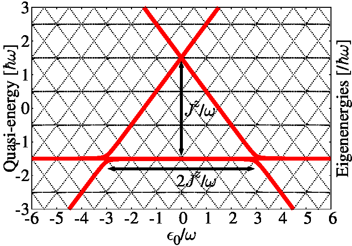
(a) $J^{z}/\omega=-3$

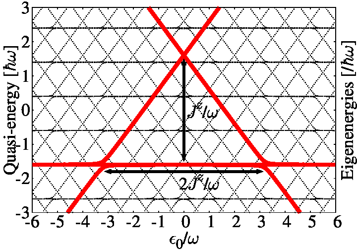
(b) $J^{z}/\omega=-3.2$

Figure 1: Eigenenergies in the absence of driving, $A/\omega=0$ (red lines) and quasienergies for $A/\omega=3.8$ (black lines) as a function of $\epsilon_{0}/\omega$, for the coupling strengths $J^{z}/\omega=-3$ (a) and $J^{z}/\omega=-3.2$ (b) (see Hamiltonian Eq.(7)). Parameters are $\Delta_{1}/\omega=0.1$ and $\Delta_{2}/\omega=0.15$.

Fig.1 shows as a function of the detuning $\epsilon_{0}/\omega$ and for the longitudinal coupling strengths $J^{z}/\omega=-3$ and $J^{z}/\omega=-3.2$, the eigenenergies $E_{i}$, $i=0,...,3$ for the time indepent Hamiltonian (red lines), and in black the quasienergies for the driven Hamiltonian Eq.(7) for $A/\omega=3.8$. We work with the (antiferromagnetic) coupling $J^{z}<0$, which reduces the energy of states $|01\rangle,|10\rangle$ while it increases the energy of states $|00\rangle,|11\rangle$, with $\mathcal{E}=\{|00\rangle,|01\rangle,|10\rangle,|11\rangle\}$ the computational basis in the product space of the two qubits.

The quasienergies display avoided crossings (quasidegeneracies), where the Floquet states are strongly mixed. These quasidegeneracies will play a central role in the structure of the concurrence as we will discuss in the following. In the limit of $\Delta_{i}/\omega\rightarrow 0$, the quasidegeneracies transform in exact crossings of quasienergies, giving the resonance condition $\gamma_{\alpha}-\gamma_{\beta}=n\omega$, $n\in\mathbb{Z}$. Son et al. (2009)

For the present case of longitudinal coupling the quasienergies of the two qubit system computed analytically for $\Delta_{i}/\omega\rightarrow 0$ using the Van Vleck nearly degenerate perturbation theory Son et al. (2009) are $\gamma_{\alpha}\sim\pm\epsilon_{0}+J^{z}/2+m\omega$ and the (quasi) degenerate pair $-J^{z}/2+m\omega$ with $m\in\mathbb{Z}$. As, for $\Delta_{i}/\omega\rightarrow 0$, the driving $\epsilon(t)$ and the static coupling Hamiltonian are both proportional to ${\sigma_{z}}$, the location of the quasi crossings in the spectrum of quasienergies are replicas (in $\pm m\omega$) of the quasi crossings of the static spectrum (see Fig.1). The resonance conditions are thus satisfied respectively for $2\epsilon_{0}\sim n\omega$ and $\epsilon_{0}\pm J^{z}\sim n\omega$, and correspond to multiphoton processes where the population probability is modulated by the zeros of the Bessel functions of order $n$, $J_{n}(A/\omega)=0$.Satanin et al. (2012); Son et al. (2009) Notice that while the first condition gives half integer and integer values of $\epsilon_{0}/\omega$, the second one depends on $J^{z}/\omega$. For integer values of $J^{z}/\omega$ the quasidegeneracies are located at integer values of $\epsilon_{0}/\omega$, as can be clearly seen from Fig.1(a). However, for arbitrary $J^{z}/\omega$, quasi degeneracies also appear for values of $\epsilon_{0}/\omega$ which are neither integer nor half integers (see Fig.1(b)).

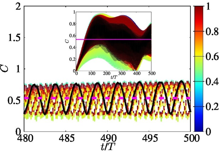
Figure 2: Plots of the concurrence ${C(t,t_{0})}$ for $\epsilon_{0}/\omega=4$ and $A/\omega=3.8$, as a function of the normalized time $t/T$ for $300$ different initial times $t_{0}/T$, represented on the vertical colour bar. The initial state is $|\Psi(t_{0})\rangle$. In black line $\overline{C(t)}$ is plotted and in magenta, its average $\overline{\overline{C}}$. The inset show the plot in the range $t/T\in[0,500]$, while the main figure shows a detail in an interval $t/T\in[480,500]$. Results correspond to inductive coupling with $J^{z}/\omega=-3$, see Eq.(7). The other qubits parameters are the same than in Fig.1.

Fig.2 displays the concurrence $C(t,t_{0})$ as a function of the normalized time $t/T$ calculated for the initial condition $|\Psi(t_{0})\rangle=e^{-iE_{0}t_{0}}|E_{0}\rangle$, which was chosen as the ground state of the time independent Hamiltonian (with eigenvalue $E_{0}$) for detuning energy $\epsilon_{0}/\omega=4$ and static coupling strength $J^{z}/\omega=-3$ (see Fig.1). The driving amplitude chosen is $A/\omega=3.8$. $C(t,t_{0})$ was computed for around $300$ different initial times with $t_{0}/T\in[0,1]$. Notice that due to the different initial times, that induce a different initial phase in the microwave field, the curves are shifted. After averaging over $t_{0}$, $\overline{C}(t)$ (black line), turns out to be a smoother function whose time average $\overline{\overline{C}}$, results independent on time as expected. In the following we will focus on $\overline{\overline{C}}$, which contains the time independent contributions to entanglement dominant for long times.

In Fig.3(a) we show $\overline{\overline{C}}$ as a function of $\epsilon_{0}/\omega$. The initial state is chosen as the ground state for the correspondent $\epsilon_{0}/\omega$, and we keep the same values than in the Fig.2 for the other parameters. In the absence of driving, $A/\omega=0$ (black line), the ground state is entangled for detuning energies satisfying $|\epsilon_{0}/\omega|\lesssim|J^{z}/\omega|=3$, where the concurrence takes values close to $1$. In particular, for $\epsilon_{0}=0$, the ground state is the Bell’s state $(|01\rangle+|10\rangle)/\sqrt{2}$, which is known to be a maximally entangled state.(Wootters, 1998) On the other hand, for values of detuning energy $|\epsilon_{0}/\omega|>|J^{z}/\omega|=3$ the ground state is almost disentangled, i.e. for large values of $\epsilon_{0}$ the ground state is asymptotically a separable state of the computational basis, corresponding to $|00\rangle$ for $\epsilon_{0}\gg 0$ and $|11\rangle$ for $\epsilon_{0}\ll 0$, see Fig.1.

When the driving is turn on ($A/\omega=3.8$), a pattern of resonances is clearly visible in $\overline{\overline{C}}$, where entanglement is either created or destroyed. For $|\epsilon_{0}/\omega|>|J^{z}/\omega|=3$, where the initial condition corresponds to a separable state, we see that it is possible to generate entanglement in a controlled way around a given resonance. Otherwise entanglement is reduced.

The positions of the resonances in $\overline{\overline{C}}$ are determined from the already mentioned conditions: $2\epsilon_{0}/\omega\sim n$ and $\epsilon_{0}/\omega+J^{z}/\omega\sim n$, with $n\in\mathbb{Z}$. Therefore is around a (quasi) degeneracy where the Floquet states can be strongly mixed given rise to significant deviations in the behaviour of the concurrence compared to the undriven case.

Notice that in Fig.3(a), the resonances are at integer and half integer values of $\epsilon_{0}/\omega$, since $J^{z}/\omega=-3$.

In Fig.3(b), we plot $\overline{\overline{C}}$ as a function of $\epsilon_{0}/\omega$ and $A/\omega$, for $J^{z}/\omega=-3$. For a particular multiphoton resonance, the concurrence is modulated by the driving amplitude, where full (or partial) recovery of the initial entanglement is possible.

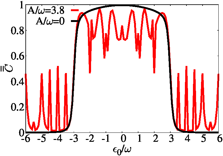
(a)

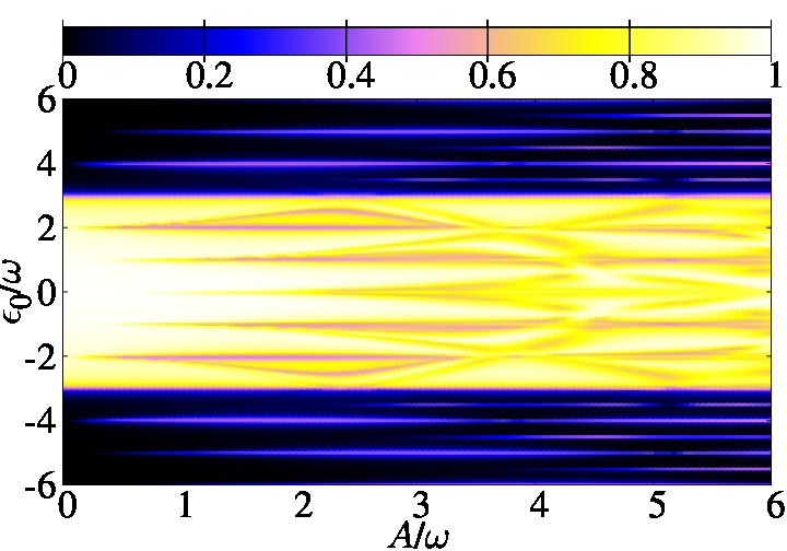
(b)

Figure 3: (a) Plots of $\overline{\overline{C}}$ versus $\epsilon_{0}/\omega$ for $A/\omega=0$ (black line) and $A/\omega=3.8$ (red line). (b) Colour map of $\overline{\overline{C}}$ versus $\epsilon_{0}/\omega$ and $A/\omega$. In both plots the initial condition corresponds to the ground state for the correspondent $\epsilon_{0}/\omega$. $J^{z}/\omega=-3$ is the coupling strength (see Eq.(7)) and other qubits parameters are the same as in Fig. 2.

So far, we have studied the entanglement for a fixed value of the coupling strength. However in practical implementations with flux qubits the intensity of the inductive coupling can be controlled, and it is interesting to analyse whether a different static coupling would induce qualitative changes in the above description, taking into account that the spectrum of quasienergies is sensitive to this change (see Figs.1). In Fig.4 we plot a map of $\overline{\overline{C}}$ versus $J^{z}/\omega$ and $\epsilon_{0}/\omega$ for $A/\omega=0$ and 3.8, respectively, taking as the initial state the ground state for the correspondent $\epsilon_{0}/\omega$ and $J^{z}/\omega$.

(a) $A/\omega=0$

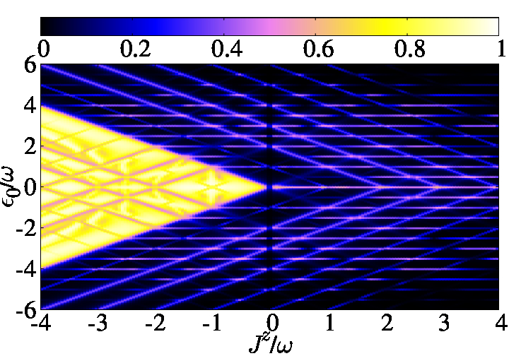
(b) $A/\omega=3.8$

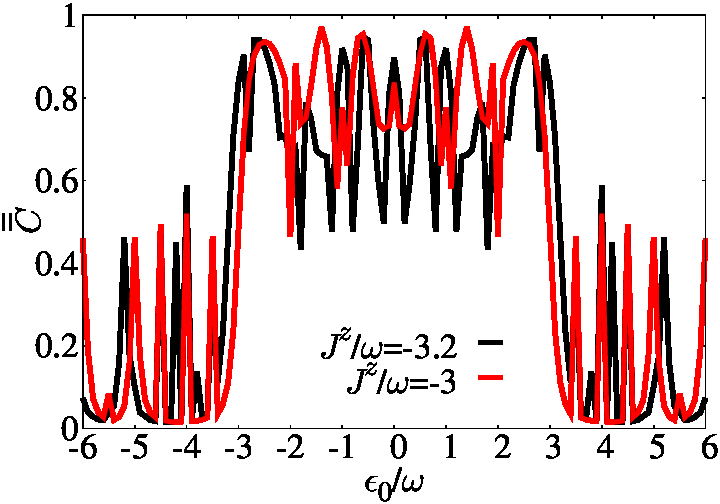
(c) $J^{z}/\omega<0$

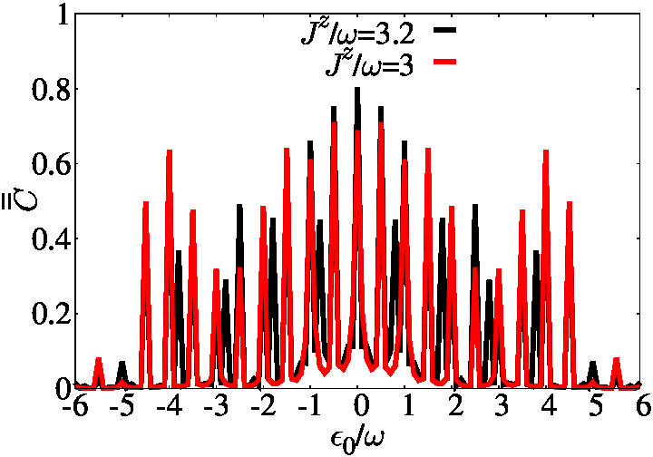
(d) $J^{z}/\omega>0$

Figure 4: Colour map of $\overline{\overline{C}}$ versus $J^{z}/\omega$ and $\epsilon_{0}/\omega$ for $A/\omega=0$ (a) and $A/\omega=3.8$ (b) respectively. $\overline{\overline{C}}$ versus $\epsilon_{0}/\omega$ for $A/\omega=3.8$, for antiferromagnetic (c) and ferromagnetic coupling strengths (d). See text for details.

In the absence of the microwave field (see Fig.4(a)) two well separated behaviours are observed, corresponding to positive and negative values of $J^{z}$ respectively. For $J^{z}<0$ (antiferromagnetic coupling) the ground state is entangled for $|\epsilon_{0}|<|J^{z}|$ as we already described, given rise to the triangular shaped region in $\overline{\overline{C}}$. On the other hand, for the ferromagnetic coupling $J^{z}>0$, which increases the energy of states $|01\rangle,|10\rangle$ and decreases the energy of states $|00\rangle,|11\rangle$, the ground state is entangled only for values $\epsilon_{0}\sim 0$, being approximately the Bell’s state $(|00\rangle+|11\rangle)/\sqrt{2}$. When the microwave field is on, $\overline{\overline{C}}$ exhibits the structure of resonances where the entanglement is created or destroyed in a well controlled way (see Fig.4(b)) with resonances located at half integer or integer values of $\epsilon_{0}/\omega$ and others located at positions determined by the values of $J^{z}/\omega$, as we already mentioned. For integer values of $J^{z}/\omega$ the resonances are at integers $\epsilon_{0}/\omega$, while for arbitrary real values of $J^{z}/\omega$ they are respectively shifted to non integer values of $\epsilon_{0}/\omega$ (notice the straight lines forming the $>$-shaped pattern). These features are clearly observed in Figs.4(c) and 4(d), where $\overline{\overline{C}}$ versus $\epsilon_{0}/\omega$ is plotted for $J^{z}/\omega\lessgtr 0$ and $A/\omega=3.8$.

In Appendix B we derive an expression for a lower bound $C_{I}$ of the averaged concurrence $\overline{\overline{C}}$, that reads:

$$C_{I}=|\sum_{\alpha}\overline{\tilde{C}_{\alpha\alpha}(t)}\sum_{q}|a_{\alpha}(q)|^{2}|<\overline{\overline{C}},$$ (8)

where $a_{\alpha}(q)=\langle u_{\alpha}(q)|\Psi(t_{0})\rangle$ has been already defined and $\overline{\tilde{C}_{\alpha\alpha}(t)}$ is the time average of a Floquet preconcurrence $\tilde{C}_{\alpha\alpha}(t)\equiv\langle u_{\alpha}(t)|^{*}\sigma_{y}^{(1)}\otimes\sigma_{y}^{(2)}|u_{\alpha}(t)\rangle$.

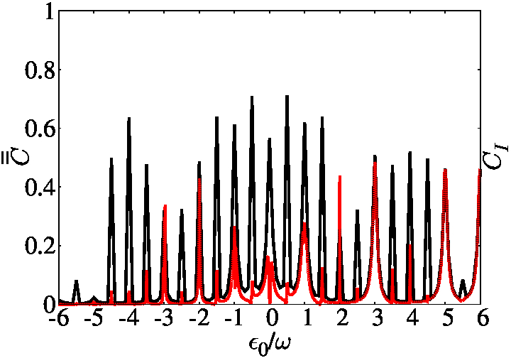
(a)

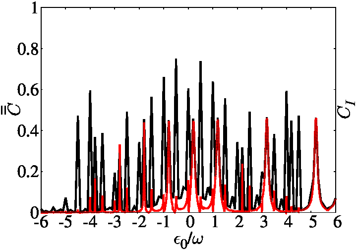
(b)

Figure 5: Plot of $\overline{\overline{C}}$ (black line) and $C_{I}$ (red line) as a function of $\epsilon_{0}/\omega$. In both cases is $A/\omega=3.8$ and the coupling strength $J^{z}/\omega=-3$ (a) and $J^{z}/\omega=-3.2$ (b).

To obtain the above expression for $C_{I}$ we have performed a rotating wave approximation disregarding fast oscillating terms in the concurrence, so we only consider the quasienergies that fulfilled the relation $\gamma_{\alpha}+\gamma_{\beta}=n\omega$, $n\in\mathbb{Z}$ (see Appendix B). In this way $C_{I}$ is mainly governed by the Floquet preconcurrences, each one weighted by the projection of the Floquet states on the initial condition. It should be noted that this expression is useful when the initial state is non entangled, since $C_{I}$ determines the minimal creation of entanglement.

In Fig.5 we plot $\overline{\overline{C}}$ (black line) and $C_{I}$ computed from Eq.(8) (red line), both as a function of $\epsilon_{0}/\omega$. We choose the initial state $|00\rangle$, corresponding to a separable state (of the computational basis), and work with the driven amplitude $A/\omega=3.8$. In Fig.5(a) the coupling strength is $J^{z}/\omega=-3$. The position of the resonances at integer values of $\epsilon_{0}/\omega$ are well captured by the lower bound $C_{I}$, and the agreement with $\overline{\overline{C}}$ is quite good. Notice however that for half integer values of $\epsilon_{0}/\omega$, $\overline{\overline{C}}$ also exhibits resonances that are quite attenuated in $C_{I}$. This behaviour can be understood taking into account that the stationary phase condition employed to compute $C_{I}$ involves the sum $\gamma_{\alpha}+\gamma_{\beta}$ of pairs of quasienergies, which gives either $\epsilon_{0}$ or $J^{z}$. Therefore for integer values of $J^{z}/\omega$ and $\epsilon_{0}/\omega$, the resonance conditions and the stationary phase condition are both satisfied. On the other hand, for half integer values of $\epsilon_{0}/\omega$ the stationary phase approximation is not fulfilled, and the resonances displayed in $\overline{\overline{C}}$ are dimmed in $C_{I}$.

In Fig.5(b) we show a similar plot for $J^{z}/\omega=-3.2$, where some resonances in $\overline{\overline{C}}$ are shifted to non integer values of $\epsilon_{0}/\omega$, as we already discussed. However, due to the stationary phase approximation, $C_{I}$ exhibits well defined resonances only at integer values of $\epsilon_{0}/\omega$. As a consequence, both curves are horizontally displaced respect to each other.

Owing to the contribution of additional terms, $\overline{\overline{C}}$ displays a background structure not observed in $C_{I}$ (see Appendix B).

III.2 Transverse coupling

In this section we focus on the capacitive coupling, see Eq.(2), for which the driven time dependent Hamiltonian reads

$$\hat{H}_{II}(t) =-\frac{1}{2}\sum_{i=1}^{2}\left(\epsilon_{i}(t)\sigma_{z}^{(i)}+\Delta_{i}\sigma_{x}^{(i)}\right)$$ (9)

$$-\frac{J^{c}}{2}((1-p)\sigma_{x}^{(1)}\otimes\sigma_{x}^{(2)}+p\sigma_{y}^{(1)}\otimes\sigma_{y}^{(2)}),$$

where $p\in\mathbb{R}$ is a real number, and the other quantities have been already defined.

(a) $p=0.5$

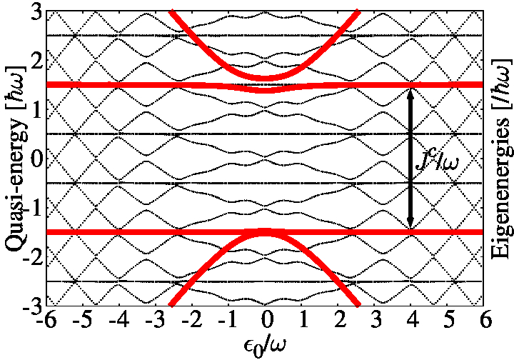
(b) $p=0$

Figure 6: Energy levels for $A/\omega=0$ (red lines) and quasienergies for $A/\omega=3.8$ (black lines) as a function of $\epsilon_{0}/\omega$ for $J^{c}/\omega=-3$, see Hamiltonian Eq.( 9), with $p=0.5$ (a) and $p=0$ (b). The qubits parameters are the same as in previous figures.

Figure 6 shows the eigenenergies $E^{\prime}_{i}$, $i=0,...,3$, as a function of $\epsilon_{0}/\omega$ for the static Hamiltonian for $p=0.5$ (Fig.6(a)) and $p=0$ (Fig. 6(b)), in both cases for the coupling strength $J^{c}/\omega=-3$.

The coupling Hamiltonian for $p=0.5$ represents the excitation exchange interaction which mixes the states $|01\rangle,|10\rangle$ breaking the former degeneracy present in the absence of coupling. For $p=0$ the coupling Hamiltonian is $\hat{H}^{c}_{12}=J^{c}/2\sigma_{x}^{(1)}\otimes\sigma_{x}^{(2)}$, which includes the excitation exchange interaction and the magnetization-changing terms. Sauer et al. (2012) In this case the coupling breaks the former degeneracy between $|01\rangle,|10\rangle$ but also mixes the states $|00\rangle$ and $|11\rangle$, given rise to the spectrum exhibited in Fig.6(b).

Additionally we plot the quasienergies for the driven Hamiltonian Eq.(9) in black lines, for the amplitude $A/\omega=3.8$. Notice that while for $p=0.5$ the driving field along $\sigma_{z}$ and the coupling Hamiltonian commute, as it can be checked from the properties of the Pauli matrices, for $p=0$ they do not. As a consequence, the spectrum of quasienergies if Fig.6(b) has a non trivial structure.

The quasienergies can be obtained for arbitrary amplitudes of the driving field for $p=0.5$ using perturbation theory for $\Delta_{i}/\omega\rightarrow 0$, as we have done for the longitudinal coupling in Sec.III.1. For the present case we get $\gamma_{\alpha}\sim\pm\epsilon_{0}+m\omega$ and $\pm J^{c}/2+m\omega$. Therefore the resonance conditions are satisfied for $\epsilon_{0}/\omega+J^{c}/2\omega\sim n$, $2\epsilon_{0}/\omega\sim n$ and $J^{c}/\omega\sim n$ (independent of the detuning), being quite similar to the inductive case.

However for the $p=0$ case, the additional limit $A/\omega\rightarrow 0$ has to be taken in order to get analytical expressions for the quasienergies $\gamma_{\alpha}\sim\pm\sqrt{\epsilon_{0}^{2}+(J_{c}/2)^{2}}+m\omega$ and $\pm J^{c}/2+m\omega$. Thus the resonance conditions are fulfilled, in this limit, for $J^{c}/\omega\sim n$ (independent of the detuning), for values satisfying $(2\epsilon_{0}/\omega)^{2}+(J^{c}/\omega)^{2}\sim n^{2}$ and for $J^{c}/2\omega\pm\sqrt{(\epsilon_{0}/\omega)^{2}+(J^{c}/2\omega)^{2}}\sim n$. The two latter relations give rise to an intricate pattern of quasidegeneracies in the spectrum of Fig.6(b), that will induce a non trivial behaviour in the concurrence.

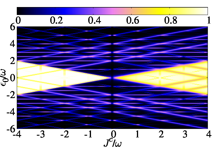
Figure 7: Colour map of $\overline{\overline{C}}$ versus $J^{c}/\omega$ and $\epsilon_{0}/\omega$ for the capacitive coupling with $p=0.5$, see Hamiltonian Eq.(9).The driving amplitude is $A/\omega=3.8$ (see text for more details).

We start by analyzing the concurrence for the symmetric case $p=0.5$ where the response is quite similar to the inductive coupling case previously studied. In Fig. 7 we plot $\overline{\overline{C}}$ versus $J^{c}/\omega$ and $\epsilon_{0}/\omega$ when the driving amplitude is $A/\omega=3.8$ taking as initial condition the ground state for each value of the detuning. It is evident that the pattern of resonances where entanglement is created or destroyed resembles the inductive case.

However, the symmetric transverse coupling mixes the states $|01\rangle,|10\rangle$ independently of the sign of the coupling strength $J^{c}$, given rise to similar ground states for both $J^{c}/\omega\lessgtr 0$, see Fig.6(a). Consequently the concurrence exhibits a quite symmetric pattern of resonances both in $J^{c}/\omega$ and $\epsilon_{0}/\omega$, unlike the inductive studied in Sec. III.1.

For other values of the parameter $p\neq 0.5$, we expect a non trivial behaviour of the concurrence due to the much richer structure of the spectrum of quasienergies.

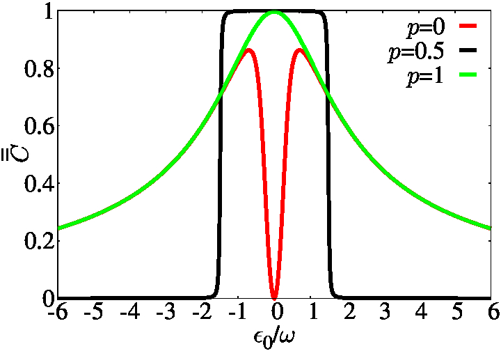
(a) $A/\omega=0$

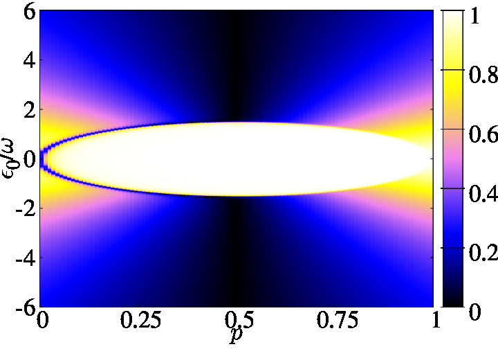
(b) $A/\omega=0$

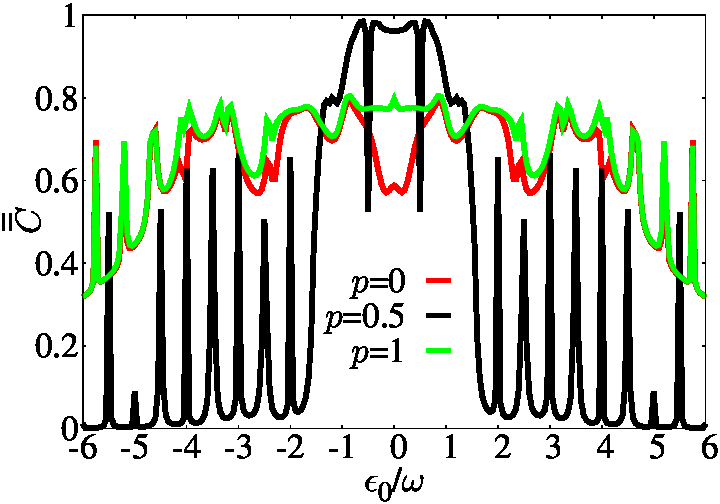
(c) $A/\omega=3.8$

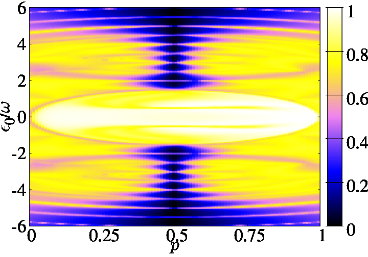
(d) $A/\omega=3.8$

Figure 8: Plot of $\overline{\overline{C}}$ as a function of $\epsilon_{0}/\omega$ for $A/\omega=0$ (a) and $A/\omega=3.8$ (c). $p=0$ (red line), $p=0.5$ (black line) and $p=1$ (green line). Colour map of $\overline{\overline{C}}$ as a function of $\epsilon_{0}/\omega$ and $p$ for $A/\omega=0$ (b) and $A/\omega=3.8$ (d) respectively. In all the cases the initial condition is the ground state $|E^{\prime}_{0}\rangle$. See text for more details.

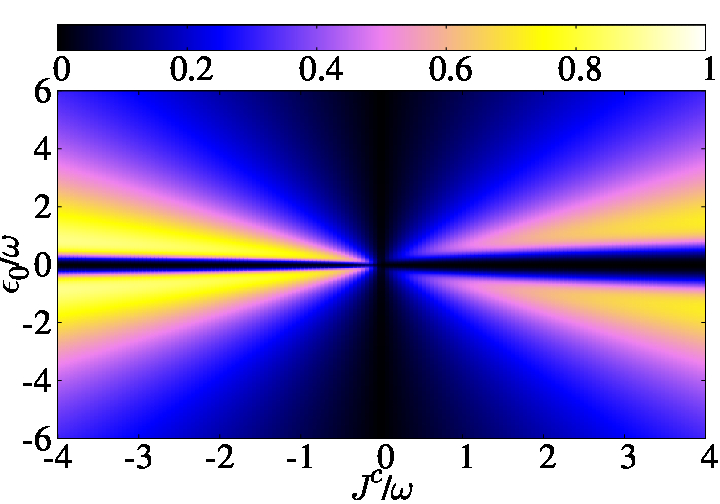
(a) $A/\omega=0$

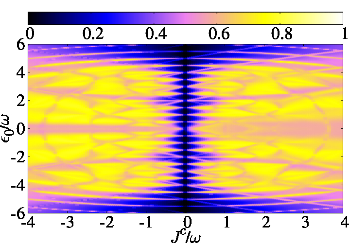
(b) $A/\omega=3.8$

Figure 9: Colour map of $\overline{\overline{C}}$ versus $J^{c}/\omega$ and $\epsilon_{0}/\omega$ for the capacitive coupling $p=0$, see Hamiltonian Eq.(9).The driving amplitudes are $A/\omega=0$ (a) and $A/\omega=3.8$ (b). The initial condition is $|E^{\prime}_{0}\rangle$.(see text for details.

In Fig.8(a) we show $\overline{\overline{C}}$ without driving for a fixed value $J^{c}/\omega=-3$. For $p=0$ (red line) the ground state is separable for $\epsilon_{0}=0$, corresponding to the singlet state $|s_{1}\rangle|s_{2}\rangle$, with $|s_{i}\rangle=(|0\rangle_{i}+|1\rangle_{i})/\sqrt{2}$. On the other hand, for $\epsilon_{0}\neq 0$ the ground state is entangled and thus the concurrence increases as the states become mixed. However for larger values of $\epsilon_{0}$ the state goes asymptotically to a separable state (see Fig.6(b)).

For the $p=1$ (green line) the ground state is maximally entangled for $\epsilon_{0}=0$, but the concurrence decreases as $\epsilon_{0}$ increases, analogously to the $p=0$ case. For completeness we include the coupling $p=0.5$ already studied (black line).

Figure8(c) shows $\overline{\overline{C}}$ when the driving is on for an amplitude of $A/\omega=3.8$ and $J^{c}/\omega=-3$. For $p=0$ the entanglement is created in a wide range of $\epsilon_{0}/\omega$, specially near of $\epsilon_{0}=0$ where the initial state is a separable state (corresponding to a singlet state). For $p=1$ (green line) the entanglement is reduced near $\epsilon_{0}=0$. For larger values of $\epsilon_{0}/\omega$ we observe in both cases a quite similar pattern, with the creation of entanglement due to the driving, but with wider resonances compared to $p=0.5$ case. This is in agreement with the landscape of avoided crossings in the spectrum of quasienergies, due to the non commutation of the static Hamiltonian with the driving field.

The wider resonances generate a region where entanglement is quite robust to changes in the flux detuning. This could be a tool to stabilize the entanglement created by the driving field. In this way, it is interesting to extend the analysis studying the dependence of $\overline{\overline{C}}$ on $p$ and $\epsilon_{0}/\omega$. Fig. 8(b) shows the results without driving for $J^{c}/\omega=-3$. Two well defined regions can be observed where there is a qualitative change in the behaviour of the concurrence. For $0<p<0.5$ the coupling $J^{c}/2\sigma_{x}^{(1)}\otimes\sigma_{x}^{(2)}$ is the dominant term. In this case, for $\epsilon_{0}\sim 0$ the ground state is separable corresponding to the singlet states $|s_{1}\rangle|s_{2}\rangle$, but as $p$ increases it also does the term $J^{c}/2\sigma_{y}^{(1)}\otimes\sigma_{y}^{(2)}$, and the ground state becomes entangled. For the region $0.5<p<1$ the dominant term is $J^{c}/2\sigma_{y}^{(1)}\otimes\sigma_{y}^{(2)}$ and in this case the ground state remains maximally entangled near $\epsilon_{0}\sim 0$ as $p$ decreases. In Fig.8(d) we present the results for driving amplitude $A/\omega=3.8$, where important creation of entanglement with a rich (and non trivial) pattern of wide resonances is clearly observed in an ample range of $p\neq 0.5$.

From the previous analysis it should be clear that although for the symmetric case ($p=0.5$) the resonances are well defined and sharp, it could be interesting to profit from wider resonances created for other values of $p$, in order to control the entanglement induced by the driving field.

Besides changing the dominant interaction in the coupling Hamiltonian, one can analize the sensitivity of the concurrence with the coupling strength for a fix value of $p$. As an example we focus on the $p=0$ case. The pattern displayed in Fig. 9(a) in the absence of driving is consistent with the resonant conditions obtained previously for $(\Delta_{i},A)\rightarrow 0$. In particular notice the regions where the quasi linear behaviour with $J^{c}/\omega$ dominates for $\epsilon_{0}/\omega\thicksim 0$, turning into parabolic ones in the plane $(\epsilon_{0}/\omega,J^{c}/\omega)$, for larger values of the flux detuning. The concurrence takes different values along these regions, even for a fixed $J^{c}/\omega$. The driving induces a drastic change in this behaviour. Unlike the longitudinal coupling or the symmetric transverse coupling case, where the behaviour with $J^{c}/\omega$ for finite driving was quite predictable, we here observe non trivial features. Among others, is the generation of an important amount of ${\it homogeneous}$ entanglement for a wide range of flux detuning and static coupling strength.

Additionally the concurrence exhibits a rather symmetric pattern for $J^{c}/\omega\lessgtr 0$, similarly to the symmetric transverse coupling case.

IV Conclusions

In this work we have shown that entanglement can be manipulated by external periodic driving fields. In particular we presented extensive numerical and analytical results for the concurrence of a system composed by two coupled flux qubits driven by an external ac magnetic flux.

The main result is that when the system is tuned at or near a multiphoton resonance full control of entanglement is possible: (a) when the initial state is disentangled one can drive it towards a highly entangled state, and (b) when the initial state is entangled one can strongly reduce entanglement with the driving.

In the special cases when the driving term in the Hamiltonian and the interaction term in the Hamiltonian commute (longitudinal coupling and symmetric $p=0.5$ transverse coupling), the entanglement control region is within a narrow range of the multiphoton resonances. This shows, for example, as well-defined lines of “entanglement resonance ” in the $\left\{\epsilon_{0},J^{z}(J^{c})\right\}$ plane in Fig.4(b) and Fig.7. One advantage of this case is that once the resonance is exactly tuned, the control of entanglement is almost complete.

In the more common case where the driving Hamiltonian and the interaction Hamiltonian do not commute (as shown here for the $p=0$ transverse coupling), the multiphoton resonances, as seen in terms of an entanglement measure, are wide and nearly overlap. In the $\left\{\epsilon_{0},J^{c}\right\}$ plane in Fig.9(b) this shows as broad regions where entanglement can be enhanced starting from a disentangled initial condition. In this case, the control of entanglement is more robust in parameter space without the need to fine tune at a resonance. This suggests that fabricating flux qubits that interact through a capacitive (transverse) coupling will be more convenient for entanglement control through ac driving.

Acknowlegments

We acknowledge support from CNEA, CONICET, UNCuyo (P 06/C455) and ANPCyT (PICT2014-1382).

Appendix A Concurrence in Floquet basis

As it was presented in section II, the hamiltonian 1 driven by the microwave field, $\epsilon_{i}(t)=\epsilon_{i}+A_{i}\cos(\omega t)$, is periodic in time $\hat{H}(t)=\hat{H}(t+T)$, $T=2\pi/\omega$. So we shall work under the Floquet formalism Shirley (1965).

Given the global wave function of the system $|\Psi(t)\rangle$, its evolution is governed by the Shrödinger equation

$$\hat{H}(t)|\Psi(t)\rangle=i\hbar\frac{\partial}{\partial t}|\Psi(t)\rangle.$$ (10)

We can spanned $|\Psi(t)\rangle$ in the Floquet basis

$$|\Psi(t)\rangle=\sum_{\alpha}a_{\alpha}(t_{0})e^{-i\gamma_{\alpha}t/\hbar}|u_{\alpha}(t)\rangle,$$ (11)

where $|u_{\alpha}(t)\rangle=|u_{\alpha}(t+T)\rangle$ is the Floquet state with its respective quasienergy $\gamma_{\alpha}$, $\alpha$ the system index, $a_{\alpha}(t_{0})=\langle u_{\alpha}(t_{0})|\Psi(t_{0})\rangle$ and $|\Psi(t_{0})\rangle$ the initial condition. If we replace the Eq. 11 into 10 we obtain

$$(H(t)-i\hbar\frac{\partial}{\partial t})|u_{\alpha}(t)\rangle=\gamma_{\alpha}|u_{\alpha}(t)\rangle$$ (12)

Solving this equation we obtain the evolution of $|u_{\alpha}(t)\rangle$. It is straightforward to see that the shift $\gamma_{\alpha}\rightarrow\gamma_{\alpha}+n\omega$, $n\in\mathbb{Z}$, leaves unchaged the Eq. 12 since the quasienergies $\gamma_{\alpha}$ and $\gamma_{\alpha}+n\omega$ correspond to the Floquet states $|u_{\alpha}(t)\rangle$ and $e^{-in\omega t}|u_{\alpha}(t)\rangle$, respectively.

Now we can calculate the concurrence $C(t,t_{0})=|\langle\Psi(t)|^{*}|\sigma_{y}^{(1)}\otimes\sigma_{y}^{(2)}|\Psi(t)\rangle$, presented in Sec. II. Using the expantion $|\Psi(t)\rangle$ in the Floquet basis, we obtain

$$C(t,t_{0})=|\sum_{\alpha\beta}a_{\alpha}(t_{0})a_{\beta}(t_{0})e^{-i(\gamma_{\alpha}+\gamma_{\beta})(t-t_{0})}\tilde{C}_{\alpha\beta}(t)|,$$ (13)

with $\gamma_{{}^{\alpha}_{\beta}}$ the quasienergies, $a_{{}^{\alpha}_{\beta}}(t_{0})=\langle u_{{}^{\alpha}_{\beta}}(t_{0})|\Psi(t_{0})\rangle$, $|\Psi(t_{0})\rangle$ the initial condition and $\tilde{C}_{\alpha\beta}(t)=\langle u_{\alpha}(t)|^{*}\sigma_{y}\otimes\sigma_{y}|u_{\beta}(t)\rangle$. We shall take $\hbar=1$.

Using the extended Fourier basis $|u_{\alpha}(t)\rangle=\sum_{k}e^{-ik\omega t}|u_{\alpha}(k)\rangle$ and $\langle u_{\alpha}(t_{0})|=\sum_{q}e^{iq\omega t}\langle u_{\alpha}(q)|$, the Eq. 13 remains like

$$C(t,t_{0})=\lvert\sum_{\alpha\beta kk^{\prime}qq^{\prime}}\tilde{C}_{\alpha\beta}(k,k^{\prime})f_{\alpha\beta}(q,q^{\prime})e^{-i\varphi_{\alpha\beta}^{kk^{\prime}qq^{\prime}}(t,t_{0})}\arrowvert,$$ (14)

where $\varphi_{\alpha\beta}^{kk^{\prime}qq^{\prime}}(t,t_{0})=(\gamma_{\beta}+\gamma_{\alpha}-(k^{\prime}+k)\omega)t-(\gamma_{\beta}+\gamma_{\alpha}-(q^{\prime}+q)\omega)t_{0}$ with $\gamma_{{}^{\alpha}_{\beta}}$ the quasienergies, $\tilde{C}_{\alpha\beta}(k,k^{\prime})=\langle u_{\alpha}(k)|^{*}\sigma_{y}\otimes\sigma_{y}|u_{\beta}(k^{\prime})\rangle$ and $f_{\alpha\beta}(q,q^{\prime})=a_{\alpha}(q)a_{\beta}(q^{\prime})$, with $a_{{}^{\alpha}_{\beta}}(^{q}_{q^{\prime}})=\langle u_{{}^{\alpha}_{\beta}}(^{q}_{q^{\prime}})|\Psi(t_{0})\rangle$.

Appendix B Lower bound for time-averaged concurrence

Here we calculate a lower bound for the average concurrence $\overline{\overline{C}}$. First we expand the Eq. 14 as

$$C(t,t_{0})=\lvert\sum_{\alpha\beta kk^{\prime}qq^{\prime}}\tilde{C}_{\alpha\beta}(k,k^{\prime})f_{\alpha\beta}(q,q^{\prime})\cos(\varphi_{\alpha\beta}^{kk^{\prime}qq^{\prime}}(t,t_{0})$$ (15)

$$+i\sum_{\alpha\beta kk^{\prime}qq^{\prime}}\tilde{C}_{\alpha\beta}(k,k^{\prime})f_{\alpha\beta}(q,q^{\prime})\sin(\varphi_{\alpha\beta}^{kk^{\prime}qq^{\prime}}(t,t_{0}))\arrowvert$$

where we separe it in the real ($Re$) and imaginarie ($Im$) part. Second, using the relations $|z|\geq|Re(z)|,|Im(z)|$, for a complex number $z\in\mathbb{C}$, the Eq. 15 is changed to

$$C(t,t_{0}) \geq\lvert\sum_{\alpha\beta kk^{\prime}qq^{\prime}}\tilde{C}_{\alpha\beta}(k,k^{\prime})f_{\alpha\beta}(q,q^{\prime})\cos(\varphi_{\alpha\beta}^{kk^{\prime}qq^{\prime}}(t,t_{0})\arrowvert,$$ (16)

$$C(t,t_{0}) \geq\lvert\sum_{\alpha\beta kk^{\prime}qq^{\prime}}\tilde{C}_{\alpha\beta}(k,k^{\prime})f_{\alpha\beta}(q,q^{\prime})\sin(\varphi_{\alpha\beta}^{kk^{\prime}qq^{\prime}}(t,t_{0}))\arrowvert,$$

Now we apply the inequality $\int_{a}^{b}|f(x)|dx\geq|\int_{a}^{b}f(x)dx|$, with $f(x):\mathbb{R}\rightarrow\mathbb{R}$ and $a<b$, to the Eq. 16. Here we are inferiorly limiting $\overline{\overline{C}}=\frac{1}{T}\int_{0}^{T}dt\frac{1}{T}\int_{0}^{T}dt_{0}C(t,t_{0})$. Then we obtain two lower bounds $\overline{\overline{C}}\geq C_{I},C_{II}$ such as

$$C_{I} =\lvert\sum_{\alpha\beta kk^{\prime}qq^{\prime}}\tilde{C}_{\alpha\beta}(k,k^{\prime})f_{\alpha\beta}(q,q^{\prime})\overline{\overline{\cos(\varphi_{\alpha\beta}^{kk^{\prime}qq^{\prime}}(t,t_{0})}}\arrowvert,$$ (17)

$$C_{II} =\lvert\sum_{\alpha\beta kk^{\prime}qq^{\prime}}\tilde{C}_{\alpha\beta}(k,k^{\prime})f_{\alpha\beta}(q,q^{\prime})\overline{\overline{\sin(\varphi_{\alpha\beta}^{kk^{\prime}qq^{\prime}}(t,t_{0}))}}\arrowvert.$$

Using the trigonometric identities $\sin(A-B)=\sin(A)\cos(B)-\cos(A)\sin(B)$ and $\cos(A-B)=\cos(A)\cos(B)+\sin(A)\sin(B)$, and taking the average over $t,t_{0}$ we obtain

$$\overline{\overline{\cos(\varphi_{\alpha\beta}^{kk^{\prime}qq^{\prime}}(t,t_{0}))}} =\delta_{\gamma_{\alpha}+\gamma_{\beta}-n\omega,0}\,\delta_{\gamma_{\alpha}+\gamma_{\beta}-m\omega,0}$$ (18)

$$+\delta_{\gamma_{\alpha}+\gamma_{\beta}-n\omega,\pi/(2T)}\,\delta_{\gamma_{\alpha}+\gamma_{\beta}-m\omega,\pi/(2T)},$$

$$\overline{\overline{\sin(\varphi_{\alpha\beta}^{kk^{\prime}qq^{\prime}}(t,t_{0}))}} =\delta_{\gamma_{\alpha}+\gamma_{\beta}-n\omega,\pi/(2T)}\,\delta_{\gamma_{\alpha}+\gamma_{\beta}-m\omega,0}$$

$$-\delta_{\gamma_{\alpha}+\gamma_{\beta}-n\omega,0}\,\delta_{\gamma_{\alpha}+\gamma_{\beta}-m\omega,\pi/(2T)},$$

with $n=k+k^{\prime}$ and $m=q+q^{\prime}$. Replacing $T=2\pi/\omega$ and ordening the terms, we obtain

$$\overline{\overline{\cos(\varphi_{\alpha\beta}^{kk^{\prime}qq^{\prime}}(t,t_{0}))}} =\delta_{\gamma_{\alpha}+\gamma_{\beta},n\omega}\,\delta_{\gamma_{\alpha}+\gamma_{\beta},m\omega}$$ (19)

$$+\delta_{\gamma_{\alpha}+\gamma_{\beta},(n+1/4)\omega}\,\delta_{\gamma_{\alpha}+\gamma_{\beta},(m+1/4)\omega},$$

$$\overline{\overline{\sin(\varphi_{\alpha\beta}^{kk^{\prime}qq^{\prime}}(t,t_{0}))}} =\delta_{\gamma_{\alpha}+\gamma_{\beta},(n+1/4)\omega}\,\delta_{\gamma_{\alpha}+\gamma_{\beta},m\omega}$$

$$-\delta_{\gamma_{\alpha}+\gamma_{\beta},n\omega}\,\delta_{\gamma_{\alpha}+\gamma_{\beta},(m+1/4)\omega}.$$

We suppose the main contribution to concurrence is near the resonances condition $\gamma_{\alpha}+\gamma_{\beta}=n\omega$, this is equivalent to a rotating wave approximation disregarding fast oscillating terms. The averages over $t,t_{0}$ remain

$$\overline{\overline{\cos(\varphi_{\alpha\beta}^{kk^{\prime}qq^{\prime}}(t,t_{0}))}} \sim\delta_{\gamma_{\alpha}+\gamma_{\beta},n\omega}\,\delta_{\gamma_{\alpha}+\gamma_{\beta},m\omega},$$ (20)

$$\overline{\overline{\sin(\varphi_{\alpha\beta}^{kk^{\prime}qq^{\prime}}(t,t_{0}))}} \sim 0.$$

Using the last result we obtain $\overline{\overline{C}}\geq C_{I}\geq C_{II}=0$, then the corresponding lower bound expression is

$$C_{I}\sim\lvert\sum_{{}^{\alpha\beta}_{knqm}}\tilde{C}_{\alpha\beta}(k,n-k)f_{\alpha\beta}(q,m-q)\delta_{\gamma_{\alpha}+\gamma_{\beta},n\omega}\,\delta_{\gamma_{\alpha}+\gamma_{\beta},m\omega}\arrowvert,$$ (21)

Given the Eq.21, it is necessary evaluate the condition $\gamma_{\beta}=-\gamma_{\alpha}+n\omega$ (also $m$) on the involved Floquet states. We know that for a given Floquet state $|u_{\beta}(t)\rangle$ its evolution is governed by $e^{-i\gamma_{\beta}}|u_{\beta}(t)\rangle$. Therefore considering the resonance condition we obtain

$$e^{-i\gamma_{\beta}}|u_{\beta}(t)\rangle =e^{i\gamma_{\alpha}}e^{-in\omega}|u_{\beta}(t)\rangle,$$ (22)

$$=e^{i\gamma_{\alpha}}e^{-in\omega}\sum_{k}e^{ik\omega t}|u_{\beta}(k)\rangle$$

$$=e^{i\gamma_{\alpha}}\sum_{k}e^{i(k-n)\omega t}|u_{\beta}(k)\rangle$$

$$=e^{i\gamma_{\alpha}}\sum_{k}e^{ik\omega t}|u_{\beta}(k-n)\rangle$$

$$=e^{i\gamma_{\alpha}}\sum_{k}e^{-ik\omega t}|u_{\beta}(n-k)\rangle.$$

For another part, we can compare the last result to $(e^{-i\gamma_{\alpha}}|u_{\alpha}(t)\rangle)^{*}$, where

$$(e^{-i\gamma_{\alpha}}|u_{\alpha}(t)\rangle)^{*} =e^{i\gamma_{\alpha}}|u_{\alpha}(t)\rangle^{*},$$ (23)

$$=e^{i\gamma_{\alpha}}\sum_{k}e^{-ik\omega t}|u_{\alpha}(k)\rangle^{*}$$

$$=e^{i\gamma_{\alpha}}\sum_{k}e^{-ik\omega t}|u_{\alpha}(-k)\rangle.$$

Then, from Eq.22 and 23, we obtain an equivalence relation:

$$\gamma_{\beta}\rightarrow-\gamma_{\alpha}+n\omega\Rightarrow|u_{\beta}(n-k)\rangle\rightarrow|u_{\alpha}(-k)\rangle.$$ (24)

Using the result 24 with $n=k+k^{\prime}$ and $m=q+q^{\prime}$, the lower bound in Eq. 21 remains like

$$C_{I} \sim|\sum_{\alpha kq}\tilde{C}_{\alpha\alpha}(k,-k)f_{\alpha\alpha}(q,-q)|,$$ (25)

where $\tilde{C}_{\alpha\alpha}(k,-k)=\langle u_{\alpha}(k)|^{*}\sigma_{y}\otimes\sigma_{y}|u_{\alpha}(-k)\rangle$ and $f_{\alpha\alpha}(q,-q)=a_{\alpha}(q)a_{\alpha}(-q)$, with $a_{\alpha}(q)=\langle u_{\alpha}(q)|\Psi(t_{0})\rangle$.

From Eq.25, we identify a contribution of the form

$$\sum_{k}\tilde{C}_{\alpha\beta}(k,-k) =\frac{1}{T}\int_{0}^{T}dt\,\tilde{C}_{\alpha\alpha}(t)=\overline{\tilde{C}_{\alpha\alpha}(t)},$$ (26)

where $\tilde{C}_{\alpha\alpha}(t)=\langle u_{\alpha}(t)|^{*}\sigma_{y}\otimes\sigma_{y}|u_{\alpha}(t)\rangle$ is the Floquet preconcurrence. Also, using the property $|u_{\alpha}(-q)\rangle=|u_{\alpha}(q)\rangle^{*}$ we obtain

$$f_{\alpha\alpha}(-q,q)=a_{\alpha}(-q)a_{\alpha}(q)=a^{*}_{\alpha}(q)a_{\alpha}(q)=|a_{\alpha}(q)|^{2},$$ (27)

corresponding to the amplitude of the Floquet states projections over the initial condition.

Finally remplacing equations 26 and 27 in 25 we obtain

$$C_{I} \sim|\sum_{\alpha}\overline{\tilde{C}_{\alpha\alpha}(t)}\sum_{q}|a_{\alpha}(q)|^{2}|,$$ (28)

This expression is useful for a non-entangled initial state since it represents the minimal entanglement creation.

References

- Orlando et al. (1999) T. P. Orlando, J. E. Mooij, L. Tian, C. H. van der Wal, L. S. Levitov, S. Lloyd, and J. J. Mazo, Phys. Rev. B 60, 15398 (1999).
- Friedman et al. (2000) J. R. Friedman, V. Patel, W. Chen, S. K. Tolpygo, and J. E. Lukens, Nature 406, 43 (2000).
- van der Wal et al. (2000) C. H. van der Wal, A. C. J. ter Haar, F. K. Wilhelm, R. N. Schouten, C. J. P. M. Harmans, T. P. Orlando, S. Lloyd, and J. E. Mooij, Science 290, 773 (2000), http://science.sciencemag.org/content/290/5492/773.full.pdf .
- Martinis et al. (2002) J. M. Martinis, S. Nam, J. Aumentado, and C. Urbina, Phys. Rev. Lett. 89, 117901 (2002).
- Oliver et al. (2005) W. D. Oliver, Y. Yu, J. C. Lee, K. K. Berggren, L. S. Levitov, and T. P. Orlando, Science 310, 1653 (2005), http://science.sciencemag.org/content/310/5754/1653.full.pdf .
- Majer et al. (2005) J. B. Majer, F. G. Paauw, A. C. J. ter Haar, C. J. P. M. Harmans, and J. E. Mooij, Phys. Rev. Lett. 94, 090501 (2005).
- Strauch et al. (2003) F. W. Strauch, P. R. Johnson, A. J. Dragt, C. J. Lobb, J. R. Anderson, and F. C. Wellstood, Phys. Rev. Lett. 91, 167005 (2003).
- Izmalkov et al. (2004) A. Izmalkov, M. Grajcar, E. Il’ichev, T. Wagner, H.-G. Meyer, A. Y. Smirnov, M. H. S. Amin, A. M. van den Brink, and A. M. Zagoskin, Phys. Rev. Lett. 93, 037003 (2004).
- Grajcar et al. (2005) M. Grajcar, A. Izmalkov, S. H. W. van der Ploeg, S. Linzen, E. Il’ichev, T. Wagner, U. Hübner, H.-G. Meyer, A. Maassen van den Brink, S. Uchaikin, and A. M. Zagoskin, Phys. Rev. B 72, 020503 (2005).
- Yamamoto et al. (2003) T. Yamamoto, Y. A. Pashkin, O. Astafiev, Y. Nakamura, and J. S. Tsai, Nature 425, 941 (2003).
- Mooij et al. (1999) J. E. Mooij, T. P. Orlando, L. Levitov, L. Tian, C. H. van der Wal, and S. Lloyd, Science 285, 1036 (1999), http://science.sciencemag.org/content/285/5430/1036.full.pdf .
- van der Ploeg et al. (2007) S. H. W. van der Ploeg, A. Izmalkov, A. M. van den Brink, U. Hübner, M. Grajcar, E. Il’ichev, H.-G. Meyer, and A. M. Zagoskin, Phys. Rev. Lett. 98, 057004 (2007).
- Wendin and Shumeiko (2005) G. Wendin and V. Shumeiko, (2005).
- Plourde et al. (2004) B. L. T. Plourde, J. Zhang, K. B. Whaley, F. K. Wilhelm, T. L. Robertson, T. Hime, S. Linzen, P. A. Reichardt, C.-E. Wu, and J. Clarke, Phys. Rev. B 70, 140501 (2004).
- Harrabi et al. (2009) K. Harrabi, F. Yoshihara, A. O. Niskanen, Y. Nakamura, and J. S. Tsai, Phys. Rev. B 79, 020507 (2009).
- de Groot et al. (2010) P. C. de Groot, J. Lisenfeld, R. N. Schouten, S. Ashhab, A. Lupascu, C. J. P. M. Harmans, and J. E. Mooij, Nat Phys 6, 763 (2010).
- Shevchenko et al. (2010) S. Shevchenko, S. Ashhab, and F. Nori, Physics Reports 492, 1 (2010).
- Berns et al. (2006) D. M. Berns, W. D. Oliver, S. O. Valenzuela, A. V. Shytov, K. K. Berggren, L. S. Levitov, and T. P. Orlando, Phys. Rev. Lett. 97, 150502 (2006).
- Rudner et al. (2008) M. S. Rudner, A. V. Shytov, L. S. Levitov, D. M. Berns, W. D. Oliver, S. O. Valenzuela, and T. P. Orlando, Phys. Rev. Lett. 101, 190502 (2008).
- Izmalkov et al. (2008) A. Izmalkov, S. H. W. van der Ploeg, S. N. Shevchenko, M. Grajcar, E. Il’ichev, U. Hübner, A. N. Omelyanchouk, and H.-G. Meyer, Phys. Rev. Lett. 101, 017003 (2008).
- Ferrón et al. (2010) A. Ferrón, D. Domínguez, and M. J. Sánchez, Phys. Rev. B 82, 134522 (2010).
- Oliver and Valenzuela (2009) W. D. Oliver and S. O. Valenzuela, Quantum Information Processing 8, 261 (2009).
- Shirley (1965) J. H. Shirley, Phys. Rev. 138, B979 (1965).
- Ferrón et al. (2012) A. Ferrón, D. Domínguez, and M. J. Sánchez, Phys. Rev. Lett. 109, 237005 (2012).
- Ferrón et al. (2016) A. Ferrón, D. Domínguez, and M. J. Sánchez, Phys. Rev. B 93, 064521 (2016).
- Sauer et al. (2012) S. Sauer, F. Mintert, C. Gneiting, and A. Buchleitner, Journal of Physics B: Atomic, Molecular and Optical Physics 45, 154011 (2012).
- Son et al. (2009) S.-K. Son, S. Han, and S.-I. Chu, Phys. Rev. A 79, 032301 (2009).
- Hausinger and Grifoni (2010) J. Hausinger and M. Grifoni, Phys. Rev. A 81, 022117 (2010).
- Ashhab et al. (2007) S. Ashhab, J. R. Johansson, A. M. Zagoskin, and F. Nori, Phys. Rev. A 75, 063414 (2007).
- Wootters (1998) W. K. Wootters, Phys. Rev. Lett. 80, 2245 (1998).
- Chow et al. (2010) J. M. Chow, L. DiCarlo, J. M. Gambetta, A. Nunnenkamp, L. S. Bishop, L. Frunzio, M. H. Devoret, S. M. Girvin, and R. J. Schoelkopf, Phys. Rev. A 81, 062325 (2010).
- Shulman et al. (2012) M. D. Shulman, O. E. Dial, S. P. Harvey, H. Bluhm, V. Umansky, and A. Yacoby, Science 336, 202 (2012), http://science.sciencemag.org/content/336/6078/202.full.pdf .
- Romero et al. (2007) G. Romero, C. E. López, F. Lastra, E. Solano, and J. C. Retamal, Phys. Rev. A 75, 032303 (2007).
- Akisato (2008) H. Akisato, (2008).
- Satanin et al. (2012) A. M. Satanin, M. V. Denisenko, S. Ashhab, and F. Nori, Phys. Rev. B 85, 184524 (2012).