Fast macroscopic-superposition-state generation by coherent driving
Abstract
We propose a scheme to generate macroscopic superposition states (MSSs) in spin ensembles, where a coherent driving field is applied to accelerate the generation of macroscopic superposition states. The numerical calculation demonstrates that this approach allows us to generate a superposition of two classically distinct states of the spin ensemble with a high fidelity above 0.97 for 300 spins. For a larger spin ensemble, though the fidelity slightly declines, it maintains above 0.84 for an ensemble of 500 spins. The time to generate an MSS is also estimated, which shows that the significantly shortened generation time allows us to achieve such MSSs within a typical coherence time of the system.
I Introduction
For a long time quantum mechanics has been considered as the theory to describe physical behaviour in the microscopic scale, and the quantum theory has provided the framework for the development of the technologies, which clearly characterise the twenties century. Semiconductor-based computer technology and laser are typical examples which require quantum-mechanical understanding in the underlying physics. Our effort to manipulate quantum coherence did not however stop there, and in the recent years it has continued to realize a longer coherence time and a higher fidelity. As one of the consequences of this development, we began to manipulate quantum coherence in macroscopic states of matter Knee .
To further penetrate this new quantum regime, it is necessary, however, to circumvent experimental obstacles for a system to behave quantum mechanically in an even large scale. For instance, the non-classical generation of states, such as squeezed states Yuen and the states Lee , has its limitation in reality: squeezing becomes too noisy when squeezing gets too large, and the success probability or the fidelity of states is plummeted when gets larger. Superposition states of two or several coherent states progressively become difficult to generate as the coherent states approach to be orthogonal. These non-classical states are not only interesting as a promising candidate for quantum technology such as high precision measurements, but the macroscopic non-classical states are also a route to novel quantum phenomena never achievable before. To realise these states, as the attainable precision has its own limitation even with the best technology, it is essential to introduce a new mechanism for quantum properties to win over its decoherence. In this paper, we focus on collective spin systems and show how such macroscopic non-classical states can be generated.
Collective spin states have been investigated in cold atom systems such as Bose-Einstein condensates and solid-state systems, where spins are abundant and its inhomogeneous broadening is well suppressed. When a state forms a superposition of two or more macroscopically distinguishable states, such as large coherent states, it is called macroscopic superposition states (MSSs) Gerry1 . They are also known as -particle Greenberger-Horne-Zeilinger (GHZ) states Mermin ; Bollinger1 , states Lee , or macroscopic quantum superposition states Molmer ; Milburn ; Rao , depending on what macroscopic nature we are interested in. These states are not only interesting for their macroscopic quantum behaviour, but they are also potentially applicable to Heisenberg-limited spectroscopy Bollinger1 ; Huelga ; Boto ; Mitchell ; Leibfried ; Giovannetti ; Pezze ; Jones ; MaConnell , quantum computation with coherent states Ralph ; Barrett ; Marek , and quantum repeaters Duan , as we see them playing the central role in the implementation of quantum technology. Our primary interest in this Letter is a superposition state of two macroscopically distinguishable spin coherent state Arecchi , which we refer to as a spin cat state.
In an ensemble of identical -spins, a spin cat state can be generated from a separable coherent spin state (CSS) Arecchi via a number of ways. A quadratic interaction between spins Agarwal ; Molmer ; Milburn ; Chumakov ; Pezze ; Rao ; Voje ; Opatrny ; MaConnell ; Dooley1 ; Lau , the QND interaction Gerry2 ; Recamier , and the dispersive Tavis-Cummings interaction Bennett ; Dooley2 generate these spin cat states, whereas a series of controlled-NOT gates Huelga ; Jones ; Gao , or a sequence of spin measurements Kok ; Nielsen ; Chen have been proposed. The quadratic interaction, essentially equivalent to the sequence of the controlled-NOT gates Khaneja ; Zhang , shows better scalability with respect to the number of spins. This interaction is often called the one-axis twisting interaction and is given by , where represents the interaction energy and the collective spin operator is defined as () with the Pauli operator of the th spin Kitagawa . The Hamiltonian has been implemented in ultracold 87Rb atomic gases and trapped 9Be+ ions with spins to create squeezed spin states Gross ; Leroux ; Riedel ; Strobel ; Bohnet .
Spin cat states have been experimentally created in two-level systems of trapped ions Sackett , high-symmetry molecules in NMR Jones , and circularly polarized light Gao . These cat stats are comprised of - spins and do not scale up to larger spin ensembles. One of the main difficulties is that the cat-state preparation via the one-axis twisting interaction requires an evolution time of Agarwal ; Chumakov ; Rao ; Milburn ; Molmer ; Pezze ; Dooley1 which is comparable to at best or longer than the coherence time of the spin ensemble Li ; Leroux ; Gross ; Riedel ; Strobel ; Bohnet for the number of spins larger than . To create a macroscopic spin cat state, one has to maintain its coherence beyond this interaction time, which remains challenging.
One strategy to shorten the evolution time to create the cat state is to utilize the transverse magnetic field Cirac ; Gordon ; Micheli , that is, . This Hamiltonian has been known as the Lipkin-Meshkov-Glick Hamiltonian Lipkin and implemented in a cold-atomic system to generate squeezed spin states Strobel ; Muessel . Not only squeezed spin states but spin cat states can be expected to be created via within the evolution time of ; however, the fidelity to the cat state degrades to be as the number of spins increases to Micheli .
We here propose a scheme to apply a coherent driving field to the spin ensemble in order to speed up the cat-state creation via . We numerically demonstrate that this scheme can generate a macroscopic superposition state with the fidelity to the ideal cat state above for the number of spins up to . The time scale to generate a cat state can be made shorter than or comparable to the coherence time of atomic gases.
II Model and Method
We consider a collective spin system consisting of identical spins with two degrees of freedom and . A single-spin state can be parametrized as in terms of the polar and azimuth angles ( and ). A CSS of the -spin ensemble can also be expressed in terms of and as , where represents the total spin, represents the number of combinations out of elements, and denotes the eigenstate of the collective spin operator corresponding to the eigenvalue . Setting as the initial state, we consider the time evolution by the Hamiltonian composed of the one-axis twisting Hamiltonian and the coherent driving field,
| (1) |
where , , and denote the driving energy, the driving frequency, and the phase of the driving field, respectively. Here, we define and rescale the elapsed time, the driving energy, and the driving frequency as , , and . Throughout the paper, is fixed at , while , , and are left to be tunable. Under the Hamiltonian (1), the initial state evolves as
| (2) |
where . When is moderately slow and , we can expect the initial -polarized CSS to become a superposition of two CSSs, via the highest-energy eigenstate transfer and the preservation of the relative phase between by the time-dependent Hamiltonian in Eq. (1). The initial state is close to the highest energy eigenstate of the Hamiltonian Eq. (1) for a small at and the initial state evolves, following the highest energy eigenstate of Eq. (1), which ends up to be a superposition of two coherent spin states at a certain satisfying . Although the gap between the highest and the second highest energy eigenstates closes during the process, the relative phases ’s are robust against the breakdown of the adiabatic condition for the time-dependent Hamiltonian. This is because Eq. (1) is preserves ’s, and for the highest energy eigenstate and the initial state, whereas for the second highest energy eigenstate, as detailed in Appendix A.
An MSS can be parametrized in terms of the superposition phase in addition to and characterizing a CSS as in Ref. Rao :
| (3) |
where and , . Here, the normalisation constant is defined as
| (4) |
In the second expression above, we introduce a new relative phase () between two eigenstates and to characterize the MSS, since this relative phase is the parameter relevant to interferometry as shown later and detailed in Appendix C. The displacement angle between two superposed CSSs can be expressed in terms of and as
| (5) |
The fidelity of the state to the MSS in Eq. (3) is obtained by
| (6) | ||||
| (7) |
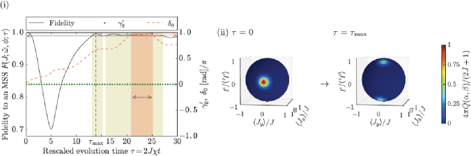
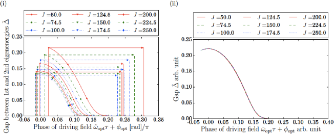
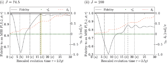
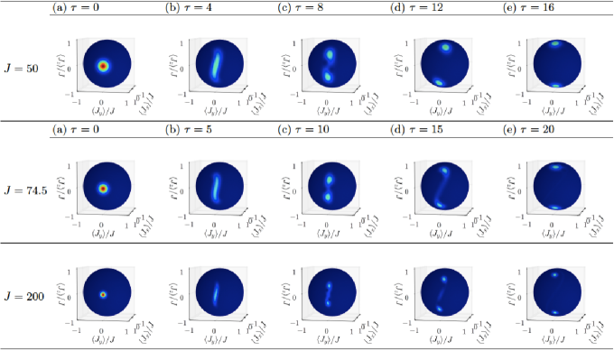
where is numerically maximised with respect to , , and by the basin-hopping method basin ; Wales . The fidelity in in Eq. (6) for fixed and has a local maximum at the rescaled elapsed time as shown in Fig. 1 (i). At , the Q-function becomes a superposition of two CSSs as shown in Figs. 1 (ii). We numerically obtain and the fidelity of the first local maximum . After , the state maintains high fidelity for quite a while as shown in Fig. 1 (i), which implies that the fidelity is rather insensitive to timing in creating an MSS via this method (see also Appendix B and Figs. 9). We also note that is time-independent during the time evolution given by Eq. (1) as shown in Fig. 1 (i), which implies that the phase between and is preserved under the Hamiltonian in Eq. (1).
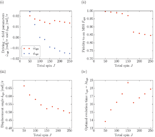
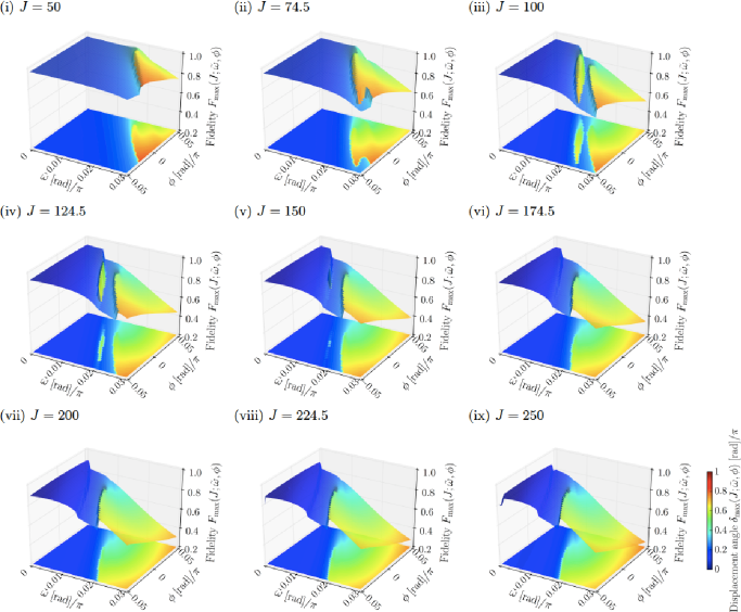
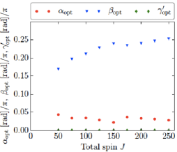
Next, in order to investigate the driving frequency and its phase optimising the fidelity and the displacement angle at , we plot and displacement angle with respect to and for in Appendix B. We estimate and maximising under the condition and plot , , , , and against the total spin in Figs. 2. The maximum fidelity jumps in the regime , which is caused by a finite probability distribution around and at as shown in the Q-functions in Figs. 10 of Appendix B.
III Nonclassicality Witness and Precision Measurements
To witness the nonclassicality of the generated MSS in experiments, we measure the parity of the spins in the direction, after rotating along the axis by a small angle , which is the same protocol as the Heisenberg-limited measurement using maximally entangled states Bollinger1 . If the state is a perfect MSS, i.e., , the quantum fluctuation in the parity, , exhibits fringes with respect to as
| (8) |
whose derivation is detailed in Appendix C. On the other hand, when the state is a mixed state of two CSSs, , i.e., no fringe can be observed as shown in Appendix C.
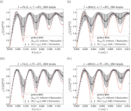
We compare the fringes produced by perfect MSSs, MSSs without spin number fluctuations, with Gaussian number fluctuations of spins, and with uniform fluctuations in the driving field magnitude , where for and as shown in Figs 3. In the cold-atom experiments, the number fluctuations and the fluctuations in due to magnetic-field fluctuations may fluctuate respectively by Strobel and a few percent at least, and they are the major noise sources that degrade fringe visibility, while the preparation time , the driving frequency , and the driving phase can be controlled precisely enough. We also numerically show robustness of fringes against the nonlinear interaction energy , which is equivalent to robustness against , in Appendix C. Figures 3 imply that the major noise source is the number fluctuation rather than the driving-field fluctuation; nonetheless we still can expect to observe the nonclassicality of the state even with fluctuations in the number of spins as shown in Figs. 13 of Appendix C.
The other major noise source would be the magnetic field in the direction. The magnetic field gives rise to a linear Zeeman term in the Hamiltonian in Eq. (1), where the linear Zeeman energy with the Landé -factor and the Bohr magneton . The term harms the preservation of the relative phases ’s between the two eigenstates during the time evolution. The linear Zeeman energy can be well controlled in experiments when the driving field is switched off; however, once it is turned on, it may be an experimentally challenging to cancel the linear Zeeman energy. The analysis of the effects of the linear Zeeman energy and its fluctuation and how it can be circumvented are left as future problems.
In addition to these noises, to detect the interferometric characteristics, we typically measure the spin parity in the direction in the single-spin resolution. In such a scenario, trapped ion systems have a clear advantage over BECs.
The states created via our method can also be applied to precision measurements of the rotation angle around the axis. Let us consider a frequency measurement of fringes given by in Eq. (8). If a perfect MSS is created, the spectrum of the fringes are given by
| (9) |
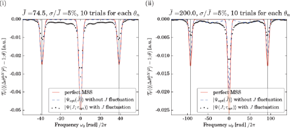
where is the frequency, the standard variation , and the mean value . In reality, however, a deterioration in the fidelity and spin-number fluctuations cannot be ignored, and they might wipe out the spectrum. We numerically calculate the spectra for the optimized state without spin-number fluctuations and the state with Gaussian number fluctuations of spins for spins and spins. Here, we assume that the states are rotated by , where and such that is the maximum integer satisfying . For each , we perform ten rotation-and-measurement procedures and the number of spins varies according to the normal distribution thoughout the procedures. The mean values of are discrete-Fourier-transformed to obtain spectra, which are shown in Figs. 4. The discrete Fourier transform is defined as
| (10) |
which relates to Eq. (9) as
| (11) |
In Figs. 4, we plot of the optimized states without spin-number fluctuations and the states with Gaussian number fluctuations of spins and compare them with those of the ideal MSSs given in Eq. (9). When the number of spins is relatively small, i.e., , the state is almost a perfect MSS in the case without a spin-number fluctuations, and we can expect to observe clear dips at . When the number of spins increases to be , the decrease in fidelity makes the dips shallower; however, they are still clearly seen. The Gaussian number fluctuations of spins halve the depth of dips, while their positions remain almost unchanged, which indicates that the states created via our method can be applied to probes of precision measurements and sensing.
IV Discussion and Conclusion
Finally we evaluate the time to generate a MSS state and compare the generation time with the coherence times reported in Refs. Strobel ; Bohnet . First, we consider the case of the two-level system consisting of spin up and down states of 9Be+ ions in a two-dimensional triangular lattice Bohnet . The interaction energy and the coherence time are respectively estimated to be and for ions. Here, the major source of decoherence is spontaneous emission from an off-resonant laser beam creating uniform - coupling between spins. For spins, we can estimate the generation time for an MSS to be , which is two order of magnitude shorter than that for the OAT interaction given by and sufficiently smaller than the coherence time.
Next, we consider the two-level system consisting of and of cold 87Rb atoms Strobel . The major source of decoherence is the atom-number decay caused by the decay of the state, inelastic scattering, and three-body recombination. The interaction energy and the coherence time are respectively assumed to be and for atoms, whereas the coherence time for 500 spins can be estimated as [ms]. In this case, the coherence time is comparable to the MSS evolution time, which is again two order of magnitude faster than the evolution time to obtain an MSS via the OAT interaction. A stronger interaction between atoms could make a cold atom system to be a better candidate which shortens the MSS creation time.
The speedup on the MSS generation time tends to be more prominent when the ensemble size gets larger, and it can be a significant advantage of this scheme to experimentally generate and test these states. These numbers are promising for relatively large spin ensembles to form a MSS with the current technology.
ACKNOWLEDGMENTS
The authors would thank Shane Dooley, Takeshi Fukuhara, Michael Hanks, C. A. Holmes, Seth Lloyd, William J. Munro, Nguyen Thanh Phuc, Yoshiro Takahashi, and Masahito Ueda. This work is supported by MEXT Grant-in-Aid for Scientific Research on Innovative Areas KAKENHI Grant Number JP15H05870, MEXT Grant-in-Aid for Scientific Research(S) KAKENHI Grant Number JP25220601, and CREST, Japan Science and Technology Agency.
Appendix A Mechanism of Macroscopic-superposition-state Creation
We discuss the time evolution of by the rescaled Hamiltonian to obtain the optimum MSS given by
| (12) |
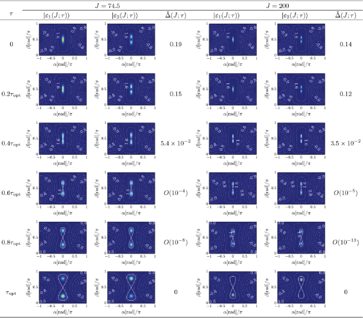
from to at which is created. Here, we define the highest energy eigenstate and the second-highest energy eigenstate of as and with the eigenenvalues and , respectively. We plot the gap between and in Figs. 5 and the Q-functions of these two eigenstates in Figs. 6. The gap closes at a certain and the two highest eigenstates and become states similar to two coherent spin states (CSSs) and the phase between them cannot be determined.
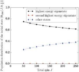
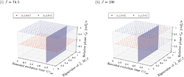
The initial state follows until the gap closes, since the initial state, i.e., , has relatively high population on , whereas it does not populate on as shown in Fig. 7. In such time evolution under a gap-closing Hamiltonian, in general, the state becomes a mixed state of the highest and the second highest energy eigenstates after the gap closes, because the phase between these two states cannot be determined. In the case of the time evolution by , however, the generated state is robust against the phase uncertainty. The reason can be explained as follows: The relative phases between of both the initial state and before the gap closes are , while ’s of are as shown in Fig. 8. The Hamiltonian preserves for all , since after an infinitesimally small time evolution by under , the phases of a state become
| (13) | |||
| (14) |
so the phase between and is preserved. Therefore, after the gap closes, the state becomes the superposition state of and so that regardless of the value of the number of spin and other parameters in the Hamiltonian in Eq. (1), and we can expect creation of an MSS via the Hamiltonian in Eq. (1) even though the gap between the highest and the second highest energy eigenstates closes during the time evolution.
Appendix B MSS generation via the Hamiltonian in Eq. (1) and parameter optimization
B.1 Time dependence of fidelity, relative phase, and displacement angle
Starting from the initial state , the state evolves under the Hamiltonian in Eq. (1) and an MSS is formed. We plot the fidelity , the relative phase , and the displacement angle , which are respectively defined in Eqs. (5), (6), and (4), as functions of the rescaled evolution time for , , and in Figs. 9. Here, in order to obtain , , and , the probability is numerically maximized with respect to , , and by the basin-hopping method basin , which finds the global minimum or maximum of a smooth scalar function with one or more variables Wales . The first local maximum of the fidelity and its corresponding evolution time are obtained from in Figs. 9 by the brute-force search that starts from in the temporal order. The obtained ’s are indicated by the black and thin dashed lines in Figs. 9.
In order to visually display the MSS creation, we plot the Q-functions of at ’s indicated by the black and thin dotted lines (a)-(e) of Figs. 9 in Figs. 10. As shown in Figs. 9, at the beginning of the time evolution, the fidelity decreases, while the displacement angle increases. In this process, the state is squeezed, which are illustrated in the Q-functions in Figs. 10 (b). After that, the Q-function on the Bloch sphere is bent and tore off at and as we can see in Figs 10 (b)-(c), and the two peaks of the Q-function move in the opposite directions as shown in Figs. 10 (c)-(e). For and , finite portions of the probability distribution remain around and , which causes a decrease in the fidelity of the first local maximum.
B.2 Driving frequency and phase dependence of fidelity and displacement angle
We optimize the frequency and the phase of the driving field with respect to the fidelity and the displacement angle and obtain the dependences of the optimized fidelity , the displacement angle , their corresponding driving-field parameters and , and the evolution time . Here, the displacement angle is calculated from and . We plot and as functions of and in Figs. 11 for - and obtain and by the brute-force search such that is the maximum of with respect to and in the parameter region satisfying . Figures 11 are plotted against pairs of and and we do finer calculation with the precision of and around the peaks obtained from Figs. 11 in order to estimate and for . The dependence of , , and are shown in Fig. 12. The plot of indicates that the MSS creation via the Hamiltonian in Eq. (1) is robust against the fluctuations in the spin number, the driving-field frequency, and the evolution time.
Appendix C Interferometry using MSSs
C.1 Idealistic case
Suppose we can prepare a perfect MSS given by Eq. (2). The nonclassicality of the MSS can be observed by the following procedure Bollinger1 : First, let an MSS rotate about the axis by a small angle , which results in the state , i.e.,
| (15) |
Then, measure the parity of of the spin ensemble:
| (16) |
where is given in Eq. (4) and we neglect the terms proportional to on the right-hand side of the last equality, since it is as small as in the parameter region of and that satisfies for - as we plot in Fig. 12. The parameter region also verifies another important approximation: The sum on the right-hand side of Eq. (16) can be well approximated by the Gaussian integral, since the term in Eq. (16) can be considered as the binomial distribution of the number of success in a sequence of independent trials with the success rate of and the absolute value of its skewness is approximately given by
| (17) |
which indicates this binomial distribution can be well approximated by the normal distribution. Therefore, the expectation value of the parity of is approximately obtained as
| (18) |
and the variance of the parity of is given by
| (19) |
Equation (19) implies that one can expect to observe the fringe for the rotation angle satisfying . This range of the rotation angle allows us to observe about fringes for , which implies that we can expect to observe four fringes for a spin ensemble and seven fringes for a spin ensemble if a perfect MSS can be prepared. We also note that the width of the single fringe is given by
| (20) |
for , which implies that an MSS can be utilized as a probe of Heisenberg-limited spectroscopy. On the other hand, when the state is mixed, i.e.,
| (21) |
the variance of the parity of after the rotation about the axis by an angle is given by
| (22) |
and no fringes can be observed.
C.2 MSSs with spin number fluctuations
As shown in Eq. (19) in the previous subsection, a perfect MSS manifests fringes of whose width is given by the Heisenberg-limit scaling law . The fringes generated by ; however, are expected to be degraded by the imperfection of . Moreover, the number of spins in an ensemble may well have finite fluctuation in experiments, for instance, the number of atoms is fluctuating as in Ref. Strobel , and the fringes may fade away, depending on the magnitude of the number fluctuations. In order to investigate the robustness of the fringes generated by against the imperfection of the fidelity to the perfect MSS and the spin-number fluctuation, we numerically calculate the fringes of generated by whose spin number is Gaussian-fluctuating, i.e., the probability to have spins can be expressed as the normal distribution with the mean value of and the standard deviation given by
| (23) |
In the case of Ref. Strobel , the mean and the standard deviation of the spin number are given by and , respectively. In our calculation of with finite spin-number fluctuation, 250 pseudo-random spin numbers with the probability density given by Eq. (23) are generated by the Mersenne Twister method so that the difference between the mean spin number of traials and in Eq. (23) and their respective standard deviations and satisfy and .
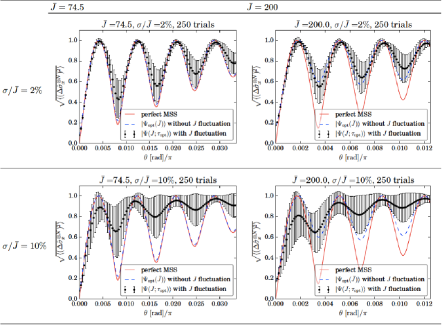
We show the fringes for and without and with the spin-number fluctuations of and in Figs. 13. The fringes for the perfect MSS and without the spin-number fluctuation almost coincide with each other in the case of , when the fidelity to the perfect MSS exceeds 0.99. On the other hand, the magnitudes of the fringes generated by decrease in comparison with the perfect MSS even without the spin-number fluctuation in the case of , when the fidelity to the perfect MSS degraded to be ; however, the magnitude of the fringe created by is diminished more slowly than the perfect MSS with respect to the rotation angle and the positions of the fringe peaks does not change from those of the perfect MSS. Thus we can expect to observe the fringes and make use of it to estimate the rotation angle up to the spin number of at least when the number of spins can be deterministically prepared. Figure 13 also imply the robustness against the spin-number fluctuation of . The fringes with the spin number fluctuation of is not suitable for the rotation-angle measurement; however, they still manifest the nonclassicality, since we can clearly see the region on either side of the first peak of at given in Eq. (20) as shown in Figs. 13.
C.3 Other noise sources
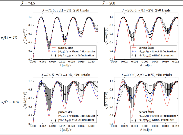
The other major noise sources are the fluctuations in the magnitude of the driving field and the evolution time of an MSS creation during a series of trials to obtain fringes. Here, is well controllable to within the order of as well as driving-field parameters and whose fluctuations are negligible when the interaction strength is given by ; however, it can be a major source of fluctuations when the achievable interaction strength gets larger to be .
The fluctuation in can be caused by the fluctuation in the energy splitting between two internal degrees of freedom comprising a pseudo spin. We assume that uniformly distributes between and simulate the fringes produced by with the fluctuation in of and for and as shown in Figs. 14. Here, we generate 250 pseudo-random value of ’s, each of which are un-correlated, and ensure that the average of of the 250 trials, , satisfies . We can observe the fringes even when fluctuates of its mean value.
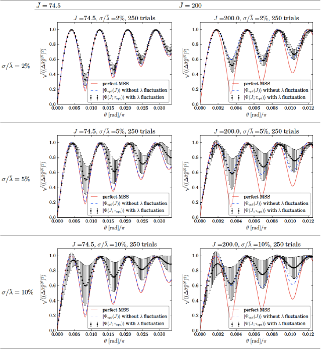
The fluctuation in is equivalent to the fluctuation in the nonlinear interaction energy . So, we assume that has a uniform distribution between and obtain the fringes of produced by the MSSs with random for and and for , , and . As in the case of fluctuating , we can expect to observe interference fringes when or fluctuates of its magnitude.
References
- (1) George C. Knee, Kosuke Kakuyanagi, Mao-Chuang Yeh, Yuichiro Matsuzaki, Hiraku Toida, Hiroshi Yamaguchi, Shiro Saito, Anthony J. Leggett, and William J. Munro, Nature Comm, 7, 13253 (2016).
- (2) Horace P. Yuen, Phys. Rev. A 13, pp. 2226-2243 (1976).
- (3) Hwang Lee, Pieter Kok, and Jonathan P. Dowling, J. Mod. Opt. 49, pp. 2325-2338 (2002); Jonathan P. Dowling, Contemporary Phys. 49, pp. 125-143 (2008).
- (4) Klaus Mølmer and Andres Sørensen, Phys. Rev. Lett. 82, pp. 1835-1838 (1999); Andres Sørensen and Klaus Mølmer, Phys. Rev. A 62, 022311 (2000).
- (5) G. J. Milburn, arXiv:9908037 [quant-ph] (1999).
- (6) D. D. Bhaktavatsala Rao, Nir Bar-Gill, and Gershon Kurizki, Phys. Rev. Lett. 106, 010404 (2011).
- (7) N. D. Mermin, Phys. Rev. Lett. 65, pp. 1838-1840 (1990).
- (8) J. J . Bollinger, Wayne M. Itano, D. J. Wineland, and D. J. Heinzen, Phys. Rev. A 54, pp. R4649-R4652 (1996).
- (9) Christopher C. Gerry and Rainer Grobe, J. Mod. Opt. 44, pp. 44-53 (1997).
- (10) S. F. Huelga, C. Macchiavello, T. Pellizzari, A. K. Ekert, M. B. Plenio, and J. I. Cirac, Phys. Rev. Lett. 79, pp. 3865-3868 (1997).
- (11) Agedi N. Boto, Pieter Kok, Daniel S. Abrams, Samuel L. Braunstein, Colin P. Williams, and Jonathan P. Dowling, Phys. Rev. Lett. 85 pp. 2733-2736 (2000).
- (12) M. W. Mitchell, J. S. Lundeen, and A. M. Steinberg, Nature 429, pp. 161-164 (2004).
- (13) D. Leibfried, M. D. Barrett, T. Schaetz, J. Britton, J. Chiaverini, W. M. Itano, J. D. Jost, C. Langer, D. J. Wineland, Science 304, pp. 1476-1478 (2004)
- (14) Vittorio Giovannetti, Seth Lloyd, Lorenzo Maccone, Science 306, pp. 1330-1336 (2004).
- (15) Luca Pezzé and Augusto Smerzi, Phys. Rev. Lett. 102, 100401 (2009).
- (16) Jonathan A. Jones, Steven D. Karlen, Joseph Fitzsimons, Arzhang Ardavan, Simon C. Benjamin, G. Andrew D. Briggs, John J. L. Morton, Science 324, pp. 1166-1168 (2009); Stephanie Simmons, Jonathan A. Jones, Steven D. Karlen, Arzhang Ardavan, and John J. L. Morton, Phys. Rev. A 82, 022330 (2010).
- (17) Robert McConnell, Hao Zhang, Senka Ćuk, Jiazhong Hu, Monika H. Schleier-Smith, and Vladan Vuletić, Phys. Rev. A 88, 063802 (2013).
- (18) T. C. Ralph, A. Gilchrist, G. J. Milburn, W. J. Munro, and S. Glancy, Phys. Rev. A 68, 042319 (2003).
- (19) Sean D Barrett, Peter P Rohde, and Thomas M Stace, New J. Phys. 12 093032 (2010).
- (20) Petr Marek and Jaromír Fiurášek, Phys. Rev. A 82, 014304 (2010).
- (21) L.-M. Duan, M. D. Lukin, J. I. Cirac, and P. Zoller, Nature 414, pp. 413-418 (2001).
- (22) F. T. Arecchi, Eric Courtens, Robert Gilmore, and Harry Thomas, Phys. Rev. A 6, pp. 2211-2237 (1972).
- (23) G. S. Agarwal, R. R. Puri, and R. P. Singh, Phys. Rev. A 56, pp. 2249-2254 (1997).
- (24) Sergey M. Chumakov, Alejandro Frank, and Kurt Bernardo Wolf, Phys. Rev. A 60, pp. 1817-1823 (1999).
- (25) Jan Benhelm, Gerhard Kirchmair, Christian F. Roos, and Rainer Blatt, Nature Phys. 4 pp. 463-466 (2008).
- (26) A. Voje, J. M. Kinaret, and A. Isacsson, Phys. Rev. B 85 205415 (2012).
- (27) Tomás̃ Opatrný and Klaus Mølmer, Phys. Rev. A 86 023845 (2012).
- (28) Shane Dooley and Timothy P. Spiller, Phys. Rev. A 90 012320 (2014).
- (29) Hon Wai Lau, Zachary Dutton, Tian Wang, and Christoph Simon, Phys. Rev. Lett. 113 090401 (2014).
- (30) Christopher C. Gerry and Rainer Grobe, Phys. Rev. A 56, pp. 2390-2396 (1997); ibid. 57, pp. 2247-2250 (1998).
- (31) José Recamier, Octavio Castanõs, Rocio Jáuregui and Alejandro Frank, Phys. Rev. A 61 063808 (2000).
- (32) S. D. Bennett, N. Y. Yao, J. Otterbach, P. Zoller, P. Rabl, and M. D. Lukin, Phys. Rev. Lett. 110, 156402 (2013).
- (33) Shane Dooley, Emi Yukawa, Yuichiro Matsuzaki, George C. Knee, William J. Munro, and Kae Nemoto, New J. Phys. 18, 053011 (2016).
- (34) Wei-Bo Gao, Chao-Yang Lu, Xing-Can Yao, Ping Xu, Otfried Gühne, Alexander Goebel, Yu-Ao Chen, Cheng-Zhi Peng, Zeng-Bing Chen, and Jian-Wei Pan, Nature Phys. 6, pp. 331-335 (2010).
- (35) Pieter Kok, Hwang Lee, and Jonathan P. Dowling, Phys. Rev. A 65, 052104 (2002).
- (36) Anne E. B. Nielsen and Klaus Mølmer, Phys. Rev. A 75, 063803 (2007).
- (37) Yu-Ao Chen, Xiao-Hui Bao, Zhen-Sheng Yuan, Shuai Chen, Bo Zhao, and Jian-Wei Pan, Phys. Rev. Lett. 104, 043601 (2010).
- (38) Ryotaro Inoue, Shin-Ichi-Ro Tanaka, Ryo Namiki, Takahiro Sagawa, and Yoshiro Takahashi, Phys. Rev. Lett. 110, 163602 (2013).
- (39) Navin Khaneja, Roger Brockett, and Steffen J. Glaser, Phys. Rev. A 63, 032308 (2001); Navin Khaneja and Steffen J. Glaser, Chem. Phys. 267, pp. 11-23 (2001).
- (40) Jun Zhang, Jiri Vala, Shankar Sastry, and K. B. Whaley, Phys. Rev. A 67, 042313 (2003); Jun Zhang and K. B. Whaley, Phys. Rev. A 71, 052317 (2005).
- (41) M. Kitagawa and M. Ueda, Phys. Rev. A 47, pp. 5138-5143 (1993).
- (42) J. Estève, C. Gross, A. Weller, S. Giovanazzi, and M. K. Oberthaler, Nature 455, pp. 1216-1219 (2008); C. Gross, T. Zibold, E. Nicklas, J. Estève, and M. K. Oberthaler, Nature 464, pp. 1165-1169 (2010).
- (43) Ian D. Leroux, Monika H. Schleier-Smith, and Vladan Vuletić, Phys. Rev. Lett. 104, 073602 (2010); Monika H. Schleier-Smith, Ian D. Leroux, and Vladan Vuletić, Phys. Rev. A 81, 021804(R) (2010).
- (44) Max F. Riedel, Pascal Böhi, Yun Li, Theodor W. Hänsch, Alice Sinatra and Philipp Treutlein, Nature 464, pp. 1170-1173 (2010).
- (45) Helmut Strobel, Wolfgang Muessel, Daniel Linnemann, Tilman Zibold, David B. Hume, Luca Pezzè, Augusto Smerzi, and Markus K. Oberthaler, Science 345, pp. 424-427 (2014).
- (46) Justin G. Bohnet, Brian C. Sawyer, Joseph W. Britton, Michael L. Wall, Ana Maria Rey, Michael Foss-Feig, and John J. Bollinger, Science 352, pp. 1297-1301 (2016).
- (47) C. A. Sackett, D. Kielpinski, B. E. King, C. Langer, V. Meyer, C. J. Myatt, M. Rowe, Q. A. Turchette, W. M. Itano, D. J. Wineland and C. Monroe, Nature 404, pp. 256-259 (2000); D. Leibfried, E. Knill, S. Seidelin, J. Britton, R. B. Blakestad, J. Chiaverini, D. B. Hume, W. M. Itano, J. D. Jost, C. Langer, R. Ozeri, R. Reichle and D. J. Wineland, Nature 438, pp. 639-642 (2005).
- (48) Thomas Monz, Philipp Schindler, Julio T. Barreiro, Michael Chwalla, Daniel Nigg, William A. Coish, Maximilian Harlander, Wolfgang Hänsel, Markus Hennrich, and Rainer Blatt, Phys. Rev. Lett. 106, 130506 (2011).
- (49) Yun Li, P. Treutlein, J. Reichel, and A. Sinatra, Eur. Phys. J. B 68, pp. 365-381 (2009).
- (50) J. I. Cirac, M. Lewenstein, K. Mølmer, and P. Zoller, Phys. Rev. A 57, pp. 1208-1218 (1998).
- (51) D. Gordon and C. M. Savage, Phys. Rev. A 59, pp. 4623-4629 (1999).
- (52) A. Micheli, D. Jaksch, J. I. Cirac, and P. Zoller, Phys. Rev. A 67, 013607 (2003).
- (53) H. J. Lipkin, N. Meshkov, and J. Glick, Nucl. Phys. 62, pp. 188-198 (1965).
- (54) W. Muessel, H. Strobel, D. Linnemann, T. Zibold, B. Juliá–Díaz, and M. K. Oberthaler, Phys. Rev. A 92, 023603 (2015).
- (55) S. Chaudhury, A. Smith, B. E. Anderson, S. Ghose, and P. S. Jessen, Nature 461, pp. 768-771 (2009).
- (56) https://docs.scipy.org/doc/scipy/reference/generated/scipy.optimize.basinhopping.html
- (57) D. J. Wales and J. P. K. Doye, Journal of Physical Chemistry A 101, pp. 5111-5116 (1997).