Cavity assisted single- and two-mode spin-squeezed states via phase-locked atom-photon coupling

Abstract

We propose a scheme to realize the two-axis counter-twisting spin-squeezing Hamiltonian inside an optical cavity with the aid of phase-locked atom-photon coupling. By careful analysis and extensive simulation, we demonstrate that our scheme is robust against dissipation caused by cavity loss and atomic spontaneous emission, and it can achieve significantly higher squeezing than one-axis twisting. We further show how our idea can be extended to generate two-mode spin-squeezed states in two coupled cavities. Due to its easy implementation and high tunability, our scheme is experimentally realizable with current technologies.

Introduction. – Since the early work of Kitagawa and UedaUeda and others JianMa ; Wineland , spin-squeezed states have attracted much interest due to their close relations with quantum information processing Inform1 ; Inform2 ; Helmerson ; Micheli ; Lee ; Riedel and precision metrology Ueda ; JianMa ; Metro1 ; Metro2 ; Metro3 . In the original work of Kitagawa and UedaUeda , two mechanisms, namely one-axis twisting (OAT) and two-axis counter-twisting (TACT), were proposed to generate spin-squeezed states. Preparation of such novel states has been the subject of many studies in various physical setups such as feedback systemsThomsen , Bose-Einstein condensates (BEC) Riedel ; Metro3 ; OATe1 ; OATe2 ; OATe3 ; TATt1 ; TATt2 ; TATt3 ; TATt4 ; Toroidal , Rydberg lattice clocks Gil , and atomic systems in cavities CavAtom1 ; CavAtom2 ; CavAtom3 ; CavAtom4 ; CavAtom5 ; Twocavities ; CavAtom6 . To the best of our knowledge, all experiments to date focus on OAT spin-squeezing, whereas TACT spin-squeezed states have not been realized in experiments yet.

In quantum metrology, it is theoretically demonstrated Ueda ; JianMa that TACT states are fundamentally superior to OAT states because measurement systems based on them can approach the Heisenberg limit in which the precision of the measurement scales with $1/N$, $N$ being the number of particles in the system. In contrast, the precision allowed by OAT states scales with $1/N^{2/3}$. Hence, it remains a very important task to generate and exploit TACT spin-squeezed states using methods and techniques within the reach of current technologies. There have been a few theoretical proposals such as converting OAT into effective TACT TATt1 ; TATt2 ; TATt3 , implementing TACT with molecular states Helmerson ; TATt4 , utilizing ultracold atoms in two cavities Twocavities , employing feedbacks in the measurement system Thomsen , and using toroidal BECs Toroidal . Nevertheless, due to the demanding experimental requirements of these schemes, it remains experimentally challenging to generate TACT spin-squeezed states.

In this work, we propose a scheme to realize a TACT Hamiltonian in a cavity-atom system. Our proposal relies on phase-locked coupling between atoms and photons only. Since both the atoms and cavity modes are only virtually excited, it has the important advantage of being largely immune to atomic and cavity dissipation. Further, our scheme can be easily generalized to generate two-mode spin-squeezed (TMSS) states by coupling two cavities, which can be used to estimate two observables simultaneously even when they do not commute. They are widely used in many quantum applications such as entanglement demonstration TMSS1 ; TMSS3 , quantum teleportation TMSSqt , and quantum metrology TMSSqm . Considering the rapid advance in cavity technology including the availability of high-finesse optical cavities and strong cavity-atom coupling Cavity1 ; Cavity2 ; Cavity3 ; Cavity4 ; Cavity5 ; Cavity6 ; Cavity7 , our proposal can be realized with no fundamental difficulty.

Effective Hamiltonian. – We start by considering an ensemble of $N$ four-level atoms in an optical cavity coupled to a single cavity mode and external laser fields. The explicit level configuration is illustrated in Fig.1, where $g_{1}$ and $g_{2}$ are the cavity-atom coupling strengths driving the atomic transitions $|1\rangle\leftrightarrow|3\rangle$ and $|2\rangle\leftrightarrow|4\rangle$, $\widetilde{\Omega}_{1,2}$ and $\Omega_{1,2}$ are Rabi frequencies of the external laser fields, and $\Delta_{1,2}$, $\delta_{1,2}$ and $\gamma_{1,2}$ are detunings. To realize the desired TACT interaction, we also assume a fixed relative phase of $\pi/2$ ($-\pi/2$) between $\Omega_{1}$($\Omega_{2}$) and $\widetilde{\Omega}_{1}$($\widetilde{\Omega}_{2}$) Cho ; Chen . The Hamiltonian reads

$$H = \sum^{N}_{j=1}\big{\{}\frac{e^{i\varphi}}{2}\left[\widetilde{\Omega}_{2}e^{-i(\Delta_{2}+\delta_{2})t}-i\Omega_{2}e^{-i(\Delta_{2}-\gamma_{2})t}\right]|1\rangle_{j}\langle 4|$$ (1)

$$+ \frac{e^{-i\varphi}}{2}\left[\widetilde{\Omega}_{1}e^{-i(\Delta_{1}+\delta_{1})t}+i\Omega_{1}e^{-i(\Delta_{1}-\gamma_{1})t}\right]|2\rangle_{j}\langle 3|$$

$$+ g_{1}|1\rangle_{j}\langle 3|a^{\dagger}e^{-i\Delta_{1}t}+g_{2}|2\rangle_{j}\langle 4|a^{\dagger}e^{-i\Delta_{2}t}+h.c.\big{\}},$$

where $a^{\dagger}$($a$) is the creation (annihilation) operator of the cavity mode, $\pm\varphi$ and $\pm(\varphi-\frac{\pi}{2})$ are the phases of the external laser fields, and the detunings are defined as $\Delta_{1(2)}=\omega_{3(4)}-\omega_{1(2)}-\omega_{c}$, $\gamma_{1(2)}=\omega_{2(1)}-\omega_{1(2)}-\omega_{c}+\omega_{L_{1}(L_{2})}$, and $\delta_{1(2)}=\omega_{1(2)}-\omega_{2(1)}+\omega_{c}-\omega_{\widetilde{L}_{1}(\widetilde{L}_{2})}$ with $\omega_{L_{1,2},\widetilde{L}_{1,2}}$ and $\omega_{c}$ being the frequencies of the driving lasers and the cavity mode. The rotating wave approximation was used to derive the Hamiltonian in Eq.(1) in the rotating frame defined by $H_{0}=\sum^{N}_{j=1}\sum^{4}_{k=1}\omega_{k}|k\rangle_{j}\langle k|+\omega_{c}(a^{\dagger}a+\frac{1}{2})$. To simplify our discussion, here and in the following, we assume $\delta=\delta_{1}=\delta_{2}$, $\gamma=\gamma_{1}=\gamma_{2}$, and set $\varphi=0$.

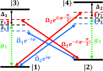
Figure 1: (Color online) Atomic energy levels and transitions between them. The complex Rabi frequencies $\widetilde{\Omega}_{1}e^{-i\varphi}$, $\widetilde{\Omega}_{2}e^{i\varphi},\Omega_{1}e^{-i(\varphi-\frac{\pi}{2})}$, and $\Omega_{2}e^{i(\varphi-\frac{\pi}{2})}$ are associated with four phase-locked driving lasers. $g_{1,2}$ is the coupling strength between the atom and the cavity mode. $\Delta_{1,2}$, $\delta_{1,2}$ and $\gamma_{1,2}$ are detunings.

For large detunings with

$$|\Delta_{1,2}|,|\Delta_{1,2}+\delta|,|\Delta_{1,2}-\gamma|\gg|g_{1,2}|,|\Omega_{1,2}|,|\widetilde{\Omega}_{1,2}|,$$ (2)

all the high energy levels can be adiabatically eliminated, leading to the following effective Hamiltonian involving only the two lowest states and the cavity mode,

$$H^{\prime} = \left\{c_{z}-c^{\prime}_{z}\sin\big{[}(\delta+\gamma)t\big{]}\right\}S_{z}$$ (3)

$$- \big{[}\frac{A}{2}S_{x}a^{\dagger}e^{i\delta t}+\frac{B}{2}S_{y}a^{\dagger}e^{-i\gamma t}+h.c.\big{]}.$$

Here the collective atomic spin operators are defined as $S_{z}=\frac{1}{2}\sum^{N}_{j=1}(|1\rangle_{j}\langle 1|-|2\rangle_{j}\langle 2|)$, $S_{x}=\frac{1}{2}\sum^{N}_{j=1}(|1\rangle_{j}\langle 2|+|2\rangle_{j}\langle 1|)$, and $S_{y}=\frac{i}{2}\sum^{N}_{j=1}(|2\rangle_{j}\langle 1|-|1\rangle_{j}\langle 2|)$. The explicit expressions for the coefficients $c_{z}$, $c_{z}^{\prime}$, $A$, and $B$ can be found in the Supplementary Material SM .

If we further assume that the effective couplings in Eq.(3) are much weaker than the detunings, i.e.,

$$|\delta|,\ |\gamma|,\ |\delta\pm\gamma|\gg N|A|/4,\ N|B|/4,$$ (4)

the cavity mode is virtually excited only and can be adiabatically eliminated too. We then obtain the following effective Hamiltonian

$$H_{eff}=c_{z}S_{z}-c_{x}S^{2}_{x}+c_{y}S^{2}_{y}$$ (5)

with $c_{x}=\frac{A^{2}}{4\delta}$ and $c_{y}=\frac{B^{2}}{4\gamma}$ SM . This is the celebrated Lipkin-Meshkov-Glick (LMG) model JianMa . When $c_{z}=0$ and $c_{x}=c_{y}=\chi$, it reduces to the standard TACT Hamiltonian in Ueda . Experimentally, all coefficients $c_{x,y,z}$ can be controlled by adjusting the Rabi frequencies of the driving lasers. If necessary, $c_{z}$ can also be compensated by an external magnetic field Duan .

To characterize the degree of spin-squeezing, we introduce the parameter Ueda ; JianMa

$$\xi^{2}=\frac{(\Delta S_{\perp})^{2}_{min}}{S/2}.$$ (6)

Here $S=N/2$ with ${\bf S}=(S_{x},\ S_{y},\ S_{z})$ the total spin operator, and $(\Delta S_{\perp})^{2}_{min}=(\langle{\bf S}^{2}_{\perp}\rangle-\langle{\bf S}_{\perp}\rangle^{2})_{min}$ is the minimum spin fluctuation in the direction perpendicular to the average spin $\langle{\bf S}\rangle$. A state is a spin coherent state (spin-squeezed state) if $\xi^{2}=1$ ($\xi^{2}<1$) Ueda .

Numerical Simulation. – In order to check the validity of our approximations, we numerically simulate the system evolution under the effective Hamiltonian in Eq.(5) and the original Hamiltonian in Eq.(1) and compare the results. To fulfill the approximations, the explicit parameters are chosen as follows: $g_{1,2}=\Omega_{1,2}=\widetilde{\Omega}_{1,2}=\Omega=5\times 10^{7}s^{-1}$ , $\Delta_{1,2}=\Delta=10^{9}s^{-1}$, $\delta_{1,2}=10^{8}s^{-1}$, $\gamma_{1,2}=1.26\times 10^{8}s^{-1}$. With these parameters, the effective model reduces to a standard TACT Hamiltonian with $c_{z}=0$ and $\chi=5.69\times 10^{4}s^{-1}$. We also assume that initially the cavity is in the vacuum state and the atoms are all in the state $|1\rangle$, which corresponds to a coherent spin state in the $z$ direction.

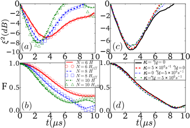
Figure 2: (Color online) (a,b) Time evolution of $\xi^{2}$ and $F$ with $H$ in Eq.(1) and $H_{eff}$ in Eq.(5) without dissipation for $N=6$, $8$, and $10$. (c,d) Time evolution of $\xi^{2}$ and $F$ under the original Hamiltonian $H$ in Eq.(1) with dissipation for $N=8$.

Shown in Fig.2(a,b) are the time dependences of the squeezing parameter $\xi^{2}$ and the overlap function $F=|\langle\psi(0)|\psi(t)\rangle|$ with the initial state of the system in the ideal case without cavity leakage ($\kappa=0$) and atomic spontaneous decay ($\gamma_{d}=0$). The state evolution dictated by the effective TACT Hamiltonian in Eq.(5) agrees very well with that calculated directly from the original full Hamiltonian in Eq.(1), strong evidence that all approximations employed in our derivation are reasonable.

We note in Fig.3(b) that, though the maximum achievable squeezing (i.e. the minimum $\xi^{2}$) increases with the number of atoms $N$ JianMa ; TATt1 , the time it takes to reach it increases with $N$ too. This is because the nonlinear squeezing coefficients $c_{x}(c_{y})$ in Eq.(5) must decrease with $N$ in order to maintain the virtual excitation of the system as dictated by Eq.(4). Though virtual excitation reduces the influence of the dissipation, its eventual effect on squeezing must be carefully evaluated because of the longer squeezing time required to reach the optimal squeezing. For this purpose, we numerically solve the master equation CavAtom4 ; Master1 ; Master2 of the system

$$\frac{\partial\rho}{\partial t}=-i[H,\ \rho]-\frac{\kappa}{2}\mathcal{D}(a,\rho)-\frac{1}{2}\sum_{k=1}^{N}\sum_{s=1}^{4}\gamma_{ks}\mathcal{D}(L_{ks},\rho).$$ (7)

Here $\mathcal{D}(O,\rho)=O^{\dagger}O\rho+\rho O^{\dagger}O-2O\rho O^{\dagger}$, $\rho$ is the density matrix, $\kappa$ and $\gamma_{ks}$ are the cavity loss rate and atomic spontaneous decay rate, and $L_{k1}=|1\rangle_{k}\langle 3|$, $L_{k2}=|2\rangle_{k}\langle 3|$, $L_{k3}=|1\rangle_{k}\langle 4|$ and $L_{k4}=|2\rangle_{k}\langle 4|$ are the jump operators. The results are shown in Fig.2(c,d) for N=8. It is seen that the squeezing is robust against dissipation and the maximum achievable squeezing is only slightly influenced by cavity loss and atomic spontaneous emission as strong as $\kappa=\gamma_{d}=5\times 10^{6}s^{-1}$. Since we have confirmed the validity of the virtual excitation of the cavity mode in earlier simulations, we can adiabatically eliminate the cavity field from the full Master equation to increase the scale of our simulated system. This results in the following Master equation CavAtom4 that involves only the atomic spin degrees of freedom,

$$\begin{split}\frac{\partial\rho_{eff}}{\partial t}&=-i[H_{eff},\ \rho_{eff}]-\frac{\gamma_{d}}{2}\sum_{\alpha=z,\pm}\sum^{N}_{k=1}a_{\alpha}\mathcal{D}(\sigma^{k}_{\alpha},\rho_{eff})\\ &-\frac{\kappa}{2}\left(\frac{A^{2}}{4\delta^{2}}\mathcal{D}(S_{x},\rho_{eff})+\frac{B^{2}}{4\gamma^{2}}\mathcal{D}(S_{y},\rho_{eff})\right),\end{split}$$ (8)

where $\sigma^{k}_{z}=|1\rangle_{k}\langle 1|-|2\rangle_{k}\langle 2|$, $\sigma^{k}_{+}=|1\rangle_{k}\langle 2|$, $\sigma^{k}_{-}=|2\rangle_{k}\langle 1|$, and the explicit expressions for $a_{z,\pm}$ can be found in the Supplementary Material SM . Using Eq.(8), we can numerically simulate larger systems with more atoms. In Fig.3(a), we plot the maximum achievable squeezing in our system with strong dissipation, as well as the maximum squeezing attainable in an ideal OAT Hamiltonian with no dissipation. The results show that, even in the presence of strong dissipation, our system can achieve a higher degree of squeezing than what is possible with ideal OAT, and the advantage grows with the size of the system. In Fig.3(b), we compare the maximum achievable squeezing of an ideal TACT Hamiltonian in Eq.(5) ($c_{z}=0$) with that of ideal OAT for larger system sizes on the order of $10^{3}-10^{5}$. A large advantage is observed with our scheme. For a system size of $N=10^{5}$ atoms as in recent experiments CavAtom6 ; CavAtom7 , the ideal Hamiltonian Eq.(5) for our system can reach a squeezing of -47.4dB, significantly higher than current schemes based on OAT OATe1 ; Metro2 ; Metro3 ; Riedel ; CavAtom5 with the same system size. Since the atomic decay time, estimated as $1/\gamma_{eff}$ with $\gamma_{eff}\sim\frac{\Omega^{2}}{4\Delta^{2}}\gamma_{d}\approx\frac{\delta\chi}{g^{2}}\gamma_{d}$ CavAtom1 ; CavAtom3 ; CavAtom5 , can be longer than the time required to reach the optimal squeezing, $t_{o}=1.58lnN/(3N\chi)$ TATt1 , e.g., when $N=10^{5}$, using parameters in Fig.3(b) with $g=1.26\times 10^{7}s^{-1}$ and $\gamma_{d}=3.77\times 10^{7}s^{-1}$, the atomic decay time $1/\gamma_{eff}\approx 13ms$ is larger than $t_{o}(10^{5})\approx 2.4ms$, and the influence of cavity loss is much weaker than that of atoms’ decay as illustrated in Fig.2(c), a high degree of squeezing can be achieved.

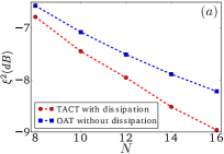
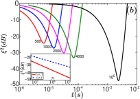
Figure 3: (Color online) (a) Comparison of the maximum achievable squeezing in our system with strong atomic and cavity dissipation rates $\kappa=\gamma_{d}=5\times 10^{6}s^{-1}$ and in a dissipation-free OAT system $H_{OAT}=\chi S_{x}^{2}$. Other parameters are the same as in Fig.2 except that $\Omega=2\times 10^{7}s^{-1}$. (b) Time evolution of $\xi^{2}$ in our system with $N=10^{3}-10^{5}$ atoms and no dissipation. Shown in the inset is the maximum achievable squeezing in our system and in OAT, both without dissipation. Relevant parameters are $\Delta_{1}=-\Delta_{2}=1.88\times 10^{10}s^{-1}$, $\gamma=2\delta=1.26\times 10^{10}s^{-1}$ and $A=B/\sqrt{2}=0.4\delta/N$ where $N=500,1000,2000,4000,$ and $10^{5}$.

Two-mode spin-squeezed states. – Our scheme can be extended to generate TMSS states TMSS1 ; TMSS3 ; TMSS2 using two cavities. Assuming a coupling between the two cavity modes, we have the following total Hamiltonian in the rotating frame,

$$H_{tc}=H_{L}+H_{R}-\widetilde{J}(a^{\dagger}_{L}a_{R}e^{i\Delta\omega t}+h.c.)$$ (9)

where $a^{\dagger}_{L,R}(a_{L,R})$ is the creation (annihilation) operator for the left and right cavity mode, $\widetilde{J}$ is the tunneling rate between the cavities, $\Delta\omega=\omega^{L}_{c}-\omega^{R}_{c}$ is the detuning between the two cavities with the local Hamiltonian $H_{\alpha\in(L,R)}=-\frac{A_{\alpha}}{2}S^{\alpha}_{x}a^{\dagger}_{\alpha}e^{i\delta_{\alpha}t}-\frac{B_{\alpha}}{2}S^{\alpha}_{y}a^{\dagger}_{\alpha}e^{-i\gamma_{\alpha}t}+h.c.$. When the coefficients and detunings satisfy the following conditions

$$\begin{split}&\delta_{L}=-\delta_{R}=\delta>0,\qquad-\gamma_{L}=\gamma_{R}=\gamma>0\\ &\Delta\omega=\delta+\gamma,\quad A_{L}=A_{R}=A,\quad B_{L}=B_{R}=B\end{split}$$ (10)

the effective Hamiltonian for the two-cavity system can then be written as SM

$$H_{T}=\chi[(S^{L}_{z})^{2}-(S^{R}_{z})^{2}]+2J\chi(S^{L}_{x}S^{R}_{y}+S^{L}_{y}S^{R}_{x})$$ (11)

with $\chi=\frac{A^{2}}{4\delta}=\frac{B^{2}}{4\gamma}$, and $J=\frac{\widetilde{J}}{\sqrt{\delta\gamma}}$. The second term in $H_{T}$ gives rise to a TMSS state. The first term, which describes the on-site nonlinear interaction in each cavity, has no contribution when $S^{L}_{z}=S^{R}_{z}$.

A TMSS state can be identified by checking that it satisfies the inequality $\Delta^{\prime}=(\Delta S^{(-)}_{x})^{2}+(\Delta S^{(+)}_{y})^{2}-\langle S^{(+)}_{z}\rangle<0$ with $S^{(\pm)}_{k}=S^{L}_{k}\pm S^{R}_{k}$ ($k=x,y,z$) TMSS1 ; TMSS2 ; TMSS3 . This criterion implies that fluctuations in nonlocal observables $S^{-}_{x}$ and $S^{+}_{y}$ can be suppressed at the same time. Thus it is possible to achieve higher measurement precisions for them simultaneously.

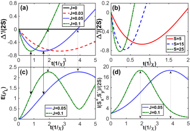
Figure 4: (Color online) Time evolution of squeezing, entanglement, and quantum fisher information of two-mode spin-squeezed states with the same total spin number for the two modes. (a) $\Delta^{\prime}$ vs $t$ while $S=N/2=5$, and $J=0,\,0.03,\,0.05,\,0.1$; (b) $\Delta^{\prime}$ vs $t$ while $J=0.1$, and $S=5,\,15,\,25$; (c) Dependence of the von Neumann entropy $E(\rho_{L})$ on time for $J=0.05,\,0.1$ when $S=5$; (d) The quantum Fisher information for $|\Psi(t)\rangle$ at $J=0.05,\,0.1$ when $S=5$.

When the total spins inside the two cavities are equal, $S_{L}=S_{R}$, a TMSS state can be obtained by letting the system evolve under $H_{T}$ from an initial state in which both cavities are in a coherent state: $|\Psi(0)\rangle=|S,S\rangle$ with $|m^{L}_{i},m^{R}_{j}\rangle$ ($m^{L,R}_{i}=-S,-S+1,\cdots,S-1,S$) the eigenvectors of $S_{z}$, and $S=N/2$ the total spin. Plotted in Fig.4(a,b) is the time evolution of $\Delta^{\prime}(t)$. One can see that $\Delta^{\prime}$ is always zero when $J=0$ as both cavities are decoupled in this case. When there is photon tunneling between the cavities and thus $J\neq 0$, $\Delta^{\prime}$ can become negative which signals the emergence of TMSS states. Comparing Fig.4(a) with Fig.4(b), we note that the time it takes to reach $\Delta^{\prime}_{min}$, the minimum value of $\Delta^{\prime}$, is controlled by the coupling strength $J$, and $\Delta^{\prime}_{min}$ decreases as $S$ increases.

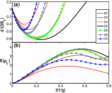
Figure 5: (Color online) Time evolution of squeezing and entanglement of two-mode spin- squeezed states with different total spin numbers for the two mode. (a) $\Delta^{\prime}$ and (b) $E(\rho_{L})$ vs $t$ for fixed $S_{L}=N_{L}/2=25$ and $J=0.1$. $S_{R}$ varies from $20$ to $30$.

To investigate the entanglement of the TMSS state, we have further calculated the von Neumann entropy $E(\rho_{L})=-\rho_{L}\ln{\rho_{L}}$ of the reduced density matrix $\rho_{L}=Tr_{R}(|\Psi\rangle\langle\Psi|)$, as well as the two-parameter quantum Fisher information $I(S^{+}_{x},S^{-}_{y})_{ij}=2\langle\Psi|\{H_{i},H_{j}\}|\Psi\rangle-4\langle\Psi|H_{i}|\Psi\rangle\langle\Psi|H_{j}|\Psi\rangle$ Fisher with $(i,j)=(1,2)$. Here, $H_{1(2)}=S^{+}_{x}(S^{-}_{y})$, and $\{*,*\}$ is the anti-commutation relation. The results are shown in Fig.4(c) and (d). The TMSS state generated by the effective Hamiltonian (11) leads to $I(S^{+}_{x},S^{-}_{y})_{11}=I(S^{+}_{x},S^{-}_{y})_{22}=I(S^{+}_{x},S^{-}_{y})$ [see Fig.4(d)] and $I(S^{+}_{x},S^{-}_{y})_{12,21}=0$. Comparing Fig.4(c) and (d) with Fig.4(a), we find that $\Delta^{\prime}$ reaches its minimum (marked by black solid arrows) when $E(\rho_{L})=E(\rho_{L})_{max}/2$. This result implies that the TMSS state at $\Delta^{\prime}_{min}$ is not a maximum entangled state. In addition, both $I(S^{+}_{x},S^{-}_{y})$ and $E(\rho_{L})$ attain their maxima only when $\Delta^{\prime}$ evolves back to zero.

To explore the influence of the imbalance between $S_{L}$ and $S_{R}$ on the TMSS state, we fix $S_{L}$ and vary $S_{R}$ with the initial state $|S_{L},S_{R}\rangle$. In Fig.5, the numerical result shows that $\Delta^{\prime}_{min}$ reaches the optimal value only when $S_{L}=S_{R}$, and increases as $\Delta S=|S_{L}-S_{R}|$ increases. The time it takes to reach $\Delta^{\prime}_{min}$, $t_{o}$, also decreases with $\Delta S$. In contrast to the balanced case, $E(\rho_{L})$ at $t_{o}$ is smaller than $E(\rho_{L})_{max}/2$, and it does not reach the maximum when $\Delta^{\prime}$ evolves back to zero, as shown in Fig.5(b). Therefore, to obtain a TMSS state with lower $\Delta^{\prime}$, it is helpful to prepare two cavities with equal total spins.

Experimental Consideration. – Experimentally, our model can be realized with an ensemble of ${}^{87}Rb$ atoms in optical cavities CavAtom3 ; CavAtom4 . Two hyperfine states $|F=1,m_{F}=1\rangle$ and $|F=2,m_{F}=2\rangle$ of the manifold $5S_{1/2}$ can be used as the lower energy states $|1\rangle$ and $|2\rangle$ in Fig. 1. Their energy splitting is $4.27\times 10^{10}s^{-1}$. Two other hyperfine states of the manifold $5P_{1/2}$ with a splitting of $5.03\times 10^{9}s^{-1}$ can be selected as the higher excited states $|3\rangle$ and $|4\rangle$. This choice leads to a detuning of $\Delta_{1}-\Delta_{2}=3.77\times 10^{10}s^{-1}$. To implement the effective TACT Hamiltonian in Eq.(5) with $c_{z}=0$ and $c_{x}=c_{y}$, we have a total of ten adjustable parameters, namely $\Delta_{1,2}$, $\Omega_{1,2}$, $\widetilde{\Omega}_{1,2}$, $\delta_{1,2}$, and $\gamma_{1,2}$. They need to satisfy the constraints $\Delta_{1}-\Delta_{2}=3.77\times 10^{10}s^{-1}$, $\frac{A^{2}}{\delta}=\frac{B^{2}}{\gamma}$, and several others listed in the Supplementary Material SM . Since the number of these constraints is less than the number of adjustable parameters, both the TACT model and the LMG model can be achieved by adjusting the detunings and couplings.

Conclusion. – We have proposed a scheme to realize an effective TACT Hamiltonian in a cavity-atom interacting system via phase-locked atom-photon coupling. We proved that the approximations used in our derivation are justified and demonstrated that greater degrees of squeezing can be achieved in our system than existing schemes based on OAT. Furthermore, we generalized our ideas to a two-cavity system and showed how TMSS states can be realized. Because of the high tunability of our scheme, it is possible to access the full parameter ranges of the LMG model, enabling us to explore its rich physicsLMGQPT1 ; LMGQPT2 ; ESQPT1 ; ESQPT2 ; ESQPT3 ; ESQPT4 .

Acknowledgments. – Y-C Zhang thanks Jun-Kang Chen for kind help on numerical simulation. This work was funded by the NKRDP (Grant No.2016YFA0301700), NNSFC (Grant Nos. 11574294, 61490711, 11474266), the Major Research plan of the NSFC (Grant No. 91536219), and the “Strategic Priority Research Program(B)” of the Chinese Academy of Sciences (Grant No. XDB01030200).

References

- (1) Masahiro Kitagawa and Masahito Ueda, Phys. Rev. A 47, 5138 (1993).
- (2) Jian Ma, Xiaoguang Wang, C. P. Sun and Franco Nori, Phys. Rep. 509, 89 (2011).
- (3) D.J. Wineland, J.J. Bollinger, W.M. Itano, F.L. Moore and D.J. Heinzen, Phys. Rev. A 46, R6797 (1992).
- (4) Brian Julsgaard, Jacob Sherson, J. Ignacio Cirac, Jaromír Fiurek and Eugene S. Polzik, Nature 432, 482 (2004).
- (5) Klemens Hammerer, Anders S. Srensen and Eugene S. Polzik, Rev. Mod. Phys. 82, 1041 (2010).
- (6) Kristian Helmerson and Li You, Phys. Rev. Lett. 87, 170402 (2001).
- (7) A. Micheli, D. Jaksch, J. I. Cirac and P. Zoller, Phys. Rev. A 67, 013607 (2003).
- (8) Max F. Riedel, Pascal Böhi, Yun Li, Theodor W. Hänsch, Alice Sinatra and Philipp Treutlein, Nature 464, 1170 (2010).
- (9) Tony E. Lee, Florentin Reiter and Nimrod Moiseyev, Phys. Rev. Lett. 113, 250401 (2014).
- (10) W. Muessel, H. Strobel, D. Linnemann, D. B. Hume and M. K. Oberthaler, Phys. Rev. Lett. 113, 103004 (2014).
- (11) B. Lücke, M. Scherer, J. Kruse, L. Pezz, F. Deuretzbacher, P. Hyllus, O. Topic, J. Peise, W. Ertmer, J. Arlt, L. Santos, A. Smerzi and C. Klempt, Science 334, 773 (2011).
- (12) C. Gross, T. Zibold, E. Nicklas, J. Estve and M. K. Oberthaler, Nature 464, 1165 (2010).
- (13) L. K. Thomsen, S. Mancini and H. M. Wiseman, J. Phys. B: At. Mol. Opt. Phys. 35, 4937 (2002).
- (14) J. Estve, C. Gross, A. Weller, S. Giovanazzi and M. K. Oberthaler, Nature 455, 1216 (2008).
- (15) M. J. Martin, M. Bishof, M. D. Swallows, X. Zhang, C. Benko, J. von-Stecher, A. V. Gorshkov, A. M. Rey and Jun Ye, Science 341, 632 (2013).
- (16) Jinling Lian, Lixian Yu, J.-Q. Liang, Gang Chen and Suotang Jia, Scientific Reports 3, 3166 (2013).
- (17) Y. C. Liu, Z. F. Xu, G. R. Jin and L. You, Phys. Rev. Lett. 107, 013601 (2011).
- (18) J. Y. Zhang, X. F. Zhou, G. C. Guo and Z. W. Zhou, Phys. Rev. A 90, 013604 (2014).
- (19) Wen Huang, Yan-Lei Zhang, Chang-Ling Zou, Xu-Bo Zou and Guang-Can Guo, Phys. Rev. A 91, 043642 (2015).
- (20) M. Zhang, Kristian Helmerson and L. You, Phys. Rev. A 68, 043622 (2003).
- (21) Tom Opatrn, Michal Kol and Kunal K. Das, Phys. Rev. A 91, 053612 (2015).
- (22) L. I. R. Gil, R. Mukherjee, E. M. Bridge, M. P. A. Jones and T. Pohl, Phys. Rev. Lett. 112, 103601 (2014).
- (23) F. Dimer, B. Estienne, A. S. Parkins and H. J. Carmichael, Phys. Rev. A 75, 013804 (2007).
- (24) Anne E. B. Nielsen and Klaus Mlmer, Phys. Rev. A 77, 063811 (2008).
- (25) Shi-Biao Zheng, Phys. Rev. A, 86, 013828 (2012).
- (26) Emanuele G. Dalla Torre, Johannes Otterbach, Eugene Demler, Vladan Vuletic and Mikhail D. Lukin, Phys. Rev. Lett. 110, 120402 (2013).
- (27) Lixian Yu, Jingtao Fan, Shiqun Zhu, Gang Chen, Suotang Jia and Franco Nori, Phys. Rev. A 89, 023838 (2014).
- (28) Caifeng Li, Jingtao Fan, Lixuan Yu, Gang Chen, Tian-Cai Zhang, and Suotang Jia, arXiv: quant-ph/1502.00470.
- (29) Monika H. Schleier-Smith, Ian D. Leroux, and Vladan Vuleti, Phys. Rev. Lett. 104, 073604 (2010).
- (30) Onur Hosten, Nils J. Engelsen, Rajiv Krishnakumar and Mark A. Kasevich, Nature 529, 505 (2016).
- (31) D. K. Armani, T. J. Kippenberg, S. M. Spillane and K. J. Vahala, Nature 421, 925 (2003).
- (32) S. M. Spillane, T. J. Kippenberg, K. J. Vahala, K. W. Goh, E. Wilcut and H. J. Kimble, Phys. Rev. A 71, 013817 (2005).
- (33) Takao Aoki, Barak Dayan, E. Wilcut, W. P. Bowen, A. S. Parkins, T. J. Kippenberg, K. J. Vahala and H. J. Kimble, Nature 443, 671 (2006).
- (34) Ferdinand Brennecke, Tobias Donner, Stephan Ritter, Thomas Bourdel, Michael Köhl and Tilman Esslinger, Nature 450, 268 (2007).
- (35) Yves Colombe, Tilo Steinmetz, Guilhem Dubois, Felix Linke, David Hunger and Jakob Reichel, Nature 450, 272 (2007).
- (36) Kater W. Murch, Kevin L. Moore, Subhadeep Gupta and Dan M. Stamper-Kurn, Nat. Phys. 4, 561 (2008).
- (37) Helmut Ritsch, Peter Domokos, Ferdinand Brennecke and Tilman Esslinger, Rev. Mod. Phys. 85, 553 (2013).
- (38) Brian Julsgaard, Alexander Kozhekin and Eugene S. Polzik, Nature, 413, 400 (2001).
- (39) D. W. Berry and B. C. Sanders, J. Phys. A: Math. Gen. 38, L205 (2005).
- (40) D. W. Berry and B. C. Sanders, New J. Phys. 4, 8 (2002).
- (41) C. Vaneph, T. Tufarelli and M. G. Genoni, Quant. Meas. Quant. Metrol. 1, 12 (2013).
- (42) Jaeyoon Cho, Dimitris G. Angelakis and Sougato Bose, Phys. Rev. Lett. 101, 246809 (2008).
- (43) Zhi-Xin Chen, Zheng-Wei Zhou, Xingxiang Zhou, Xiang-Fa Zhou, and Guang-Can Guo, Phys. Rev. A 81, 022303 (2010).
- (44) See supplementary material at URL for further details, which includes Refs. CavAtom4 ; James ; tunneling1 ; tunneling2 .
- (45) Daniel F.V. James and Jonathan Jerke, Can. J. Phys. 85, 625 (2007).
- (46) T. F. Roque and A. Vidiella-Barranco, J. Opt. Soc. Am. B 31, 1232 (2014).
- (47) Yong-Chun Liu, Yun-Feng Xiao, Xingsheng Luan, Qihuang Gong and Chee Wei Wong, Phys. Rev. A 91,033818 (2015).
- (48) L.-M. Duan, E. Demler and M. D. Lukin, Phys. Rev. Lett. 91, 090402 (2003).
- (49) M. B. Plenio and P. L. Knight, Rev. Mod. Phys. 70, 101 (1998).
- (50) D. G. Norris, A. D. Cimmarusti, L. A. Orozco, P. Barberis-Blostein and H. J. Carmichael, Phys. Rev. A 86, 053816 (2012).
- (51) M. G. Raymer, A. C. Funk, B. C. Sanders and H. de Guise, Phys. Rev. A 67, 052104 (2003).
- (52) Jing Liu, Xiao-Xing Jing and Xiaoguang Wang, Scientific Reports 5, 8565 (2015).
- (53) Octavio Castaos, Ramn Lpez-Pea, Jorge G. Hirsch and Enrique Lpez-Moreno, Phys. Rev. B 74, 104118 (2006).
- (54) F. de los Santos, E. Romera and O. Castaos, Phys. Rev. A 91, 043409 (2015).
- (55) M. A. Caprio, P. Cejnar and F. Iachello, Ann. Phys. 323, 1106 (2008).
- (56) Zi-Gang Yuan, Ping Zhang, Shu-Shen Li, Jian Jing and Ling-Bao Kong, Phys. Rev. A 85, 044102 (2012).
- (57) G. Engelhardt, V. M. Bastidas, W. Kopylov and T. Brandes, Phys. Rev. A 91, 013631 (2015).
- (58) P. Ribeiro, J. Vidal and R. Mosseri, Phys. Rev. E 78, 021106 (2008).