SPHERE / ZIMPOL observations of the symbiotic system R Aqr

Abstract

Context. R Aqr is a symbiotic binary system consisting of a mira variable, a hot companion with a spectacular jet outflow, and an extended emission line nebula. Because of its proximity to the sun, this object has been studied in much detail with many types of high resolution imaging and interferometric techniques. We have used R Aqr as test target for the visual camera subsystem ZIMPOL, which is part of the new extreme adaptive optics (AO) instrument SPHERE at the Very Large Telescope (VLT).

Aims. We describe SPHERE-ZIMPOL test observations of the R Aqr system taken in H$\alpha$ and other filters in order to demonstrate the exceptional performance of this high resolution instrument. We compare our observations with data from the Hubble Space Telescope (HST) and illustrate the complementarity of the two instruments. We use our data for a detailed characterization of the inner jet region of R Aqr.

Methods. We analyze the high resolution $\approx 25$ mas images from SPHERE-ZIMPOL and determine from the H$\alpha$ emission the position, size, geometric structure, and line fluxes of the jet source and the clouds in the innermost region $<2^{\prime\prime}$ ($<400$ AU) of R Aqr. The data are compared to simultaneous HST line filter observations. The H$\alpha$ fluxes and the measured sizes of the clouds yield H$\alpha$ emissivities for many clouds from which one can derive the mean density, mass, recombination time scale, and other cloud parameters.

Results. Our H$\alpha$ data resolve for the first time the R Aqr binary and we measure for the jet source a relative position $46\pm 1$ mas West (position angle $-85.5^{\circ}\pm 1.0^{\circ}$) of the mira. The central jet source is the strongest H$\alpha$ component with a flux of about $2.5\cdot 10^{-12}\,{\rm erg}\,{\rm cm}^{-2}{\rm s}^{-1}$. North east and south west from the central source there are many clouds with very diverse structures. Within $0.5^{\prime\prime}$ (100 AU) we see in the SW a string of bright clouds arranged in a zig-zag pattern and, further out, at $1^{\prime\prime}-2^{\prime\prime}$, fainter and more extended bubbles. In the N and NE we see a bright, very elongated filamentary structure between $0.2^{\prime\prime}-0.7^{\prime\prime}$ and faint perpendicular “wisps” further out.
Some jet clouds are also detected in the ZIMPOL [O I] and He I filters, as well as in the HST-WFC3 line filters for H$\alpha$, [O III], [N II], and [O I]. We determine jet cloud parameters and find a very well defined correlation $N_{e}\propto r^{-1.3}$ between cloud density and distance to the central binary. Densities are very high with typical values of $N_{e}\approx 3\cdot 10^{5}{\rm cm}^{-3}$ for the “outer” clouds around 300 AU, $N_{e}\approx 3\cdot 10^{6}{\rm cm}^{-3}$ for the “inner” clouds around 50 AU, and even higher for the central jet source. The high $N_{e}$ of the clouds implies short recombination or variability timescales of a year or shorter.

Conclusions. H$\alpha$ high resolution data provide a lot of diagnostic information for the ionized jet gas in R Aqr. Future H$\alpha$ observations will provide the orientation of the orbital plane of the binary and allow detailed hydrodynamical investigations of this jet outflow and its interaction with the wind of the red giant companion.

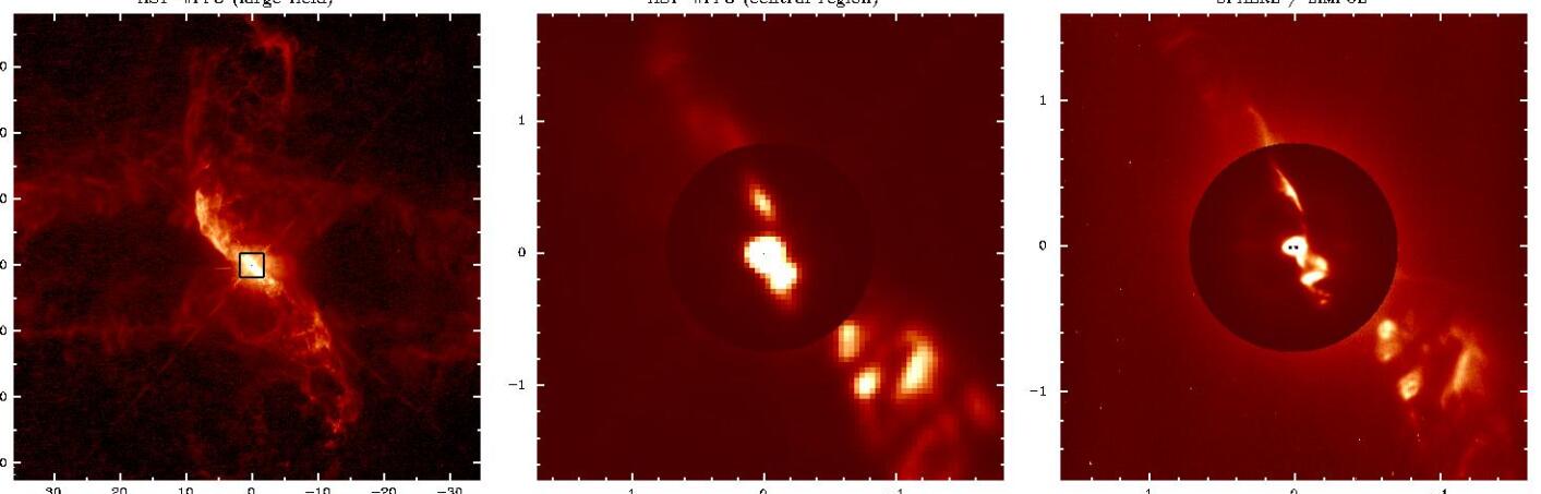
Figure 1: H$\alpha$ images of R Aqr from HST-WFC3 and VLT-SPHERE-ZIMPOL taken in October 2014. The left panel shows a $70^{\prime\prime}\times 70^{\prime\prime}$ cutout of the WFC3 image of the strongly structured extended nebula. The middle panel is the $3.5^{\prime\prime}\times 3.5^{\prime\prime}$ region of the WFC3 image of the central star indicated with the square in the left panel. The right panel is the central $3.2^{\prime\prime}\times 3.2^{\prime\prime}$ area imaged with higher spatial resolution using SPHERE-ZIMPOL where also the two stars are marked with black dots. The color scale is 10 times enhanced for the central $r<0.7^{\prime\prime}$ region in the middle and the right panel. North is up and East to the left.

1 Introduction

R Aqr is a peculiar mira variable with a pulsation period of 387 days surrounded by an extended emission line nebulosity (e.g., Lampland 1922; Hollis et al. 1999). Detailed studies in many wavelength bands revealed that R Aqr is a symbiotic binary with a mass-losing, pulsating red giant and an accreting hot companion with a jet outflow which ionizes an emission nebula. R Aqr is thus an interesting system, and because of its proximity to the sun it became a prototype object for studies on stellar jet, symbiotic (nova-like) activity, mass transfer, and mass loss in interacting binaries.

The orbital period of the R Aqr binary is about $P\approx 44$ years as inferred from periodic phases of reduced brightness observed around 1890, 1933, and 1977 (Willson et al. 1981). These phases are interpreted as partial obscurations of the mira by the companion with its accretion disk and the associated gas and dust flows. The inferred orbital period is supported by radial velocity measurements (see Hinkle et al. 1989; Gromadzki & Mikołajewska 2009).

The R Aqr system was extensively studied with many kinds of high resolution imaging techniques since the first reports about the appearance of a “brilliant emission jet or spike” in 1980 (Wallerstein & Greenstein 1980; Herbig 1980). The structure and motion of jet outflow features was observed with long slit spectroscopy (Solf & Ulrich 1985), radio interferometry (e.g., Hollis et al. 1985; Kafatos et al. 1989; Dougherty et al. 1995), imaging with the Hubble Space Telescope (HST) (Paresce & Hack 1994; Hollis et al. 1997a), and Chandra X-ray observations (Kellogg et al. 2001), while the photosphere of the mira variable and its immediate surroundings were investigated with maser line radio interferometry (e.g., Hollis et al. 2001; Cotton et al. 2004; Ragland et al. 2008; Kamohara et al. 2010), and infrared (IR) interferometry (Ragland et al. 2008; Zhao-Geisler et al. 2012).

We present new high resolution observations of the central jet outflow of R Aqr taken with the new SPHERE (the Spectro-Polarimetric High-contrast Exoplanet REsearch) “Planet Finder” instrument at the Very Large Telescope (VLT) (Beuzit et al. 2008). The Zurich IMaging POLarimeter (ZIMPOL), the visible camera subsystem of SPHERE, provides imaging (and polarimetric imaging) with a resolution of about 25 mas for nebular lines, in particular the prominent H$\alpha$ emission. R Aqr was observed during the instrument commissioning, because this bright star with circumstellar emission is ideal for on-sky tests of line filter observations and imaging polarimetry. Fortunately, one of our test runs took place just a few days before HST - WFC3 line filter observation or R Aqr. This provides a unique opportunity for improving the ZIMPOL flux measurements and the instrument throughput calibration.

For the scientific investigation of the R Aqr system the HST and SPHERE data are very complementary. HST provides a much larger field of view, higher sensitivity, and flux fidelity, while ZIMPOL-SPHERE yields imaging and polarimetric imaging with about three times higher spatial resolution and higher contrast in a small field ($3.6^{\prime\prime}\times 3.6^{\prime\prime}$) centered on the star. The enhanced resolution enables ZIMPOL-SPHERE to resolve the central binary system, the innermost jet clouds, and polarized light produced by the scattering from circumstellar dust particles.

In this work we concentrate the scientific investigation on the SPHERE and HST line filter observations for the small central field of R Aqr. Key topics are the imaging of the central binary and the properties of the innermost jet clouds. We put particular emphasis on accurate absolute flux measurements for the central jet source and the H$\alpha$ cloud components seen in the ZIMPOL data. This is a notoriously difficult task for observations taken with ground based adaptive optics (AO) systems and therefore we want to take advantage of the quasi-simultaneous HST data. The SPHERE-ZIMPOL imaging polarimetry of R Aqr will be presented in a future paper.

Figure 1 gives a first overview of the new H$\alpha$-maps. The HST images from October 2014 show the central part of the extended nebulosity consisting of an inclined ring with a semi-major axis of about 42 arcsec oriented in an E-W direction with an inclination angle of about 70 degrees. In Fig. 1 (left) only the near and far side of the apparent ellipse are visible, about 10^′′ above and below the star. There is also the elongated two-sided jet structure in NE and SW directions and associated arcs extending to about 30 arcsec from the central source. The bright “jet spike” initially detected around 1980 has moved radially out with an angular speed of about $0.2^{\prime\prime}$/yr (e.g., Mäkinen et al. 2004a) and it is now the prominent elongated feature at about 10 arcsec to the NE of the central source.

The jet outflow pattern in R Aqr is quite complex with measured proper motions corresponding to tangential speeds between 50 and 250 kms/s and radial velocities from $-100$ km/s to $+100$ km/s (Solf & Ulrich 1985; Hollis et al. 1997a; Navarro et al. 2003; Mäkinen et al. 2004a). The overall flow pattern of the NE jet spike corresponds to an outflow away from the central binary, with a velocity of about 150 km/s and a radial velocity component of $-70$ km/s (towards us). The SW jet moves roughly in the opposite direction.

Modeling (e.g., Burgarella et al. 1992; Contini & Formiggini 2003) of mainly the bright NE-jet feature, but also other clouds at separations of $>1$ arcsec, indicates that the ionized gas is produced by shocks caused by the interaction of a fast ($v>100$ km/s), collimated outflow from the central binary with slower material ($v<40$ km/s) in the system.

The H$\alpha$ image for the very bright central region with the stellar R Aqr source is shown in Fig. 1b for HST-WFC3 and in Fig. 1c for SPHERE-ZIMPOL. Because of the higher resolution of ZIMPOL, it is possible to resolve the central binary (marked with two dots) and the innermost jet clouds, and we can measure for the first time the exact separation and orientation of the stars.

Jet outflow components at separations of $<0.5^{\prime\prime}$ from the mira have been detected previously with HST imaging and radio interferometry (Paresce & Hack 1994; Dougherty et al. 1995). These studies show a strong variability of the innermost jet structures. Possibly, the binary was already previously resolved by Hollis et al. (1997b) with a map of quasi-simultaneous observation of SiO maser emission from the red giant located about 50 mas south of an extended radio continuum emission, which was associated with the jet source. Unfortunately no second epoch data were published which confirm this. It was also possible to observe the mira photosphere and circumstellar maser emission with a resolution in the 1-10 milli-arcsec range (e.g., Ragland et al. 2008), but the relative location of the companion star could not be constrained from such observations. The new data presented in this work provide images of the central jet outflow with much improved resolution and sensitivity, and they resolve clearly the two stellar components in the system.

This paper is organized as follows. Section 2 gives an overview on the VLT-SPHERE observations, a description of the used filters, and an assessment of the SPHERE AO performance for the R Aqr observations. In Section 3 we determine the relative astrometric position for the central binary. Section 4 provides the photometry for the mira variable in R Aqr and the flux for the total H$\alpha$ emission in the ZIMPOL field. The structures of the observed jet clouds are described in Section 5 including cloud position and size, and the derivation of the H$\alpha$ surface brightness and flux for the individual clouds. Section 6 describes the used HST line filter data and the determination of HST line fluxes. Physical parameters for the jet clouds are derived and analyzed in Section 7 and the final Section 8 puts our new detections on the binary geometry and the jet structure into context with previous and future R Aqr observations.

2 SPHERE / ZIMPOL observations

2.1 The SPHERE / ZIMPOL instrument

The SPHERE “Planet Finder” instrument was successfully installed and commissioned in 2014 at the VLT. SPHERE is optimized for high contrast and high spatial resolution observation in the near-IR and the visual spectral region using an extreme AO system, stellar coronagraphs, and three focal plane instruments for differential imaging. Technical descriptions of the instrument are given in, for example, Beuzit et al. (2008), Kasper et al. (2012), Dohlen et al. (2006), Fusco et al. (2014), and references therein, and much basic information can be found in the SPHERE user manual and related technical websites of the European Southern Observatory (ESO). A first series of SPHERE science papers demonstrate the performance of various observing modes of this instrument (e.g., Vigan et al. 2016; Maire et al. 2016; Zurlo et al. 2016; Bonnefoy et al. 2016; Boccaletti et al. 2015; Thalmann et al. 2015; Kervella et al. 2016; Garufi et al. 2016).

ZIMPOL is one of three focal plane subsystems within SPHERE working in the spectral range from 520 nm to 900 nm (Schmid et al. 2006; Thalmann et al. 2008; Roelfsema et al. 2010; Bazzon et al. 2012; Schmid et al. 2012). ZIMPOL provides differential imaging modes including angular differential imaging (ADI), spectral differential imaging (SDI), and polarimetric differential imaging (PDI). It is designed to take advantage of the high spatial resolution ($\approx$ 20-30 mas) offered by the VLT and the SPHERE extreme AO system, and the high contrast capabilities of the SPHERE visible coronagraph.

ZIMPOL has two camera arms, camera 1 and camera 2, and data are always taken simultaneously in both arms, each equipped with its own filter wheel (FW1 and FW2). This allows us to take data in two different filters simultaneously for SDI. One can also use two equal filters in the two arms or use for both detectors the same filter located in wheel FW0 in the preceding common path.

The pixel scale of ZIMPOL is $3.601\pm 0.005$ mas/pix (mas: milli-arcsec) according to a preliminary astrometric calibration (Ginski et al., in preparation). The position angle of the vertical frame axis is $-2.0\pm 0.5$ degrees with respect to north for both cameras. This offset angle applies for preprocessed data which have been flipped up-down and for camera 2 also left-right to put N up and E to the left. The field of view of the 1k x 1k detectors is $3.6^{\prime\prime}\times 3.6^{\prime\prime}$. Observations are only possible within $4^{\prime\prime}$ from a star with an averaged magnitude $m\;\hbox to0.0pt{\lower 2.5pt\hbox{$\sim$}\hss}\raise 1.5pt\hbox{$<$}\;10^{m}$ for the range 500 – 900 nm, which is bright enough to be used as AO wave front source.

Photometric calibration standard stars are observed regularly for the throughput calibration of the instrument. In this work we report photometric zero points for some filters based on preliminary instrument throughput measurements (Schmid et al., in preparation). Similar high resolution imaging capabilities in the visual range are currently also offered by the VisAO science camera of the MagAO system (without polarimetry) at the 6.5m Magellan telescope (Close et al. 2014) and the VAMPIRES aperture masking interferometer using the SCExAO system at the Subaru telescope (Norris et al. 2015).

Table 1: R Aqr observational data from the SPHERE commissioning.

frame	inst/det	filters			DIT	nDIT	nEXP	dc	remark
identifications	mode	FW0	FW1	FW2	[s]
2014-08-12
OBS224_0092	imaging	–	B_Ha	Cnt_Ha	100	3	1	0.4	peak (RG) saturated
OBS224_0093	imaging	–	Cnt_Ha	B_Ha	100	3	1	0.4	peak (RG) saturated
OBS224_0094	imaging	–	Cnt_Ha	N_Ha	100	3	1	0.4	Cnt_Ha (RG) saturated
OBS224_0095	imaging	V_S	–	–	20	3	1	0.1
OBS224_0096	imaging	OI_630	–	–	100	3	1	0.4
OBS224_0097	imaging	HeI	–	–	100	3	1	0.4
2014-10-11
OBS284_0030–34	imaging	N_Ha	–	–	40	1	5	0.2	with dithering
OBS284_0035–38	imaging	N_Ha	–	–	200	1	4	0.8	off-axis fields
OBS284_0051–54	slow pol.	–	CntHa	N_Ha	50	2	4	4.0
OBS284_0039–42	fast pol.	–	V	V	1.2	10	4	$<0.1$
OBS284_0055–58	slow pol.	–	V	V	10	4	4	$<0.1$
OBS284_0043–46	fast pol.	–	TiO_717	Cnt748	1.2	10	4	$<0.1$
OBS284_0047–50	fast pol.	–	Cnt820	Cnt820	1.2	10	4	$<0.1$
OBS284_0059–62	fast pol.	–	I_PRIM	I_PRIM	1.2	10	4	$<0.1$	peak saturated
OBS284_0063–70	fast pol.	–	I_PRIM	I_PRIM	5	6	8	$<0.1$	coronagraphic
OBS284_0071–74	slow pol.	–	I_PRIM	I_PRIM	10	20	4	$0.8$	coronagraphic

2.2 SPHERE / ZIMPOL data

R Aqr was used as a test source for the verification of different instrument configurations and therefore the observations are not optimized for scientific purposes. The data are affected by several technical problems, especially for the July run when no scientifically useful data could be obtained. In August 2014 only imaging observations were possible, but no imaging polarimetry. The data from October 2014 could be taken without technical problems. For the scientific investigation of R Aqr we use only the data from August and October 2014 listed in Table 1. All data were taken in field-stabilized mode without field position angle offset and using the gray beam splitter sending about 21 % of the light to the wave front sensor (WFS) and transmitting 79 % to the ZIMPOL instrument.

The R Aqr mira variable has a pulsation period of 387.3 days (Gromadzki & Mikołajewska 2009). In October 2014 the mira brightness was, according to the light curve of the American Association of Variable Star Observers (AAVSO), at its minimum phase with $m_{\rm vis}\approx 11$ mag. This is ideal for the imaging of the R Aqr jet. In mid August 2014 the visual magnitude was about 1 mag brighter. At maximum the system reaches a visual brightness of $m_{\rm vis}\approx 6$ mag.

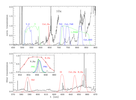
Figure 2: R Aqr spectrum from 2010/2011 and transmission curves of the used ZIMPOL continuum filters (upper panel) and line filters (lower panel). The flux scale for the R Aqr spectrum is arbitrary, but the short wavelength part $\lambda<700$ nm in the upper panel is multiplied by a factor of ten for better visibility.

The selected filters cover a wide wavelength range using the broad band V-filter where R Aqr is faint, and narrow band filters at longer wavelength where the system is bright. The filter passbands are shown in Fig. 2 together with R Aqr spectra taken by Christian Buil in August 2010 (spectrum $\lambda=670-900$ nm) and September 2011 ($\lambda<700$ nm and emission line spectrum) during similar brightness phases of R Aqr as our SPHERE data. These spectra are available in the database of ARAS (Astronomical Ring for Access to Spectroscopy). We took also broad-band I_PRIM data for an investigation of the dynamic range of the polarimetric mode which will be discussed in a future paper. These data are either saturated or taken with a coronagraph and therefore not useful for photometry.

The emission nebula of R Aqr was observed with all ZIMPOL line filters, in particular the different types and combination possibilities of the H$\alpha$ filters. The narrow N_Ha filters with a width of $\approx 1$ nm are optimized for continuum rejection with the disadvantage that the transmission changes rapidly for emission which is slightly shifted in wavelength. It should be noted that the N_Ha filter in the common filter wheel FW0 has its peak at the rest wavelength 656.3 nm of the H$\alpha$ line, while the N_Ha filter in filter wheel FW2 is at 656.5 nm.

In August 2014 all Cnt_Ha and B_Ha filter frames were saturated in the peak of the red giant. In October 2014 one set of N_Ha frames is taken with a five-point dithering pattern. Also four frames covering off-axis fields centered about 2 arcsec to the NE, SE, SW, and NW of R Aqr were taken.

Observations in polarimetric mode were taken in October 2014. We use in this work only the total intensity images of the polarimetric data. The throughput is about 18 % lower because of the inserted polarimetric components. Also the detector mode is changed for on-chip demodulation of the data (see Schmid et al. 2012). In particular, the slow modulation modes has a low detector gain of 1.5 e^-/ct (ct = ADU, analog to digital count units), much lower than the 10.5 e^-/ct gain for imaging and fast polarimetry. The read-out noise of the CCD (charge-coupled device) is about 1-2 ct and this translates for the slow polarimetry into a much lower noise level in terms of photo-electrons e^-, and therefore a better faint source sensitivity, when compared to imaging and fast polarimetry.

2.3 ZIMPOL data reduction

The data reduction of ZIMPOL imaging data is for most steps straight forward and follows standard procedures like bias frame subtraction, cosmic ray removal with a median filter, and flat fielding. The data reduction was performed with the (SPHERE-ZIMPOL) SZ-software package, which is written in IDL and was developed at the ETH (Eidgenössische Technische Hochschule) Zurich. The basic procedures are essentially identical to the SPHERE DRH-software provided by ESO.

A special characteristic of the ZIMPOL detectors are the row masks which cover every second row of the detector. This feature is implemented in ZIMPOL for high precision imaging polarimetry using a modulation-demodulation technique (Schmid et al. 2012). A raw frame taken in imaging mode has only every second row illuminated and the useful science data has a format of $512\times 1024$ pixels consisting of the 512 illuminated rows of the $1024\times 1024$ pixel detector. One pixel represents $7.2\times 3.6$ mas on the sky because of the cylindrical micro lens arrays on the ZIMPOL detectors, and the total image covers about $3.6^{\prime\prime}\times 3.6^{\prime\prime}$ (see Schmid et al. 2012).

The same image format results from polarimetric imaging. In polarimetry, the photoelectric charges are shifted up and down by one row during the integration, synchronously with the polarimetric modulation. In this way the whole detector array is filled with photo electrons with perpendicular and parallel polarization signals stored in the “even” and “odd” rows, respectively. However, the image sampling is identical to the imaging mode with photons only detected at the position of the open detector rows. In this work, only the intensity signal from the polarimetric observations is considered and the “even” and “odd” row counts are added to yield total intensity images with $512\times 1024$ pixels.

In one of the final steps in the data processing, the $512\times 1024$ pixel images are expanded with a flux-conserving linear interpolation to yield a square $1024\times 1024$ pixel image where one pixel represents $3.6\times 3.6$ mas on sky. The artificial oversampling of the image rows has no significant apparent effect on the resulting images.

The detector dark current was found to be variable for our test observations. Therefore, it was not possible to subtract the dark current based on calibration measurements. As an alternative, we determined the dark current from the science frames. In imaging mode one can use, for dark current estimates, the count level in the covered row pixels for detector regions with low illumination, and for polarimetric observations we used the count level in the detector edges (far from the central source) for weakly illuminated frames.

The estimated dark current levels are given in Table 1. Typically the values are small except for longer integrations with the low gain slow polarimetry mode. Nonetheless, a subtraction of a low dark current level of $<1$ ct/pix is still important for flux measurements in large apertures, for example, $r_{\rm ap}>0.1^{\prime\prime}$ with $\gg 10^{3}$ pixels, as described in this study for certain cases.

Table 2: PSF parameters for the red giant in R Aqr and the standard star HD 183143 in different filters.

filter	$\lambda_{c}$	files / cam	$\tau_{0}$	Strehl $S_{0}$	${\rm ct}(r)/{\rm ct}_{\rm 3dia}$ [%]							ct${}_{\rm 1M}/{\rm ct}_{\rm 3dia}$
	[nm]		[ms]	ratio	$r$ [pix] =	0	5	10	30	100	300	[%]
				[%]	npix =	1	81	317	2821	31417	282697
R Aqr, OBS284_xx
V	554	0055-58 / 1+2	3.3	1.9		0.091	5.0	10.5	18.8	42.7	86.9	114
CntHa	645	0051-54 /   1	2.9	4.2		0.151	8.6	18.2	28.7	45.3	86.1	118
max		0051 /   1		5.9		0.215	10.5	19.3	28.7	45.8	86.8
min		0053 /   1		3.2		0.114	7.0	16.0	26.7	43.2	85.2
TiO	717	0043-46 /   1	2.8	8.3		0.244	12.5	23.4	35.1	50.2	89.9	102
Cnt748	747	0043-46 /   2	2.8	10.3		0.280	14.1	25.7	38.3	52.6	91.0	106
Cnt820	817	0047-50 / 1+2	2.7	23.9		0.541	25.4	41.0	54.9	65.3	93.9	103
HD 183143, STD261_xx
V	554	0017-20 / 1+2	8.8	8.8		0.431	18.9	31.9	43.6	65.9	93.6	106
N_R	646	0013-16 / 1+2	8.1	13.5		0.489	21.1	35.9	48.9	66.9	94.4	105
N_I	790	0021-24 / 1+2	8.1	20.9		0.505	24.4	39.9	54.9	69.2	94.7	105

2.4 SPHERE adaptive optics performance for the R Aqr observations

Knowledge of the AO performance and the point spread function (PSF) is important for quantitative photometric measurements from imaging data. No systematic study on the AO performance of SPHERE-ZIMPOL exists up to now. Therefore, we compare the PSFs for R Aqr observations with the PSFs of HD 183143 from the ESO archive (frame: STD261_0013-24 from 2015) which were taken under very good atmospheric conditions. HD 183143 ($m_{V}=6.9^{m}$) is a high polarization standard star which was observed for polarimetric calibrations and as a PSF test source. The azimuthally averaged and normalized PSFs of R Aqr and HD 183143 are plotted in Fig. 3 and approximate Strehl ratios and counts within circular apertures are given in Table 2.

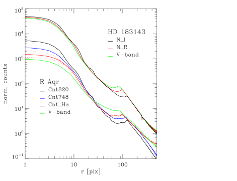
Figure 3: PSFs in different filters for the red giant in R Aqr and the star HD 183143. The PSFs are normalized for R Aqr to a total count level of $10^{6}$ within an aperture of 3 arcsec diameter (lower curves) and for HD 183143 to $10^{7}$ (upper curves). PSF for different filters are given by different colors as indicated. The dashed red curves for R Aqr show the “best” (max) and “worst” (min) PSF for the CntHa-filter observations.

For HD 183143 the radial profiles are given for the V-, N_R-, and N_I-band filters and the total counts are normalized to $10^{7}/{\rm ct}_{\rm 3dia}$, where ${\rm ct}_{\rm 3dia}$ are the counts within an aperture with a diameter of 3 arcsec. The PSFs show clearly the wavelength dependent location of the AO control radius at $\lambda/D=20$ (at $r\approx 100$ pix in Fig. 3) up to which the AO corrects for the wave-front aberrations. Beside this feature the PSFs for the different filters are quite similar with only a very small wavelength dependence in the relative peak counts ${\rm ct(0)}/{\rm ct}_{\rm 3dia}$.

Approximate Strehl ratios $S_{0}$ are derived from the ratio between the measured relative peak counts ${\rm ct(0)}/{\rm ct}_{\rm 3dia}$ and the expected relative peak flux for diffraction-limited PSFs according to

$$S_{0}={{\rm ct(0)/ct}_{\rm 3dia}\over f(0)/f_{\rm 3dia}}\,,$$

where $f(0)/f_{\rm 3dia}$ is calculated for the VLT (8.0 m primary mirror telescope with a 1.1 m central obscuration by the secondary mirror). For a pixel size of $3.6\times 3.6$ mas there is $f(0)/f_{\rm 3dia}=4.95\leavevmode\nobreak\ \%$, 3.66 %, and 2.44 % for the V-, N_R-, and N_I-filters, respectively. Ratios $S_{0}$ between about 9 % and 21 % are obtained for the HD 183143 observations which were taken under good conditions with a long atmospheric coherence time of $\tau_{0}\approx 8-9$ ms.

This kind of approximate Strehl ratio $S_{0}$ determination provides a very useful parameter for a simple comparison of the atmospheric conditions and the AO performance of different data sets taken with ZIMPOL. However, the $S_{0}$ value does not describe well the SPHERE AO system, because of instrumental effects not related to the adaptive optics. A more sophisticated AO characterization should be based on the analysis of the Fourier transform of the aberrated image as described in Sauvage et al. (2007). Such an analysis yields for the N_I-filter PSF of HD 183143 an AO Strehl ratio of 33 % instead of the 22 % indicated in Table 2. The difference can be explained by a residual background at low spatial frequencies of undefined nature, perhaps due to instrumental stray light, not fully corrected detector noise, or other effects.

For R Aqr the PSFs for the V-band, CntHa, Cnt748, and Cnt820 filters are plotted in Fig. 3 and corresponding $S_{0}$-values and relative encircled fluxes are listed in Table 2. These profiles were normalized to the total aperture count of ${\rm ct}_{\rm 3dia}=10^{6}$ to displace them in Fig. 3 from the curves of HD 183143.

The PSFs for R Aqr show a very strong and systematic wavelength dependence in the normalized peak counts ${\rm ct(0)/ct}_{\rm 3dia}$ (Table 2, Fig. 3). For the Cnt820-filter, this value is comparable to the case of HD 183143, but for the V-band filter it is about a factor of five lower than for the Cnt820-filter in R Aqr or the V-band data of HD 183143. There are several reasons for the lower PSF peak in R Aqr at shorter wavelengths: (i) the AO performance was less good than for HD 183143 because the coherence time was shorter $\tau_{0}\approx 3$ ms and this affects mainly the short wavelengths, (ii) the extreme red color of R Aqr could be responsible, because the SPHERE wave-front sensor “sees” essential only I-band light and the AO system cannot correct for additional (differential) aberrations in the V-band, and (iii) the intrinsic PSF of R Aqr is more extended at short wavelength due to scattering of the light by circumstellar dust, some light contributions from the hot binary companion, and/or some extended nebular emission.

The PSFs of R Aqr show also temporal variability which are particularly strong at short wavelengths. Such variations can certainly be associated with strong variability in the atmospheric conditions and the resulting AO performance. We have picked the case of the four CntHa-filter exposures from October 11 for which Fig. 3 and Table 2 give also the parameters for the maximum (“best”) and the minimum (“worst”) PSF. For example, the $S_{0}$ Strehl ratio changes within a few minutes by a factor of almost two.

Because of this strong variability it is difficult to derive accurate photon fluxes for clouds in dense fields which need to be measured with small apertures. It is also difficult to quantify the flux of the extended PSF halo, which should be disentangled from possible diffuse intrinsic emission in the R Aqr system. This problem is taken into account in Sect. 5.3 for the H$\alpha$ flux measurements of the jet clouds.

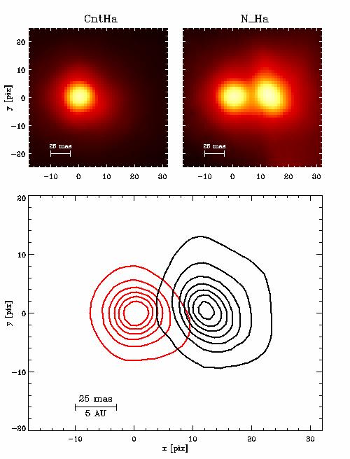
Figure 4: R Aqr central binary as seen in the CntHa (top left) and the N_Ha (top right) filters on October 11, 2014 (OBS284_0051). The contour plot shows the red giant for the CntHa filter (red) and the ”pure” H$\alpha$ emission in the N_Ha image after subtraction of the scaled and aligned CntHa frame (black). Contour levels are given for seven levels from 1000 to 7000 ct/pix.

3 Astrometry of the central binary star system

The R Aqr images taken with SPHERE-ZIMPOL show in all filters, except the H$\alpha$ filters, one strongly dominating point source from the mira variable. Contrary to this, all H$\alpha$ images show in the center two point-like sources (Fig. 4) and additional weaker emission features in an NE and SW direction. The central H$\alpha$ source has a peak flux which is more than ten times stronger than all other H$\alpha$ features. The central H$\alpha$ source is located about 12 – 13 pixel ($\approx 45$ mas) to the W of the mira variable which is the expected binary separation for the R Aqr system (e.g., Gromadzki & Mikołajewska 2009). The central H$\alpha$ is slightly extended in the NE–SW jet direction (Fig. 4b and c). Figure 5 shows E-W profiles through the two source peaks for the different H$\alpha$ filter observations.

The bright point-like H$\alpha$ source, just besides the mira in R Aqr, is very likely the compact emission region around the active companion, which is at the same time the jet source of the system. Thus, our high resolution H$\alpha$ images provide the unique opportunity for an accurate measurement of the binary separation and orientation for the R Aqr system, and with future observations it should be possible to determine accurate orbital parameters and stellar masses.

Ideal for accurate astrometric measurements are the N_Ha data from October 11, 2014 in which the two stellar sources have about the same brightness. For this date the mira was at its minimum phase, and about a factor 2.4 fainter (peak intensity) than in the N_Ha data of August 12. In the B_Ha images of the same date, the mira variable is much brighter and saturated because of the wider band pass (see Fig. 5).

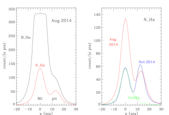
Figure 5: East-west cuts through the R Aqr binary system for different H$\alpha$ filter observations taken in imaging mode. Left: B_Ha and N_Ha profiles from August 12, 2014, showing the much reduced continuum throughput in N_Ha (the peak of B_Ha is strongly saturated); Right: N_Ha profiles for August 12, 2014 and October 11, 2014 illustrating the brightness change of the red giant within 60 days. The dotted green curve shows the scaled red giant profile as seen in the CntHa filter (slow pol. mode) from October 11.

The simultaneous observations in the Cnt_Ha in camera 1 and the N_Ha in camera 2 from October 11 (OBS28_0051-54) provide as an additional advantage a binary image and a “reference PSF” for the mira with the same PSF distortions. From this set we selected the “best” or maximum PSF exposure (OBS284_0051, Table 2). We centered the CntHa PSF of the red giant and used it as astrometric zero point (Fig. 4a). Then we subtracted a scaled version of this frame from the N_Ha double star image (Fig. 4b), which was shifted around in steps of 0.1 pixels in $\Delta x$ and $\Delta y$ until the subtraction yields “a clean H$\alpha$” source image (Fig. 4c) with a minimal residual pattern at the zero point, that is, at the location of the subtracted red giant PSF. A centroid fit to the H$\alpha$ source center yields then the following relative position of the H$\alpha$ source with respect to the red giant:

$$\Delta x=12.54\pm 0.10\leavevmode\nobreak\ {\rm pix}\,, \Delta y=0.54\pm 0.10\leavevmode\nobreak\ {\rm pix}\,,$$ (1)

$$\Delta\alpha=-45.1\pm 0.6\leavevmode\nobreak\ {\rm mas}\,, \Delta\delta=0.4\pm 0.6\leavevmode\nobreak\ {\rm mas}\,.$$ (2)

This corresponds with the astrometric calibration given in Sect. 2.1 to a position angle of $270.5^{\circ}\pm 0.8$ (measured N over E) and a separation of $45.1\pm 0.6$ mas. This translates for an R Aqr distance of 218 pc (Min et al. 2014) into an apparent separation of 9.8 AU.

It is unclear how well this astrometric result for the photo-centers represents the positions of the mass centers of the two stellar components. The mira variable shows a photosphere with an asymmetric light distribution (Ragland et al. 2008) and for the jet source it seems likely that the measured H$\alpha$ emission peak is not exactly at the position of the invisible stellar source probably located in an accretion disk.

Therefore, the position of the photo-center could deviate from the mass center of the stellar components by more than the indicated photo-center measurement uncertainties of $\approx 0.5$ mas. Future observations will show how well one can determine the orbit from the photo-center measurements. In any case we can expect a significant reduction of uncertainties for the orbital parameters of R Aqr.

Table 3: R Aqr red giant continuum photometry for an aperture of $3.6^{\prime\prime}\times 3.6^{\prime\prime}$.

filter	files / cam	mode	ct1M	ct/s	${\rm am}\cdot k_{1}$	$m_{\rm mode}$	$zp_{\rm ima}$	$m(F)$
			[$10^{6}$]	[$10^{6}$/s]	[mag]	[mag]	[mag]	[mag]
date: 2014-08-12, OBS224_xx
V_S	0095 / 1+2	imaging	$1.38\pm 0.06$	0.0688	0.19	0.0	22.72	$10.4\pm 0.1$
HeI	0097 / 1+2	imaging	$5.27\pm 0.15$	0.0527	0.18	0.0	20.77	$8.8\pm 0.1$
OI	0096 / 1+2	imaging	$5.32\pm 0.15$	0.0531	0.15	0.0	20.67	$8.7\pm 0.1$
date: 2014-10-11, OBS284_xx
V	0055-58 / 1+2	slow pol.	$5.55\pm 0.24$	0.551	0.15	-1.93	23.70	$11.3\pm 0.1$
V	0039-42 / 1+2	fast pol.	$0.073\pm 0.034$	0.058	0.15	0.18	23.70	$11.5\pm 0.3$
Cnt_Ha	0051-54 /   1	slow pol.	$13.1\pm 0.6$	0.262	0.10	-1.93	20.35	$8.8\pm 0.1$
TiO_717	0043-46 /   1	fast pol.	$0.307\pm 0.021$	0.244	0.09	0.18	21.78	$8.0\pm 0.1$
Cnt748	0043-46 /   2	fast pol.	$1.05\pm 0.03$	0.836	0.08	0.18	21.68	$6.6\pm 0.1$
Cnt820	0047-50 / 1+2	fast pol.	$4.16\pm 0.09$	3.31	0.08	0.18	20.97	$4.4\pm 0.1$

4 ZIMPOL aperture photometry

4.1 Aperture photometry for the red giant

R Aqr shows strong, periodic brightness variations between $m_{\rm vis}\approx 6.5^{m}$ and 11.0^m. We derive photometric magnitudes of the mira variable for our ZIMPOL filter observation which are useful for the absolute H$\alpha$ line fluxes of the jet clouds, the determination of upper flux limits for the hot companion, and for estimates of the flux contribution of the mira star to the HST line filter images. Photometric magnitudes are obtained by summing up all counts “ct_1M” registered in the $10^{6}$ pixels area [$x_{1}$:$x_{2}$,$y_{1}$:$y_{2}$] = [13:1012,13:1012] of the $1024\times 1024$ pixel detector. This is equivalent to photometry with an aperture of $3.6^{\prime\prime}\times 3.6^{\prime\prime}$ using essentially the whole detector except for the outermost rows and columns of the CCD, which are partly hidden by the frame holding the microlens array of the detector (see Schmid et al. 2012).

The obtained counts ${\rm ct}_{\rm 1M}$ per frame and detector arm are listed in column 4 of Table 3. The indicated measuring uncertainty is composed of three error sources; a relative factor of $\pm 0.02\cdot{\rm ct}_{\rm 1M}$ which accounts for sky transparency and instrument throughput variations, a bias subtraction uncertainty of $\pm 20000$ ct equivalent of 0.02 counts/pixel, and a relative uncertainty in the dark current subtraction of $\pm 20\leavevmode\nobreak\$% which becomes more important than the bias subtraction uncertainty for a dark current $>0.1$ ct/pix. These contributions are treated like independent errors and are combined by the square-root of the sum of the squares.

Count rates ct/s (Table 3) are obtained by dividing ${\rm ct}_{\rm 1M}$ with the detector integration time (DIT). A small correction for the frame transfer time (ftt) is required ${\rm ct/s}={\rm ct}_{\rm 1M}/({\rm DIT}+{\rm ftt})$ because the detector is also illuminated during the short frame transfer, which is ${\rm fft}=56$ ms for imaging and fast polarimetry and ${\rm fft}=74$ ms for slow polarimetry (Schmid et al. 2012). The frame transfer time correction is only relevant ($>1\leavevmode\nobreak\ \%$) for short DIT $<7$ s.

In the next step the count rates in a given filter $F$ are converted to photometric magnitudes $m(F)$ using the formula

$$m(F)=-2.5\,{\rm log}\,({\rm cts/s})-{\rm am}\cdot k_{1}(F)-m_{\rm mode}+zp_{\rm ima}(F)\,.$$ (3)

This accounts for the atmospheric extinction with a filter and airmass dependent correction ${\rm am}\cdot k_{1}(F)$ (Table 3) using the Paranal extinction curve from Patat et al. (2011). The airmass for our R Aqr observations was in the range ${\rm am}=1.31-1.46$ for Aug. 12 and ${\rm am}=1.11-1.15$ for Oct. 11.

The photometric zero points $zp_{\rm ima}(F)$ for the individual filters were determined with calibration measurements of the spectrophotometric standard star HR 9087 (Hamuy et al. 1992), which will be described in Schmid et al. (2016, in prep.). The $zp_{\rm ima}(F)$-values apply for the ZIMPOL imaging mode with the gray beam-splitter between wave front sensor and ZIMPOL. For other instrument modes one needs in addition a throughput offset parameter $m_{\rm mode}$. For example, for polarimetry, $m_{\rm mode}=0.18$ accounts for the reduced transmission because of the inserted polarimetric components. The difference of $\Delta m_{\rm mode}=-2.11$ between fast and slow polarimetry is because of the changed detector gain factor from 10.5 e^-/ct in fast polarimetry to 1.5 e^-/ct in slow polarimetry.

The zero point values $zp_{\rm ima}(F)$ given in Table 3 are preliminary and the estimated uncertainties are about $\pm 0.10$ mag and this dominates the error in the final magnitudes except for the underexposed V-band (fast polarimetry) observations. For such low illumination, the uncertainty of ($\pm 0.02$ ct/pix) in the bias level is an issue in the “full detector” aperture photometry.

R Aqr was observed with different filters in August and October 2014. We may compare the V_S ($\lambda_{c}=532$ nm) magnitude $m_{\rm V\_S}=10.4^{m}$ from August 11 with $m_{V}=11.4^{m}$ ($\lambda_{c}=554$ nm). This gives a decrease in brightness of about 1 mag within 60 days in good agreement with the AAVSO light curve (see Sect. 2).

The obtained magnitudes (Table 3) indicate for October 11, 2014 very red colors of V – CntHa = 2.5^m and V – Cnt820 = 6.9^m for R Aqr. Because R Aqr is strongly variable, these colors cannot be compared readily with literature values. Celis S. (1982) measures also a very red color of V – I = 7.8^m in Johnson filters for the R Aqr minimum epoch from Nov. 1981.

Table 4: H$\alpha$ absolute “aperture” photometry for R Aqr.

flux	ct1M/s	flux
component	[kct/s]
date: 2014-08-12, OBS224_0092+93 / 1+2
B_Ha total	$>228$
H$\alpha$ only	$44\pm 20$	$35(\pm 16)\cdot 10^{-12}$
RG only	$>184$	$>2.4\cdot 10^{-12}$
date: 2014-08-12, OBS224_0094 / 2
N_Ha (FW2)	$81\pm 5$
H$\alpha$ only	$48\pm 17$	$64(\pm 23)\cdot 10^{-12}$
RG only	$33\pm 17$	$3.6(\pm 1.8)\cdot 10^{-12}$
date: 2014-10-11, OBS284_0030-34 / 1+2
N_Ha (FW0)	$63\pm 7$
H$\alpha$ only	$42\pm 12$	$38(\pm 10)\cdot 10^{-12}$
RG only	$21\pm 12$	$2.2(\pm 1.1)\cdot 10^{-12}$
date: 2014-10-11, OBS284_0051 / 2
N_Ha (FW2)	$330\pm 16$
H$\alpha$ only	$256\pm 25$	$43(\pm 10)\cdot 10^{-12}$
RG only	$74\pm 25$	$1.4(\pm 0.4)\cdot 10^{-12}$
weighted mean
H$\alpha$ only	$F_{\rm 1M}({\rm H}\alpha)$	$42(\pm 7)\cdot 10^{-12}$

4.2 Total H$\alpha$ flux within $3.6^{\prime\prime}\times 3.6^{\prime\prime}$

Absolute photometry is required for the determination of the H$\alpha$ flux of jet clouds for the determination of intrinsic line emissivities $\epsilon({\rm H}\alpha)$. A first complicating factor is that the bright red giant is a strongly variable source and therefore a bad flux reference source. A second complicating factor are the complex structures of the H$\alpha$ emission features, composed of small and large, bright and faint clouds, and perhaps even a diffuse emission component. The flux measurements require therefore the definition of flux apertures and appropriate aperture correction factors, and this introduces additional measuring uncertainties. The quasi simultaneous HST data are very helpful to improve and check the ZIMPOL flux measurements but in the HST data some clouds are blended and aperture correction factors differ because of the lower spatial resolution.

For this reason we determine here also the total H$\alpha$ flux for the central $3.6^{\prime\prime}\times 3.6^{\prime\prime}$ region of R Aqr. This value is independent of the flux aperture definition and correction factors, but needs to account properly for the contribution of the red giant. Therefore, this provides an alternative H$\alpha$ flux comparison with the HST data. The total H$\alpha$ flux in a large aperture allows also a flux comparison with seeing-limited spectrophotometric measurements.

We have taken different H$\alpha$ filter observations of R Aqr, simultaneous CntHa / B_Ha filter data on August 12, simultaneous CntHa / N_Ha(FW2) data on August 12 and October 11 and N_Ha(FW0) data in both channels on August 12. The total frame count rates ct_1M/s are given in Table 4. Two steps are required for the conversion of these measurements into a total H$\alpha$ flux for the innermost $3.6^{\prime\prime}\times 3.6^{\prime\prime}$ R Aqr nebulosity: (i) the emission of the red giant must be subtracted from the extended H$\alpha$ emission, and (ii) the conversion of the count rates into a continuum flux for the red giant and a line flux for H$\alpha$ using photometric zero points.

Table 4 splits the total count rates into count rates for the H$\alpha$ line and red giant continuum. This is achieved with a subtraction of the scaled CntHa image from OBS284_0051 as demonstrated for our astrometry of the central binary in Sect. 3. This H$\alpha$ measuring procedure is accurate ($\approx\pm 10\leavevmode\nobreak\ \%$) for the simultaneous N_Ha frame (OBS284_0051).

For all other H$\alpha$ observations, there exist no simultaneous, unsaturated CntHa frames for the flux splitting. Subtracting non-simultaneous CntHa frames from H$\alpha$ data is less accurate because of the AO performance variations described in Sect. 2.4. Matching the PSF peak of the red giant might not account well for the total red giant flux in the H$\alpha$ image, which is mostly ($>80\leavevmode\nobreak\ \%$) contained in the extended halos at $r>10$ pix. Therefore the flux splitting is less accurate ($\approx\pm 25\leavevmode\nobreak\ \%$) for the OBS284_0030-34 data taken 15 minutes before the red giant PSF, and the uncertainty is substantial ($\approx\pm 35-50\leavevmode\nobreak\ \%$) for the H$\alpha$ flux from August 12 because then the red giant was brighter and even saturated in the B_Ha data.

The conversion of the count rates ${\rm ct}_{\rm 1M}/{\rm s}$ measured in a given H$\alpha$-filter “$F$” into an emission line flux $f({\rm H}\alpha)$ [erg cm^-1s^-1] or into a red giant continuum flux $f(F)$ [erg cm^-1s${}^{-1}{\rm\AA}^{-1}$] follows from the following formula

$$f={\rm ct_{\rm 1M}/s}\cdot 10^{\,0.4\,(am\cdot k_{1}+m_{\rm mode})}\cdot c_{\rm zp}(F)\,,$$ (4)

where $c_{\rm zp}(F)$ is either the photometric zero point for the H$\alpha$ line emission $c_{\rm zp}^{\ell}(F)$ or for the continuum emission $c_{\rm zp}^{\rm cont}(F)$. The zero point values $c_{\rm zp}$ for the different H$\alpha$ filters are given in Table 5. They are based on calibration measurements of the Vega-like spectrophotometric standard star HR 9087 for which the stellar H$\alpha$ absorption has been taken into account. A detailed description of the ZIMPOL filter zero point determination is planned for a future paper. The atmospheric extinction correction is $0.10^{m}\pm 0.01^{m}$ and $m_{\rm mode}$-values are $0^{m}$ for imaging, $+0.18^{m}$ for fast polarimetry, and $-1.93^{m}$ for slow polarimetry as described in Sect. 4.1.

The line flux conversion $c_{\rm zp}^{\ell}$ depends on the wavelength of the line emission within the filter transmission curve. This is a particularly important issue for the very narrow transmission profiles of the N_Ha filters (see Fig. 2). For example, the transmission in the N_Ha filters is reduced by 25 % for an offset of $\Delta\lambda=\pm 0.3\leavevmode\nobreak\ {\rm nm}$ ($\Delta{\rm RV}=\pm 137$ km/s) from $\lambda_{\rm c}$. The enhanced uncertainties for $c_{\rm zp}^{\ell}$ for the N_Ha filters in Table 5 take this problem into account. Of course, high velocity H$\alpha$ gas with $|RV|\gg 100$ km/s is not detected with the N_Ha filters.

We adopt a heliocentric radial velocity (RV) of $-25$ km/s for the H$\alpha$ emission peak of R Aqr, because the measured values lie between $0$ and $-50$ km/s (e.g., Van Winckel et al. 1993; Solf & Ulrich 1985) and they agree well also with the systemic radial velocity of $-24.9$ km/s derived from the radial velocity curve of the mira by Gromadzki & Mikołajewska (2009). This yields for our observing dates a geocentric RV of about $-30$ km/s and $-5$ km/s for the H$\alpha$ line, or shifts of less than 0.1 nm with respect to the H$\alpha$ rest wavelength in air of 656.28 nm. This matches well with the peak transmission wavelengths $\lambda_{c}=656.34$ for the N_Ha filter located in FW0 and therefore the expected transmission is about $T=0.7$. The match with the peak wavelength $\lambda_{c}=656.53$ for the N_Ha located in FW2 is less good and the expected transmission is only about $T=0.5$. These values are used for the H$\alpha$ line flux determinations for the N_Ha filters given in Table 4.

Table 5: ZIMPOL H$\alpha$ filter parameters for the filter B_Ha, N_Ha (FW0 and FW2) and CntHa.

value [unit]	B_Ha	N_Ha	N_Ha	CntHa
		(FW0)	(FW2)
$\lambda_{\rm c}$ [nm]	655.6	656.34	656.53	644.9
FWHM [nm]	5.5	1.15	0.97	4.1
$T_{\rm peak}$	0.89	0.76	0.70	0.87
$\Delta\lambda$ [nm]	5.35	0.81	0.75	3.83
$c^{\ell}_{\rm zp}$	7.2	8.4	9.2	…
	$(\pm 0.4)$	$(^{+2.0}_{-0.5})$	$(^{+4.0}_{-0.5})$
$c^{\rm cont}_{\rm zp}$	1.20	9.3	10.0	1.59
	$(\pm 0.05)$	$(\pm 0.5)$	$(\pm 0.5)$	$(\pm 0.05)$

H$\alpha$ wavelength shifts are much less critical for the broader, 5 nm wide B_Ha filters. But the B_Ha photometry could be contaminated by the nebular [N II] emission located at 654.8 and 658.3 nm (see Fig. 2). For the central region of R Aqr, the H$\alpha$ emission is about ten times stronger than [N II] as follows from the spectrum shown in Fig. 2 or the HST fluxes given in Table 9. Table 4 lists the resulting flux values and we use in the following the weighted mean value $F_{\rm 1M}({\rm H}\alpha)$ for the H$\alpha$ line flux within the $3.6^{\prime\prime}\times 3.6^{\prime\prime}$ central area. Better results could be obtained with simultaneous, non-saturated B_Ha / CntHa measurements, because the broader line filter is less affected by H$\alpha$ radial velocity shifts. An additional measurement in the N_Ha / CntHa filter could be useful, if the disturbing continuum emission is strong, or if contamination by [N II] emission is an issue. Previous spectroscopic observations by Van Winckel et al. (1993) give 26 and $40\cdot 10^{-12}{\rm erg\,s}^{-1}{\rm cm}^{-2}$ for the H$\alpha$ flux of R Aqr for two epochs in 1988. Thus the total H$\alpha$ flux is on a similar level as 25 years ago.

5 ZIMPOL photometry for the jet clouds

5.1 Overview on the H$\alpha$ jet cloud structure

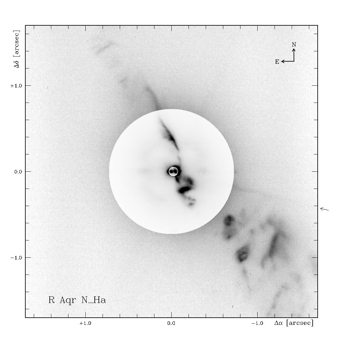
Figure 6: Map of the SPHERE-ZIMPOL H$\alpha$ line observation of R Aqr taken in the N_Ha (FW0) filter on Oct. 11, 2014. The field is divided into three different gray scale regions ranging from 0 to 1000 ct pix^-1frame^-1 for the central binary, 0 to 100 for the inner jet region $r_{\rm RG}<0.72^{\prime\prime}$ , and 0 to 10 for the outer jet region $r_{\rm RG}>0.72^{\prime\prime}$. The red giant is at the zero point of the coordinate system. There is a small angle offset of 2 degr of the sky N orientation in a counter-clockwise direction with respect the (vertical) $y$-direction. A weak instrumental spike from a telescope spider is present at a position angle of about $-105^{\circ}$ indicated by a small arrow outside the frame.

The H$\alpha$ map plotted in Figure 6 shows the very rich nebular emission within the central $3.4^{\prime\prime}\times 3.4^{\prime\prime}$ region of R Aqr based on the five dithered N_Ha images from camera 1 and camera 2 with a total of 200 s integration time (OBS284_0030-34). Individual jet features are identified in Figs. 7, 8 , and 9, where crosses localize flux peaks or the apparent ”centers” of bright extended structures. We use circles or ellipses to define the apertures for line flux measurements. Table 6 gives the position of the crosses and full lengths and widths for the clouds $\ell_{\rm cl}$, $w_{\rm cl}$ and apertures $\ell_{\rm ap}$, $w_{\rm ap}$. Cloud diameters are FWHM values which are measured with a precision of roughly $\pm 10\leavevmode\nobreak\ \%$.

The inner jet.

We call the intermediate brightness H$\alpha$ emissions located at distances $0.05^{\prime\prime}<r_{\rm jet}\;\hbox to0.0pt{\lower 2.5pt\hbox{$\sim$}\hss}\raise 1.5pt\hbox{$<$}\;0.70^{\prime\prime}$ the inner jet. North of the central binary is one almost straight narrow cloud ($A_{\rm N}$) extending from about $r_{\rm jet}=0.2^{\prime\prime}$ to $0.6^{\prime\prime}$. A faint arc seems to connect this filament with the central source, while on the outside there is a weak extension out to about $1^{\prime\prime}$ (218 AU) from the source. The whole structure looks like a narrow, slightly undulating gas filament with an orientation of 25^∘, which is displaced towards the west by about $0.1^{\prime\prime}$ with respect to a strictly radial outflow from the jet source. The inner jet towards the SW has a different morphology with a string of clouds arranged in a double zig-zag pattern and a location between about 190^∘ and 240^∘ with respect to the jet source (see also Fig. 7).

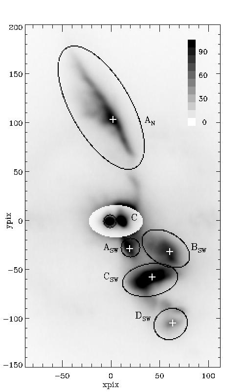
Figure 7: R Aqr observation from Oct. 11, 2014 in the N_Ha filter of the inner jet of R Aqr with cloud identification, astrometric points (defined for observations taken on Oct. 11, 2014), and used flux apertures. The red giant is located at $(x_{\rm pix},y_{\rm pix})=(0,0)$ and the pixel scale is 3.60 mas/pix.

The SW outer bubbles.

There is another group of lower surface brightness clouds in the SW at separations between $r_{\rm jet}\approx 0.8^{\prime\prime}-2.0^{\prime\prime}$. A variety of structures can be recognized; bubble-like structures E_SW, F_SW, elongated clouds G_SW, J_SW, and a shell-like structure including clouds H_SW and I_SW. The position of these clouds is confined to a wedge with an opening angle of about $\pm 15^{\circ}$ centered along a line with an orientation of about 230^∘ degrees.

The outer bubbles extend out to the extreme SW-corner of Fig. 6, which corresponds to a separation of $2.3^{\prime\prime}$ from the source. The off-axis field image OBS284_0038 extends the field of view out to $4^{\prime\prime}$ in a SW direction. Part of this outer field is shown in Fig. 8 demonstrating that there is no bright cloud outside Fig. 6. There is a very weak trace of a possible extended cloud at $r_{\rm jet}\approx 3.9^{\prime\prime}$, $\theta_{\rm jet}=230^{\circ}$, outside the region in Fig. 8, with a surface brightness $<0.003\leavevmode\nobreak\ {\rm ct/(s\,pix})$ significantly fainter than for H_SW, I_SW, or J_SW.

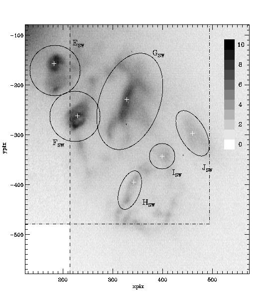
Figure 8: Images of the outer bubbles in the SW from Oct. 11, 2014 taken with the N_Ha-filter. The region on the right of the dashed line is from the off-axis field observation OBS284_0038 while the narrow section on the left is from the image shown in Fig. 6, which covers the region marked with the dashed dotted line. No data were taken for the lower left corner region. The red giant is located at $(x_{\rm pix},y_{\rm pix})=(0,0)$ and the pixel scale is 3.60 mas/pix.

The NE wisps.

Feature C_NE at $r_{\rm jet}=1.65^{\prime\prime}$ at a position angle of roughly $30^{\circ}$ is a $0.2^{\prime\prime}$ long, narrow, straight H$\alpha$ emission with an orientation perpendicular to the radial jet direction (Fig. 9). A second, weaker and shorter such wisp (B_NE) is seen at $r_{\rm jet}=1.2^{\prime\prime}$ with the same orientation indicating the possibility of a close relationship between these two features.

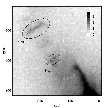
Figure 9: N_Ha-filter image of the NE-jet wisps. The image shows mean values for $3\times 3$ binned pixels in order to reduce the noise. The axis indicates the pixel coordinates for the unbinned frame where (0,0) is the coordinate of the red giant.

5.2 Positions for the H$\alpha$ clouds

The astrometric positions for the clouds for the points marked with a cross are given in Table 6 in polar coordinates $r_{\rm jet}$, $\theta_{\rm jet}$, where $r_{\rm jet}=0$ is the position of the central jet source $(x,y)={\rm(12.5\,pix,0.5\,pix)}$, and polar angles $\theta_{\rm jet}$ are measured from N over E. The “central” points of the clouds were defined by eye from the N_Ha observation shown in Fig. 6. The uncertainty of this procedure is about $\pm 1$ pixels ($\pm 3.6$ mas) for well defined (point-like) features (D_SW), about $\pm 2$ pixels for most clouds, and $\pm 4$ pixels for very elongated features like A_N or C_SW along the axis of elongation. These cloud positions are useful for the investigation of radial trends or for rough relative positions between H$\alpha$ clouds and features seen in other observations.

Temporal evolution of jet features.

Already from our two observing epochs separated by 60 days we see for certain well defined clouds a radial motion away from the jet source. We see also some changes in the brightness distributions for H$\alpha$ clouds close to the jet source $r_{\rm jet}<0.7^{\prime\prime}$ between August and October 2014. The inferred outward motion is about two pixels for the tangential wisp C_NE and about the same for the point-like cloud $D_{\rm SW}$. Thus, the motion is of the order of 40 mas/yr what corresponds to a projected gas velocity of roughly 40 km/s. Gas motions with this speed have been reported previously for the inner region $d<1^{\prime\prime}$ of the R Aqr jet (Mäkinen et al. 2004b). The famous R Aqr jet features A and B located at $r_{\rm jet}\;\hbox to0.0pt{\lower 2.5pt\hbox{$\sim$}\hss}\raise 1.5pt\hbox{$>$}\;4^{\prime\prime}$ move with an angular velocity of $0.2^{\prime\prime}$/yr or 200 km/s significantly faster, but they are located outside our field of view (e.g., Hollis et al. 1985; Kafatos et al. 1989; Mäkinen et al. 2004b) .

If we compare the ZIMPOL images with the HST observations of Paresce & Hack (1994) taken 23 year earlier, then we see hardly a correspondence in the location of the ionized clouds for $r_{\rm jet}<2^{\prime\prime}$. In 1991 the NE jet was brighter than the SW jet and the clouds in the NE were located at larger position angles between $35^{\circ}$ and 60^∘. In the SW there were only three jet clouds and it is not clear whether these clouds just faded away or moved out of the central jet region ($r_{\rm jet}<2^{\prime\prime}$) since 1991. The temporal evolution of the clouds for a detailed investigation of gas motions and flux variations will become much clearer from repeated measurements separated by several months to a few years. Therefore, we postpone a discussion until we have a better temporal coverage.

Table 6: Parameters of the jet clouds derived from the N_Ha (FW0) filter images from Oct. 11, 2014.

feature	position, size			aperture	H$\alpha$ surface brightness at $r_{\rm jet}$,$\theta_{\rm jet}$			H$\alpha$ aperture flux
	$r_{\rm jet}$	$\theta_{\rm jet}$	$\ell_{\rm cl}\times w_{\rm cl}$	$\ell_{\rm ap}\times w_{\rm ap}$	$sb_{\rm ct}({\rm N\_Ha})$	$sb_{\rm corr}$	${\rm SB}_{r,\theta}({\rm H}\alpha)$	$f_{\rm ct}$(N_Ha)	$ap_{\rm corr}$	$F_{\rm cl}({\rm H}\alpha)$
	[′′]	[∘]	[pix]	[pix]	ct/(s pix)		(b)	cts/s		(c)
jet source	0	–	$10\times 7$	$30\times 24$	47.6	$15:$	50700:	4550.	6.0	25.1
N / NE jet
AN	0.374	3.2	$70\times 15$:	$140\times 60$	2.57	4.3	785	2330	3.9	8.4
BNE	1.205	27.8	$30\times 10$:	$50\times 30$	0.030	6.0:	12.8	7.8	5.0	0.036
CNE	1.634	27.4	$60\times 10$	$100\times 50$	0.026	4.5:	8.3	25	4.3	0.099
SW inner jet
ASW	0.106	192.7	$12\times 10$:	$18\times 18$	0.98	13	905:	113	10	1.04
BSW	0.208	235.0	$30\times 20$	$52\times 32$	1.22	5.5	477	500	5.0	2.3
CSW	0.234	205.9	$37\times 16$	$56\times 32$	3.38	5.5	1320	1200	5.0	5.
DSW	0.420	203.1	$14\times 10$	$34\times 30$	0.88	$15:$	938	123	5.5	0.62
SW outer bubbles
ESW	0.833	225.1	$66\times 43$	$100\times 100$	0.108	4.0	30.7	193	3.8	0.68
FSW	1.225	217.5	$56\times 39$	$100\times 100$	0.12	4.1	35.3	202	3.8	0.71
GSW	1.405	232.0	$94\times 34$:	$200\times 120$	0.12	3.5:	28.6	419	3.5:	1.35
HSW	1.853	217.8	$30\times 20$	$80\times 40$	0.029	5.5	11.3	22.	4.5:	0.091
ISW	1.862	226.4	$24\times 24$	$50\times 50$	0.016	5.3	6.0	13.	4.5	0.054
JSW	1.935	234.4	$80\times 27$	$100\times 50$	0.019	4.0	5.4	32.	4.3	0.13
								$F_{\rm sum}$ (14 clouds)		46.1

5.3 Photometry for the H$\alpha$ clouds

The determination of flux parameters of individual H$\alpha$ features needs to take into account the instrument PSF and the size of the used synthetic photometric apertures. Therefore, the sizes of these apertures need to be tailored to the individual clouds and each feature requires its individual aperture correction. The PSF for ground-based, AO-assisted observations is highly variable (Section 2.4) and this needs also to be taken into account.

Thus, the measurement of H$\alpha$ cloud fluxes is complex and requires quite some effort. Depending on the scientific goal of a study, one might therefore evaluate the need for such measurements. Knowledge of the rough fluxes for the individual clouds in R Aqr is certainly useful for estimating cloud parameters. An uncertainty of a factor of two in the flux measurement introduces only an effect of a factor of $\approx 1.4$ for the determination of nebular density from cloud emissivities. Temporal line flux variations can be derived with a sensitivity of about 10 %, if fluxes are measured on a relative scale with respect to a suitable reference source in the image. In any case, the R Aqr commissioning “tests” presented here are an ideal data set to go through this H$\alpha$ flux calibration exercise, because we can check our results with the quasi-simultaneous H$\alpha$-data from HST.

Count rates.

For each cloud we define for the flux measurements synthetic round or elliptical apertures as shown in Figs. 7-9 with aperture sizes $\ell_{\rm ap}$ and $w_{\rm ap}$ given in Table 6. In most cases the center of the aperture ellipses is close but does not need to coincide with the astrometric point $r_{\rm jet}$ and $\theta_{\rm jet}$ of the cloud. The flux apertures are optimized to include cloud extensions and to exclude contributions from neighboring clouds, while the astrometric points pinpoint prominent features of the clouds.

The flux of an H$\alpha$ cloud $f_{\rm ct}({\rm N\_Ha})$ is calculated from the sum of background corrected count rates for all pixels in the aperture. The background level is the same for all pixels and it is equal to the mean values derived from all pixels in the plotted (one pixel wide) ellipses surrounding the synthetic aperture. This background accounts for all the diffuse flux from the measured cloud and the halos of all other H$\alpha$ emission features in the field. An alternative way to characterize H$\alpha$ cloud luminosities is via the surface brightness $sb_{\rm ct}{\rm(N\_Ha)}$ for the points $r_{\rm jet}$ and $\theta_{\rm jet}$ given in Table 6.

Measuring the aperture flux $f_{\rm ct}$ is accurate for strong, isolated, well defined clouds. For example if we compare the counts of the bright clouds A_N, B_SW, C_SW, E_SW , and F_SW taken in different H$\alpha$ filters (e.g., N_Ha and B_Ha) or different dates (August and October), then the count ratios for the individual clouds scatter about $\sigma=10$ % around the mean count ratio derived from all clouds. For faint clouds the scatter is about 20 %. These are good estimates of the flux measuring uncertainties which are most likely dominated by PSF variation effects.

Surface brightness measurements are also given in Table 6 because it seems that $sb_{\rm ct}$ is a more reliable measuring quantity for faint and diffuse clouds, but less reliable for compact or unresolved sources, because of peak flux variations due to changes in the AO performance. The above obtained scatter of $\sigma\approx 10$ % for cloud fluxes relative to a mean value indicates that flux variation at this level can be recognized in repeated data, if one emission component can be used as flux reference.

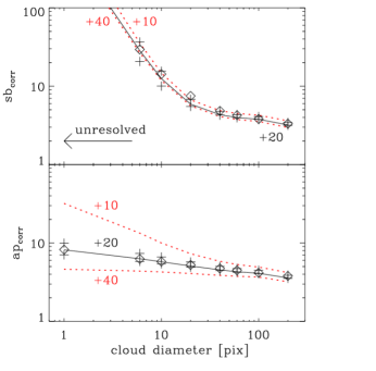
Figure 10: Simulated correction factors for R Aqr H$\alpha$ surface brightness $sb_{\rm corr}$ (upper) and aperture flux $ap_{\rm corr}$ (lower) as function of cloud diameter $\oslash_{\rm cl}$ [pix] for different apertures and AO performance. The full lines are for round clouds and aperture diameters $\oslash_{\rm ap}=\oslash_{\rm cl}+20$ and “average” conditions, and crosses indicate results for good and bad atmospheric conditions. The red dotted lines show the result for small $\oslash_{\rm cl}+10$ or large apertures $\oslash_{\rm cl}+40$. Results for elliptical model clouds with the same surface area but a ratio $l:b=4$ are plotted with diamonds

Background and aperture corrections.

In the next step, we simulate the effect of the extended PSF on the surface brightness and the cloud flux measurements. For this we simulate round and elliptical model clouds with constant surface brightness, the same total flux, but different diameters. These model clouds are convolved with the mean PSF for the CntHa filter (OBS284_0051-54), but also with the best (max) and worst (min) PSF (see Table 2 and Fig. 3). Then, the net surface brightness and net cloud fluxes are calculated for different apertures sizes like for the R Aqr H$\alpha$ data. The measured ratio between the initial model and PSF convolved cloud for surface brightness or cloud flux yields then the correction factors, $sb_{\rm corr}=sb_{\rm mod}/sb_{\rm PSF}$ and $ap_{\rm corr}=ap_{\rm mod}/ap_{\rm PSF}$ respectively, as function of model parameters. Figure 10 illustrates these model dependencies of $sb_{\rm corr}$ and $ap_{\rm corr}$ and Table 7 gives numerical values.

The central surface brightness is obviously strongly underestimated for measurements of unresolved and small clouds with diameters $\oslash_{\rm cl}<10$ pix. The correction factor $sb_{\rm corr}$ changes much less for extended sources $\oslash_{\rm cl}>20$ pix, and it depends only slightly on the diameter $\oslash_{\rm bck}=\oslash_{\rm cl}+10\leavevmode\nobreak\ {\rm pix}$, +20 pix (default), and +40 pix, of the ring or ellipse used for the background definition. In general, larger diameters yield a slightly lower background level and therefore a slightly higher net surface brightness requiring a slightly smaller correction factor $sb_{\rm corr}$.

The aperture correction $ap_{\rm corr}$ for the cloud flux depends quite strongly on the aperture size (see Fig. 10 and Table 7). For point sources the correction factor is small ($ap_{\rm corr}=4.63$) for large apertures and large ($ap_{\rm corr}=31.9$) for small apertures (see Table 7) because less halo flux is included in the aperture in the latter case. For extended clouds the aperture size dependence diminishes. The impact of the PSF quality is noticeable but not very dramatic.

Table 7: Simulation of correction factors for the surface brightness $sb_{\rm corr}$ and aperture photometry $ap_{\rm corr}$ as function of cloud diameter $\oslash_{\rm cl}$ [pix] calculated for the R Aqr CntHa PSF from Oct. 11, 2014.

$\oslash_{\rm cl}$		$sb_{\rm corr}$		$ap_{\rm corr}$
	$\oslash_{\rm bck}$=	$\oslash_{\rm cl}$+20	$\oslash_{\rm ap}$=	$\oslash_{\rm cl}$+10	$\oslash_{\rm cl}$+20	$\oslash_{\rm cl}$+40
$<1$		$>1000$		31.9	8.20	4.63
6		28.5		13.4	6.30	4.38
10		12.5		10.0	5.76	4.27
20		5.90		7.29	5.08	4.08
40		4.33		5.83	4.54	3.86
60		3.98		5.30	4.29	3.76
100		3.78		4.92	4.11	3.68
200		3.20		4.20	3.58	3.20

The simulated correction factors can be applied to the count rates per pixels $sb_{\rm ct}$ and the aperture count rates $f_{\rm ct}$ of the individual H$\alpha$ clouds. For this, we calculate for each cloud the average cloud diameter $\oslash_{\rm cl}=(\ell_{\rm cl}\cdot w_{\rm cl})^{1/2}$ and the average aperture diameter $\oslash_{\rm ap}=(\ell_{\rm ap}\cdot w_{\rm ap})^{1/2}$ and determine the applicable correction factors $sb_{\rm corr}$ and $ap_{\rm corr}$ from the simulation results in Fig. 10 and Table 7. The derived correction factors are given in Table 6.

The estimated uncertainty in the determination of the correction factors $sb_{\rm corr}$ and $ap_{\rm corr}$ is about $\pm 20\leavevmode\nobreak\ \%$ typically. The uncertainty is significantly larger for the surface brightness determination of marginally resolved clouds $\oslash_{\rm cl}<10$ pix because of the strong dependence of $sb_{\rm corr}$ with $\oslash_{\rm cl}$.

Surface brightness and flux for the H$\alpha$ clouds.

The resulting H$\alpha$ cloud fluxes $F({\rm H}\alpha)$ and surface brightness fluxes SB$({\rm H}\alpha)$ in Table 6 are then calculated from the measurements $f_{\rm ct}$, $sb_{\rm ct}$ and the derived corrections factors $ap_{\rm corr}$ and $sb_{\rm corr}$. These cloud fluxes are an important measuring result of the presented observations.

The conversion from corrected count rates into fluxes is given by Eq. 4 (using $c_{\rm zp}^{\ell}({\rm N\_Ha})=8.4\cdot 10^{-16}{\rm erg}\,{\rm cm}^{-2}{\rm ct}^{-1}$, ${\rm am}\cdot k_{1}=0.10$, and $m_{\rm mode}=0$). This yields the surface brightness flux per $3.6\times 3.6$ mas pixel and with ${\rm pix/arcsec}^{2}=77160$ the surface brightness SB(H$\alpha$) per arcsec.²

The central jet source has a flux of about $25\cdot 10^{-12}{\rm erg}\,{\rm cm}^{-2}{\rm s}^{-1}$, which is about 55 % of the total flux from the central region. The sum of all H$\alpha$ clouds is $F({\rm H}\alpha)=46\cdot 10^{-12}{\rm erg}\,{\rm cm}^{-2}{\rm s}^{-1}$ in agreement with the total flux derived in Sect. 4.2 for the central $3.6^{\prime\prime}\times 3.6^{\prime\prime}$ region of R Aqr. This is a reasonable result indicating that the 14 individual apertures miss perhaps 10 % or less of the H$\alpha$-emission in the central region, which originates from faint clouds and from diffuse emission. The polarimetric data, which will be presented in a future paper, show that there is diffuse H$\alpha$ emission because of dust scattering.

The interstellar extinction towards R Aqr is small because of the high galactic latitude of $b=-70^{\circ}$ and can be neglected for the interpretation of the measured cloud fluxes and surface brightnesses. However, circumstellar extinction is of course an issue, as the H$\alpha$ emission regions are embedded in a dust-rich stellar outflow.

5.4 The R Aqr jet in other ZIMPOL filters

5.4.1 [O I] and He I emission

Besides H$\alpha$, the jet of R Aqr is also clearly detected with SPHERE-ZIMPOL in the OI_630-filter and the He_I filter. Figure 11 shows the [O I] and He I observations for which the red giant was subtracted with scaled CntHa filter observations.

These difference images for [O I] and He I are of quite low quality because the emission is weak and the PSF from the CntHa observations is quite different when compared to the OI_630 and He_I data and therefore the subtraction residuals are large. A much better data quality for the [O I] and He I jet emission could be obtained with a dedicated strategy for subtracting the PSF of the bright red giant. Options, which are available for SPHERE-ZIMPOL observations, are (i) accurate PSF-calibration with a reference star observed with the same instrument configuration as R Aqr for a proper PSF subtraction, (ii) the combination of images taken with different field orientations to remove the instrumental (fixed) PSF features, or (iii) angular differential imaging with pupil stabilized observations which would be particularly powerful for detecting and measuring point-like emission from a weak companion. Simultaneous spectral differential imaging is not possible for the OI_630 and He_I filters (unlike for the H$\alpha$ filters), because they are located in the common beam before the ZIMPOL beam splitter and one filter “feeds” both ZIMPOL arms.

Nonetheless, the OI_630 and He_I filter data (Fig. 11) allow a useful qualitative description. Line emission of [O_I] is clearly detected for the cloud components A_N, the SW inner jet cloud C_SW and probably also B_SW, and the SW outer bubbles E_SW, F_SW, G_SW. The flux in these clouds is about ten times lower than the measured H$\alpha$ flux. An open issue with the OI_630 filter emission is the relative contribution of the [S_III] 631.2 nm line, which might be responsible for $\approx 10-50$ % of the emission in the OI_630 filter according to the R Aqr spectrum shown in Fig. 2.

He I emission is detected for the jet clouds A_N, C_SW, F_SW, G_SW and possibly there is also some emission in B_SW and E_SW (affected by a diffraction spike). The He I 587 nm emission is weaker by about a factor of two when compared to [O I] 630 nm.

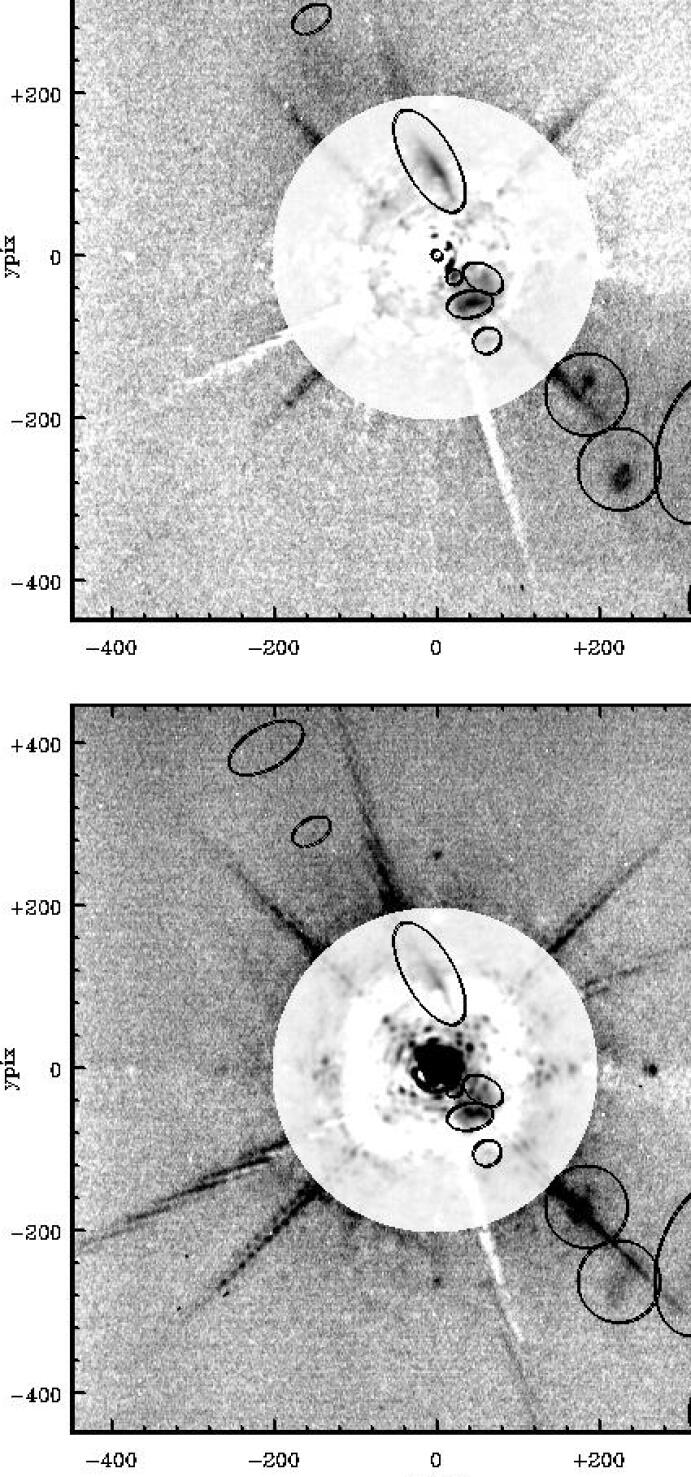
Figure 11: SPHERE-ZIMPOL OI_630- and HeI-filter observations of the R Aqr jet. The emission of the red giant is strongly reduced by subtracting a scaled CntHa filter image. The gray scale tables are multiplied by a factor of ten for the inner $r_{\rm RG}<0.72^{\prime\prime}$ region.

5.4.2 Emission from the central jet source

The central jet source is very bright in the H$\alpha$ emission. It is therefore of interest to search for emission in other filters or define at least upper flux limits.

Our simple test data, which were taken without dedicated PSF subtraction procedures, provide a flux contrast limit of about $F_{\rm jet}/F_{\rm RG}\approx 0.05$ between the central jet source and the red giant. We identify only for the V-band filter observation from October 11, 2014 a source at the location of the central jet source. The contrast is about $F_{\rm jet}/F_{\rm RG}\approx 0.10$ with an estimated uncertainty of $\pm 0.05$. This translates with red giant brightness of ${\rm V}=11.3^{m}$ (Table 3) into a continuum magnitude of $V_{\rm jet}\approx 14.0\,(\pm 0.7)^{m}$ for the jet source.

In all other filters no continuum emission is detected ($F_{\rm jet}/F_{\rm RG}\leq 0.05$) from the central jet source, neither for the He_I, OI_630 line filters, nor the V_S, Cnt_Ha, TiO_717, Cnt_748, and Cnt_820 intermediate band continuum filters. The resulting continuum magnitude limits are $m_{\rm jet}>m_{\rm RG}({\rm Tab.\leavevmode\nobreak\ \ref{PhotRAqr}})+3.25^{m}$ when taking the red giant magnitudes from Table 3.

The detection in the V-band yields, with the distance modulus of $m-M=6.7^{m}$ for R Aqr, an absolute magnitude of about $M_{\rm V}=7.3^{m}$. This is brighter than expected for a hot white dwarf on the cooling track and more compatible with a star of the heterogeneous class of O or B subdwarfs, which are mass accreting and “active” in interacting binary systems (e.g., Heber 2009). According to historical Korean nova records, the hot component could have had a nova like outburst in 1073 and 1074 (Yang et al. 2005). Thus, the hot star in R Aqr could be an accreting compact object on its evolutionary track from a symbiotic nova outburst towards a cold and less luminous white dwarf state (see Murset & Nussbaumer 1994).

The observations in the He_I and OI_630 line filters originate from August 2014, when the red giant was about one magnitude brighter than in October 2014. We can define line flux limits relative to H$\alpha$, but they are with $F({\rm He\leavevmode\nobreak\ I})/F({\rm H}\alpha)<0.15$ and $F([{\rm O\leavevmode\nobreak\ I}])/F({\rm H}\alpha)<0.15$ not sensitive. These limits are compatible with the expected line emission from an ionized gas nebula.

With ZIMPOL / SPHERE high contrast observations, using, for example, pupil stabilized angular differential imaging, it should be possible to reach a contrast limit of about 5 mag between the red giant and the jet source for the current angular separation, or line flux ratios $<0.05$ (relative to H$\alpha$). Thus, a better characterization of the jet source is certainly possible if dedicated observations are carried out during the luminosity minimum of R Aqr.

6 HST line filter observations

6.1 HST / WFC3 Data

R Aqr was also observed in 2013 and 2014 with the Ultraviolet-Visible (UVIS) channel of the HST Wide Field Camera 3 (WFC3). Long and short exposures were taken in the four line filters F502N, F631N, F656N, and F658N targeting the nebular emission lines [O III] 500.7 nm, [O I] 630.0 nm, H$\alpha$ 656.3 nm, and [N II] 658.3 nm. Exposures with “long” integration times of either 1086 s or 2085 s are saturated in the center, but they show the extended jet and nebulosity at $r>1^{\prime\prime}$ with very high sensitivity as shown for H$\alpha$ in Fig. 1a. The “short” exposures with $t_{\rm exp}$ between 15 s and 70 s are not saturated and such data were taken in all four filters on October 18, 2014 only seven days after our observation from October 11. Therefore, the HST data complement in an ideal way our SPHERE-ZIMPOL observations with additional, quasi-simultaneous line measurements for [O III] and [N II], and higher sensitivity H$\alpha$ and [O I] images. The HST provides high quality flux calibrations which is particularly important for a cross check of our ZIMPOL H$\alpha$ flux measurement and calibration procedure.

Table 8 lists the parameters for the unsaturated HST data selected for this work. The spatial resolution of HST-UVIS is about 78 mas (two pixels). We consider only the central R Aqr region of about $3.5^{\prime\prime}\times 3.5^{\prime\prime}$ or $90\times 90$ pixels which is shown in Fig. 12 for H$\alpha$, [O III], and [O I]. Of course, the entire HST field of view contains a lot of important information about the outer jet and nebula of R Aqr, but this is beyond the scope of this paper.

Table 8: HST WFC3 observations of R Aqr from Oct. 18, 2014 used for this work.

filter	F502N	F631N	F656N	F658N
ident “ic9k0…”	6vnq	7vwq	6010	7010
$t_{\rm exp}$	50 s	24 s	70 s	70 s
$\lambda_{c}$ [nm]	501.0	630.4	656.3	658.5
$\Delta\lambda$ [nm]	6.5	5.8	1.8	2.8
Transm. $T$	0.230	0.230	0.228	0.245
target line	[O III]	[O I]	H$\alpha$	[N II]
other line	-	[S III]	[N II]	H$\alpha$

For our analysis we started with the pipeline processed images as they can be retrieved from the HST-MAST archive. In the innermost R Aqr region, the same H$\alpha$ cloud structures can be recognized as in the ZIMPOL H$\alpha$ images. Because of the lower resolution of the HST data, the clouds A_SW and D_SW cannot be resolved and the clouds B_SW and C_SW are merged into one single feature, which we call (B+C)_SW.

6.2 Line flux measurements for the HST data

The HST observations of R Aqr taken with the H$\alpha$, [O III], [N II], and [O I] line filters show quite significant differences for the innermost clouds (see Fig. 12). The strongest emission in the red filters F631N, F656N, and F658N originates from the central, unresolved stellar binary. Interestingly, the stellar binary is rather weak in the [O III] line, weaker than the clouds A_N and (B+C)_SW, indicating that the [O III]/H$\alpha$ ratio varies strongly between stellar binary and jet clouds. The jet clouds are much fainter in [O I] than in H$\alpha$ confirming the result from SPHERE / ZIMPOL, and also the [N II] line is much weaker than H$\alpha$ or [O III] (see Table 9).

For the line flux measurements and the comparison with the ZIMPOL data, we have selected six well defined emission features in the HST data which are indicated with elliptical apertures in Fig. 12. These are the stellar binary SB, and the clouds A_N, (B+C)_SW, E_SW, F_SW, and G_SW as defined in the ZIMPOL H$\alpha$ observations.

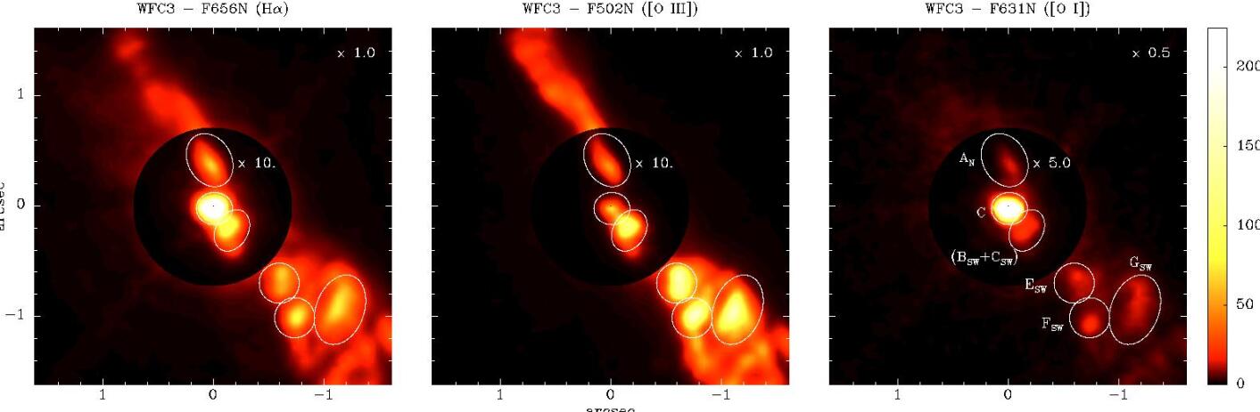
Figure 12: HST images of the central region of R Aqr taken in the H$\alpha$, [O III], and [O I] filters. The color scale of the inner region is ten times larger than the outer region and factors for the application of the color scale are indicated. The cloud features are identified in the O I panel.

The apertures for the flux measurements were chosen to be similar to the used ZIMPOL cloud apertures, if possible. For this, each $39.6\times 39.6$ mas pixel of the HST image was expanded into $11\times 11$ pixels with a size of $3.6\times 3.6$ mas with a flux conserving interpolation. The expanded images, which are actually displayed in Fig. 12 together with the flux apertures, have the pixel scale of the ZIMPOL data so that the same type of measuring routines could be used.

The resulting line fluxes are given in Table 9. Fluxes were calculated from the summed count rates ct/s (called e^-/s in the HST jargon) in a given cloud aperture using the transformation

$$F_{\rm cl}={\rm ct/s}\cdot\,{1\over A\cdot T}\,{hc\over\lambda}\cdot c_{\rm ap}\,,$$

where $A=45239\leavevmode\nobreak\ {\rm cm}^{2}$ is the effective HST primary mirror area, $T$ the HST-WFC3 system transmission, $hc/\lambda$ the line photon energy, and $c_{\rm ap}$ the aperture correction for a given cloud. For each filter $T$ is listed in Table 8 and as derived from the transmission curves given in the WFC3 handbook.

The aperture corrections $c_{\rm ap}$ are estimated as for the ZIMPOL data (see Sect. 5.3) by calculating the halo (or background) corrected energy within given apertures for simple models of extended clouds, convolved with the HST point spread function. The derived $c_{\rm ap}$-values listed in Table 9 for the different clouds are quite large, because small apertures must be used to avoid an overlap with neighboring clouds. The $c_{\rm ap}$ correction factors introduce an estimated uncertainty of about $\pm 10-20$ % and this dominates the errors in the line fluxes given in Table 9.

Line flux ratios, for example, $F({\rm[O\leavevmode\nobreak\ III]})/F({\rm H}\alpha)$, from HST are expected to be very accurate ($\pm 10\leavevmode\nobreak\ \%$), because systematic line measuring errors, for example, due to the $c_{\rm ap}$ correction factors, are strongly reduced for line ratios. However, one should also note that the emission regions for different lines do not coincide always because of the complex substructure of a cloud. For example the clouds F_SW and G_SW show different structures for [O III] and [O I] (see Fig. 12).

HST line fluxes for the central jet source.

The mira variable and the central jet source are not resolved in the HST data. Therefore we need to correct for the determination of the line flux for the central jet source the contribution of the red giant to the flux in the SB-aperture.

Table 9 gives a value “SB total” which would corresponds to the line flux from the region covered by the central stellar binary (SB) aperture assuming that all photons emitted from this region are line photons. This is certainly not true, because the contribution from the red giant continuum is at least for the red line filters substantial. The following line gives an estimate for the relative contribution of the red giant to the flux in the SB aperture as discussed in the following paragraphs and the third line is then the resulting line flux estimate for the central jet source, if the contribution of the red giant is taken into account.

For H$\alpha$ and [O I], the contribution of the red giant can be estimated from the ZIMPOL observations from which we measured for October 11 a relative photon ratio of 1.1$\pm 0.1$ between the jet source and the red giant in the N_Ha filter. The H$\alpha$ filter F656N of HST has twice the width of the ZIMPOL N_Ha filter and therefore the contribution of the red giant is roughly 65 % of the total flux in the SB-aperture in the H$\alpha$ HST image.

The [O I] line was not detected for the central jet source with the ZIMPOL on August 12. The estimated contrast limit is [O I]/RG $<0.05$, which turns into a contrast limit of about $<0.1$ for the October 18 HST epoch when the red giant was fainter. The [O I] filters in ZIMPOL and HST have roughly the same widths and one can assume as a conservative limit that less than 20 % of “SB total” value for the F603N filter for the SB aperture originates from nebular line emission.

For [N II] a similar red giant continuum flux as for the H$\alpha$ filter can be assumed. This yields an expected photon count rate for the red giant in the F658N filter which is slightly above the measured count rates. Thus, the [N II] emission line flux is low and a conservative line flux limit is indicated in Table 9.

The contribution of the red giant in the F501N filter is unclear and difficult to estimate. Therefore, we use as a conservative upper limit for the [O III] line flux the “SB total” line flux.

Table 9: HST emission line fluxes for R Aqr emission clouds derived from the H$\alpha$, [O III], [N II] and [O I] filter observations.

cloud	$c_{\rm ap}$	H$\alpha$	[O III]	[N II]	[O I]
AN	1.4	5.5	4.8	0.51	0.60
(B+C)SW	1.9	5.1	10.0	0.25	$<0.5$
ESW	1.8	0.41	1.8	0.030	$<0.1$
FSW	1.8	0.54	1.5	0.11	0.046
GSW	1.4	0.89	2.2	0.35	0.42
central jet source
SB total	2.0	$34$	$2.6$	$16$	$15$
rel. RG cont.		$\approx 65\leavevmode\nobreak\ \%$	unclear	$>80\leavevmode\nobreak\ \%$	$>80\leavevmode\nobreak\ \%$
C (jet source)		$\approx 12$	$<2.6$	$<3$	$<3$

H$\alpha$ flux comparison between HST and ZIMPOL.

We can now compare the derived H$\alpha$ cloud fluxes derived in Table 9 for the HST observation with Table 6 derived from the ZIMPOL observations. The obtained mean H$\alpha$ flux ratio is $F_{\rm HST}/F_{\rm ZIMPOL}=0.67\pm 0.05$ for the five clouds $A_{\rm N}$, $(B+C)_{\rm SW}$, $E_{\rm SW}$, $F_{\rm SW}$, $G_{\rm SW}$. This is quite a significant difference. However, the relative scatter of $\sigma/{\rm mean}\approx 7.5\leavevmode\nobreak\ \%$ in the derived flux ratios $F_{\rm HST}/F_{\rm ZIMPOL}$ for the five clouds is very small. Thus, we can conclude that the H$\alpha$ flux ratios between individual clouds, like $F(E_{\rm SW})/F(A_{\rm N})$ , agree very well between HST and ZIMPOL-SPHERE.

The large overall H$\alpha$ flux difference is hard to explain. The main uncertainties are the aperture correction factors derived for the ZIMPOL measurements and the preliminary flux zero-points calibration of ZIMPOL, which is not well established yet. More investigation is required to clarify this issue.

7 Physical parameters for the H$\alpha$ clouds

7.1 Temperatures and densities for the jet clouds

In this section we derive nebular densities $N_{e}$ and temperatures $T_{e}$ for the jet clouds from the measured ZIMPOL H$\alpha$ line emissivities $\epsilon({\rm H}\alpha)$ and the HST [O III]/H$\alpha$ line ratios. The H$\alpha$ emissivity provides a good measure of the nebular density, and the combination with the [O III]/H$\alpha$ ratio yields the nebular temperature.

For the theoretical line emissivities $\epsilon({\rm H}\alpha),$ we assume that the H$\alpha$ line is produced mainly by case B recombination (Osterbrock & Ferland 2006; Hummer & Storey 1987). Case B assumes that the lower H I Lyman lines are optically thick for the jet clouds in R Aqr which corresponds to H I column densities of roughly $\;\hbox to0.0pt{\lower 2.5pt\hbox{$\sim$}\hss}\raise 1.5pt\hbox{$>$}\;10^{14}\,{\rm cm}^{-2}$. Case B conditions might not be fulfilled because the emission clouds in R Aqr are small ($r\approx 10^{14}$ cm), and there is significant line broadening due to gas motions $v>100$ km/s so that Lyman line photons may escape. Thus, case A (optical thin Lyman lines) might apply and the corresponding recombination emissivities would be lower by a factor of about 0.67.

On the other side, there could be an enhancement of the H$\alpha$ line emissivities by collisions from the ground state or the metastable state H I ²S. Collisions from the ground state are important for high nebular temperatures ($T>10000$ K) near a shock front (see, e.g., Raymond 1979; Hartigan et al. 1987; Raga et al. 2015a) but this effect can be strongly suppressed if X-rays from the shock reduce strongly the density of H⁰ by photo-ionization in that region. In shock models and observations of Herbig-Haro objects, most of the H$\alpha$ emission originates from recombination in the cold ($T_{e}\;\hbox to0.0pt{\lower 2.5pt\hbox{$\sim$}\hss}\raise 1.5pt\hbox{$<$}\;10000$ K) post-shock cooling region (e.g., Raymond 1979; Raga et al. 2015b). In R Aqr the nebular densities in the innermost jet region are of the order $10^{6}\,{\rm cm}^{-3}$, which is at least two orders of magnitude higher when compared to typical Herbig-Haro objects. For R Aqr several studies on the jet emission exist (Burgarella et al. 1992; Kellogg et al. 2007; Nichols & Slavin 2009) for line emitting clouds located at large separations $>1000$ AU, several times further out than the clouds studied in this work. There the conditions are comparable to Herbig-Haro objects with $T_{e}\approx 10^{4}$ K, $N_{e}\approx 10^{4}{\rm cm}^{-3}$ will the X-ray emitting material has parameters of $T_{e}\approx 10^{6}$ K and $N_{e}\approx 10^{2}{\rm cm}^{-3}$.

The line emission of the central nebula of R Aqr was investigated by Contini & Formiggini (2003) with a (plane parallel) shock model describing a scenario where a fast (preionized) wind from the hot component with $v=110$ – $125$ km/s and a high pre-shock density of $6\cdot 10^{4}{\rm cm}^{-3}$ collides with the wind of the red giant. They obtain for the main emission region (post-shock cooling region) a temperature of $T_{e}\approx 10^{4}$ K and a density of $\geq 6\cdot 10^{5}{\rm cm}^{-3}$. This indicates that the resulting H$\alpha$-emission in the jet clouds imaged by us originates mainly from recombination.

For these reason it seems reasonable to adopt the case B recombination emissivities as first approximations for the “theoretical” H$\alpha$ emissivities for our study of R Aqr, but considering the complexity of the H$\alpha$ line formation we admit an uncertainty of a factor of two in $\epsilon_{\rm th}({\rm H}\alpha)$. The impact on the determination of the nebular density is then about an uncertainty of a factor of 1.4.

The adopted “theoretical” H$\alpha$ emissivity is

$$\epsilon_{\rm th}({\rm H}\alpha)=\alpha_{B}({\rm H}\alpha,T_{e})\,h\nu\,N_{p}N_{e}\,,$$ (5)

where $\alpha_{B}({\rm H}\alpha,T_{e})\approx 7.86\cdot 10^{-14}\,{\rm cm}^{3}{\rm s}^{-1}\cdot(T_{e}/10000\leavevmode\nobreak\ {\rm K})^{-0.9}$ are the case B recombination coefficients for the H$\alpha$ line, $T_{e}$ the electron temperature, $h$ the Planck constant, $\nu$ the photon frequency, and $N_{p},N_{e}$ the proton and electron densities (see Osterbrock & Ferland 2006). We approximate $N_{p}\approx N_{e}$, assuming that the jet clouds are strongly ionized.

Averaged H$\alpha$ emissivities $\langle\epsilon({\rm H}\alpha)\rangle$ for a given cloud can be derived from the observed line flux $F({\rm H}\alpha)$, the distance $d$ to R Aqr, and the cloud volume $V_{\rm cl}$ estimated from the measured cloud size

$$\langle\epsilon({\rm H}\alpha)\rangle\approx{4\pi d^{2}F({\rm H}\alpha)\over V_{\rm cl}}\,.$$ (6)

The cloud volume is calculated according to $V_{\rm cl}=\pi\,(\ell_{\rm cl}\cdot w_{\rm cl})^{3/2}/6$, where cloud lengths $\ell_{\rm cl}$ and widths $w_{\rm cl}$ are taken from Table 6. This assumes a cloud diameter along the line of sight which is equivalent to $s_{\rm cl}\approx(\ell_{\rm cl}\cdot w_{\rm cl})^{1/2}$. Thus, we define $\oslash_{\rm cl}=(\ell_{\rm cl}\cdot w_{\rm cl})^{1/2}$ as the equivalent diameter for a spherical cloud with the same volume. This approximation would introduce a bias if the H$\alpha$-clouds in R Aqr have typically filamentary or strongly flattened structures.

An alternative determination of $\langle\epsilon({\rm H}\alpha)\rangle$ can be made from the measured surface brightness SB(H$\alpha$) using the relation

$$\langle\epsilon({\rm H}\alpha)\rangle\approx{\Omega\over 4\pi}{{\rm SB}({\rm H}\alpha)\over s_{\rm cl}}\,.$$ (7)

For the SB-values from Table 6, which are given per arcsec², one must use $\Omega/4\pi=1.87\cdot 10^{-12}$. As above, we use $s_{\rm cl}\approx\oslash_{\rm cl}$ for the line of sight diameter of a given cloud.

Table 10 lists the resulting emissivities $\langle\epsilon({\rm H}\alpha)\rangle$ using the cloud flux $F_{\rm cl}$ or surface brightness SB_cl data from Table 6. Both methods yield similar results $\epsilon_{F}/\epsilon_{\rm SB}\approx 1.4$ with a scatter of 0.15 dex. We select for well defined bright clouds the emissivities derived from $F_{\rm cl}$ and for diffuse and faint clouds the values from SB_cl, because these values seem to be less affected by background determination or aperture definition uncertainties. The obtained emissivities indicate nebular densities in the range $N_{e}\approx 10^{5}-10^{8}\,{\rm cm}^{-3}$ for the clouds $r_{\rm jet}<2^{\prime\prime}$ ($<400$ AU) of the R Aqr jet.

The nebular temperature can be constrained by the [O III]/H$\alpha$ line ratio derived from the HST data. The [O III] 500.6 nm line is a collisionally excited line and its emissivity is described by

$$\epsilon({\rm[O\leavevmode\nobreak\ III]})=N_{u}\,h\nu\,A_{ul}=N_{{\rm O}^{+2}}\,h\nu\,A_{ul}\,{N_{e}q_{lu}\over A_{ul}+N_{e}q_{ul}}\,,$$ (8)

where $N_{u}$ is the density of O⁺²-atoms in the upper state (¹D) of the [OIII] 500.7 nm transition, $h\nu=hc/\lambda$ the corresponding photon energy, and $A_{ul}$ the transition rate of the line. The level population $N_{u}$ is defined by the balance of collisional excitations $N_{e}q_{lu}$ from the lower states (ground level term), and the collisional de-excitations $N_{e}q_{ul}$ and radiative decays $A_{\rm ul}$ (Osterbrock & Ferland 2006). The [O III] emissivity is very sensitive to the temperature because of the exponential temperature term in the collisional excitation $q_{lu}\propto{\rm exp}(-h\nu/kT_{e})$.

For low density gas the emissivity of collisionally excited lines is $\epsilon\propto N_{{\rm O}^{+2}}N_{e}$ or proportional to the density squared. However, the central clouds in R Aqr are very dense, above the critical density of the [OIII] 500.7 nm transition, and therefore collisional de-excitations are very important for $A_{ul}\ll N_{e}q_{ul}$. In this high density regime, the emissivity is $\epsilon({\rm[O\leavevmode\nobreak\ III]})\propto N_{{\rm O}^{+2}}{\rm exp}(-h\nu/kT_{e})$ or proportional to the density of the O⁺² atoms.

We can relate $N_{{\rm O}^{+2}}$ to the electron density $N_{e}$ with the approximation

$$N_{{\rm O}^{+2}}={N_{{\rm O}^{+2}}\over N_{\rm O}}{N_{\rm O}\over N_{\rm H}}{N_{\rm H}\over N_{e}}\,N_{e}\approx 5\cdot 10^{-4}\,N_{e}\,.$$

This assumes for the clouds that hydrogen is strongly ionized $(N_{\rm H}/N_{e}\approx 1)$, oxygen is predominantly in the form O⁺² ($N_{{\rm O}^{+2}}/N_{\rm O}\approx 1$), and the relative abundance of oxygen to hydrogen is solar $N_{\rm O}/N_{\rm H}=5\cdot 10^{-4}$. All clouds for which we have measured line fluxes from the HST data (Table 9) show much stronger [O III] than [O I] or [N II] lines, what supports the assumption of a high degree of ionization.

A diagnostic diagram for the determination of nebular densities and temperatures from the ZIMPOL H$\alpha$ emissivities $\langle\epsilon({\rm H}\alpha)\rangle$ and the $F([{\rm O\leavevmode\nobreak\ III}])/F({\rm H}\alpha)$ line ratios from HST is plotted in Fig. 13 for the clouds with HST line flux measurements. The diagram is based on simple theoretical line emissivities described above (Eqs. 5 and 8) using the atomic data compiled in Osterbrock & Ferland (2006), and adopting a solar abundance ${N_{{\rm O}^{+2}}/N_{e}}=5\cdot 10^{-4}$.

The considered clouds show a range of about a factor of 100 in density from about $N_{e}\approx 3\cdot 10^{5}{\rm cm}^{-3}$ to $3\cdot 10^{7}{\rm cm}^{-3}$, while the derived temperatures are between about $T_{e}=10^{\prime}000$ K and $20^{\prime}000$ K. Because of the collisional de-excitation of the nebular [O III]-line, the $F([{\rm O\leavevmode\nobreak\ III}])/F({\rm H}\alpha)$ line ratio decreases rapidly for increasing density. A high density can therefore naturally explain the weak [OIII]-emission from the central jet source.

Figure 13: Diagnostic diagram based on H$\alpha$ line emissivities $\epsilon({\rm H}\alpha)$ and [O III]/H$\alpha$ line ratios assuming an abundance ratio $N_{{\rm O}^{+}}/N_{{\rm H}^{+}}=5\cdot 10^{-4}$. The crosses give the values for the H$\alpha$ clouds with [O III]/H$\alpha$-ratios from HST.

We can assume, based on Fig. 13, that all the H$\alpha$-clouds in Table 10 have a temperature of roughly $T_{e}\approx 15000\pm 5000$ K. Adopting this value for clouds without [O III]/H$\alpha$ ratio yields densities for all these clouds.

Table 10: Parameters for the H$\alpha$ clouds in the jet of R Aqr for Oct. 11, 2014.

cloud	$r_{\rm RG}$	$\oslash_{\rm cl}$	method	$\epsilon(H\alpha)$	$F$-ratio	$T_{e}$	$N_{e}$	$M_{\rm cl}$
	$10^{13}$ [cm]	$10^{13}$ [cm]	$F/{\rm SB}$	$10^{-12}{\rm erg/cm}^{-3}$	[O III]/H$\alpha$	[K]	$10^{6}{\rm cm}^{-3}$	[10-9M⊙]
C (center)	14.3	9.8	$F_{\rm cl}$	288	$<0.2$	20 000	44	24.
N / NE jet
AN	121	38	$F_{\rm cl}$	1.7	0.87	13 000	2.9	91.
BNE	385	20	${\rm SB}_{\rm cl}$	0.034			0.43	2.1
CNE	525	29	${\rm SB}_{\rm cl}$	0.015			0.29	4.0
SW inner jet
ASW	41.5	13	$F_{\rm cl}$	5.3			5.4	6.6
BSW	82.1	29	$F_{\rm cl}$	1.05	2.0a	20 000	2.7	36.
CSW	85.0	29	$F_{\rm cl}$	2.6	2.0a	20 000	4.1	56.
DSW	144	14	$F_{\rm cl}$	2.5			3.8	5.8
SW outer bubbles
ESW	283	63	$F_{\rm cl}$	0.030	4.4	13 000	0.39	54.
FSW	410	55	$F_{\rm cl}$	0.046	2.8	11 000	0.46	43.
GSW	471	66	$F_{\rm cl}$	0.021	2.5	10 000	0.46	77.
HSW	614	29	${\rm SB}_{\rm cl}$	0.026			0.34	4.7
ISW	619	29	${\rm SB}_{\rm cl}$	0.011			0.25	3.2
JSW	644	55	${\rm SB}_{\rm cl}$	0.0053			0.17	16.
uncert.		$\pm 0.05$ dex		$\pm 0.25$ dex	$\pm 0.05$ dex		$\pm 0.30$ dex	$\pm 0.45$ dex

7.2 Cloud density versus cloud distance

The H$\alpha$ clouds in the inner jet region of R Aqr show a systematic decrease in surface brightness and cloud flux with distance from the central jet source (e.g., Fig. 6). This points to a relation between distance and cloud density, because the emissivity is $\epsilon({\rm H})\propto N_{e}^{2}$.

Figure 14 shows the cloud parameters from Table 10 in the distance - density plot and the points are well fitted with a power law $N_{e}=N_{14}\,r_{\rm RG}^{-1.3}$ with the normalization density $N_{14}=6\cdot 10^{7}{\rm cm}^{-3}$ at the distance $r_{\rm RG}=10^{14}{\rm cm}$. Essentially the same correlation is found if the point for the central jet source at $r_{\rm RG}=1.49\cdot 10^{14}{\rm cm}$ is not considered for the least square fit, or if the density is plotted versus jet source distance $r_{\rm jet}$ instead of $r_{\rm RG}$ (omitting the jet source).

The tight correlation between density $N_{e}$ and cloud distance from the red giant $r_{\rm RG}$ is indicative of a kind of pressure equilibrium between the neutral gas of the red giant wind and the ionized H$\alpha$ clouds in the jet. The molecular hydrogen density $N_{{\rm H}_{2}}$ in an isothermal spherical wind from the red giant can be estimated from the formula $N_{{\rm H}_{2}}(r)=\dot{M}/(4\pi\,\mu\cdot m_{\rm H}\,v_{\infty}r^{2})$, where we adopt $\mu=2$ for the mean atomic weight of the particles, and $m_{\rm H}$ is the mass of the hydrogen atom. Figure 14 includes the lines for the expected $N_{{\rm H}_{2}}(r)$ density dependence, if the mira has a spherical mass loss of $\dot{M}_{\rm RG}=10^{-5}$ or $10^{-6}\,{\rm M}_{\odot}/{\rm yr}$ and a wind velocity of $v_{\infty}=10\leavevmode\nobreak\ {\rm km/s}$. Unfortunately, the mass loss rate for the mira variable in R Aqr is not well known and literature values range from about $\dot{M}_{\rm RG}=10^{-7}\,{\rm M}_{\odot}/{\rm yr}$ to $10^{-5}\,{\rm M}_{\odot}/{\rm yr}$ (e.g., Mayer et al. 2013; Bujarrabal et al. 2010).

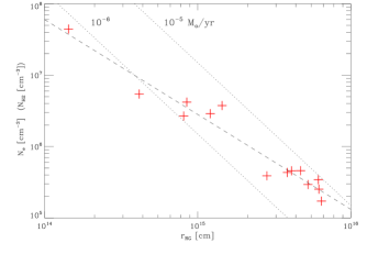
Figure 14: H$\alpha$ cloud densities $N_{e}$ as function of distance to the red giant $r_{\rm RG}$. The dashed line is the power law fit $N_{e}\propto r_{\rm RG}^{-1.3}$ to the derived values. The dotted lines illustrate the expected molecular hydrogen density $N_{{\rm H}_{2}}(r_{\rm RG})$ in the red giant wind for a wind velocity of $v_{\infty}=10$ km/s and mass loss rates $\dot{M}=10^{-5}$ and $10^{-6}{\rm M}_{\odot}$/yr.

The general trend of decreasing cloud brightness, and therefore decreasing density, continues beyond the ZIMPOL field of view, as can be inferred from the HST WFC3 image (Fig. 1a). For example, the H$\alpha$ peak surface brightness of the bright, bow shaped jet clouds in the NE at a separation of $\approx 10^{\prime\prime}$ ($r_{\rm RG}\approx 3\cdot 10^{16}$) is about ten times lower than for the clouds H_SW, I_SW, J_SW in the ZIMPOL field, and the SB of all clouds located at even larger distances $>10^{\prime\prime}$ are of the order of 100 times lower.

Ionized mass and jet outflow limits.

Summing up the mass of the bright H$\alpha$ clouds and the central source listed in Table 10 yields a summed mass of about $M_{\Sigma{\rm cl}}=5\cdot 10^{-7}{\rm M}_{\odot}$. This can be compared with the expected molecular hydrogen gas in the red giant wind. If we assume a mass loss rate of $\dot{M}_{\rm RG}=10^{-6}\,{\rm M}_{\odot}$/yr and $v_{\infty}=10$ km/s or 2 AU/yr (10 mas/yr), then a spherical wind contains about $2\cdot 10^{-4}{\rm M}_{\odot}$ of H₂ from 10 to 400 AU. This is roughly the region covered by the field of view of ZIMPOL. Thus, the bright H$\alpha$ clouds in R Aqr contain only a small fraction of $0.1-1$ % of the circumstellar matter within 400 AU if $\dot{M}_{\rm RG}=10^{-6}{\rm M}_{\odot}$ is adopted.

The ionized gas in the 14 selected bright emission regions fills a volume of about $10^{5}$ AU, which is of the order of 0.03 % of the volume $V_{\rm 400AU}$ within $r_{\rm RG}=400$ AU from the star. All this ionized gas is localized in the two NE and SW jet cones with an opening angle of about $\theta\approx\pm 15^{\circ}$. These two cones are about $3\leavevmode\nobreak\ \%$ of the spherical volume $V_{\rm 400AU}$. Accordingly, only about 1 % of the volume in the adopted $\pm 15^{\circ}$ jet cones are bright clouds, the rest of the cone is filled with low emissivity gas.

We can estimate an upper limit for the low emissivity gas which could be present in the two jet cones. The sensitivity of the ZIMPOL images is quite limited because of the extended AO-PSF. Ionized gas with the same temperature but with ten times lower density (100 times lower emissivity) than the considered 14 bright H$\alpha$ jet clouds could fill the two jet cones without being detected in the ZIMPOL image. But, the sensitive H$\alpha$ and [O III] HST images (Fig. 12) show faint emission along the two jet cones and this could originate from such low density gas. This ionized low density gas ($T_{e}\approx 15\,000\leavevmode\nobreak\$K) could contain up to ten times more mass than the bright H$\alpha$ clouds or up to $M_{{\rm H}\alpha}\;\hbox to0.0pt{\lower 2.5pt\hbox{$\sim$}\hss}\raise 1.5pt\hbox{$<$}\;10^{-5}\,{\rm M}_{\odot}$ within $V_{\rm 400AU}$. Thus, the observed clouds are perhaps only the higher density regions in two “fully” ionized jet outflow cones.

This sets also a limit on the possible mass outflow from the R Aqr jet. Assuming that the jet outflow consists predominantly of ionized gas and has a typical outflow velocity of 100 km/s yields a jet mass loss rate of about $\dot{M}_{\rm jet}\;\hbox to0.0pt{\lower 2.5pt\hbox{$\sim$}\hss}\raise 1.5pt\hbox{$<$}\;10^{-7}\,{\rm M}_{\odot}/{\rm yr}$.

Unfortunately, only the mass for the bright clouds $M_{\Sigma{\rm cl}}=5\cdot 10^{-7}{\rm M}_{\odot}$ is well measured with the H$\alpha$ observations. All other estimates for the gas mass $M_{{\rm H}_{2}}$ or $M_{{\rm H}^{+}}$, and mass loss rates $\dot{M}_{\rm RG}$ or $\dot{M}_{\rm jet}$ are very uncertain because they depend on observationally not well established parameters.

7.3 Other parameters for the jet clouds

Table 10 gives for the bright jet clouds diameters $\oslash_{\rm cl}$, emissivities $\epsilon({\rm H}\alpha)$, densities $N_{e}$ , and mass $M_{\rm cl}$ from which we can derive other interesting cloud properties, like H$\alpha$ luminosities $L({\rm H}\alpha)/L_{\odot}$, recombination time scales $t_{\rm rec}$, recombination rates $n_{\rm rec}$, and photoionization parameters. We investigate whether besides $N_{e}$ and ${\rm SB}$ also other cloud properties change systematically with distance from the central binary, and compare cloud parameters for the central jet source and typical values for the five “inner clouds” $A_{\rm N}$, $A_{\rm SW}$, $B_{\rm SW}$, $C_{\rm SW}$,$D_{\rm SW}$, and the eight “outer clouds” $B_{\rm NE}$, $C_{\rm NE}$, and $E_{\rm SW}$, $F_{\rm SW}$, $G_{\rm SW}$, $H_{\rm SW}$, $I_{\rm SW}$, $J_{\rm SW}$.

Table 11 lists the mean values $m_{p}={\rm mean}({\rm log}p_{i})$ and standard deviations $\sigma_{p}={\rm stdev}({\rm log}p_{i})$ of the logarithmic values for the cloud properties $p_{i}$ of the two cloud groups (clouds $i=1,..,n$), and the difference $\Delta_{p}=m_{p}^{\rm outer}-m_{p}^{\rm inner}$ between the mean values. The logarithmic difference $\Delta_{p}$ is the ratio between “outer” and “inner” clouds for a given parameter and it is equivalent to a power law index for the radial dependence if divided by $\Delta_{r}=0.74$ for the cloud distance. For example the power law index for the density fall-off as derived in Fig. 14 follows from $\Delta_{N_{e}}/\Delta_{r}=-1.35$. The logarithmic difference reflects also the functional relationship between parameters. For example for the cloud mass $M_{\rm cl}\propto N_{e}\cdot V_{\rm cl}$ there is $\Delta_{M}=\Delta_{N_{e}}+\Delta_{V}$. A clear trend for a cloud parameter is present if $|\Delta_{p}|\;\hbox to0.0pt{\lower 2.5pt\hbox{$\sim$}\hss}\raise 1.5pt\hbox{$>$}\;\sigma_{p}$, while the radial dependence is weak or not significant for $|\Delta_{p}|\;\hbox to0.0pt{\lower 2.5pt\hbox{$\sim$}\hss}\raise 1.5pt\hbox{$<$}\;\sigma_{p}$.

Table 11 gives first the values for the initially measured cloud parameters $\oslash_{\rm cl}$, SB$({\rm H}\alpha)$, $F({\rm H}\alpha)$ and then all the deduced parameters. A strong trend is present for the surface brightness $\Delta_{\rm SB}=1.79$ ($\sigma_{\rm SB}\approx 0.25$) or the cloud flux, while the trend is only marginal for the cloud diameters $\Delta{\rm\oslash}=0.25$ ($\sigma_{\rm\oslash}\approx 0.2$). The derived emissivity reflects mainly the strong SB dependence $\Delta_{\epsilon}\approx\Delta_{\rm SB}-\Delta_{\oslash}$ and the same applies for the $N_{e}$-dependence $\Delta_{N_{e}}\approx 0.5\,\Delta_{\epsilon}$.

Cloud masses.

For the cloud volume, there is a weak trend of cloud sizes with separation $\Delta_{V}\approx 0.8$, but the scatter $\sigma_{V}\approx 0.6$ is large. There are larger and smaller clouds at all distances and the resulting $\Delta_{V}$-value depends on whether the considered sample contains many or only a few small clouds. Thus, the statistics of the average cloud volume suffer from a selection effect and therefore the correlation of $V_{\rm cl}$ with distance is uncertain.

Interesting are the typical cloud masses $M_{\rm cl}$. There exists a quite large spread of cloud masses in the two groups, but the mean values are the same for the “inner” and the “outer” jet clouds. Cloud masses are also given in Table 10 and they are all in the range $M_{\rm cl}\approx 10^{-9}-10^{-7}\leavevmode\nobreak\ {\rm M}_{\odot}$. Of course, the sample of measured jet clouds considers all the bright, more massive clouds and does not include the faint clouds for which $M_{\rm cl}$ could be $<10^{-9}{\rm M}_{\odot}$. Thus, the correct statement is that the brightest emission clouds in the “inner” jet region and the “outer” jet region have roughly the same mass.

Table 11: Logarithmic parameters for the jet source (center), and logarithmic mean $m$ and deviation $\sigma$ for the “inner” and the “outer” H$\alpha$ jet clouds and difference $\Delta=m_{\rm outer}-m_{\rm inner}$.

parameter	center	“inner”	“outer”	$\Delta$
log $(r_{\rm RG}/{\rm AU})$	1.0	$1.8\pm 0.2$	$2.5\pm 0.1$	+0.74
measured parameters: diameter, surface brightness, flux
log $\oslash_{\rm cl}$ [AU]	0.8	$1.2\pm 0.2$	$1.4\pm 0.2$	+0.25
log $F_{\rm cl}$	1.4	$0.4\pm 0.5$	$-0.7\pm 0.6$	$-1.10$
log ${\rm SB}$	4.7	$2.9\pm 0.2$	$1.1\pm 0.3$	$-1.79$
emissivity, luminosity
log $\epsilon({\rm H}\alpha)$	2.5	$0.4\pm 0.3$	$-1.7\pm 0.3$	$-2.02$
log $(L({\rm H}\alpha)/L_{\odot})$	$-1.4$	$-2.5\pm 0.5$	$-3.7\pm 0.7$	$-1.28$
density, volume, mass
log $N_{e}$ [cm-3]	7.7	$6.6\pm 0.1$	$5.5\pm 0.2$	$-1.04$
log $(V_{\rm cl}/{\rm AU}^{3})$	2.2	$3.2\pm 0.6$	$4.0\pm 0.6$	+0.74
log $(M_{\rm cl}/M_{\odot})$	$-7.6$	$-7.6\pm 0.6$	$-7.9\pm 0.6$	$-0.30$
recombination
log $(\tau_{\rm rec}/{\rm days})$	0.3	$1.3\pm 0.2$	$2.3\pm 0.2$	+0.96
log $n_{\rm rec}$ [s-1]	44.1	$43.1\pm 0.5$	$41.8\pm 0.8$	$-1.26$
photo-ionization
log ($\Omega_{\rm cl}/4\pi$)	0	$-1.7\pm 0.5$	$-2.8\pm 0.5$	$-1.06$
log $Q(H^{0})$ [s-1]	44.1	$44.8\pm 0.5$	$44.6\pm 0.3$	$-0.20$

Ionization parameters.

The H$\alpha$ emission is a good tracer of the ionized gas. The cloud luminosity $L({\rm H}\alpha)$ is $\propto N_{e}^{2}\cdot V_{\rm cl}$ and accordingly $\Delta_{L}\approx 2\cdot\Delta_{N_{e}}+\Delta_{V_{\rm cl}}$. The total H⁺-recombination rates per cloud $n_{\rm rec}$ are just proportional to the derived H$\alpha$ luminosity $L({\rm H}\alpha)$ of the cloud.

The recombination timescale $\tau_{\rm rec}$ for ionized hydrogen gas is for a given $T_{e}$ inversely proportional to the density $\tau_{\rm rec}\propto 1/N_{e}$. This yields, using the H I Case_B-recombination coefficients (Osterbrock & Ferland 2006), very short timescales of $\tau_{\rm rec}\approx$ 6 six months for the “outer” clouds, $\approx$ few weeks for the “inner” clouds, and only $\approx$ a few days for the central source. Therefore, H$\alpha$ line fluxes may be variable on such short timescales.

The gas ionization of the H$\alpha$-clouds could be caused by three processes: (i) photo-ionization by UV-radiation from the jet source, (ii) photo-ionization by high energy radiation produced by shocks in the jet, and (iii) collisional ionization in shocked gas that is cooling down in the post-shock region. It is very possible that all three processes are involved. A major difference between these processes is that shock related ionization (ii) and (iii) are a local effect and each cloud may show an individual temporal behavior. Contrary to this the photo-ionization by the central jet source is a more global effect and, if dominant, then ionization parameters and flux variations should be reflected in all clouds simultaneously.

If we assume that the clouds are photo-ionized by the radiation from the central jet source, then we can estimate the required number of ionizing photons to be emitted by the central jet source, in order to keep the ionization of the clouds in a steady state. Essentially, the recombination rate $n_{\rm rec}$ of a cloud, which is proportional to the cloud luminosity $L({\rm H}\alpha)$, must be equal to the incoming ionizing photons from the jet source. From the cloud distance $r_{\rm jet}$ and diameter $\oslash_{\rm cl}$ follows the angular cross section for each cloud $\Omega_{\rm cl}/4\pi$ as seen by the jet source and this yields the required ionizing photon luminosity $Q({\rm H}^{0})=n_{\rm rec}\cdot\Omega_{\rm cl}/4\pi$ for a spherically emitting jet source keeping the cloud photo-ionized.

Table 11 gives in the bottom line the $Q({\rm H}^{0})$ parameter for the jet source, which is almost equal for the “inner” and “outer” clouds and just a bit less for the jet source itself. This indicates that a source with a spherical ionizing photon emission rate of $Q({\rm H}^{0})\approx 10^{45}{\rm s}^{-1}$ could keep all observed H$\alpha$ clouds within 400 AU ionized. For example, a hot subdwarf with a blackbody spectrum ($T_{\rm eff}=35000\leavevmode\nobreak\$K, $R=0.1\,{\rm R}_{\odot}$, $L=13\,{\rm L}_{\odot}$) produces log $Q\approx 45$ ionizing photons/s. If the ionizing photons are only emitted inside the two jet cones with an opening angle of $\theta_{\rm cone}\pm 15^{\circ}$, then the number of required ionizing photons is reduced by a factor $F_{\rm cone}/F_{4\pi}=1-{\rm cos}\theta_{\rm cone}=0.034$ to $Q_{\rm cone}({\rm H}^{0})\approx 10^{43.5}{\rm s}^{-1}$.

The fact that the determined minimum $Q({\rm H}^{0})$ is the same for the “inner” and “outer” jet clouds and similar for the central jet source suggests strongly that photo-ionization by the hot stellar source is important. If true, then brightness changes of the accreting hot source should induce H$\alpha$ brightness variations for a whole group of clouds at the same time.

Another aspect of photo-ionization by the central jet source is the shadowing caused by the red giant companion and its wind. This might explain why the H$\alpha$-clouds in the NE observed in 1991 by (Paresce & Hack 1994) had on average a larger position angle than the clouds observed in 2014 (see Sect. 5.2). NE-clouds located at $\theta>30^{\circ}$ are perhaps absent in our data because the ionizing radiation from the jet source cannot reach such clouds for the current configuration of the binary system.

The ionizing photons from an accreting jet source could be emitted into two opposite directions producing two ionization cones as proposed by Kafatos et al. (1986). The geometric appearence of the innermost $r_{\rm jet}<400\leavevmode\nobreak\$AU, possibly photonionized, H$\alpha$-clouds could therefore be strongly influenced by this collimated irradiation effect and we are seeing just the dense gas in this ionization cone irrespective of whether it is gas in the slow red giant wind or gas in the fast jet outflow. Observing the cloud motion with repeated observations will clarify this important issue.

7.4 Comparison with previous parameter determinations

Physical parameters for the emission nebula in R Aqr have been determined in many previous studies. These determinations are mainly based on emission line spectroscopy in the visual range with ground based observations and in the UV with the International Ultraviolet Explorer (IUE) satellite (e.g., Wallerstein & Greenstein 1980; Kaler 1981; Michalitsianos & Kafatos 1982; Kafatos et al. 1986; Hollis et al. 1991; Burgarella et al. 1992; Meier & Kafatos 1995). These spectra cover the central region of R Aqr or/and the NE and SW jet features at separations of $\approx 5^{\prime\prime}$ with typically a spatial resolution of a few arcsec.

The different studies obtained quite consistent nebular parameters of roughly $N_{e}\approx 10^{6}{\rm cm}^{-3}$ and $T_{e}\approx 20000\leavevmode\nobreak\$K for the central H II region based on different types of diagnostic measurements, mainly emission line ratios. These parameters are quite similar to a kind of average value for the jet clouds at $r_{\rm RG}<400\leavevmode\nobreak\$AU ($<2^{\prime\prime}$) derived in this work.

Also in good agreement are the literature values for the NE and SW jets at separations of $\approx 1000$ AU with derived densities of about $N_{e}\approx 10^{4}{\rm cm}^{-3}$ for the NE jet and $N_{e}\approx 10^{3}{\rm cm}^{-3}$ for the SE jet and there are clear signs for the presence of high temperature gas $T_{e}>20000$ K, which emits O VI lines and strongly variable X-rays emission (Kellogg et al. 2007; Nichols & Slavin 2009). The NE and SW jet emissions at $\;\hbox to0.0pt{\lower 2.5pt\hbox{$\sim$}\hss}\raise 1.5pt\hbox{$>$}\;1000$ AU are explained as radiative shocks because of the collision of fast jet gas with slow gas clouds.

The radiation parameters of the central jet source were estimated with, for example, the Zanstra method, based on the assumption that the central emission nebula is predominantly photo-ionized by this source. Suggested ionizing sources are either a hot white dwarf $T\;\hbox to0.0pt{\lower 2.5pt\hbox{$\sim$}\hss}\raise 1.5pt\hbox{$>$}\;50\,000$ K (e.g., Meier & Kafatos 1995), or a hot subdwarf $T\approx 40\,000\leavevmode\nobreak\ K$, $L\approx 10\leavevmode\nobreak\ {\rm L}_{\odot}$, $R\approx 0.1\,{\rm R}_{\odot}$ (Burgarella et al. 1992). In alternative models the UV radiation is proposed to originate from the accretion disk and the boundary layer around a white dwarf or subdwarf with an accretion rate of the order $\dot{M}_{\rm acc}\approx 10^{-8}\,{\rm M}_{\odot}{\rm yr}^{-1}$ (e.g., Burgarella et al. 1992). Estimated values for the number of ionizing photons emitted by the central source are log $Q\approx 42.5$ (Meier & Kafatos 1995).

8 Summary and outlook

This work describes and analyzes the innermost region of the R Aqr jet based on new line filter images from SPHERE-ZIMPOL and HST - WFC3. The most important results from these data are the resolution of the R Aqr binary system, a quantitative analysis of the H$\alpha$ emission line clouds, and new insights on the structure and the physics of the jet outflow. These main topics are addressed in the following discussion.

8.1 Binary orientation and orbit

The presented SPHERE-ZIMPOL images taken in the H$\alpha$ filters resolve the jet source and the mira variable in the R Aqr binary for the first time unambiguously and with high astrometric precision. It can be expected that successful re-observations of the stellar binary are easy to achieve near photometric minimum allowing for a fast progress in the determination of an accurate orbit in the future.

We know up to now only an approximate orbital period of about 44 years from three obscuration events (Willson et al. 1981) and a not well defined, because hard to measure, radial velocity curve for the mira variable confirming the 44 years periodicity (e.g., Gromadzki & Mikołajewska 2009). A better knowledge of the orbit and especially of the orientation of the orbital plane is essential for an interpretation of the geometry of the jet and the extended nebulosity, and the determination of stellar masses.

The R Aqr system was probably resolved previously by Hollis et al. (1997b) with high resolution radio interferometry taken in November 1996. They could measure the position of the peak of a slightly extended ($\approx 100$ mas) 7 mm continuum emission located about 55 mas N-NE ($18^{\circ}$) from a point-like (diameter $<30$ mas) SiO maser emission. These two emission components were associated with the two stars in the binary, the continuum emission with the ionized gas surrounding the accreting jet source and the SiO emission with the dense envelope of the mira variable. But, there are some doubts as to whether the peak of the extended continuum emission from 1996 represents the jet source, because the derived separation between the two stars is surprisingly large for the 1996 epoch. This would imply a large orbital eccentricity and relatively large stellar masses (Hollis et al. 1997b), which are not in agreement with the later derived radial velocity curve for the red giant by Gromadzki & Mikołajewska (2009). Ragland et al. (2008) suspected that the measured radio continuum peak may not coincide well with the stellar source, and the H$\alpha$ maps presented in this work show bright jet clouds near the jet source. Such a cloud might have been responsible for the peak emission seen by Hollis et al. (1997b). However, we may still assume that the jet source and innermost jet clouds were located roughly north of the red giant in 1996. If correct, then the stellar positions measured now indicate a binary orbit in clockwise direction, from north over to west.

The orientation of the binary is also important for the interpretation of high resolution maser line maps of R Aqr (e.g., Boboltz et al. 1997; Hollis et al. 2000; Cotton et al. 2006; Ragland et al. 2008; Kamohara et al. 2010). The existence of a symmetry axis has been suggested repeatedly for the distribution of the maser spots which could be related to the rotation axis of the mira. If the hot companion has an impact on the maser emission in the envelope of the mira then a strong east - west asymmetry could be apparent for the current binary orientation.

The radial velocity curve of Gromadzki & Mikołajewska (2009) predicts that the hot accreting component will pass in the coming ten years in front of the mira variable with a relative angular velocity of about 10 mas/year. This relative motions should be easily measurable with SPHERE-ZIMPOL and provide, in connection with high precision astrometry of the mira from radio interferometry (e.g., Min et al. 2014) or the GAIA satellite, accurate estimates on the masses of the two stellar components.

8.2 Flux measurements for the H$\alpha$ clouds

Absolute flux measurements for complex sources, like the H$\alpha$ jet clouds around the strongly variable object R Aqr, are difficult to achieve with ground based, extreme adaptive optics measurements because of the strong PSF variations caused by the rapidly changing atmospheric conditions and AO performance. The unique coincidence of quasi-simultaneous HST data provides for our ZIMPOL - SPHERE test data an ideal opportunity for assessing and checking the quality of our measuring procedure and instrument calibrations.

The ZIMPOL H$\alpha$ cloud flux measurements require an analysis of the PSF to account for the non-focussed flux in the extended PSF halo. The derived correction factors are large, of the order of three to ten typically, and depend on the cloud and aperture size. This is the major source of uncertainty in the absolute flux measurements. The resulting line fluxes from ZIMPOL - SPHERE are about 30 % higher than the fluxes derived from the HST data. The main reason for this discrepancy is most likely a systematic overestimation of the flux correction factors for the ZIMPOL data.

Flux ratios between different clouds agree very well $\sigma\approx 10\leavevmode\nobreak\ \%$ between different ZIMPOL observing dates and different ZIMPOL H$\alpha$ filters. The agreement is also excellent $\sigma=7.5\leavevmode\nobreak\ \%$ between relative cloud fluxes measured in ZIMPOL data and HST data. This indicates that line flux variation can be measured with high sensitivity with ZIMPOL - SPHERE, if one emission component in the field can be used as flux reference.

The absolute H$\alpha$ line flux is a very important diagnostic for the ionized gas in spatially resolved clouds. The H$\alpha$ fluxes $F({\rm H}\alpha)$ provides, together with the diameters $\oslash_{\rm cl}$ of the emitting cloud, the average emissivities $\langle\epsilon({\rm H}\alpha)\rangle$ which scales like $\epsilon({\rm H}\alpha)\propto N_{e}^{2}$ with the density (with only a weak $T_{e}$-dependence) and, together with $\oslash_{\rm cl}$ , we can also derive cloud masses $M_{\rm cl}$, recombination rates, recombination timescales, and estimates on the cloud energy budgets. Our procedure to determine the cloud densities in the jet of R Aqr from $\epsilon({\rm H}\alpha)$ is confirmed by the HST [O III] line observations, which show for high density clouds $N_{e}>10^{6}{\rm cm}^{-3}$ the expected low [O III]/H$\alpha$ line ratio because of the collisional deexcitation.

8.3 On the R Aqr jet

The presented SPHERE-ZIMPOL data and WFC3 - HST data provide two most significant advances for the investigation of the R Aqr jet with respect to previous HST imaging observations (Paresce et al. 1991; Paresce & Hack 1994; Hollis et al. 1997a). First, the SPHERE-ZIMPOL images provide a spatial resolution of about 25 mas (FWHM), which is about three times higher than for the previous and new HST observations. Therefore the SPHERE-ZIMPOL data can resolve the central binary and the innermost jet clouds. Second, the simultaneous WFC3 data provide very sensitive, wide field images of the R Aqr jet for four important diagnostic lines. This combination of high quality data forms a very rich source of observational information about the physical properties of the R Aqr jet. In this work, we focus the analysis mainly on the H$\alpha$ emission of the innermost jet $r_{\rm jet}<400$ AU covered by the ZIMPOL data.

A very important aspect of the R Aqr jet is the proximity of this system allowing us to resolve jet cloud structures on scales of a $\sim 5$ AU and measure position with a relative precision of $\sim 1$ AU. We detect a large diversity of cloud structures, like point-like unresolved clouds, elliptical and bubble-like features, and short straight (transverse) and long undulating (radial) filaments. In addition the jet clouds are very bright in H$\alpha$ and it is possible to see a large range of bright and faint clouds in the outflow. All these features are expected to move and evolve in brightness and shape within a few years. R Aqr is for these reasons a unique laboratory for the investigation of hydrodynamical processes of jet outflows.

Jets are a frequent phenomenon in symbiotic binaries. Other well known examples are the precessing jets in CH Cyg, which resemble in many respects the R Aqr jets with radio emissions (e.g., Taylor et al. 1986; Crocker et al. 2002), H$\alpha$ and [O III] line clouds, and X-ray hot spots (Corradi et al. 2001; Karovska et al. 2010). Other spectacular examples are Sanduleak's star in the Large Magellanic Clouds with a jet that extends over 14 pc (Angeloni et al. 2011), or MWC~560, where the line of sight is parallel to the jet axis and the outflowing gas is seen in absorption in the continuum of the jet source (Tomov et al. 1990; Schmid et al. 2001). Because of the orbital motion and the interaction with the companion, the jets in symbiotic binaries are expected to precess or wobble. This could also explain some of the structures seen in R Aqr. The R Aqr jet might also provide complementary information with respect to imaging studies of famous jet outflows from young stars like HH1/2, HH34, HH47, and others (see, e.g., Raga et al. 2016; Hartigan et al. 2011).

For the R Aqr jet we have derived from the H$\alpha$ emission a very high gas density $N_{e}$ with a clear radial dependence from $N_{e}\approx 5\cdot 10^{7}\,{\rm cm}^{-3}$ for the central jet source to $N_{e}\approx 4\cdot 10^{6}\,{\rm cm}^{-3}$ for the “inner” jet clouds at a separation of about 60 AU, to $N_{e}\approx 3\cdot 10^{5}{\rm cm}^{-3}$ for the “outer” clouds around 300 AU. Because of the high density, the recombination timescales are very short for the jet clouds, less than a week for the central source, about three weeks for the “inner” clouds, and about six months for the “outer” clouds, indicating that one should expect flux variations on such timescales.

Other cloud parameters with a strong anti-correlation with cloud distance are the H$\alpha$ flux surface brightness, or luminosity. The masses of the clouds show no clear trend, while the cloud diameters have a tendency to increase with distance.

We should expect that the jet in R Aqr is very dynamic. Because of the orbital motion the fast outflow from the jet source must move through the dense stellar wind causing certainly complex hydrodynamical processes which evolve on timescales of about a year or shorter. Therefore, it is not surprising that the cloud geometry has completely changed within $r_{\rm jet}<400$ AU when compared to the HST observations from 1991 and 1992 presented by Paresce & Hack (1994). Further out, at $r_{\rm jet}\approx 1000-2000$ AU, the jet clouds are less variable and the evolution and motion of certain features can be followed over decades (Navarro et al. 2003).

A most important task for future observations is the determination of the orientation of the orbital plane. This will help us to understand the interaction between the jet originating from an orbiting source with the red giant wind and answer the important question whether the jet outflow is oriented perpendicular to the orbital plane or not. From an inclined outflow one may expect jet precession that could explain the partly point-symmetric arc structures associated with the NE-SW jet directions.

The data presented in this work provide a wealth of new information for the detailed investigation of the physical nature of the jet clouds in the innermost region of the R Aqr jet. For example, it would be interesting to know whether the H$\alpha$ clouds are ionized gas regions of the slow red giant wind, which are excited by shocks from the fast outflow (e.g., the clouds in the SW). Alternatively, they might also be radiative shock regions moving with the fast outflow (e.g., the tangential wisps B_NE and C_NE), or dense clouds from the dense wind which are entrained and accelerated outwards in the fast jet outflow (perhaps the long filament A_N).

In this work we have derived many cloud parameters for more than a dozen jet features. It is beyond the scope of this first observational paper to investigate the nature of the individual clouds in more detail. Very important additional information about the individual clouds can be gained from future observations which should reveal the motion and flux variations of individual clouds. Such a cloud monitoring may provide the key for the interpretation of the observed diverse individual cloud structures in terms of jet hydrodynamics and shock physics. We plan to carry out such re-observations of the R Aqr system with the goal of advancing significantly our understanding of the physics of stellar jet outflows.