Phase response function for oscillators with strong forcing or coupling

Abstract

Phase response curve (PRC) is an extremely useful tool for studying the response of oscillatory systems, e.g. neurons, to sparse or weak stimulation. Here we develop a framework for studying the response to a series of pulses which are frequent or/and strong so that the standard PRC fails. We show that in this case, the phase shift caused by each pulse depends on the history of several previous pulses. We call the corresponding function which measures this shift the phase response function (PRF). As a result of the introduction of the PRF, a variety of oscillatory systems with pulse interaction can be reduced to phase systems. The main assumption of the classical PRC model, i.e. that the effect of the stimulus vanishes before the next one arrives, is no longer a restriction in our approach. However, as a result of the phase reduction, the system acquires memory, which is not just a technical nuisance but an intrinsic property relevant to strong stimulation. We illustrate the PRF approach by its application to various systems, such as Morris-Lecar, Hodgkin-Huxley neuron models, and others. We show that the PRF allows predicting the dynamics of forced and coupled oscillators even when the PRC fails. Thus, the PRF provides an effective tool that may be used for simulation of neural, chemical, optic oscillators, etc.

A variety of physical, chemical, biological, and other systems exhibit periodic behaviors. The state of such a system can be naturally determined by its phase (Winfree2001, ), that is, the single variable indicating the position of the system within its cycle. The concept of the phase proved to be exceptionally useful for the study of driven and coupled oscillators (Winfree2001, ; Kuramoto2012, ; Pikovsky2003, ).

In order to describe the response of oscillators to an external force or coupling the so-called phase response curve (PRC) is widely used. The PRC defines the oscillator’s response to a single short stimulus (pulse). The PRC can be calculated numerically or measured experimentally for oscillatory systems of different origin (Schultheiss2012, ). These properties made it a useful tool for the study of forced or coupled oscillators (Guckenheimer1975, ; Ermentrout1996, ; Brown2004, ; Chandrasekaran2011, ; Luecken2013, ; Luecken2012, ; Canavier2010, ), and it is especially effective in neuroscience where the interactions are mediated by pulses. If the pulse arrivals are separated by sufficiently long time intervals, the transient caused by a pulse vanishes before the next one comes. From the theoretical point of view, it means that the system returns to the vicinity of its stable limit cycle before the next pulse arrives, see Fig. 1(a). In this case the effect of each pulse can be described by the classical PRC $Z(\varphi)$, which determines the resulting phase shift given that the pulse arrived at the phase $\varphi$. Another case when the PRCs are useful is when the forcing is continuous in time but weak (Fig. 1(b)). In this case the system remains close to the limit cycle, and the phase dynamics can be described by the so-called infinitesimal phase response curve (Galan2005, ).

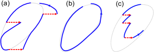
Figure 1: A forced oscillator: (a) strong but sparse forcing, (b) continuous but weak forcing, (c) strong and frequent forcing. Gray dotted curve is the stable limit cycle, blue lines denote trajectories of the system, red dashed lines depict the action of the external pulses.

Therefore, the PRC-based approach is applicable for either weak or sparse stimulation. However, in many realistic situations the stimuli can be strong and frequent. In this case the system pushed away from the limit cycle by one pulse does not return to it by the next pulse arrival (Fig. 1(c)). In such situation, the usual PRC can not account for the effect of the pulse, and a different approach must be used.

In this work we develop a framework for calculation of the oscillator phase response to a series of pulses. The suggested approach is particularly useful when the pulses are frequent or/and strong. In this case the knowledge of the phase at which the pulse arrives does not allow to calculate the phase shift it causes, so that the standard PRC is not applicable. However, we show that the phase shift can still be calculated using the phases at which several last pulses arrived. We call the corresponding function “phase response function” (PRF). We show that the impact of the previous pulses in the PRF falls exponentially with time, which agrees with the experimental evidence that neurons have exponentially decaying memory for past simulations (Vardi2015, ; Goldental2015, ).

The necessity to overcome the limitations of the standard PRC have been recognized previously. As a result, extensions for the PRC have been proposed in (Achuthan2009, ; Oprisan2004, ; Canavier1999, ; Guillamon2009, ; Castej=0000F3n2013, ; Wedgwood2013, ). In particular, in (Achuthan2009, ; Oprisan2004, ; Canavier1999, ), a phenomenological second order PRC was introduced that characterizes the effect that the pulse has on the next cycle beyond the one containing the perturbation. In (Guillamon2009, ; Castej=0000F3n2013, ) the authors introduced the “amplitude response functions” to capture the system’s response depending on the phase and the distance to the cycle. The authors developed numerical algorithm to calculate phase-amplitude response functions which constitutes an extension of the adjoint method for PRCs (Ermentrout1991, ). Somewhat similar but distinct approach was used in (Wedgwood2013, ) where the authors used a transformation to a moving orthonormal coordinate system around the limit cycle.

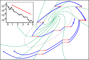
Figure 2: Dynamics of the FitzHugh-Nagumo oscillator receiving pulses at given phases. Gray dotted line shows the limit cycle, green solid dash-dotted lines the isochrons. Two trajectories with different initial conditions are depicted on the phase plane by blue lines, red dashed lines depict the action of the external pulses. Inset: phase difference $\delta\varphi$ versus the phase $\varphi_{k}$. Red line shows the slope $\delta\varphi\sim\mu^{\varphi}$.

In contrast to the previous works, our approach is not limited by the number of significant pulses or the system dimension. The PRF can be computed numerically or measured experimentally for oscillators of arbitrary nature.

The rest of the letter is organized as follows. First, we remind the classical PRC model and introduce the concept of PRF. Then we show how the PRF can be calculated and illustrate it for different oscillatory systems. Finally, we report examples, where the PRF appropriately models dynamics of forced or coupled systems whereas the classical PRC fails.

To start with, we remind the classical PRC-based approximation of an oscillatory system with pulse input. The oscillator is described by the phase $\varphi$ which grows uniformly with $d\varphi/dt=\omega$ except for the time moments $t_{j}$ when the pulses arrive. At these moments, the phase is shifted as

$$\varphi_{j}^{+}=\varphi_{j}^{-}+Z\left(\varphi_{j}^{-}\right),$$ (1)

where $Z(\varphi)$ is the PRC, and $\varphi_{j}^{-}$, $\varphi_{j}^{+}$ are the phases just before and after the pulse arrival at $t_{j}$. The PRC-based approach provides a significant simplification comparing to the study of large realistic systems, since the phase model is one-dimensional, and the effects of the pulses are taken into account discretely at points $t_{j}$.

The standard PRC approximation (1) is valid in the case of weak or sparse pulses. In this work we show that for strong or frequent pulses, the phase shift caused by each pulse at $t_{j}$ can be approximated as

$$\varphi_{j}^{+}=\varphi_{j}^{-}+Z_{n}\left(\varphi_{j-n+1}^{-},\dots,\varphi_{j}^{-}\right).$$ (2)

Here the new function $Z_{n}:\mathbb{R}^{n}\mapsto\mathbb{R}$ is the phase response function (PRF), $\varphi_{j}^{+}$ is the phase just after the pulse at $t_{j},$ and $\varphi_{k}^{-}$ are the phases just before the $k$-th pulse arrival at $t_{k}$. Hence, the phase shift is determined by the phases at which the last $n$ pulses arrived. Effectively, this means the emergence of the dynamical memory: the impact of the current pulse becomes dependent on several previous ones. The number $n$ of the significant pulses depends on how strong and how frequent pulses are. In the case of weak or sparse pulses $n=1$ and the PRF model (2) turns into the PRC model (1).

Thus, the standard PRC is just a particular case of the PRF when the stimulation is weak or sparse. Similarly with PRC, the PRF can be measured numerically or experimentally for an arbitrary oscillator. The direct method to obtain $Z_{n}(\varphi_{1},\varphi_{2},...,\varphi_{n})$ is to stimulate the oscillator by $n$ pulses at the phases $\varphi_{1}$, …,$\varphi_{n}$ and measure the resulting phase shift. We emphasize that the stimulation should be performed at the specified phases, not times. Therefore, the evaluation of the phase after each stimulation is necessary. The detailed description of a possible protocol is given in the Supplemental Material.

Thus, the PRF for a train of any number $n$ of pulses can be directly obtained numerically or experimentally. However, the message of this letter goes beyond this fact – we show that only several recent pulses are significant. The qualitative explanation of this feature is the following. The dynamics of every realistic oscillating system can be split into the phase and the “amplitude” variables, whereas the latter give the distance to the limit cycle. The phase variable is neutrally stable (goldstone mode), while the amplitude dynamics possesses contracting properties in average being in the domain of attraction of the limit cycle. Therefore, the system “forgets” the amplitude variables after a sufficient period of time. In other words, all orbits that are stimulated at the same phases approach each other asymptotically, see blue orbits in Fig. 2.

This idea can be elaborated more precisely for the case of a 2-dimensional system with a stable limit cycle. Following the approach developed in (Guillamon2009, ; Cabre2005, ), such system can be reduced to

$$\dot{\varphi}=\omega,\qquad\dot{\rho}=\lambda\rho$$ (3)

in a neighborhood of the cycle using a nonlinear coordinate transformation. Here $\varphi\in\mathbb{R}(\mod 1)$ is the phase of the system, $\omega=T^{-1}$ is the frequency ($T$ period), $\lambda<0$ is the Floquet exponent, and the variable $\rho$ characterizes the distance to the limit cycle.

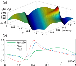
Figure 3: (a) The PRF $Z_{2}(\varphi_{1},\varphi_{2})$ of the Morris-Lecar model. (b) The standard PRC $Z(\varphi)$ (green solid line), the function $F(\varphi)$ (red dash-dot line) and the function $G(\varphi)$ (blue dashed line) of the Morris-Lecar model.

The effect of a short pulse on the oscillator (3) can be given by a map $(\varphi,\rho)\to\left(\varphi^{*},\rho^{*}\right)$ which may be expressed in the form of power series

$$\varphi^{*} = \phi+\varepsilon P(\varphi)+\varepsilon^{2}Q(\varphi)+\varepsilon\rho F(\varphi)+\mathcal{O}(\varepsilon^{3}),$$ (4)

$$\rho^{*} = \rho+\varepsilon G(\varphi)+\mathcal{O}(\varepsilon^{2}),$$ (5)

where $\varepsilon$ is the pulse strength and $P(\varphi)$, $Q(\varphi)$, $F(\varphi)$, $G(\varphi)$ are period-1 functions. Here, we assume that $\rho$ is of the order $\varepsilon$. Note that when the oscillator is on the limit cycle ($\rho=0$), the phase shift caused by the pulse equals to $Z(\varphi)=\varepsilon P(\varphi)+\varepsilon^{2}Q(\varphi)$, which is the standard PRC.

Now consider $n$ pulses arriving at phases $\varphi_{1}<\cdots<\varphi_{n}$ and determine the effect of this pulse train, namely the final phase $\varphi_{n}^{*}$ after the last pulse arrival. If the pulses come sparsely and the oscillator returns to the limit cycle by the arrival of each pulse, the standard PRC may be used. In this case only the last pulse matters, and $\varphi_{n}^{*}=\varphi_{n}+Z(\varphi_{n})$. However, if the pulses are more frequent, the influence of the earlier pulses is not negligible.

To find the final phase in this case, consider the dynamics of the oscillator during the whole pulse train. Each pulse causes the instant shift according to (4)–(5), and between the pulses the system evolves according to (3). This allows to construct a map that transforms the distance $\rho_{k}$ before the $k$-th pulse into the distance $\rho_{k+1}$ before the $(k+1)$-st pulse:

$$\rho_{k+1}=\left(\rho_{k}+\varepsilon G(\varphi_{k})\right)\mu^{\varphi_{k+1}-\varphi_{k}}+\mathcal{O}(\varepsilon^{2}),$$ (6)

where $\mu=e^{\lambda T}$ is the multiplier of the limit cycle. Applying (6) for $k=1,...,n-1$ and substituting the resulting expression for $\rho_{n}$ into (4) gives

$$\varphi_{n}^{*} = \varphi_{n}+\varepsilon P(\varphi_{n})+\varepsilon^{2}Q(\varphi_{n})+\varepsilon\rho_{1}F(\varphi_{n})\mu^{\varphi_{n}-\varphi_{1}}$$ (7)

$$+ \varepsilon^{2}F(\varphi_{n})\sum_{k=1}^{n-1}G(\varphi_{k})\mu^{\varphi_{n}-\varphi_{k}}+O(\varepsilon^{3}).$$

Note that the resulting phase depends on the initial distance $\rho_{1}$. However, the term with $\rho_{1}$ decreases exponentially as the interval between the first and the last pulses increases. The rate of its decay is determined by the multiplier $\mu$, the term decays significantly for $\varphi_{n}-\varphi_{1}\apprge\Theta$, where $\Theta=1/\left|\ln\mu\right|=1/\left|\lambda T\right|$. In this case the influence of the initial distance $\rho_{1}$ is negligible.

This result is illustrated in Fig. 2 where the dynamics of the same oscillator with different initial conditions is illustrated on the phase plane. If the same pulse trains are applied at the same phases $\varphi_{k}$ then the trajectories converge after a short transient.

The above allows us to say that if the pulse train is long enough ($\varphi_{n}-\varphi_{1}\apprge\Theta$), the final phase $\varphi_{n}^{*}$ depends only on the phases $\varphi_{k}$ of the incoming pulses and does not depend on the prehistory $\rho_{1}$. In this case the PRF is given by the phase shift $Z_{n}(\varphi_{1},...,\varphi_{n})=\varphi_{n}^{*}-\varphi_{n}$ that can be approximated as

$$Z_{n}(\varphi_{1},...,\varphi_{n})=Z(\varphi_{n})+\varepsilon^{2}F(\varphi_{n})\sum_{k=1}^{n-1}G(\varphi_{k})\mu^{\varphi_{n}-\varphi_{k}}.$$ (8)

Note that for strong attraction $\mu\to 0$ the PRF transforms to the standard PRC $Z(\varphi_{n}).$ For the finite attraction $\mu>0$, the effect of the past pulses decays exponentially, therefore only those pulses matter whose phases fall into the interval $\varphi_{n}-\varphi_{k}\apprle\Theta$. Hence, the number of the pulses to be taken into account can be estimated as $n\sim f/\left|\lambda T\right|$, where $f$ is the typical frequency at which pulses arrive.

The above analysis not only allowed to estimate the number of significant pulses in the train, but also provides an approximate formula (8) for the PRF. The expression (8) suggests that the system response may be divided into two contributions. The first one is the impact of the current pulse captured by the standard PRC $Z(\varphi_{n})$. The second one represents the “correction” to the PRC due to the impact of the previous pulses. To verify the developed theory we stimulated various oscillators by doublets of pulses at different phases $\varphi_{1}$ and $\varphi_{2}$ and measured the PRF $Z_{2}(\varphi_{1},\varphi_{2})$ directly. Then we checked whether the correction term is given by $Z_{2}(\varphi_{1},\varphi_{2})-Z(\varphi_{1})=\varepsilon^{2}F(\varphi_{2})G(\varphi_{1})\mu^{\varphi_{2}-\varphi_{1}}$ as it should be according to (8). Our tests for several popular oscillatory models – FitzHugh-Nagumo, Morris-Lecar, Hodgkin-Huxley and Van-der-Pol showed remarkable accuracy of this approximation. The details of the protocol and the models are given in the Supplemental Material.

The results of the simulations allowed us to construct the functions $F(\varphi)$ and $G(\varphi)$ for the tested oscillators, see Fig. 3 and Figs. S1-S4. It is remarkable that the function of $n$ variables $Z_{n}(\varphi_{1},...,\varphi_{n})$ can be approximated by functions of a single variable. Moreover, although the approximation (8) is derived for 2D oscillators, it can be practically applicable for higher-dimensional systems, as the example of the Hodgkin-Huxley model shows. A presumable reason for that is the existence of the so-called leading manifold of a stable limit cycle (Shilnikov2001, ) on which the dynamics is governed by (3).

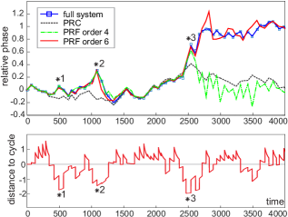
Figure 4: The dynamics of the forced Van-der-Pol oscillator for $\alpha=0.01$, $\varepsilon=1$. The top panel shows the relative phase $\varphi^{\prime}=\varphi-\omega t$, the bottom panel the distance from the limit cycle (positive outside of the cycle and negative inside). On the top panel, the blue solid line with bars shows the dynamics of the full model, black dashed line the PRC approximation, green dash-dot line the approximation by the PRF of the fourth order, red solid line the PRF of the sixth order.

In the following we show examples where the PRF shows essential advantages comparing to PRC. Consider the Van-der-Pol oscillator

$$\ddot{x}-\alpha(1-x^{2})\dot{x}+x=0,$$ (9)

stimulated by pulses that instantly change the variable $x$ to $x+\varepsilon$. For small $\alpha$, the phase $\varphi$ can be introduced geometrically, see (Guckenheimer2013, ; Nekorkin2015, ) and Supplemental Material. Figure 4 illustrates the dynamics of (9) under the action of a pulse train. The pulses are applied at random moments with the inter-pulse intervals distributed homogeneously within the limits $[40,80]$.

One can observe that the PRF approach provides accurate results for the phase dynamics even in the case when the PRC fails. In particular, we compare the results obtained by using the PRF of the sixth order (taking into account 6 last pulses), the fourth order, and the standard PRC. One may see that the standard PRC is sometimes effective, but at certain moments it becomes inaccurate. Particularly, it gives substantial errors at $t\approx 500$ and $t\approx 1100$ (asterisks 1 and 2 on Fig. 4), and becomes absolutely inapplicable at $t\approx 2500$ (asterisk 3) when the error exceeds one. The bottom panel reveals that the PRC fails in the moments when the oscillator goes far from the limit cycle. The same happens with the PRF of the 4-th order. In contrast, the PRF of the 6-th order provides correct results.

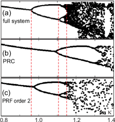
Figure 5: Bifurcation diagram for two coupled Van-der-Pol oscillators and approximations using PRF, $\alpha=2$. (a) Original numeric bifurcation diagram. (b) Diagrams obtained using the approximations with the PRC. (c) Diagram obtained with the PRF of order 2.

As a final demonstration of the PRF advantage, we present a bifurcation diagram in Fig. 5 for the two Van-der-Pol oscillators (9) with pulse coupling. The coupling is organized as follows. When the first oscillator crosses the threshold $x_{1}=0$ from below, the pulse is sent to the second oscillator. The latter is then instantly perturbed so that $x_{2}^{+}=x_{2}^{-}+\kappa x_{2}^{-}$. Similarly, when the second oscillator crosses the threshold, the pulse is sent to the first one.The PRC approximation (Fig. 5(b)) provides qualitatively correct results showing the transition to chaos through a period-doubling cascade. However, the bifurcation points differ significantly from the full system. In contrast, the PRF approach allows to predict these transitions much more accurately (Fig. 5(c)).

To conclude, the concept of PRF provides a novel approach for the modeling of forced or coupled oscillators. It preserves the advantages of the standard PRC-based approach: low dimensionality of the model, computational effectiveness, and the possibility to obtain the PRF for an arbitrary oscillator. At the same time, the PRF remains valid for stronger and more frequent stimulation and thus may capture essentially new dynamical effects. The latter point allows to consider the PRF not only as approximation of full models, but also as a stand-alone model and a test-bed for new phenomena and hypotheses.

Natural application of the PRF is simulation of coupled oscillators (Mirollo1990, ; Bottani1995, ; Herz1995, ; Vreeswijk1996, ; Bressloff1997, ; Izhikevich1999, ; Goel2002, ; Neves2009, ), such as large populations of neurons (Abbot1993, ; Coombes1997, ; Zillmer2007, ; Olmi2010, ; Taylor2011, ), ensembles of chemical (Bar2012, ; Horvath2012, ; Vanag2016, ; Chen2016, ), electronic (Klinshov2014, ; Klinshov2015, ) or optic (Vladimirov2005, ) oscillators. The PRF may be generalized for pulses of different amplitude, which allows to account for inhomogeneous distribution of synaptic weights (Teramae2012, ; Klinshov2014Fukai, ). Coupling delays can also be easily included (Ernst1995, ; Gerstner1996, ; Timme2002a, ; Zeitler2009, ; Klinshov2013, ). Thus, the PRF provides an effective tool for simulation of oscillatory networks which we hope will be demanded in neuroscience and other fields.

Supplementary materials

I The protocol for direct measurement of the PRF

Here we demonstrate how the PRF can be calculated numerically or measured experimentally. Assume we have an oscillator with a stable limit cycle $\gamma$ and we need to obtain the PRF of the order $n$ at a certain point $Z_{n}(\varphi_{1},...,\varphi_{n})$. First we define a specific point $O$ on the cycle with the phase $\varphi_{0}=0$. Then the phase on the limit cycle is well defined as

$$\varphi=\omega(t-t_{0}),$$ (S10)

where $t$ is a current time, $t_{0}$ is the moment of the last passage of point $O$, and $\omega=T^{-1}$, where $T$ is the period of the limit cycle.

On the first step, we set the oscillator to point $O$ at $t=0$, or just wait until it reaches this point. The we apply one pulse at the moment $t_{1}=T\varphi_{1}$. The phase of the oscillator at the pulse arrival equals $\varphi_{1}$. Then we skip a long enough transient assuring the convergence to the limit cycle and measure the phase $\varphi_{c}$ at some moment $t_{c}$. The phase of the unperturbed system would be $\omega t_{c}(\mbox{\,mod\,}1)$, thus we can calculate the phase shift which equals the PRF of the first order

$$Z_{1}(\varphi_{1})=\varphi_{c}-\omega t_{c}\,\,(\mbox{\,mod\,}1).$$ (S11)

On the second step, we reset the oscillator again to point $O$ at $t=0$ and apply two pulses, the first one at the moment $t_{1}=T\varphi_{1}$, and the second one at the moment $t_{2}=T(\varphi_{2}-Z_{1}(\varphi_{1}))$. The phase of the oscillator equals $\varphi_{1}$ at the first pulse arrival, and $\varphi_{2}$ at the second pulse arrival. Thus, measuring the phase $\varphi_{c}$ at moment $t_{c}$ after a long transient, we obtain the PRF of the second order

$$Z_{2}(\varphi_{1},\varphi_{2})=\varphi_{c}-\omega t_{c}(\mod 1).$$ (S12)

Continuing this iterative process one may measure the PRF of any order.

II The impact and the sensitivity functions of various oscillators

To measure the impact and the sensitivity functions of an oscillator, we calculated the second order PRF $Z_{2}(\varphi_{1},\varphi_{2})$ on a grid $(\varphi_{1},\varphi_{2})$. Subtracting the standard PRC allows to find the “correction” $\Delta Z(\varphi_{1},\varphi_{2})=Z_{2}(\varphi_{1},\varphi_{2})-Z(\varphi_{1})$ which should equal according to Eq. (7) of the main text

$$\Delta Z(\varphi_{1},\varphi_{2})=Z_{2}(\varphi_{1},\varphi_{2})-Z(\varphi_{1})=\varepsilon^{2}F(\varphi_{2})G(\varphi_{1})\mu^{\varphi_{2}-\varphi_{1}}.$$ (S13)

A simple and readily verified consequence is that $\Delta Z(\varphi_{1},\varphi_{2}+1)=\mu\Delta Z(\varphi_{1},\varphi_{2})$. We checked that this equality indeed holds with high accuracy, which allows to estimate the value of $\mu$. After that the functions $F(\varphi)$ and $G(\varphi)$ can be estimated as follows. On the first step, we fix $\varphi_{1}$, change $\varphi_{2}$ from zero to one and calculate $F(\varphi_{2})=k\Delta Z(\varphi_{1},\varphi_{2})\mu^{-\varphi_{2}}$. Here $k$ is a normalization coefficient selected so that the maximal absolute value of $F(\varphi)$ equals one. On the second step, we fix $\varphi_{2}$ , change $\varphi_{1}$ from zero to one and use the previously calculated values of $F(\varphi_{2})$ to calculate $G(\varphi_{1})=\varepsilon^{-2}\Delta Z(\varphi_{1},\varphi_{2})\mu^{\varphi_{1}-\varphi_{2}}/F(\varphi_{2})$.

The suggested algorithm has been applied to several oscillatory systems - Moris-Lecar, FitzHugh-Nagumo, Van-der-Pol and Hodgkin-Huxley. Below the details of the models are given and the results are shown. By different colors are plotted the functions $F(\varphi_{2})$ obtained for different $\varphi_{1}$ and the functions $G(\varphi_{1})$ obtained for different $\varphi_{2}$. Note that the difference is small.

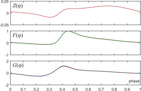
Figure S6: The results for the Morris-Lecar model.

The Morris-Lecar model (Morris1981, ) is given by the system

$$C_{M}\frac{dV}{dt} = I-g_{L}\left(V-V_{L}\right)-g_{K}m\left(V-V_{K}\right)-g_{Ca}\frac{1+\tanh\frac{V-V_{1}}{V_{2}}}{2}\left(V-V_{Ca}\right),$$ (S14)

$$\frac{dm}{dt} = \phi\cosh\frac{V-V_{3}}{2V_{4}}\left(\frac{1+\tanh\frac{V-V_{3}}{V_{4}}}{2}-m\right).$$ (S15)

with $I=100$, $C_{M}=50$, $g_{Ca}=4$, $g_{K}=8$, $g_{L}=2$, $V_{Ca}=120$, $V_{K}=-80$, $V_{L}=-60$, $\phi=0.04$, $V_{1}=-1.2$, $V_{2}=18$, $V_{3}=10$, $V_{4}=17$. The pulse instantly changes $V$ by the value $\Delta V=2$. The results are given in Fig. 3 of the main text and Fig. S1.

Figure S7: The results for the FitzHugh-Nagumo model.

The FitzHugh-Nagumo model (FitzHugh1961, ; Nagumo1962, ) is given by the system

$$\frac{dv}{dt} = I+v-\frac{v^{3}}{3}-u,$$ (S16)

$$\frac{du}{dt} = a\left(v+b-cu\right).$$ (S17)

with $I=1$, $a=0.8$, $b=0.7$, $c=0.8$. The pulse instantly changes $v$ by the value $\Delta v=0.2$. The results are given in Fig. S2.

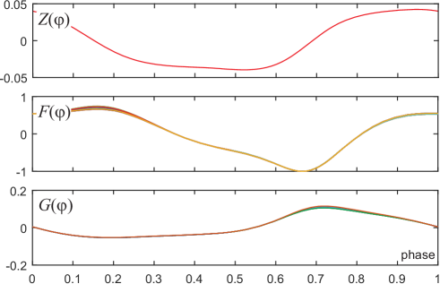
Figure S8: The results for the Van der Pol model.

The Van-der-Pol oscillator (VdP1926, ) is given by the equation

$$\frac{d^{2}x}{dx^{2}}-\alpha\left(1-x^{2}\right)\frac{dx}{dt}+x=0$$ (S18)

with $\alpha=0.2$. The pulse changes $x$ by the value $\Delta x=0.5$. The results are given in Fig. S3.

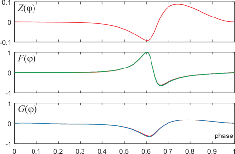
Figure S9: The results for the Hodgkin-Huxley model.

The Hodgkin-Huxley model (HH1952, ) is given by the system

$$C_{M}\frac{dV}{dt} = I-g_{K}n^{4}\left(V-V_{K}\right)-g_{Na}m^{3}h\left(V-V_{Na}\right)-g_{l}\left(V-V_{L}\right),$$ (S19)

$$\frac{dn}{dt} = \frac{0.01V+0.55}{1-\exp\left(-0.1V-5.5\right)}\left(1-n\right)-0.125\exp\left(\frac{-V-65}{80}\right)n,$$ (S20)

$$\frac{dm}{dt} = \frac{0.1V+4}{1-\exp\left(-0.1V-4\right)}\left(1-m\right)-4\exp\left(\frac{-V-65}{18}\right)m,$$ (S21)

$$\frac{dh}{dt} = 0.07\exp\left(\frac{-V-65}{20}\right)\left(1-h\right)-\frac{1}{1+\exp\left(-0.1V-3.5\right)}h$$ (S22)

with $C_{M}=1$, $I=10$, $g_{Na}=120$, $g_{K}=36$, $g_{L}=0.3$, $V_{Na}=50$, $V_{K}=-77$, $V_{l}=-54.5$. The pulse changes $V$ by $\Delta V=3$. The results are given in Fig. S4.

III The analysis of the Van-der-Pol oscillator

First, we rewrite (9) of the main text as

$$\frac{dx}{dt} = y,$$ (S23)

$$\frac{dy}{dt} = \alpha y(1-x^{2})-x.$$ (S24)

Then, we introduce the polar coordinates $\varphi$ and $R$ so that $x=R\cos 2\pi\varphi$ and $y=-R\sin 2\pi\varphi$. Substituting this into (2),(3) results in

$$\dot{R}\cos 2\pi\varphi-2\pi\dot{\phi}R\sin 2\pi\varphi = -R\sin 2\pi\varphi,$$ (S25)

$$-\dot{R}\sin 2\pi\varphi-2\pi\dot{\varphi}R\cos 2\pi\varphi = -\alpha R\sin 2\pi\varphi\left(1-R^{2}\cos^{2}2\pi\varphi\right)-R\cos 2\pi\varphi,$$ (S26)

where the dot means is the derivative over time. From (4), (5) one can express $\dot{R}$ and $\dot{\varphi}$ as

$$\dot{R} = \alpha R\sin^{2}2\pi\phi\left(1-R^{2}\cos 2\pi\varphi\right),$$ (S27)

$$\dot{\phi} = \frac{1}{2\pi}\left(1+\alpha\sin 2\pi\varphi\cos 2\pi\varphi\left(1-R^{2}\cos^{2}2\pi\varphi\right)\right).$$ (S28)

Note that $\dot{\phi}\approx 1$ for $\alpha\ll 1$, and the right parts of (6), (7) may be averaged (Guckenheimer2013, ; Nekorkin2015, ) leading to

$$\dot{R} = \frac{1}{8}\alpha R\left(4-R^{2}\right),$$ (S29)

$$\dot{\varphi} = \frac{1}{2\pi}.$$ (S30)

Easy to see that the variable change $\rho=1-4/R^{2}$ transforms (8), (9) into

$$\dot{\varphi} = \omega,$$ (S31)

$$\dot{\rho} = \lambda\rho$$ (S32)

with $\omega=1/(2\pi)$, $\lambda=-\alpha$. Thus, for $\alpha\ll 1$ the variable $\varphi$ is the oscillator’s phase.

References

- (1) C. Morris, and H. Lecar. Biophysic. J. 35, 193 (1981)
- (2) R. FitzHugh. Biophysical J. 1, 445 (1961)
- (3) J. Nagumo, S. Arimoto, and S. Yoshizawa. Proc IRE 50, 2061 (1962)
- (4) B. Van der Pol. The London, Edinburgh, and Dublin Philosophical Magazine and Journal of Science 2, 978 (1926)
- (5) A.L. Hodgkin, and A.F. Huxley. J. Physiol 117, 500 (1952)
- (6) J. Guckenheimer, and P.J. Holmes. Nonlinear oscillations, dynamical systems, and bifurcations of vector fields (Springer-Verlag New York, 1983).
- (7) V.I. Nekorkin. Introduction to nonlinear oscillations (Wiley-VCH, 2015).