Deep Sketch Hashing: Fast Free-hand Sketch-Based Image Retrieval

Abstract

Free-hand sketch-based image retrieval (SBIR) is a specific cross-view retrieval task, in which queries are abstract and ambiguous sketches while the retrieval database is formed with natural images. Work in this area mainly focuses on extracting representative and shared features for sketches and natural images. However, these can neither cope well with the geometric distortion between sketches and images nor be feasible for large-scale SBIR due to the heavy continuous-valued distance computation. In this paper, we speed up SBIR by introducing a novel binary coding method, named Deep Sketch Hashing (DSH), where a semi-heterogeneous deep architecture is proposed and incorporated into an end-to-end binary coding framework. Specifically, three convolutional neural networks are utilized to encode free-hand sketches, natural images and, especially, the auxiliary sketch-tokens which are adopted as bridges to mitigate the sketch-image geometric distortion. The learned DSH codes can effectively capture the cross-view similarities as well as the intrinsic semantic correlations between different categories. To the best of our knowledge, DSH is the first hashing work specifically designed for category-level SBIR with an end-to-end deep architecture. The proposed DSH is comprehensively evaluated on two large-scale datasets of TU-Berlin Extension and Sketchy, and the experiments consistently show DSH’s superior SBIR accuracies over several state-of-the-art methods, while achieving significantly reduced retrieval time and memory footprint.

1 Introduction

Content-based image retrieval (CBIR) or text-based retrieval (TBR) has played a major role in practical computer vision applications. In some scenarios, however, if example queries are not available or it is difficult to describe them with keywords, what should we do? To address such a problem, sketch-based image retrieval (SBIR) [13, 19, 46, 69, 42, 47, 3, 12, 27, 21, 57, 6, 7, 20, 62, 43, 49] has been recently developed and is becoming popular in information retrieval area (as shown in Fig. 1). Compared to traditional retrieval approaches, using a sketch query can more efficiently and precisely express the shape, pose and fine-grained details of the search target, which is intuitive to humans and far more convenient than describing it with a “hundred” words in text.

Figure 1: An illustration of the SBIR concept in this paper. Given a free-hand query, we aim to retrieve relevant natural images in the same category as the query from the gallery.

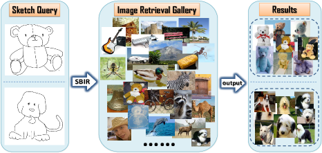
However, SBIR is challenging since humans draw free-hand sketches without any reference but only focus on the salient object structures. As such, the shapes and scales in sketches are usually distorted compared to natural images. To deal with this problem, some studies have attempted to bridge the domain gap between sketches and natural images for SBIR. These methods can be roughly divided into two groups: hand-crafted methods and cross-domain deep learning-based methods.

Hand-crafted SBIR first generates approximate sketches by extracting edge or contour maps from the natural images. After that, hand-crafted features (e.g., SIFT [39], HOG [8], gradient field HOG [18, 19], histogram of edge local orientations (HELO) [48, 46] and Learned KeyShapes (LKS) [47]) are extracted for both sketches and edgemaps of natural images, which are then fed into “Bag-of-Words” (BoW) methods to generate the representations for SBIR. The major limitation of hand-crafted methods is that the domain gap between sketches and natural images cannot be well remedied, as it is difficult to match edge maps to non-aligned sketches with large variations and ambiguity.

To further improve the above domain shift issue, convolutional neural networks (CNNs) [24] have been recently used to learn domain-transformable features from sketches and images with end-to-end frameworks [49, 43, 62]. Being able to better handle the domain gap, deep methods typically achieve higher performance than hand-crafted ones for both category-level [13, 19, 46, 69, 42, 47, 12] and fine-grained [49, 62, 27] SBIR tasks.

Although achieving progress, current deep SBIR methods are still facing severe challenges. In particular, these methods tend to perform well in the situation that each of the gallery images contains only a single object with a simple contour shape on a clean background (e.g., “Moon”, “Eiffel-tower” and “Pyramid” in the shape-based Flickr15K dataset [19]). In practice, however, objects in gallery images may appear from various viewpoints with relatively complex backgrounds (e.g., a rhinoceros in bushes). In such a case, current methods fail to handle the significant geometric distortions between free-hand sketches and natural images, and result in unsatisfactory performance.

Moreover, less study has been devoted to the searching efficiency of SBIR. Most SBIR techniques are based on applying nearest neighbor (NN) searches with computational complexity $\mathcal{O}(Nd)$ on continuous-valued features (hand-crafted or deeply learned). Such methods become inappropriate for large-scale SBIR tasks in certain realistic scenarios (e.g., on wearable or mobile devices). Therefore, being able to conduct a fast SBIR on a substantial number of images with limited computational and memory resources is crucial for practical applications.

To address the above issues, in this paper, we introduce a novel Deep Sketch Hashing (DSH) framework for the fast free-hand SBIR, which incorporates the learning of binary codes and deep hash functions into a unified framework. Specifically, DSH speeds up SBIR by embedding sketches and natural images into two sets of compact binary codes, aiming at not only preserving their pairwise semantic similarities, but also leveraging the intrinsic category correlations. Unlike previous methods with Siamese [43, 57] or triplet CNNs [49, 62] only utilizing images and sketches, we propose a novel semi-heterogeneous deep architecture including three CNNs, where a unique middle-level network fed with “sketch-tokens” is developed to effectively diminish the aforementioned geometric distortion between free-hand sketches and natural images. The contributions of this work mainly include:

• To the best of our knowledge, DSH is the first hashing work specifically designed for category-level SBIR, where both binary codes and deep hash functions are learned in a joint end-to-end framework. DSH aims to generate binary codes which can successfully capture the cross-view relationship (between images and sketches) as well as the intrinsic semantic correlations between different categories. To this end, an efficient alternating optimization scheme is applied to produce the high-quality hash codes.

• A novel semi-heterogeneous deep architecture is developed in DSH as the hash function, where natural images, free-hand sketches and the auxiliary sketch-tokens are fed into three CNNs (as shown in Fig. 3). Particularly, natural images and their corresponding sketch-tokens are fed into a heterogeneous late-fusion net, while the CNNs for sketches and sketch-tokens share the same weights during training. As such, the architecture in DSH can better remedy the domain gap between images and sketches compared to previous SBIR deep nets.

• The experiments consistently illustrate superior performance of DSH compared to the state-of-the-art methods, while achieving significant reduction on both retrieval time and memory load.

Related Work

Hashing techniques [16, 33, 58, 38, 34, 17, 70, 35, 14, 66, 36, 44, 37, 51, 25, 32] have recently been successfully applied to encode high-dimensional features into compact similarity-preserving binary codes, which enables extremely fast similarity search by the use of Hamming distances. Inspired by this, some recent SBIR works [1, 15, 40, 52, 54, 56] have incorporated existing hashing methods for efficient retrieval. For instance, LSH [16] and ITQ [17] are adopted to sketch-based image [1] and 3D model [15] retrieval tasks, respectively. In fact, among various hashing methods, cross-modality hashing [30, 64, 68, 26, 31, 2, 53, 71, 67, 10, 23, 5, 4], which learns binary codes by preserving the correlations between heterogeneous representations from different modalities, are more related to SBIR problems. However, all of the above hashing techniques are not specifically designed for SBIR and neglect the intrinsic relationship between free-hand sketches and natural images, resulting in unsatisfactory performance.

In the next section, we will introduce the detailed architecture of our deep hash nets in DSH, then elaborate on our hashing objective function.

2 Deep Sketch Hashing

To help better understand this section, we first introduce some notation. Let $\mathcal{O}_{1}=\{\mathbf{I}_{i},\mathbf{Z}_{i}\}^{n_{1}}_{i=1}$, where $\mathbf{I}_{i}$ is a natural image and $\mathbf{Z}_{i}$ is its corresponding sketch-token computed from $\mathbf{I}_{i}$; $\mathcal{O}_{2}=\{\mathbf{S}_{j}\}^{n_{2}}_{j=1}$ be the set of free-hand sketches $\mathbf{S}_{j}$; and $n_{1}$ and $n_{2}$ indicate the numbers of the samples in $\mathcal{O}_{1}$ and $\mathcal{O}_{2}$, respectively. Additionally, define the label matrix $\mathbf{Y}^{I}=\{\mathbf{y}^{I}_{i}\}^{n_{1}}_{i=1}\in\mathbb{R}^{C\times n_{1}}$, where $y_{ci}^{I}=1$ if $\{\mathbf{I}_{i},\mathbf{Z}_{i}\}$ belongs to class $c$ and $0$ otherwise; $\mathbf{Y}^{S}=\{\mathbf{y}^{S}_{j}\}_{j=1}^{n_{2}}\in\mathbb{R}^{C\times n_{2}}$ for sketches is defined in the same way. We aim to learn two sets of $m$-bit binary codes $\mathbf{\mathbf{B}}^{I}=\{\mathbf{b}^{I}_{i}\}^{n_{1}}_{i=1}\in\{-1,1\}^{m\times n_{1}}$ and $\mathbf{B}^{S}=\{\mathbf{b}^{S}_{j}\}^{n_{2}}_{j=1}\in\{-1,1\}^{m\times n_{2}}$ for $\mathcal{O}_{1}$ and $\mathcal{O}_{2}$, respectively.

2.1 Semi-heterogeneous Deep Architecture

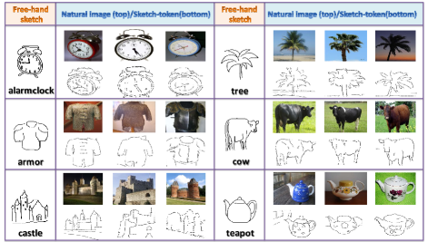
As previously stated, SBIR is a very challenging task due to large geometric distortion between sketches and images. Inspired by [29, 47], in this work, we propose to adopt an auxiliary image representation as a bridge to mitigate the geometric distortion between sketch and natural images. In particular, a set of edge structures are detected from natural images, called “sketch-tokens”, using supervised middle-level information in the form of hand-drawn sketches. In practice, given an image we will get an initial sketch-token, where each pixel is assigned a score for the likeliness of it being a contour point. We then use 60% of the maximum score (same as [47]) to threshold each pixel and obtain the final sketch-tokens as shown in Fig. 2.

Sketch-tokens have two advantages: (1) they reflect only essential edges of natural images without detailed texture information; (2) unlike ordinary edgemaps (e.g., Canny), they have very similar stroke patterns and appearance to free-hand sketches. Next, we will show how to design the DSH architecture with the help of sketch-tokens.

Figure 2: Illustration of our DSH inputs: free-hand sketches, natural images and corresponding sketch-tokens. Sketch-tokens have similar stroke patterns and appearance to free-hand sketches.

We propose a novel semi-heterogeneous deep architecture, where three CNNs are developed as hash functions to encode free-hand sketches, natural images and auxiliary sketch-tokens into binary codes. As shown in Fig. 3, the DSH framework includes the following two parts:

1) Cross-weight Late-fusion Net: A heterogeneous net with two parallel CNNs is developed, termed C1-Net (Bottom) and C2-Net (Middle). Particularly, C1-Net (bottom) is slightly modified from AlexNet [24] containing 5 convolutional (conv) layers and 2 fully connected (fc) layers for natural image inputs, while C2-Net is configured with 4 convolutional layers and 2 fully connected layers for corresponding sketch-token inputs. The detailed parameters are listed in Table 1. Inspired by the recent multimodal deep framework [45], we connected the pooling3, fc_a, fc_b of both C1-Net (Bottom) and C2-Net (Middle) with cross-weights. In this way, we exploit high-level interactions between two nets to maximize the mutual information across both modalities, while the information from each individual net is also preserved. Finally, similar to [30, 10], we late-fuse the C1-Net (Bottom) and C2-Net (Middle) into a unified binary coding layer hash_C1 so that the learned codes can fully benefit from both natural images and their corresponding sketch-tokens.

Table 1: The detailed configuration of the proposed DSH.

Net	Layer	Kernel Size	Stride	Pad	Output
C1-Net (Natural Image)	input	-	-	-	3$\times$227$\times$227
	conv1	11$\times$11	4	0	96$\times$55$\times$55
	pooling1	3$\times$3	2	0	96$\times$27$\times$27
	conv2	5$\times$5	1	2	256$\times$27$\times$27
	pooling2	3$\times$3	2	0	256$\times$13$\times$13
	conv3	3$\times$3	1	1	384$\times$13$\times$13
	conv4	3$\times$3	1	1	384$\times$13$\times$13
	conv5	3$\times$3	1	1	384$\times$13$\times$13
	pooling3	3$\times$3	2	1	256$\times$7$\times$7
	fc_a	7$\times$7	1	0	4096$\times$1$\times$1
	fc_b	1$\times$1	1	0	1024$\times$1$\times$1
	hash_C1	1$\times$1	1	0	$m$ $\times$1$\times$1
C2-Net (Free-hand sketch/ Sketch- tokens )	input	-	-	-	1$\times$200$\times$200
	conv1	14$\times$14	3	0	64$\times$63$\times$63
	pooling1	3$\times$3	2	0	64$\times$31$\times$31
	conv2_1	3$\times$3	1	1	128$\times$31$\times$31
	conv2_2	3$\times$3	1	1	128$\times$31$\times$31
	pooling2	3$\times$3	2	0	128$\times$15$\times$15
	conv3_1	3$\times$3	1	1	256$\times$15$\times$15
	conv3_2	3$\times$3	1	1	256$\times$15$\times$15
	pooling3	3$\times$3	2	0	256$\times$7$\times$7
	fc_a	7$\times$7	1	0	4096$\times$1$\times$1
	fc_b	1$\times$1	1	0	1024$\times$1$\times$1
	hash_C2	1$\times$1	1	0	$m$ $\times$1$\times$1

2) Shared-weight Sketch Net: For free-hand sketch inputs, we develop the C2-Net (Top) with configurations shown in Table 1. Specifically, considering the similar characteristics and implicit correlations existing between sketch-tokens and free-hand sketches as mentioned above, we design a Siamese architecture for C2-Net (Middle) and C2-Net (Top) to share the same deep weights in conv and fc layers during the optimization (see in Fig. 3). As such, the hash codes of free-hand sketches learned via the shared-weight net (from hash_C2) will mitigate the geometric difference between images and sketches during SBIR.

Figure 3: The illustration of the main idea of the proposed DSH. Specifically, we integrate a convolutional neural network and discrete binary code learning into a unified end-to-end framework which can be effectively optimized in an alternating manner.

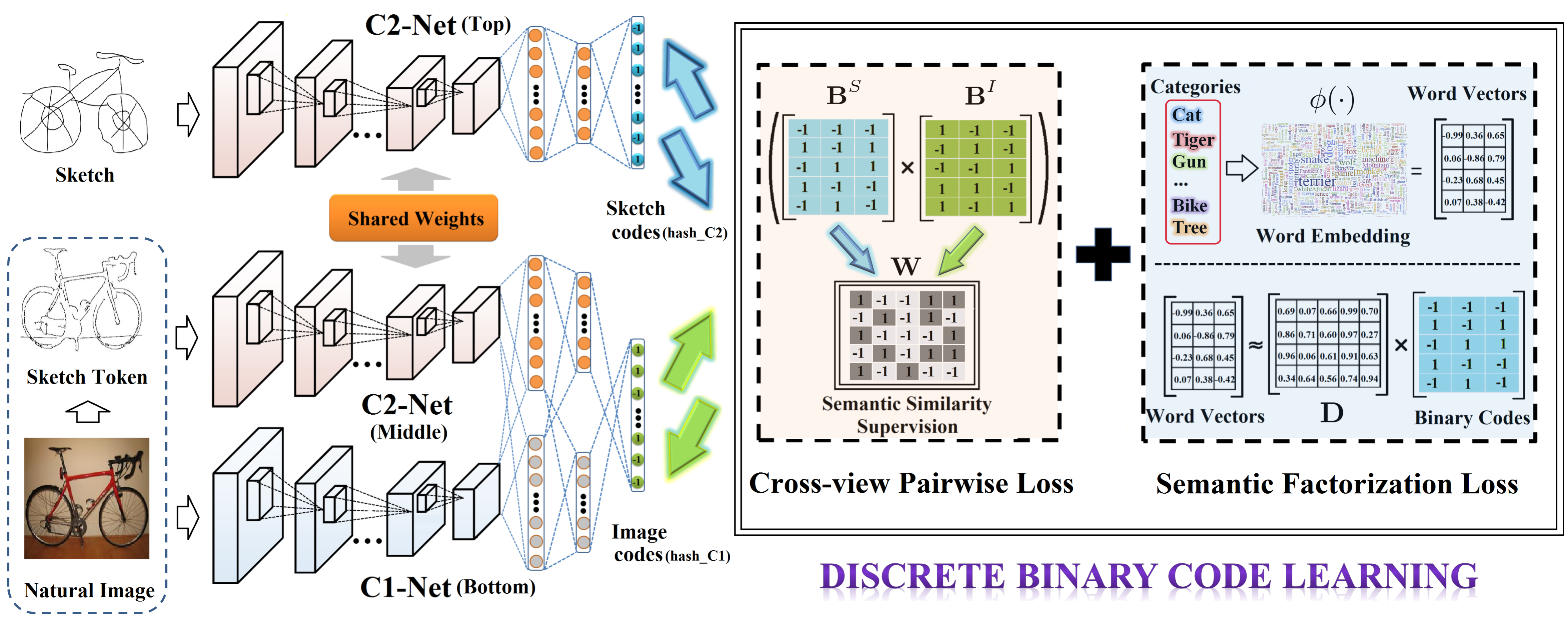
Deep Hash Functions: Denote by $\Theta_{1}$ the deep weights in C1-Net (Bottom) and $\Theta_{2}$ the shared weights in C2-Net (Middle) and C2-Net (Top). For natural images and their sketch-tokens, we form the deep hash function $\mathbf{B}^{I}=\operatorname{sign}(\mathbf{F}_{1}(\mathcal{O}_{1};\Theta_{1},\Theta_{2}))$ from the cross-weight late-fusion net of C1-Net (Bottom) and C2-Net (Middle). Similarly, the shared-weight sketch net (i.e., C2-Net (Top)) is regarded as the hash function $\mathbf{B}^{S}=\operatorname{sign}(\mathbf{F}_{2}(\mathcal{O}_{2};\Theta_{2}))$ for free-hand sketches. In this way, hash codes learned from the above deep hash functions can lead to more reasonable SBIR, especially when a significant sketch-image distortion exists. Next, we will introduce the DSH objective of joint learning of binary codes and hash functions.

2.2 Objective Formulation of DSH

1) Cross-view Pairwise Loss: We first define the cross-view similarity matrix of $\mathcal{O}_{1}$ and $\mathcal{O}_{2}$ as $\mathbf{W}\in\mathbb{R}^{n_{1}\times n_{2}}$, where the element of $\mathbf{W}_{ij}$ denotes the cross-view similarity between $\{\mathbf{\mathbf{I}}_{i},\mathbf{\mathbf{Z}}_{i}\}$ and $\mathbf{S}_{j}$. The inner product of learned $\mathbf{B}^{I}$ and $\mathbf{B}^{S}$ should sufficiently approximate the similarity matrix $\mathbf{W}$. Thus, we consider the following problem:

$$\underset{\mathbf{B}^{I},\mathbf{B}^{S}}{\min}\mathcal{J}_{1}:=||\mathbf{W}\odot m-{\mathbf{B}^{I}}^{\top}\mathbf{B}^{S}||^{2},$$ (1)

$$\mathrm{s.t.}\ \mathbf{B}^{I}\in\{-1,+1\}^{m\times n_{1}},\ \mathbf{B}^{S}\in\{-1,+1\}^{m\times n_{2}},$$

where $||\cdot||$ is the Frobenius norm and $\odot$ is the element-wise product. The cross-view similarity matrix $\mathbf{W}$ can be defined by semantic label information as $\mathbf{W}_{ij}=1$ if $\mathbf{y}^{I}_{i}=\mathbf{y}^{S}_{j}$ and $-1$ otherwise. By Eq.(1), the binary codes of natural images and sketches from the same category will be pulled as close as possible and pushed far away otherwise.

2) Semantic Factorization Loss: Beyond the cross-view similarity, we also consider preserving the intra-set semantic relationships for both the image set $\mathcal{O}_{1}$ and the sketch set $\mathcal{O}_{2}$. However, the given 0/1 label matrices $\mathbf{Y}^{I}$ and $\mathbf{Y}^{S}$ can only provide binary measurements (i.e., the samples belong to the same category or not), which causes all different categories to have equivalent distance (e.g., “cheetah” will be as different from “tiger” as from “dolphin”). Thus, directly using such discrete label information will implicitly make all categories independent and discards the latent correlation of high-level semantics.

Inspired by the recent development of word embeddings [41], in this paper, we overcome the above drawback by utilizing the NLP word-vector toolbox to map the independent labels into the high-level semantic space. As such, the intrinsic semantic correlation among different labels can be quantitatively measured and captured (e.g., the semantic embedding of “cheetah” will be closer to “tiger” but further from “dolphin”). As semantic embeddings intentionally guide the learning of high-quality binary codes, we optimize the following semantic factorization problem

$$\underset{\mathbf{B}^{I},\mathbf{B}^{S}}{\min}\mathcal{J}_{2}:=||\phi(\mathbf{Y}^{I})-\mathbf{D}\mathbf{B}^{I}||^{2}+||\phi(\mathbf{Y}^{S})-\mathbf{D}\mathbf{B}^{S}||^{2},$$ (2)

$$\mathrm{s.t.}\ \mathbf{B}^{I}\in\{-1,+1\}^{m\times n_{1}},\ \mathbf{B}^{S}\in\{-1,+1\}^{m\times n_{2}},$$

where $\phi(\cdot)$ is the word embedding model, $\phi(\mathbf{Y}^{I})\in\mathbb{R}^{d\times n_{1}}$ and $\phi(\mathbf{Y}^{S})\in\mathbb{R}^{d\times n_{2}}$, $d=1000$ is the dimension of word embedding. $\mathbf{D}\in\mathbb{R}^{d\times m}$ is the shared basis of the semantic factorization for both views. Note that the shared basis we used helps to preserve the latent semantic correlations which also benefits cross-view code learning in SBIR.

Final Objective Function: Unlike previous hashing methods using continuous-relaxation during code learning, we keep the binary constraints in the DSH optimization. By recalling Eq.(1) and Eq.(2), we obtain our final objective function:

$$\underset{\mathbf{B}^{I},\mathbf{B}^{S},\mathbf{D}^{I},\mathbf{D}^{S},\Theta_{1},\Theta_{2}}{\min}\mathcal{J}:=||\mathbf{W}\odot m-{\mathbf{B}^{I}}^{\top}\mathbf{B}^{S}||^{2}$$ (3)

$$+\lambda(||\phi(\mathbf{Y}^{I})-\mathbf{D}\mathbf{B}^{I}||^{2}+||\phi(\mathbf{Y}^{S})-\mathbf{D}\mathbf{B}^{S}||^{2})$$

$$+\gamma(||\mathbf{F}_{1}(\mathcal{O}_{1};\Theta_{1},\Theta_{2})-\mathbf{B}^{I}||^{2}+||\mathbf{F}_{2}(\mathcal{O}_{2};\Theta_{2})-\mathbf{B}^{S}||^{2}),$$

$$\mathrm{s.t.}\ \mathbf{B}^{I}\in\{-1,+1\}^{m\times n_{1}},\ \mathbf{B}^{S}\in\{-1,+1\}^{m\times n_{2}}.$$

Here, $\lambda>0$ and $\gamma>0$ are the balance parameters. The last two regularization terms aim to minimize the quantization loss between binary codes $\mathbf{B}^{I}$, $\mathbf{B}^{S}$ and deep hash functions $\mathbf{F}_{1}(\mathcal{O}_{1};\Theta_{1},\Theta_{2})$, $\mathbf{F}_{2}(\mathcal{O}_{2};\Theta_{2})$. Similar regularization terms are also used in [50, 36] for effective hash code learning. Next, we will elaborate on how to optimize problem (3).

3 Optimization

It is clear that problem (3) is non-convex and non-smooth, which is in general an NP-hard problem due to the binary constraints. To address this, we propose an alternating optimization based algorithm, which sequentially updates $\mathbf{D}$, $\mathbf{B^{I}}$, $\mathbf{B^{S}}$ and deep hash functions $\mathbf{F}_{1}/\mathbf{F}_{2}$ in an iterative fashion. In practice, we first pre-train C1-Net (Bottom) and C2-Net (Top) as classification nets using natural images and sketches with corresponding semantic labels. After that, pre-trained models will be applied in our semi-heterogeneous deep model as in Fig. 3 and then optimized with the following alternating steps.

$\mathbf{D}$ Update Step.

By fixing all variables except for $\mathbf{D}$, Eq.(3) shrinks to a classic quadratic regression problem

$$\underset{\mathbf{D}}{\min}\ ||\phi(\mathbf{Y}^{I})-\mathbf{D}\mathbf{B}^{I}||^{2}+||\phi(\mathbf{Y}^{S})-\mathbf{D}\mathbf{B}^{S}||^{2},$$ (4)

which can be solved analytically as

$$\mathbf{D}=(\phi(\mathbf{Y}^{I}){\mathbf{B}^{I}}^{\top}+\phi(\mathbf{Y}^{S}){\mathbf{B}^{S}}^{\top})(\mathbf{B}^{I}{\mathbf{B}^{I}}^{\top}+\mathbf{B}^{S}{\mathbf{B}^{S}}^{\top})^{-1}.$$ (5)

$\mathbf{B}^{I}$ Update Step.

By fixing all other variables, we optimize $\mathbf{B}^{I}$ by the following equation

$$\underset{\mathbf{B}^{I}}{\min}\ ||\mathbf{W}\odot m-{\mathbf{B}^{I}}^{\top}\mathbf{B}^{S}||^{2}+\lambda||\phi(\mathbf{Y}^{I})-\mathbf{D}\mathbf{B}^{I}||^{2}$$ (6)

$$+\gamma||\mathbf{F}_{1}(\mathcal{O}_{1};\Theta_{1},\Theta_{2})-\mathbf{B}^{I}||^{2},$$

$$\mathrm{s.t.}\ \mathbf{B}^{I}\in\{-1,+1\}^{m\times n_{1}}.$$

We further rewrite (6) as

$$\underset{\mathbf{B}^{I}}{\min}\ ||{\mathbf{B}^{I}}^{\top}\mathbf{B}^{S}||^{2}+\lambda||{\mathbf{B}^{I}}^{\top}{\mathbf{D}}^{\top}||^{2}-2\operatorname{trace}({\mathbf{B}^{I}}^{\top}\mathbf{R}),$$ (7)

$$\mathrm{s.t.}\ \mathbf{B}^{I}\in\{-1,+1\}^{m\times n_{1}},$$

where $\mathbf{R}=\mathbf{B}^{S}(\mathbf{W}^{\top}\odot m)+\lambda{\mathbf{D}}^{\top}\phi(\mathbf{Y}^{I})+\gamma\mathbf{F}_{1}(\mathcal{O}_{1};\Theta_{1},\Theta_{2})$ and $||\mathbf{B}^{I}||^{2}=mn_{1}$.

Algorithm 1     Deep Sketch Hashing (DSH)

1:Set of pairs of natural images and corresponding sketch-tokens $\mathcal{O}_{1}=\{\mathbf{I}_{i}\,\mathbf{Z}_{i}\}_{i=1}^{n_{1}}$; Free-hand sketch set $\mathcal{O}_{2}=\{\mathbf{S}_{J}\}_{J=1}^{n_{2}}$; The label information $\{\mathbf{y}^{I}_{i}\}_{i=1}^{n_{1}}$ and $\{\mathbf{y}^{S}_{j}\}_{j=1}^{n_{2}}$; Total epochs $T$ of deep optimization.

2:Deep hash functions $\mathbf{F}_{1}(\mathcal{O}_{1};\Theta_{1},\Theta_{2})$ and $\mathbf{F}_{2}(\mathcal{O}_{2};\Theta_{2})$.

3:Randomly initialize $\{\mathbf{b}^{I}_{i}\}^{n_{1}}_{i=1}\in\{-1,+1\}^{m\times n_{1}}$ and $\{\mathbf{b}^{S}_{j}\}^{n_{2}}_{j=1}\in\{-1,+1\}^{m\times n2}$ for the entire training set; construct cross-view similarity matrix $\mathbf{W}\in\mathbb{R}^{n_{1}\times n_{2}}$.

4:For $t=1,\ldots,T$ epoch do

5:   Update $\mathbf{D}$ according to Eq.(5);

6:   Update $\mathbf{B}^{I}$ and $\mathbf{B}^{S}$ according to Eq.(10);

7:   Update the deep parameters {$\Theta_{1}$,$\Theta_{2}$} by $t^{th}$ epoch data;

8:End

It is challenging to directly optimize $\mathbf{B}^{I}$ with discrete constraints. Inspired by the discrete cyclic coordinate descent (DCC) [51], we learn each row of $\mathbf{B}^{I}$ by fixing all other $m-1$ rows, i.e., each time we only optimize one single bit of all $n_{1}$ samples. We denote $\mathbf{\widehat{b}}^{I}_{k}$, $\mathbf{\widehat{b}}^{S}_{k}$, $\mathbf{\widehat{r}}_{k}$ and $\mbox{$\mathbf{\widehat{d}}_{k}$}^{\top}$ as the $k^{th}$ rows of $\mathbf{B}^{I}$, $\mathbf{B}^{S}$, $\mathbf{R}$ and $\mathbf{D}^{\top}$ respectively, $k=1,\ldots,m$. For convenience, we also have

$$\small\vspace{-1ex}\left\{\begin{array}[]{lll}\mathbf{\widehat{B}}^{I}_{\neg k}&=&[\mbox{$\mathbf{\widehat{b}}^{I}_{1}$}^{\top},\ldots,\mbox{$\mathbf{\widehat{b}}^{I}_{k-1}$}^{\top},\mbox{$\mathbf{\widehat{b}}^{I}_{k+1}$}^{\top},\ldots,\mbox{$\mathbf{\widehat{b}}^{I}_{m}$}^{\top}]^{\top},\\ \mathbf{\widehat{B}}^{S}_{\neg k}&=&[\mbox{$\mathbf{\widehat{b}}^{S}_{1}$}^{\top},\ldots,\mbox{$\mathbf{\widehat{b}}^{S}_{k-1}$}^{\top},\mbox{$\mathbf{\widehat{b}}^{S}_{k+1}$}^{\top},\ldots,\mbox{$\mathbf{\widehat{b}}^{S}_{m}$}^{\top}]^{\top},\\ \mathbf{\widehat{D}}_{\neg k}&=&[\mbox{$\mathbf{\widehat{d}}_{1}$},\ldots,\mbox{$\mathbf{\widehat{d}}_{k-1}$},\mbox{$\mathbf{\widehat{d}}_{k+1}$},\ldots,\mbox{$\mathbf{\widehat{d}}_{m}$}].\end{array}\right.$$ (8)

It is not difficult to show Eq.(7) can be rewritten w.r.t. $\mathbf{\widehat{b}}^{I}_{k}$ as

$$\underset{\widehat{\mathbf{b}}^{I}_{k}}{\min}\ \widehat{\mathbf{b}}^{I}_{k}(\mbox{$\mathbf{\widehat{B}}^{I}_{\neg k}$}^{\top}\widehat{\mathbf{B}}^{S}_{\neg k}\mbox{$\widehat{\mathbf{b}}^{S}_{k}$}^{\top}+\lambda\mbox{$\mathbf{\widehat{B}}^{I}_{\neg k}$}^{\top}\mbox{$\mathbf{\widehat{D}}_{\neg k}$}^{\top}\mathbf{\widehat{d}}_{k}-{\mathbf{\widehat{r}}_{k}}^{\top}),$$ (9)

$$\mathrm{s.t.}\ \mathbf{\widehat{b}}^{I}\in\{-1,+1\}^{1\times n_{1}}.$$

Thus, the closed-form solution for the $k^{th}$ row of $\mathbf{B}^{I}$ can be obtained by

$$\mathbf{\widehat{b}}^{I}_{k}=\operatorname{sign}({\mathbf{\widehat{r}}_{k}}-\mbox{$\widehat{\mathbf{b}}^{S}_{k}$}\mbox{$\widehat{\mathbf{B}}^{S}_{\neg k}$}^{\top}\mbox{$\mathbf{\widehat{B}}^{I}_{\neg k}$}-\lambda\mbox{$\mathbf{\widehat{d}}_{k}$}^{\top}\mbox{$\mathbf{\widehat{D}}_{\neg k}$}\mbox{$\mathbf{\widehat{B}}^{I}_{\neg k}$}).$$ (10)

In this way, the binary codes $\mathbf{B}^{I}$ can be optimized bit by bit and finally reach a stationary point.

$\mathbf{B}^{S}$ Update Step.

By fixing all other variables, we learn hash code $\mathbf{B}^{S}$ with a similar formulation to Eq.(10).

$\Theta_{1}$ and $\Theta_{2}$ Update Step.

Once $\mathbf{B}^{I}$ and $\mathbf{B}^{S}$ are obtained, we update parameters $\Theta_{1}$ and $\Theta_{2}$ of C1-Net and C2-Net according to the following Euclidean loss:

$$\underset{\Theta_{1},\Theta_{2}}{\min}\ \mathcal{L}:=||\mathbf{F}_{1}(\mathcal{O}_{1};\Theta_{1},\Theta_{2})-\mathbf{B}^{I}||^{2}+||\mathbf{F}_{2}(\mathcal{O}_{2};\Theta_{2})-\mathbf{B}^{S}||^{2}.\vspace{1ex}$$ (11)

By first computing the partial gradients $\frac{\partial\mathcal{L}}{\partial\mathbf{F}_{1}(\Theta_{1},\Theta_{2})}$ and $\frac{\partial\mathcal{L}}{\partial\mathbf{F}_{2}(\Theta_{2})}$, we can obtian $\frac{\partial\mathcal{L}}{\partial(\Theta_{1},\Theta_{2})}$ by the chain rule. We then use the standard mini-batch back-propagation (BP) scheme to simultaneously update $\Theta_{1}$ and $\Theta_{2}$ for our entire deep architecture. In practice, the above procedure can be easily achieved by deep learning toolboxes (e.g., Caffe [22]).

Figure 4: The illustration of DSH alternating optimization scheme.

Table 2: Comparison with previous SBIR methods (MAP, Precision@200, Retrieval time ($\mathrm{s}$)/query and Memory load ($\mathrm{MB}$)) on both datasets. Apart from DSH producing binary codes, the continuous-value feature representations are utilized by all other methods.

Methods	Dimension	TU-Berlin Extension				Sketchy
		MAP	Precision @200	Retrieval time per query ($\mathrm{s}$)	Memory load($\mathrm{MB}$) (204,489 gallery images)	MAP	Precision @200	Retrieval time per query ($\mathrm{s}$)	Memory load($\mathrm{MB}$) (73,002 gallery images)
HOG [8]	1296	0.091	0.120	1.43	$2.02\times 10^{3}$	0.115	0.159	0.53	$7.22\times 10^{2}$
GF-HOG [18]	3500	0.119	0.148	4.13	$5.46\times 10^{3}$	0.157	0.177	1.41	$1.95\times 10^{3}$
SHELO [46]	1296	0.123	0.155	1.44	$2.02\times 10^{3}$	0.161	0.182	0.50	$7.22\times 10^{2}$
LKS [47]	1350	0.157	0.204	1.51	$2.11\times 10^{3}$	0.190	0.230	0.56	$7.52\times 10^{2}$
Siamese CNN [43]	64	0.322	0.447	7.70$\times 10^{-2}$	99.8	0.481	0.612	2.76$\times 10^{-2}$	35.4
SaN [63]	512	0.154	0.225	0.53	$7.98\times 10^{2}$	0.208	0.292	0.21	$2.85\times 10^{2}$
GN Triplet∗ [49]	1024	0.187	0.301	1.02	$1.60\times 10^{3}$	0.529	0.716	0.41	$5.70\times 10^{2}$
3D shape∗ [57]	64	0.054	0.072	7.53$\times 10^{-2}$	99.8 $\mathrm{MB}$	0.084	0.079	2.64 $\times 10^{-2}$	35.6
Siamese-AlexNet	4096	0.367	0.476	5.35	$6.39\times 10^{3}$	0.518	0.690	1.68	$2.28\times 10^{3}$
Triplet-AlexNet	4096	0.448	0.552	5.35	$6.39\times 10^{3}$	0.573	0.761	1.68 $\mathrm{s}$	$2.28\times 10^{3}$
DSH (Proposed)	32 (bits)	0.358	0.486	5.57$\times 10^{-4}$	0.78	0.653	0.797	2.55$\times 10^{-4}$	0.28
	64 (bits)	0.521	0.655	7.03$\times 10^{-4}$	1.56	0.711	0.858	2.82$\times 10^{-4}$	0.56
	128 (bits)	0.570	0.694	1.05$\times 10^{-3}$	3.12	0.783	0.866	3.53$\times 10^{-4}$	1.11

’*’ denotes we directly use the public models provided by the original papers without any fine-tuning on TU-Berlin Extension or Sketchy datasets.

As shown in Fig. 4, we iteratively update $\mathbf{D}\rightarrow\mathbf{B}^{I}\rightarrow\mathbf{B}^{S}\rightarrow\{\Theta_{1},\Theta_{2}\}$ in each epoch. As such, DSH can be finally optimized within $T$ epochs in total, where $T=10\sim 15$. Notice that the overall objective is lower-bounded, thus the convergence of (3) is always guaranteed by coordinate descent used in our optimization. The overall DSH is summarized in Algorithm 1.

Once the DSH model is trained, given a sketch query $\mathbf{S}_{q}$, we can compute its binary code $\mathbf{b}^{S_{q}}=\operatorname{sign}(\mathbf{F}_{2}(\mathbf{S}_{q};\Theta_{2}))$ with C2-Net (Top). For the retrieval database, the unified hash code of each image and sketch-token pair $\{\mathbf{I},\mathbf{Z}\}$ is computed as $\mathbf{b}^{I}=\operatorname{sign}(\mathbf{F}_{1}(\mathbf{I},\mathbf{Z};\Theta_{1},\Theta_{2}))$ with C1-Net (Bottom) and C2-Net (Middle).

4 Experiments

In this section, we conduct extensive evaluations of DSH on the two largest SBIR datasets: TU-Berlin Extension and Sketchy. Our method is implemented using Caffe with dual K80 GPUs for training our deep models and MATLAB 2015b on an i7 4790K CPU for binary coding.

4.1 Datasets and Protocols

Datasets: TU-Berlin [11] Extension contains 250 object categories with 80 free-hand sketches for each category. We also use 204,489 extended natural images associated to TU-Berlin provided by [65] as our natural image retrieval gallery. Sketchy [49] is a newly released dataset originally for fine-grained SBIR, in which 75,471 hand-drawn sketches of 12,500 objects (images) from 125 categories are included. To better fit the task of large-scale SBIR in our paper, we collect another 60,502 natural images (an average of 484 images/category) ourselves from ImageNet [9] to form a new retrieval gallery with 73,002 images in total. Similar to previous hashing evaluations, we randomly select 10 and 50 sketches from each category as the query sets for TU-Berlin and Sketchy respectively, and the remaining sketches and gallery images are used for training.

Table 3: Category-level SBIR using different cross-modality methods. For non-deep methods, 4096-d AlexNet fc7 image features and 512-d SaN fc7 sketch features are used. For deep methods, raw natural images and sketches are used.

Method		TU-Berlin Extension						Sketchy
		MAP			Precision@200			MAP			Precision@200
		32 bits	64 bits	128 bits	32 bits	64 bits	128 bits	32 bits	64 bits	128 bits	32 bits	64 bits	128 bits
Cross-Modality Hashing Methods (binary codes)	CMFH [10]	0.149	0.202	0.180	0.168	0.282	0.241	0.320	0.490	0.190	0.489	0.657	0.286
	CMSSH [2]	0.121	0.183	0.175	0.143	0.261	0.233	0.206	0.211	0.211	0.371	0.376	0.375
	SCM-Seq [64]	0.211	0.276	0.332	0.298	0.372	0.454	0.306	0.417	0.671	0.442	0.529	0.758
	SCM-Orth [64]	0.217	0.301	0.263	0.312	0.420	0.470	0.346	0.536	0.616	0.467	0.650	0.776
	CVH [26]	0.214	0.294	0.318	0.305	0.411	0.449	0.325	0.525	0.624	0.459	0.641	0.773
	SePH [30]	0.198	0.270	0.282	0.307	0.380	0.398	0.534	0.607	0.640	0.694	0.741	0.768
	DCMH [23]	0.274	0.382	0.425	0.332	0.467	0.540	0.560	0.622	0.656	0.730	0.771	0.784
Proposed	DSH	0.358	0.521	0.570	0.486	0.655	0.694	0.653	0.711	0.783	0.797	0.858	0.866
Cross-View Feature Learning Methods (continuous-value vectors)	CCA [55]	0.276	0.366	0.365	0.333	0.482	0.536	0.361	0.555	0.705	0.379	0.610	0.775
	XQDA [28]	0.191	0.197	0.201	0.263	0.278	0.278	0.460	0.557	0.550	0.607	0.715	0.727
	PLSR [59]	0.141 (4096-d)			0.215 (4096-d)			0.462 (4096-d)			0.623 (4096-d)
	CVFL [60]	0.289 (4096-d)			0.407 (4096-d)			0.675 (4096-d)			0.803 (4096-d)

PLSR and CVFL are both based on reconstructing partial data to approximate full data, so the dimensions are fixed to 4096-d.

Figure 5: Precision-recall curves and HD2 precision on both TU-Berlin Extension and Sketchy datasets.

Compared Methods and Implementation Details: We first compare the proposed DSH with several previous SBIR methods, including hand-crafted HOG [8], GF-HOG [18], SEHLO [46], LSK [47]; and deep learning based Siamese CNN [43], Sketch-a-Net (SaN) [63], GN Triplet [49], 3D shape [57]. For HOG, GF-HOG, SEHLO, Siamese CNN and 3D shape, we need first to compute Canny edgemaps from natural images and then extract the features. In detail, we compute GF-HOG via a BoW scheme with a codebook size 3500; for HOG, SEHLO and LSK, we exactly follow the best settings used in [47]. Due to lack of stroke order information in the Sketchy dataset, we only use a single deep channel SaN in our experiments as in [62]. We fine-tune Siamese CNN and SaN on TU-Berlin and Sketchy datasets, while the public models of GN Triplet and 3D shape are only allowed for direct feature extraction without any re-training. Additionally, we add Siamese-AlexNet (with contrastive loss) and Triplet-AlexNet (with triplet ranking loss) as the baselines, both of which are constructed and trained by ourselves on two datasets. Particularly, the semantic pairwise/triplet supervision for our Siamese/Triplet-AlexNet are constructed the same as [43]/[61] respectively.

Moreover, DSH is also compared with state-of-the-art cross-modality hashing techniques: Collective Matrix Factorization Hashing (CMFH) [10], Cross-Modal Semi-Supervised Hashing (CMSSH) [2], Cross-View Hashing (CVH) [26], Semantic Correlation Maximization (SCM-Seq and SCM-Orth) [64], Semantics-Preserving Hashing (SePH) [30] and Deep Cross-Modality Hashing (DCMH) [23]. Note that since DCMH is a deep hashing method originally for image-text retrieval, in our experiments, we modify it into a Siamese net by replacing the text embedding channel with an identical parallel image channel. In addition, another four cross-view feature embedding methods: CCA [55], PLSR [59], XQDA [28] and CVFL [60] are used for comparison. Except for DCMH, each image and sketch in both datasets are represented by 4096-d AlexNet [24] fc7 and 512-d SaN fc7 deep features, respectively. Since these hashing and feature embedding methods need pairwise data with corresponding labels as inputs, in our experiments, we further construct these deep features (extracted from TU-Berlin Extension/Sketchy datasets) into 100,000 sample pairs (with 800/400 pairs per category) to train all of the above cross-modality methods.

For the proposed DSH, we train our deep model using SGD on Caffe with an initial learning rate $\alpha$$=$0.001, momentum$=$0.9 and batch size 64. We decrease $\alpha\rightarrow 0.3\alpha$ every epoch and terminate the optimization after 15 epochs. For both datasets, our balance parameters are set to $\lambda$=$0.01$ and $\gamma$=$10^{-5}$ via cross validation on training sets.

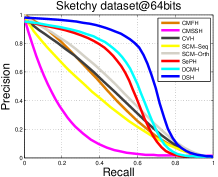
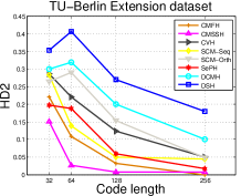
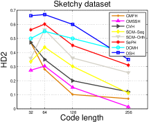
In the test phase, we report the mean average precision (MAP) and precision at top-rank 200 (precision@200) to evaluate the category-level SBIR. For all hashing methods, we also evaluate the precision of Hamming distance with radius 2 (HD2) and the precision-recall curves. Additionally, we report the retrieval time per query ($\mathrm{s}$) from image galleries and memory loads (MB) for compared methods.

Figure 6: The visualization of our SBIR: eight example query sketches with their top-20 retrieval results on Sketchy dataset by using 128-bit DSH codes. Red boxes indicates false positives. (More examples can be seen in our supplementary documents.)

4.2 Results and Discussions

DSH vs. SBIR Baselines: In Table 2, we demonstrate the comparison of MAP and precision@200 over all SBIR methods on two datasets. Generally, deep learning-based methods can achieve much better performance than hand-crafted methods and the results on Sketchy are higher than those on TU-Berlin Extension since the data in Sketchy is relatively simpler with fewer categories. Our 128-bit DSH leads to superior results with 0.138/0.142 and 0.210/0.105 improvements (MAP/precision@200) over the best-performing comparison methods on the two datasets, respectively. This is because the semi-heterogeneous deep architecture of DSH is specifically designed for category-level SBIR by effectively introducing the auxiliary sketch-tokens to mitigate the geometric distortion between free-hand sketches and natural images. The other deep methods: Siamese CNN, GN Triplet and 3D shape only incorporate images and sketches as training data with a simple multi-channel deep structure. Among the compared methods, we notice 3D shape produces worse SBIR performance than previous papers [57, 62] reported. In [62], the images from the retrieval gallery all contain well-aligned objects with perfect background removal, thus the edgemaps computed from such images can well represent the objects and have almost identical stroke patterns with free-hand sketches, which guarantees a good SBIR performance. However, in our tasks, all images in the retrieval gallery are realistic with relatively complex backgrounds and there is still a big dissimilarity between the computed edgemaps and sketches. Therefore, 3D shape features extracted from our edgemaps become ineffective. Similar problems also exist in SaN, HOG and SHELO. In addition, the retrieval time and memory load are listed in Table 2. Our DSH can achieve significantly faster speed with much lower memory load compared to conventional SBIR methods during retrieval.

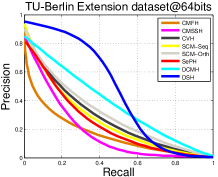
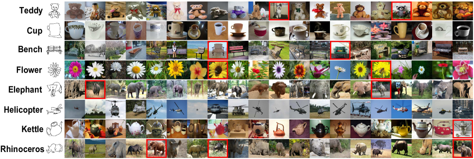
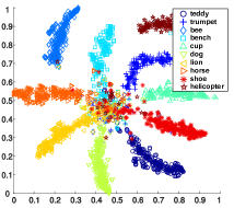
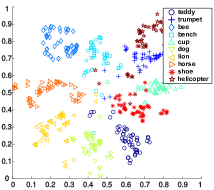
DSH vs. Cross-modality Hashing: We also compare our DSH with cross-modality hashing/feature learning methods in Table 3. As mentioned before, we use the learned deep features as the inputs for non-deep methods to achieve a fair comparison with our DSH. In particular, SCM-Orth and SePH always lead to high accuracies among compared non-deep hashing methods on both datasets. With its deep end-to-end structure, DCMH can achieve better results than non-deep hashing methods, while CMFH and CMSSH produce the weakest results due to un(semi-)supervised learning mechanisms. For cross-view feature learning schemes, CCA and CVFL achieve superior performance on TU-Berlin Extension and Sketchy datasets, respectively. Our DSH can consistently outperform all other methods in Table 3. The superior performance of DSH is also demonstrated in 64-bit precision-recall curves and HD2 curves along different code lengths (shown in Fig. 5) by comparing the Area Under the Curve (AUC). Besides, we illustrate $t$-SNE visualization in Fig. 7 where the analogous DSH distributions of the test sketches and image gallery intuitively reflect the effectiveness of DSH codes. Lastly, some query examples with top-20 SBIR retrieval results are shown in Fig. 6.

(a) Image retrieval gallery	(b) Test sketch queries

Figure 7: $t$-SNE visualization of 32-bit DSH codes of 10 representative categories in the Sketchy dataset. After DSH, natural images (a) and test sketch queries (b) from the same categories are almost scattered into the same clusters. Meanwhile, semantically similar categories are distributed closely and otherwise far away.

DSH Component Analysis: We have evaluated the effectiveness of different components of DSH in Table 4. Specifically, we construct a heterogeneous deep net by only using C2-Net (Top) and C1-Net (Bottom) channels with the same binary coding scheme. It produces around $0.073$ and $0.101$ MAP decreases by only using images and sketches on the respective datasets, which sufficiently proves the importance of sketch-tokens in order to mitigate the geometric distortion. We also observe that only using either the cross-view pairwise loss term or the semantic factorization loss term will result in worse performance than applying the full model, since the cross-view similarities and the intrinsic semantic correlations captured in DSH can complement each other and simultaneously benefit the final MAPs.

Table 4: Effectiveness (MAP 128 bits) of different components.

Method	TU-Berlin Extension	Sketchy
C2-Net (Top) + C1-Net (Bottom) only	0.497	0.682
C2-Net (Top) + C2-Net (Middle) only	0.379	0.507
Using Cross-view Pairwise Loss only	0.522	0.715
Using Semantic Factorization Loss only	0.485	0.667
Our proposed full DSH model	0.570	0.783

5 Conclusion

In this paper, we proposed a novel deep hashing framework, named deep sketch hashing (DSH), for fast sketch-based image retrieval (SBIR). Particularly, a semi-heterogeneous deep architecture was designed to encode free-hand sketches and natural images, together with the auxiliary sketch-tokens which can effectively mitigate the geometric distortion between the two modalities. To train DSH, binary codes and deep hash functions were jointly optimized in an alternating manner. Extensive experiments validated the superiority of DSH over the state-of-the-art methods in terms of retrieval accuracy and time/storage complexity.

References

- [1] K. Bozas and E. Izquierdo. Large scale sketch based image retrieval using patch hashing. In International Symposium on Visual Computing, 2012.
- [2] M. M. Bronstein, A. M. Bronstein, F. Michel, and N. Paragios. Data fusion through cross-modality metric learning using similarity-sensitive hashing. In CVPR, 2010.
- [3] X. Cao, H. Zhang, S. Liu, X. Guo, and L. Lin. Sym-fish: A symmetry-aware flip invariant sketch histogram shape descriptor. In CVPR, 2013.
- [4] Y. Cao, M. Long, and J. Wang. Correlation hashing network for efficient cross-modal retrieval. arXiv preprint arXiv:1602.06697, 2016.
- [5] Y. Cao, M. Long, J. Wang, Q. Yang, and P. S. Yu. Deep visual-semantic hashing for cross-modal retrieval. In KDD, 2016.
- [6] Y. Cao, C. Wang, L. Zhang, and L. Zhang. Edgel index for large-scale sketch-based image search. In CVPR, 2011.
- [7] Y. Cao, H. Wang, C. Wang, Z. Li, L. Zhang, and L. Zhang. Mindfinder: interactive sketch-based image search on millions of images. In ACM MM, 2010.
- [8] N. Dalal and B. Triggs. Histograms of oriented gradients for human detection. In CVPR, 2005.
- [9] J. Deng, W. Dong, R. Socher, L.-J. Li, K. Li, and L. Fei-Fei. Imagenet: A large-scale hierarchical image database. In CVPR, pages 248–255. IEEE, 2009.
- [10] G. Ding, Y. Guo, and J. Zhou. Collective matrix factorization hashing for multimodal data. In CVPR, 2014.
- [11] M. Eitz, J. Hays, and M. Alexa. How do humans sketch objects? ACM Trans. Graph., 31(4):44–1, 2012.
- [12] M. Eitz, K. Hildebrand, T. Boubekeur, and M. Alexa. An evaluation of descriptors for large-scale image retrieval from sketched feature lines. Computers & Graphics, 34(5):482–498, 2010.
- [13] M. Eitz, K. Hildebrand, T. Boubekeur, and M. Alexa. Sketch-based image retrieval: Benchmark and bag-of-features descriptors. IEEE Transactions on Visualization and Computer Graphics, 17(11):1624–1636, 2011.
- [14] V. Erin Liong, J. Lu, G. Wang, P. Moulin, and J. Zhou. Deep hashing for compact binary codes learning. In CVPR, 2015.
- [15] T. Furuya and R. Ohbuchi. Hashing cross-modal manifold for scalable sketch-based 3d model retrieval. In International Conference on 3D Vision, 2014.
- [16] A. Gionis, P. Indyk, R. Motwani, et al. Similarity search in high dimensions via hashing. In VLDB, volume 99, pages 518–529, 1999.
- [17] Y. Gong, S. Lazebnik, A. Gordo, and F. Perronnin. Iterative quantization: A procrustean approach to learning binary codes for large-scale image retrieval. T-PAMI, 35(12):2916–2929, 2013.
- [18] R. Hu, M. Barnard, and J. Collomosse. Gradient field descriptor for sketch based retrieval and localization. In ICIP, 2010.
- [19] R. Hu and J. Collomosse. A performance evaluation of gradient field hog descriptor for sketch based image retrieval. Computer Vision and Image Understanding, 117(7):790–806, 2013.
- [20] R. Hu, T. Wang, and J. Collomosse. A bag-of-regions approach to sketch-based image retrieval. In ICIP, 2011.
- [21] S. James, M. J. Fonseca, and J. Collomosse. Reenact: Sketch based choreographic design from archival dance footage. In ICMR, 2014.
- [22] Y. Jia, E. Shelhamer, J. Donahue, S. Karayev, J. Long, R. Girshick, S. Guadarrama, and T. Darrell. Caffe: Convolutional architecture for fast feature embedding. In ACM MM, 2014.
- [23] Q.-Y. Jiang and W.-J. Li. Deep cross-modal hashing. arXiv preprint arXiv:1602.02255, 2016.
- [24] A. Krizhevsky, I. Sutskever, and G. E. Hinton. Imagenet classification with deep convolutional neural networks. In NIPS, 2012.
- [25] B. Kulis and K. Grauman. Kernelized locality-sensitive hashing for scalable image search. In CVPR, 2009.
- [26] S. Kumar and R. Udupa. Learning hash functions for cross-view similarity search. In IJCAI, 2011.
- [27] K. Li, K. Pang, Y.-Z. Song, T. Hospedales, H. Zhang, and Y. Hu. Fine-grained sketch-based image retrieval: The role of part-aware attributes. In WACV, 2016.
- [28] S. Liao, Y. Hu, X. Zhu, and S. Z. Li. Person re-identification by local maximal occurrence representation and metric learning. In CVPR, 2015.
- [29] J. J. Lim, C. L. Zitnick, and P. Dollár. Sketch tokens: A learned mid-level representation for contour and object detection. In CVPR, 2013.
- [30] Z. Lin, G. Ding, M. Hu, and J. Wang. Semantics-preserving hashing for cross-view retrieval. In CVPR, 2015.
- [31] L. Liu, Z. Lin, L. Shao, F. Shen, G. Ding, and J. Han. Sequential discrete hashing for scalable cross-modality similarity retrieval. TIP, 26(1):107–118, 2017.
- [32] L. Liu and L. Shao. Sequential compact code learning for unsupervised image hashing. TNNLS, 27(12):2526–2536, 2016.
- [33] L. Liu, M. Yu, and L. Shao. Multiview alignment hashing for efficient image search. TIP, 24(3):956–966, 2015.
- [34] L. Liu, M. Yu, and L. Shao. Projection bank: From high-dimensional data to medium-length binary codes. In ICCV, 2015.
- [35] L. Liu, M. Yu, and L. Shao. Latent struture preserving hashing. IJCV, 2016.
- [36] W. Liu, C. Mu, S. Kumar, and S.-F. Chang. Discrete graph hashing. In NIPS, 2014.
- [37] W. Liu, J. Wang, R. Ji, Y.-G. Jiang, and S.-F. Chang. Supervised hashing with kernels. In CVPR, 2012.
- [38] W. Liu, J. Wang, S. Kumar, and S.-F. Chang. Hashing with graphs. In ICML, 2011.
- [39] D. G. Lowe. Object recognition from local scale-invariant features. In CVPR, 1999.
- [40] Y. Matsui, K. Aizawa, and Y. Jing. Sketch2manga: Sketch-based manga retrieval. In ICIP, 2014.
- [41] T. Mikolov, I. Sutskever, K. Chen, G. S. Corrado, and J. Dean. Distributed representations of words and phrases and their compositionality. In NIPS, 2013.
- [42] S. Parui and A. Mittal. Similarity-invariant sketch-based image retrieval in large databases. In ECCV, 2014.
- [43] Y. Qi, Y.-Z. Song, H. Zhang, and J. Liu. Sketch-based image retrieval via siamese convolutional neural network. In ICIP, 2016.
- [44] M. Raginsky and S. Lazebnik. Locality-sensitive binary codes from shift-invariant kernels. In NIPS, 2009.
- [45] S. Rastegar, M. Soleymani, H. R. Rabiee, and S. Mohsen Shojaee. Mdl-cw: A multimodal deep learning framework with cross weights. In CVPR, 2016.
- [46] J. M. Saavedra. Sketch based image retrieval using a soft computation of the histogram of edge local orientations (s-helo). In ICIP, 2014.
- [47] J. M. Saavedra, J. M. Barrios, and S. Orand. Sketch based image retrieval using learned keyshapes (lks). 2015.
- [48] J. M. Saavedra and B. Bustos. An improved histogram of edge local orientations for sketch-based image retrieval. In Joint Pattern Recognition Symposium, 2010.
- [49] P. Sangkloy, N. Burnell, C. Ham, and J. Hays. The sketchy database: learning to retrieve badly drawn bunnies. ACM Transactions on Graphic, 35(4):119, 2016.
- [50] F. Shen, W. Liu, S. Zhang, Y. Yang, and H. T. Shen. Learning binary codes for maximum inner product search. In ICCV, 2015.
- [51] F. Shen, C. Shen, W. Liu, and H. Tao Shen. Supervised discrete hashing. In CVPR, 2015.
- [52] B. Siddiquie, B. White, A. Sharma, and L. S. Davis. Multi-modal image retrieval for complex queries using small codes. In ACM MM.
- [53] J. Song, Y. Yang, Y. Yang, Z. Huang, and H. T. Shen. Inter-media hashing for large-scale retrieval from heterogeneous data sources. In ACM SIGMOD, 2013.
- [54] X. Sun, C. Wang, C. Xu, and L. Zhang. Indexing billions of images for sketch-based retrieval. In ACM MM, pages 233–242, 2013.
- [55] B. Thompson. Canonical correlation analysis. Encyclopedia of statistics in behavioral science, 2005.
- [56] K.-Y. Tseng, Y.-L. Lin, Y.-H. Chen, and W. H. Hsu. Sketch-based image retrieval on mobile devices using compact hash bits. In ACM MM, pages 913–916, 2012.
- [57] F. Wang, L. Kang, and Y. Li. Sketch-based 3d shape retrieval using convolutional neural networks. In CVPR, 2015.
- [58] Y. Weiss, A. Torralba, and R. Fergus. Spectral hashing. In NIPS, 2008.
- [59] H. Wold. Partial least squares. Encyclopedia of statistical sciences, 1985.
- [60] W. Xie, Y. Peng, and J. Xiao. Cross-view feature learning for scalable social image analysis. In AAAI, 2014.
- [61] T. Yao, F. Long, T. Mei, and Y. Rui. Deep semantic-preserving and ranking-based hashing for image retrieval. In IJCAI, 2016.
- [62] Q. Yu, F. Liu, Y.-Z. Song, T. Xiang, T. M. Hospedales, and C. C. Loy. Sketch me that shoe. In CVPR, 2016.
- [63] Q. Yu, Y. Yang, Y.-Z. Song, T. Xiang, and T. Hospedales. Sketch-a-net that beats humans. In BMVC, 2015.
- [64] D. Zhang and W.-J. Li. Large-scale supervised multimodal hashing with semantic correlation maximization. In AAAI, 2014.
- [65] H. Zhang, S. Liu, C. Zhang, W. Ren, R. Wang, and X. Cao. Sketchnet: sketch classification with web images. In CVPR, 2016.
- [66] Z. Zhang, Y. Chen, and V. Saligrama. Efficient training of very deep neural networks for supervised hashing. In CVPR, 2016.
- [67] Y. Zhen and D.-Y. Yeung. Co-regularized hashing for multimodal data. In NIPS, 2012.
- [68] J. Zhou, G. Ding, and Y. Guo. Latent semantic sparse hashing for cross-modal similarity search. In ACM SIGIR, 2014.
- [69] R. Zhou, L. Chen, and L. Zhang. Sketch-based image retrieval on a large scale database. In ACM MM, pages 973–976, 2012.
- [70] H. Zhu, M. Long, J. Wang, and Y. Cao. Deep hashing network for efficient similarity retrieval. In AAAI, 2016.
- [71] X. Zhu, Z. Huang, H. T. Shen, and X. Zhao. Linear cross-modal hashing for efficient multimedia search. In ACM MM, 2013.