Minimum Perimeter-Sum Partitions in the Plane

Abstract

Let $P$ be a set of $n$ points in the plane. We consider the problem of partitioning $P$ into two subsets $P_{1}$ and $P_{2}$ such that the sum of the perimeters of $\mbox{\sc ch}(P_{1})$ and $\mbox{\sc ch}(P_{2})$ is minimized, where $\mbox{\sc ch}(P_{i})$ denotes the convex hull of $P_{i}$. The problem was first studied by Mitchell and Wynters in 1991 who gave an $O(n^{2})$ time algorithm. Despite considerable progress on related problems, no subquadratic time algorithm for this problem was found so far. We present an exact algorithm solving the problem in $O(n\log^{2}n)$ time and a $(1+\varepsilon)$-approximation algorithm running in $O(n+1/\varepsilon^{2}\cdot\log^{2}(1/\varepsilon))$ time.

1 Introduction

The clustering problem is to partition a given data set into clusters (that is, subsets) according to some measure of optimality. We are interested in clustering problems where the data set is a set $P$ of points in Euclidean space. Most of these clustering problems fall into one of two categories: problems where the maximum cost of a cluster is given and the goal is to find a clustering consisting of a minimum number of clusters, and problems where the number of clusters is given and the goal is to find a clustering of minimum total cost. In this paper we consider a basic problem of the latter type, where we wish to find a bipartition $(P_{1},P_{2})$ of a planar point set $P$. Bipartition problems are not only interesting in their own right, but also because bipartition algorithms can form the basis of hierarchical clustering methods.

There are many possible variants of the bipartition problem on planar point sets, which differ in how the cost of a clustering is defined. A variant that received a lot of attention is the 2-center problem [9, 11, 12, 15, 21], where the cost of a partition $(P_{1},P_{2})$ of the given point set $P$ is defined as the maximum of the radii of the smallest enclosing disks of $P_{1}$ and $P_{2}$. Other cost functions that have been studied include the maximum diameter of the two point sets [5] and the sum of the diameters [14]; see also the survey by Agarwal and Sharir [3] for some more variants.

A natural class of cost functions considers the size of the convex hulls $\mbox{\sc ch}(P_{1})$ and $\mbox{\sc ch}(P_{2})$ of the two subsets, where the size of $\mbox{\sc ch}(P_{i})$ can either be defined as the area of $\mbox{\sc ch}(P_{i})$ or as the perimeter $\mathrm{per}(P_{i})$ of $\mbox{\sc ch}(P_{i})$. (The perimeter of $\mbox{\sc ch}(P_{i})$ is the length of the boundary $\partial\hskip 1.42262pt{\mbox{\sc ch}(P_{i})}$.) This class of cost functions was already studied in 1991 by Mitchell and Wynters [17]. They studied four problem variants: minimize the sum of the perimeters, the maximum of the perimeters, the sum of the areas, or the maximum of the areas. In three of the four variants the convex hulls $\mbox{\sc ch}(P_{1})$ and $\mbox{\sc ch}(P_{2})$ in an optimal solution may intersect [17, full version]—only in the minimum perimeter-sum problem the optimal bipartition is guaranteed to be a so-called line partition, that is, a solution with disjoint convex hulls. For each of the four variants they gave an $O(n^{3})$ algorithm that uses $O(n)$ storage and that computes an optimal line partition; for all except the minimum area-maximum problem they also gave an $O(n^{2})$ algorithm that uses $O(n^{2})$ storage. Note that (only) for the minimum perimeter-sum problem the computed solution is an optimal bipartition. Around the same time, the minimum-perimeter sum problem was studied for partitions into $k$ subsets for $k>2$; for this variant Capoyleas et al. [8] presented an algorithm with running time $O(n^{6k})$. Arkin et al. [4] studied the same problem and gave a similar algorithm. Very recently, Abrahamsen et al. [1] gave an algorithm for that problem running in time $O(n^{28})$, even when $k$ is part of the input. Unless $\text{P}=\text{NP}$, this result refutes a conjecture by Arkin et al. [4] that the problem is NP-complete.

Mitchell and Wynters mentioned the improvement of the space requirement of the quadratic-time algorithms for the bipartition problems as an open problem, and they stated the existence of a subquadratic algorithm for any of the four variants as the most prominent open problem.

Rokne et al. [19] made progress on the first question, by presenting an $O(n^{2}\log n)$ algorithm that uses only $O(n)$ space for the line-partition version of each of the four problems. Devillers and Katz [10] gave algorithms for the min-max variant of the problem, both for area and perimeter, which run in $O((n+k)\log^{2}n)$ time. Here $k$ is a parameter that is only known to be in $O(n^{2})$, although Devillers and Katz suspected that $k$ is subquadratic. They also gave linear-time algorithms for these problems when the point set $P$ is in convex position and given in cyclic order. Segal [20] proved an $\Omega(n\log n)$ lower bound for the min-max problems. Very recently, and apparently unaware of some of the earlier work on these problems, Bae et al. [6] presented an $O(n^{2}\log n)$ time algorithm for the minimum-perimeter-sum problem and an $O(n^{4}\log n)$ time algorithm for the minimum-area-sum problem (considering all partitions, not only line partitions). Despite these efforts, the main question is still open: is it possible to obtain a subquadratic algorithm for any of the four bipartition problems based on convex-hull size?

1.1 Our contribution

We answer the question above affirmatively by presenting a subquadratic algorithm for the minimum perimeter-sum bipartition problem in the plane.

As mentioned, an optimal solution $(P_{1},P_{2})$ to the minimum perimeter-sum bipartition problem must be a line partition. A straightforward algorithm would generate all $\Theta(n^{2})$ line partitions and compute the value $\mathrm{per}(P_{1})+\mathrm{per}(P_{2})$ for each of them. If the latter is done from scratch for each partition, the resulting algorithm runs in $O(n^{3}\log n)$ time. The algorithms by Mitchell and Wynters [17] and Rokne et al. [19] improve on this by using the fact that the different line bipartitions can be generated in an ordered way, so that subsequent line partitions differ in at most one point. Thus the convex hulls do not have to be recomputed from scratch, but they can be obtained by updating the convex hulls of the previous bipartition. To obtain a subquadratic algorithm a fundamentally new approach is necessary: we need a strategy that generates a subquadratic number of candidate partitions, instead of considering all line partitions. We achieve this as follows.

We start by proving that an optimal bipartition $(P_{1},P_{2})$ has the following property: either there is a set of $O(1)$ canonical orientations such that $P_{1}$ can be separated from $P_{2}$ by a line with a canonical orientation, or the distance between $\mbox{\sc ch}(P_{1})$ and $\mbox{\sc ch}(P_{2})$ is $\Omega(\min(\mathrm{per}(P_{1}),\mathrm{per}(P_{2})))$. There are only $O(n)$ bipartitions of the former type, and finding the best among them is relatively easy. The bipartitions of the second type are much more challenging. We show how to employ a compressed quadtree to generate a collection of $O(n)$ canonical 5-gons—intersections of axis-parallel rectangles and canonical halfplanes—such that the smaller of $\mbox{\sc ch}(P_{1})$ and $\mbox{\sc ch}(P_{2})$ (in a bipartition of the second type) is contained in one of the 5-gons.

Even though the number of such bipartitions is linear, we cannot afford to compute their perimeters from scratch. We therefore use the data structure of Oh and Ahn [18] to quickly compute $\mathrm{per}(P\cap Q)$, where $Q$ is a query canonical 5-gon. Given a set $\mathcal{O}$ of $k$ orientations, Oh and Ahn described how to create a data structure using $O(nk^{3}\log^{2}n)$ time and space to answer queries of the following type in time $O(k\log^{2}n)$: Given a convex polygon $Q$ where each edge has an orientation in $\mathcal{O}$, what is $\mathrm{per}(P\cap Q)$? In our case, each query polygon $Q$ is the intersection of an axis-parallel square and a canonical halfplane bounded by a line with one of $C=O(1)$ different orientations. We therefore make $C$ different instances of the data structure, where each instance has as orientations $\mathcal{O}$ the two axis-parallel directions and one of the $C$ different orientations of the canonical halfplanes (i.e., $k=3$).

To sum up, our main result is an exact algorithm for the minimum perimeter-sum bipartition problem that runs in $O(n\log^{2}n)$ time. As our model of computation we use the real RAM (with the capability of taking square roots) so that we can compute the exact perimeter of a convex polygon—this is necessary to compare the costs of two competing clusterings. We furthermore make the (standard) assumption that the model of computation allows us to compute a compressed quadtree of $n$ points in $O(n\log n)$ time; see footnote 3 in Section 2.2.2.

Besides our exact algorithm, we present a linear-time $(1+\varepsilon)$-approximation algorithm. Its running time is $O(n+T(1/\varepsilon^{2}))=O(n+1/\varepsilon^{2}\cdot\log^{2}(1/\varepsilon))$, where $T(1/\varepsilon^{2})$ is the running time of an exact algorithm on an instance of size $1/\varepsilon^{2}$.

2 The exact algorithm

In this section we present an exact algorithm for the minimum-perimeter-sum partition problem. We first prove a separation property that an optimal solution must satisfy, and then we show how to use this property to develop a fast algorithm.

Let $P$ be the set of $n$ points in the plane for which we want to solve the minimum-perimeter-sum partition problem. An optimal partition $(P_{1},P_{2})$ of $P$ has the following two basic properties: $P_{1}$ and $P_{2}$ are non-empty, and the convex hulls $\mbox{\sc ch}(P_{1})$ and $\mbox{\sc ch}(P_{2})$ are disjoint [17, full version]. In the remainder, whenever we talk about a partition of $P$, we refer to a partition with these two properties.

2.1 Geometric properties of an optimal partition

Consider a partition $(P_{1},P_{2})$ of $P$. Define $\mathcal{P}_{1}:=\mbox{\sc ch}(P_{1})$ and $\mathcal{P}_{2}:=\mbox{\sc ch}(P_{2})$ to be the convex hulls of $P_{1}$ and $P_{2}$, respectively, and let $\ell_{1}$ and $\ell_{2}$ be the two inner common tangents of $\mathcal{P}_{1}$ and $\mathcal{P}_{2}$. The lines $\ell_{1}$ and $\ell_{2}$ define four wedges: one containing $P_{1}$, one containing $P_{2}$, and two empty wedges. We call the opening angle of the empty wedges the separation angle of $P_{1}$ and $P_{2}$. Furthermore, we call the distance between $\mathcal{P}_{1}$ and $\mathcal{P}_{2}$ the separation distance of $P_{1}$ and $P_{2}$.

Theorem 1.

Let $P$ be a set of $n$ points in the plane, and let $(P_{1},P_{2})$ be a partition of $P$ that minimizes $\mathrm{per}(P_{1})+\mathrm{per}(P_{2})$. Then the separation angle of $P_{1}$ and $P_{2}$ is at least $\pi/6$ or the separation distance is at least $c_{\mathrm{sep}}\cdot\min(\mathrm{per}(P_{1}),\mathrm{per}(P_{2}))$, where $c_{\mathrm{sep}}:=1/250$.

The remainder of this section is devoted to proving Theorem 1. To this end let $(P_{1},P_{2})$ be a partition of $P$ that minimizes $\mathrm{per}(P_{1})+\mathrm{per}(P_{2})$. Let $\ell_{3}$ and $\ell_{4}$ be the outer common tangents of $\mathcal{P}_{1}$ and $\mathcal{P}_{2}$. We define $\alpha$ to be the angle between $\ell_{3}$ and $\ell_{4}$. More precisely, if $\ell_{3}$ and $\ell_{4}$ are parallel we define $\alpha:=0$, otherwise we define $\alpha$ as the opening angle of the wedge defined by $\ell_{3}$ and $\ell_{4}$ containing $\mathcal{P}_{1}$ and $\mathcal{P}_{2}$. We denote the separation angle of $P_{1}$ and $P_{2}$ by $\beta$; see Fig. 1.

Figure 1: The setup in the proof of Theorem 1.

The idea of the proof is as follows. Suppose that the separation distance and the separation angle $\beta$ are both relatively small. Then the region $A$ in between $\mathcal{P}_{1}$ and $\mathcal{P}_{2}$ and bounded from the bottom by $\ell_{3}$ and from the top by $\ell_{4}$ is relatively narrow. But then the left and right parts of $\partial\hskip 1.42262ptA$ (which are contained in $\partial\hskip 1.42262pt\mathcal{P}_{1}$ and $\partial\hskip 1.42262pt\mathcal{P}_{2}$) would be longer than the bottom and top parts of $\partial\hskip 1.42262ptA$ (which are contained in $\ell_{3}$ and $\ell_{4}$), thus contradicting the assumption that $(P_{1},P_{2})$ is an optimal partition. To make this idea precise, we first prove that if the separation angle $\beta$ is small, then the angle $\alpha$ between $\ell_{3}$ and $\ell_{4}$ must be large. Second, we show that there is a value $f(\alpha)$ such that the distance between $\mathcal{P}_{1}$ and $\mathcal{P}_{2}$ is at least $f(\alpha)\cdot\min(\mathrm{per}(P_{1}),\mathrm{per}(P_{2}))$. Finally we argue that this implies that if the separation angle is smaller than $\pi/6$, then (to avoid the contradiction mentioned above) the separation distance must be relatively large. Next we present our proof in detail.

Let $c_{ij}$ be the intersection point between $\ell_{i}$ and $\ell_{j}$, where $i<j$. If $\ell_{3}$ and $\ell_{4}$ are parallel, we choose $c_{34}$ as a point at infinity on $\ell_{3}$. Assume without loss of generality that neither $\ell_{1}$ nor $\ell_{2}$ separate $\mathcal{P}_{1}$ from $c_{34}$, and that $\ell_{3}$ is the outer common tangent such that $\mathcal{P}_{1}$ and $\mathcal{P}_{2}$ are to the left of $\ell_{3}$ when traversing $\ell_{3}$ from $c_{34}$ to an intersection point in $\ell_{3}\cap\mathcal{P}_{1}$. Assume furthermore that $c_{13}$ is closer to $c_{34}$ than $c_{23}$.

For two lines, rays, or segments $r_{1},r_{2}$, let $\angle(r_{1},r_{2})$ be the angle we need to rotate $r_{1}$ in a counterclockwise direction until $r_{1}$ and $r_{2}$ are parallel. For three points $a,b,c$, let $\angle(a,b,c):=\angle(ba,bc)$. For $i=1,2$ and $j=1,2,3,4$, let $s_{ij}$ be a point in $P_{i}\cap\ell_{j}$. Let $\partial\hskip 1.42262pt\mathcal{P}_{i}$ denote the boundary of $\mathcal{P}_{i}$ and $\mathrm{per}(\mathcal{P}_{i})$ the perimeter of $\mathcal{P}_{i}$. Furthermore, let $\partial\hskip 1.42262pt\mathcal{P}_{i}(x,y)$ denote the portion of $\partial\hskip 1.42262pt\mathcal{P}_{i}$ from $x\in\partial\hskip 1.42262pt\mathcal{P}_{i}$ counterclockwise to $y\in\partial\hskip 1.42262pt\mathcal{P}_{i}$, and $\mathrm{length}(\partial\hskip 1.42262pt\mathcal{P}_{i}(x,y))$ denote the length of $\partial\hskip 1.42262pt\mathcal{P}_{i}(x,y)$.

Lemma 2.

Let $p_{0}$ and $q$ be points and $\mathbf{v}$ be a unit vector. Let $p(t):=p_{0}+t\cdot\mathbf{v}$ and $d(t):=\lvert p(t)q\rvert$ and assume that $p(t)\neq q$ for all $t\in{\mathbb{R}}$. Then $d^{\prime}(t)=\cos(\angle(q,p(t),p(t)+\mathbf{v}))$ if the points $q,p(t),p(t)+\mathbf{v}$ make a left-turn and $d^{\prime}(t)=-\cos(\angle(q,p(t),p(t)+\mathbf{v}))$ otherwise.

Proof.

We prove the lemma for an arbitrary value $t=t_{0}$. By reparameterizing $p$, we may assume that $t_{0}=0$. Furthermore, by changing the coordinate system, we can without loss of generality assume that $p_{0}=(0,0)$ and $q=(x,0)$ for some value $x>0$.

Let $\phi:=\angle((x,0),(0,0),\mathbf{v})$. Assume that $\mathbf{v}$ has positive $y$-coordinate—the case that $\mathbf{v}$ has negative $y$-coordinate can be handled analogously. We have proved the lemma if we manage to show that $d^{\prime}(0)=-\cos\phi$. Note that since $\mathbf{v}$ has positive $y$-coordinate, we have $p(t)=(t\cos\phi,t\sin\phi)$ for every $t\in{\mathbb{R}}$. Hence

$$d(t)\ =\ \sqrt{\left(t\cos\phi-x\right)^{2}+{t}^{2}\sin^{2}\phi}$$

and

$$d^{\prime}(t)\ =\ \frac{t-x\cos\phi}{\sqrt{{t}^{2}-2tx\cos\phi+{x}^{2}}}.$$

Evaluating at $t=0$, we get

$$d^{\prime}(0)\ =\ -{\frac{x\cos\phi}{|x|}}=-\cos\phi,$$

where the last equality follows since $x>0$. ∎

Lemma 3.

We have $\alpha+3\beta\geqslant\pi$.

Proof.

Since $\mathrm{per}(\mathcal{P}_{1})+\mathrm{per}(\mathcal{P}_{2})$ is minimum, we know that

$$\mathrm{length}(\partial\hskip 1.42262pt\mathcal{P}_{1}(s_{13},s_{14}))+\mathrm{length}(\partial\hskip 1.42262pt\mathcal{P}_{2}(s_{24},s_{23}))\ \leqslant\ \Psi,$$

where $\Psi:=\lvert s_{13}s_{23}\rvert+\lvert s_{14}s_{24}\rvert$. Furthermore, we know that $s_{11},s_{12}\in\partial\hskip 1.42262pt\mathcal{P}_{1}(s_{13},s_{14})$ and $s_{21},s_{22}\in\partial\hskip 1.42262pt\mathcal{P}_{1}(s_{24},s_{23})$. We thus have

$$\mathrm{length}(\partial\hskip 1.42262pt\mathcal{P}_{1}(s_{13},s_{14}))+\mathrm{length}(\partial\hskip 1.42262pt\mathcal{P}_{2}(s_{24},s_{23}))\ \geqslant\ \Phi,$$

where $\Phi:=\lvert s_{13}s_{11}\rvert+\lvert s_{11}s_{12}\rvert+\lvert s_{12}s_{14}\rvert+\lvert s_{24}s_{21}\rvert+\lvert s_{21}s_{22}\rvert+\lvert s_{22}s_{23}\rvert$. Hence, we must have

$$\Phi\ \leqslant\ \Psi.$$ (1)

Now assume that $\alpha+3\beta<\pi$. We will show that this assumption, together with inequality (1), leads to a contradiction, thus proving the lemma. To this end we will argue that if (1) holds, then there exist points $s^{\prime}_{ij}$ for $i=1,2$ and $j=1,2,3,4$, where $s^{\prime}_{ij}$ is a point on $\ell_{j}$, with the following proporties:

1. $\Phi^{\prime}\leqslant\Psi^{\prime}$, where $\Phi^{\prime}$ and $\Psi^{\prime}$ are defined as $\Phi$ and $\Psi$ when each point $s_{ij}$ is replaced by $s^{\prime}_{ij}$,

2. $s^{\prime}_{21}$ or $s^{\prime}_{22}$ coincides with $c_{12}$, and

3. $s^{\prime}_{11}$ or $s^{\prime}_{12}$ coincides with $c_{12}$.

To finish the proof it then suffices to observe that properties (i)–(iii) together contradict the triangle inequality.

Note that the point $s^{\prime}_{ij}$ is not required to be contained in $P_{i}$. In particular, the points $s^{\prime}_{13}$ and $s^{\prime}_{14}$ will in some cases be on the other side of $c_{34}$ than the points $s_{13}$ and $s_{14}$. In that case there is no pair of convex polygons with outer common tangents defined by $(s^{\prime}_{13},s^{\prime}_{23})$ and $(s^{\prime}_{14},s^{\prime}_{24})$. The contradiction applies to distances between a configuration of points that need not be realizable as the supporting points of the common tangents of two convex polygons.

To prove the existence of the points $s^{\prime}_{ij}$ with the claimed properties, we initially define $s^{\prime}_{ij}:=s_{ij}$, so that property (i) is satisfied. Then we will move the points $s^{\prime}_{ij}$ (where each $s^{\prime}_{ij}$ moves on $\ell_{j}$) so that property (i) is preserved throughout the movements and properties (ii) and (iii) are satisfied at the end of the movements.

We first show how to create a situation where (ii) holds, and (i) still holds as well. Let $\gamma_{ij}:=\angle(\ell_{i},\ell_{j})$. We consider two cases.

• Case (A): $\gamma_{32}<\pi-\beta$.
  We observe that moving $s^{\prime}_{23}$ along $\ell_{3}$ away from $s^{\prime}_{13}$ increases $\Psi^{\prime}$ more than it increases $\Phi^{\prime}$, so property (i) is preserved by such a movement. Note that $\angle(xs^{\prime}_{23},\ell_{2})\geqslant\gamma_{32}$ for any $x\in s^{\prime}_{22}c_{12}$. However, by moving $s^{\prime}_{23}$ sufficiently far away we can make $\angle(xs^{\prime}_{23},\ell_{2})$ arbitrarily close to $\gamma_{32}$. We therefore move $s^{\prime}_{23}$ so far away that $\angle(xs^{\prime}_{23},\ell_{2})<\pi-\beta$ for any point $x\in s^{\prime}_{22}c_{12}$. We now consider what happens as we let a point $x$ move at unit speed from $s^{\prime}_{22}$ towards $c_{12}$. To be more precise, let $T:=\lvert s^{\prime}_{22}c_{12}\rvert$, let $\mathbf{v}$ be the unit vector with direction from $c_{23}$ to $c_{12}$, and for any $t\in[0,T]$ define $x(t):=s^{\prime}_{22}+t\cdot\mathbf{v}$. Note that $x(0)=s^{\prime}_{22}$ and $x(T)=c_{12}$.

  Let $a(t):=\lvert x(t)s^{\prime}_{23}\rvert$ and $b(t):=\lvert x(t)s^{\prime}_{21}\rvert$. Lemma 2 gives that

  $$a^{\prime}(t)=-\cos(\angle(x(t)s^{\prime}_{23},\ell_{2}))\quad\mbox{and}\quad b^{\prime}(t)=\cos(\angle(\ell_{2},x(t)s^{\prime}_{21})).$$

  Since $\angle(x(t)s^{\prime}_{23},\ell_{2})<\pi-\beta$ for any value $t\in[0,T]$, we get $a^{\prime}(t)<-\cos(\pi-\beta)$. Furthermore, we have $\angle(\ell_{2},x(t)s^{\prime}_{21})\geqslant\pi-\beta$ and hence $b^{\prime}(t)\leqslant\cos(\pi-\beta)$. Therefore, $a^{\prime}(t)+b^{\prime}(t)<0$ for any $t$ and we conclude that $a(T)+b(T)\leqslant a(0)+b(0)$. This is the same as $\lvert s^{\prime}_{21}c_{12}\rvert+\lvert c_{12}s^{\prime}_{23}\rvert\leqslant\lvert s^{\prime}_{21}s^{\prime}_{22}\rvert+\lvert s^{\prime}_{22}s^{\prime}_{23}\rvert$, so we now move $s^{\prime}_{22}$ to $c_{12}$ and are ensured that (i) still holds.

• Case (B): $\gamma_{32}\geqslant\pi-\beta$.
  Using our assumption $\alpha+3\beta<\pi$ we get $\gamma_{32}>\alpha+2\beta$. Note that $\gamma_{14}=\pi-\gamma_{32}+\alpha+\beta$. Hence, $\gamma_{14}<\pi-\beta$. By first moving $s^{\prime}_{24}$ away from $s^{\prime}_{14}$ and then $s^{\prime}_{21}$ towards $c_{12}$, we can argue, similarly to Case (A), that we can reach a situation where (i) still holds and $s^{\prime}_{21}$ coincides with $c_{12}$.

We conclude that in both cases we can ensure (ii) without violating (i).

Since $\gamma_{13}\leqslant\gamma_{14}$ and $\gamma_{42}\leqslant\gamma_{32}$, we likewise have $\gamma_{13}<\pi-\beta$ or $\gamma_{42}<\pi-\beta$. Hence, by first moving $s^{\prime}_{13}$ or $s^{\prime}_{14}$ and since then $s^{\prime}_{11}$ or $s^{\prime}_{12}$, we can in a similar way reach a situation where $s^{\prime}_{11}$ or $s^{\prime}_{12}$ coincides with $c_{12}$ without violating (i), thus ensuring (iii) and finishing the proof. ∎

The following technical lemma is illustrated in Fig. 2. The lemma will be used in the proof of the subsequent Lemma 5. The overall idea in the two lemmata is that we consider pushing $\mathcal{P}_{2}$ towards $\mathcal{P}_{1}$ until they touch. In the configuration where they touch, $m$ in Lemma 4 corresponds to a common point, $r_{1},r_{2}$ correspond to the outer common tangents, and $b_{1},t_{1}$, resp. $b_{2},t_{2}$, correspond to the points where $\mathcal{P}_{1}$, resp. $\mathcal{P}_{2}$, supports $r_{1},r_{2}$. The lemma then gives a lower bound on how much cheaper it would be to unite $\mathcal{P}_{1}$ and $\mathcal{P}_{2}$. This in turn implies a lower bound on how far we pushed $\mathcal{P}_{2}$ (using that $(P_{1},P_{2})$ was assumed to be an optimal bipartition), which is a lower bound on the original distance between $\mathcal{P}_{1}$ and $\mathcal{P}_{2}$, as stated in Theorem 1.

Figure 2: Illustration for Lemma 4. $\Phi$ is the total length of the four segments $t_{1}m$, $t_{2}m$, $b_{1}m$, $b_{2}m$, and $\Psi$ is the total length of the two fat segments.

Lemma 4.

Let $x$ be a point and $r_{1}$ and $r_{2}$ be two rays starting at $x$ such that $\angle(r_{1},r_{2})=\delta$, and assume that $\delta\leqslant\pi$. Let $b_{1},b_{2}\in r_{1}$ and $t_{1},t_{2}\in r_{2}$ be such that $b_{1}\in xb_{2}$ and $t_{1}\in xt_{2}$, and let $m$ be a point in the wedge bounded by $r_{1}$ and $r_{2}$. Then

$$\Phi-\Psi\ \geqslant\ \frac{(1-\cos(\delta/2))\cdot\sin(\delta/2)}{1+\sin(\delta/2)}\cdot(\lvert b_{1}m\rvert+\lvert t_{1}m\rvert),$$

where $\Phi:=\lvert b_{1}m\rvert+\lvert t_{1}m\rvert+\lvert b_{2}m\rvert+\lvert t_{2}m\rvert$ and $\Psi:=\lvert b_{1}b_{2}\rvert+\lvert t_{1}t_{2}\rvert$.

Proof.

First note that

$$\lvert b_{1}m\rvert+\lvert b_{2}m\rvert\ \geqslant\ \lvert b_{1}b_{2}\rvert$$ (2)

and

$$\lvert t_{1}m\rvert+\lvert t_{2}m\rvert\ \geqslant\ \lvert t_{1}t_{2}\rvert.$$ (3)

Let $r_{3}$ be the angular bisector of $r_{1}$ and $r_{2}$. Assume without loss of generality that $m$ lies in the wedge defined by $r_{1}$ and $r_{3}$. Then $\angle(m,t_{1},t_{2})\geqslant\delta/2$.

We now consider two cases.

• Case (A): $\lvert t_{1}m\rvert\geqslant\frac{\sin(\delta/2)}{1+\sin(\delta/2)}\cdot(\lvert b_{1}m\rvert+\lvert t_{1}m\rvert)$.
  Our first step is to prove that

  $$\lvert t_{1}m\rvert+\lvert t_{2}m\rvert-\lvert t_{1}t_{2}\rvert\geqslant(1-\cos(\delta/2))\cdot\lvert t_{1}m\rvert.$$ (4)

  Let $p$ be the orthogonal projection of $m$ on $r_{2}$. Note that $\lvert t_{2}m\rvert\ \geqslant\ \lvert t_{2}p\rvert$. Consider first the case that $p$ is on the same side of $t_{1}$ as $x$. In this case $\lvert t_{2}p\rvert\geqslant\lvert t_{1}t_{2}\rvert$ and therefore

  $$\lvert t_{1}m\rvert+\lvert t_{2}m\rvert-\lvert t_{1}t_{2}\rvert\geqslant\lvert t_{1}m\rvert\geqslant(1-\cos(\delta/2))\cdot\lvert t_{1}m\rvert,$$

  which proves (4).

  Assume now that $p$ is on the same side of $t_{1}$ as $t_{2}$. In this case, we have $\angle(m,t_{1},t_{2})\leqslant\pi/2$ and thus $\lvert t_{1}p\rvert=\cos(\angle(m,t_{1},t_{2}))\cdot\lvert t_{1}m\rvert\leqslant\cos(\delta/2)\cdot\lvert t_{1}m\rvert$. Hence we have

  $$\lvert t_{1}m\rvert+\lvert t_{2}m\rvert-\lvert t_{1}t_{2}\rvert \geqslant \lvert t_{1}m\rvert+\lvert t_{2}p\rvert-(\lvert t_{1}p\rvert+\lvert t_{2}p\rvert)$$

  $$\geqslant (1-\cos(\delta/2))\cdot\lvert t_{1}m\rvert,$$

  and we have proved (4).

  We now have

  $$\begin{array}[]{lll}\Phi-\Psi&=&\lvert b_{1}m\rvert+\lvert t_{1}m\rvert+\lvert b_{2}m\rvert+\lvert t_{2}m\rvert-\lvert b_{1}b_{2}\rvert-\lvert t_{1}t_{2}\rvert\\ &\geqslant&\lvert b_{1}m\rvert+\lvert b_{2}m\rvert-\lvert b_{1}b_{2}\rvert+(1-\cos(\delta/2))\cdot\lvert t_{1}m\rvert\quad\text{by \eqref{eq:step2}}\\ &\geqslant&(1-\cos(\delta/2))\cdot\frac{\sin(\delta/2)}{1+\sin(\delta/2)}\cdot(\lvert b_{1}m\rvert+\lvert t_{1}m\rvert)\quad\text{by \eqref{ineq1a}}\\ \end{array}$$

  where the last step uses that we are in Case (A). Thus the lemma holds in Case (A).

• Case (B): $\lvert t_{1}m\rvert<\frac{\sin(\delta/2)}{1+\sin(\delta/2)}\cdot(\lvert b_{1}m\rvert+\lvert t_{1}m\rvert)$.
  The condition for this case can be rewritten as

  $$\lvert b_{1}m\rvert\ >\ \frac{1}{1+\sin\delta/2}\cdot(\lvert b_{1}m\rvert+\lvert t_{1}m\rvert).$$ (5)

  To prove the lemma in this case we first argue that $\angle(b_{2},b_{1},m)>\pi/2$. To this end, assume for a contradiction that $\angle(b_{2},b_{1},m)\leqslant\pi/2$. It is easy to verify that for a given length of $t_{1}m$ (and assuming $\angle(b_{2},b_{1},m)\leqslant\pi/2$), the fraction $\lvert b_{1}m\rvert/(\lvert b_{1}m\rvert+\lvert t_{1}m\rvert)$ is maximized when segment $t_{1}m$ is perpendicular to $r_{2}$, and $m\in r_{3}$, and $b_{1}=x$. But then

  $$\frac{\lvert b_{1}m\rvert}{\lvert b_{1}m\rvert+\lvert t_{1}m\rvert}\leqslant\frac{1}{1+\sin\delta/2},$$

  which would contradict (5). Thus we indeed have $\angle(b_{2},b_{1},m)>\pi/2$. Hence, $\lvert b_{2}m\rvert\geqslant\lvert b_{1}b_{2}\rvert$, and so $\lvert b_{1}m\rvert+\lvert b_{2}m\rvert-\lvert b_{1}b_{2}\rvert\geqslant\lvert b_{1}m\rvert$. We can now derive

  $$\begin{array}[]{lll}\Phi-\Psi&=&\lvert b_{1}m\rvert+\lvert t_{1}m\rvert+\lvert b_{2}m\rvert+\lvert t_{2}m\rvert-\lvert b_{1}b_{2}\rvert-\lvert t_{1}t_{2}\rvert\\ &\geqslant&\lvert b_{1}m\rvert+\lvert t_{1}m\rvert+\lvert t_{2}m\rvert-\lvert t_{1}t_{2}\rvert\quad\text{by the above}\\ &\geqslant&\frac{1}{1+\sin\delta/2}\cdot\big{(}\lvert b_{1}m\rvert+\lvert t_{1}m\rvert\big{)}\quad\text{by~{}\eqref{ineq1b}~{}and~{}\eqref{ineq2}}\\ &\geqslant&\big{(}\sin(\delta/2)\cdot(1-\cos(\delta/2))\big{)}\cdot\frac{1}{1+\sin\delta/2}\cdot\big{(}\lvert b_{1}m\rvert+\lvert t_{1}m\rvert\big{)}.\\ \end{array}$$

  Thus the lemma also holds in Case (B).

∎

Let $\mathrm{dist}(\mathcal{P}_{1},\mathcal{P}_{2}):=\textrm{min}_{(p,q)\in\mathcal{P}_{1}\times\mathcal{P}_{2}}\lvert pq\rvert$ denote the separation distance between $\mathcal{P}_{1}$ and $\mathcal{P}_{2}$. Recall that $\alpha$ denotes the angle between the two common outer tangents of $\mathcal{P}_{1}$ and $\mathcal{P}_{2}$; see Fig. 1. We are now ready to give a lower bound on the separation distance increasing in the angle $\alpha$ between the outer common tangents $\ell_{3}$ and $\ell_{4}$. The lemma will be used when there is a positive lower bound on $\alpha$, which in turn implies a lower bound on $\mathrm{dist}(\mathcal{P}_{1},\mathcal{P}_{2})$.

Lemma 5.

We have

$$\mathrm{dist}(\mathcal{P}_{1},\mathcal{P}_{2})\ \geqslant\ f(\alpha)\cdot\mathrm{per}(\mathcal{P}_{1}),$$ (6)

where $f\colon[0,\pi]\longrightarrow\mathbb{R}$ is the increasing function

$$f(\varphi)\ :=\ \frac{\sin(\varphi/4)}{1+\sin(\varphi/4)}\cdot\frac{\sin(\varphi/2)}{1+\sin(\varphi/2)}\cdot\frac{1-\cos(\varphi/4)}{2}.$$

Proof.

The statement is trivial if $\alpha=0$ so assume $\alpha>0$. Let $p\in\mathcal{P}_{1}$ and $q\in\mathcal{P}_{2}$ be points so that $\lvert pq\rvert=\mathrm{dist}(\mathcal{P}_{1},\mathcal{P}_{2})$ and assume without loss of generality that $pq$ is a horizontal segment with $p$ being its left endpoint. Let $\ell^{\text{vert}}_{1}$ and $\ell^{\text{vert}}_{2}$ be vertical lines containing $p$ and $q$, respectively. Note that $\mathcal{P}_{1}$ is in the closed halfplane to the left of $\ell^{\text{vert}}_{1}$ and $\mathcal{P}_{2}$ is in the closed halfplane to the right of $\ell^{\text{vert}}_{2}$. Recall that $s_{ij}$ denotes a point on $\partial\hskip 1.42262pt\mathcal{P}_{i}\cap\ell_{j}$.

Figure 3: Illustration for the proof of Lemma 5.

Claim: There exist two convex polygons $\mathcal{P}^{\prime}_{1}$ and $\mathcal{P}^{\prime}_{2}$ satisfying the following conditions:

1. $\mathcal{P}^{\prime}_{1}$ and $\mathcal{P}^{\prime}_{2}$ have the same outer common tangents as $\mathcal{P}_{1}$ and $\mathcal{P}_{2}$, namely $\ell_{3}$ and $\ell_{4}$.

2. $\mathcal{P}^{\prime}_{1}$ is to the left of $\ell^{\text{vert}}_{1}$ and $p\in\partial\hskip 1.42262pt\mathcal{P}^{\prime}_{1}$; and $\mathcal{P}^{\prime}_{2}$ is to right of $\ell^{\text{vert}}_{2}$ and $q\in\partial\hskip 1.42262pt\mathcal{P}^{\prime}_{2}$.

3. $\mathrm{per}(\mathcal{P}^{\prime}_{1})=\mathrm{per}(\mathcal{P}_{1})$.

4. $\mathrm{per}(\mathcal{P}^{\prime}_{1})+\mathrm{per}(\mathcal{P}^{\prime}_{2})\leqslant\mathrm{per}(\mbox{\sc ch}(\mathcal{P}^{\prime}_{1}\cup\mathcal{P}^{\prime}_{2}))$.

5. There are points $s^{\prime}_{ij}\in\mathcal{P}^{\prime}_{i}\cap\ell_{j}$ for all $i\in\{1,2\}$ and $j\in\{3,4\}$ such that $\partial\hskip 1.42262pt\mathcal{P}^{\prime}_{1}(s^{\prime}_{13},p)$, $\partial\hskip 1.42262pt\mathcal{P}^{\prime}_{1}(p,s^{\prime}_{14})$, $\partial\hskip 1.42262pt\mathcal{P}^{\prime}_{2}(s^{\prime}_{24},q)$, and $\partial\hskip 1.42262pt\mathcal{P}^{\prime}_{2}(q,s^{\prime}_{23})$ each consist of a single line segment.

6. Let $s^{\prime}_{2j}(\lambda):=s^{\prime}_{2j}-(\lambda,0)$ and let $\ell^{\prime}_{j}(\lambda)$ be the line through $s^{\prime}_{1j}$ and $s^{\prime}_{2j}(\lambda)$ for $j\in\{3,4\}$. Then $\angle(\ell^{\prime}_{3}(\lvert pq\rvert),\ell^{\prime}_{4}(\lvert pq\rvert))\geqslant\alpha/2$. (Looking at Fig. 3, one might believe that this inequality even holds for $\alpha$ instead of $\alpha/2$. The reason for using $\alpha/2$ will be explained later.)

Proof of the claim.

Let $\mathcal{P}_{1}^{\prime}:=\mathcal{P}_{1}$ and $\mathcal{P}_{2}^{\prime}:=\mathcal{P}_{2}$, and let $s_{ij}^{\prime}$ be a point in $\mathcal{P}_{i}^{\prime}\cap\ell_{j}$ for all $i\in\{1,2\}$ and $j\in\{3,4\}$. We show how to modify $\mathcal{P}_{1}^{\prime}$ and $\mathcal{P}_{2}^{\prime}$ until they have all the required conditions. Of course, they already satisfy conditions 1–4. We first show how to obtain condition 5, namely that $\partial\hskip 1.42262pt\mathcal{P}_{1}^{\prime}(s_{13}^{\prime},p)$ and $\partial\hskip 1.42262pt\mathcal{P}_{1}^{\prime}(p,s_{14}^{\prime})$—and similarly $\partial\hskip 1.42262pt\mathcal{P}_{2}^{\prime}(s_{24}^{\prime},q)$ and $\partial\hskip 1.42262pt\mathcal{P}_{1}^{\prime}(q,s_{23}^{\prime})$—each consist of a single line segment, as depicted in Fig. 3. To this end, let $v_{ij}$ be the intersection point $\ell^{\text{vert}}_{i}\cap\ell_{j}$ for $i\in\{1,2\}$ and $j\in\{3,4\}$. Let $s^{\prime}\in s_{14}^{\prime}v_{14}$ be the point such that $\mathrm{length}(\partial\hskip 1.42262pt\mathcal{P}_{1}^{\prime}(p,s_{14}^{\prime}))=\lvert ps^{\prime}\rvert+\lvert s^{\prime}s_{14}^{\prime}\rvert$. Such a point exists since

$$\lvert ps_{14}^{\prime}\rvert\ \leqslant\ \mathrm{length}(\partial\hskip 1.42262pt\mathcal{P}_{1}^{\prime}(p,s_{14}^{\prime}))\ \leqslant\ \lvert pv_{14}\rvert+\lvert v_{14}s_{14}^{\prime}\rvert.$$

We modify $\mathcal{P}_{1}^{\prime}$ by replacing $\partial\hskip 1.42262pt\mathcal{P}_{1}^{\prime}(p,s_{14}^{\prime})$ with the segments $ps^{\prime}$ and $s^{\prime}s_{14}^{\prime}$. We can now redefine $s_{14}^{\prime}:=s^{\prime}$ so that $\partial\hskip 1.42262pt\mathcal{P}_{1}^{\prime}(p,s_{14}^{\prime})=ps_{14}^{\prime}$ is a line segment. We can modify $\mathcal{P}_{1}^{\prime}$ in a similar way to ensure that $\partial\hskip 1.42262pt\mathcal{P}_{1}^{\prime}(s_{13}^{\prime},p)=s_{13}^{\prime}p$, and we can modify $\mathcal{P}_{2}^{\prime}$ to ensure $\partial\hskip 1.42262pt\mathcal{P}_{2}^{\prime}(s_{24}^{\prime},q)=s_{24}^{\prime}q$ and $\partial\hskip 1.42262pt\mathcal{P}_{2}^{\prime}(q,s_{23}^{\prime})=qs_{23}^{\prime}$. Note that these modifications preserve conditions 1–4 and that condition 5 is now satisfied.

The only condition that $(\mathcal{P}_{1}^{\prime},\mathcal{P}_{2}^{\prime})$ might not satisfy is condition 6. Let $s_{2j}^{\prime}(\lambda):=s_{2j}^{\prime}-(\lambda,0)$ and let $\ell_{j}(\lambda)$ be the line through $s_{2j}^{\prime}(\lambda)$ and $s_{1j}^{\prime}$ for $j\in\{3,4\}$. Clearly, if the slopes of $\ell_{3}$ and $\ell_{4}$ have different signs (as in Fig. 3), the angle $\angle(\ell_{3}(\lambda),\ell_{4}(\lambda))$ is increasing for $\lambda\in[0,\lvert pq\rvert]$, and condition 6 is satisfied. However, if the slopes of $\ell_{3}$ and $\ell_{4}$ have the same sign, the angle might decrease.

Consider the case where both slopes are positive—the other case is analogous. Changing $\mathcal{P}_{2}^{\prime}$ by replacing $\partial\hskip 1.42262pt\mathcal{P}_{2}^{\prime}(s_{23}^{\prime},s_{24}^{\prime})$ by the line segment $s_{23}^{\prime}s_{24}^{\prime}$ makes the sum $\mathrm{per}(\mathcal{P}_{1}^{\prime})+\mathrm{per}(\mathcal{P}_{2}^{\prime})$ and $\mathrm{per}(\mbox{\sc ch}(\mathcal{P}_{1}^{\prime}\cup\mathcal{P}_{2}^{\prime}))$ decrease equally much and hence condition 4 is preserved. This clearly has no influence on the other conditions. We thus assume that $\mathcal{P}_{2}^{\prime}$ is the triangle $qs_{23}^{\prime}s_{24}^{\prime}$. Consider what happens if we move $s_{23}^{\prime}$ along the line $\ell_{3}$ away from $c_{34}$ with unit speed. Then $\lvert s_{13}^{\prime}s_{23}^{\prime}\rvert$ grows with speed exactly $1$ whereas $\lvert qs_{23}^{\prime}\rvert$ grows with speed at most $1$. We therefore preserve condition 4, and the other conditions are likewise not affected.

We now move $s_{23}^{\prime}$ sufficiently far away so that $\angle(\ell_{3},\ell_{3}(\lvert pq\rvert))\leqslant\alpha/4$. Similarly, we move $s_{24}^{\prime}$ sufficiently far away from $c_{34}$ along $\ell_{4}$ to ensure that $\angle(\ell_{4},\ell_{4}(\lvert pq\rvert))\leqslant\alpha/4$. It then follows that $\angle(\ell_{3}(\lvert pq\rvert),\ell_{4}(\lvert pq\rvert))\geqslant\angle(\ell_{3},\ell_{4})-\alpha/2=\alpha/2$, and condition 6 is satisfied. ∎

Note that condition 2 in the claim implies that $\mathrm{dist}(\mathcal{P}^{\prime}_{1},\mathcal{P}^{\prime}_{2})=\mathrm{dist}(\mathcal{P}_{1},\mathcal{P}_{2})=\lvert pq\rvert$, and hence inequality (6) follows from condition 3 if we manage to prove $\mathrm{dist}(\mathcal{P}^{\prime}_{1},\mathcal{P}^{\prime}_{2})\geqslant f(\alpha)\cdot\mathrm{per}(\mathcal{P}^{\prime}_{1})$. Therefore, with a slight abuse of notation, we assume from now on that $\mathcal{P}_{1}$ and $\mathcal{P}_{2}$ satisfy the conditions in the claim, where the points $s_{ij}$ play the role as $s^{\prime}_{ij}$ in conditions 5 and 6.

We now consider a copy of $\mathcal{P}_{2}$ that is translated horizontally to the left over a distance $\lambda$; see Fig. 3. Let $s_{24}(\lambda)$, $s_{23}(\lambda)$, and $q(\lambda)$ be the translated copies of $s_{24}$, $s_{23}$, and $q$, respectively, and let $\ell_{j}(\lambda)$ be the line through $s_{1j}$ and $s_{2j}(\lambda)$ for $j\in\{3,4\}$. Furthermore, define

$$\Phi(\lambda)\ :=\ \lvert s_{13}p\rvert+\lvert s_{14}p\rvert+\lvert s_{23}(\lambda)q(\lambda)\rvert+\lvert s_{24}(\lambda)q(\lambda)\rvert$$

and

$$\Psi(\lambda)\ :=\ \lvert s_{13}s_{23}(\lambda)\rvert+\lvert s_{14}s_{24}(\lambda)\rvert.$$

Note that $\Phi(\lambda)=\Phi$ is constant. By conditions 4 and 5, we know that

$$\Phi\ \leqslant\ \Psi(0).$$ (7)

Note that $q(\lvert pq\rvert)=p$. We now apply Lemma 4 to get

$$\Phi-\Psi(\lvert pq\rvert)\ \geqslant\ \sin(\delta/2)\cdot\frac{1-\cos(\delta/2)}{1+\sin(\delta/2)}\cdot(\lvert s_{13}p\rvert+\lvert s_{14}p\rvert),$$ (8)

where $\delta:=\angle(\ell_{3}(\lvert pq\rvert),\ell_{4}(\lvert pq\rvert))$. By condition 6, we know that $\delta\geqslant\alpha/2$. The function $\varphi\longmapsto\sin(\varphi/2)\cdot\frac{1-\cos(\varphi/2)}{1+\sin(\varphi/2)}$ is increasing for $\varphi\in[0,\pi]$ and hence inequality (8) also holds when $\delta$ is replaced by $\alpha/2$.

When $\lambda$ increases from $0$ to $\lvert pq\rvert$ with unit speed, the value $\Psi(\lambda)$ decreases with speed at most $2$, i.e., $\Psi(\lambda)\geqslant\Psi(0)-2\lambda$. Using this and inequalities (7) and (8), we get

$$2\lvert pq\rvert\ \geqslant\ \Psi(0)-\Psi(\lvert pq\rvert)\ \geqslant\ \Phi-\Phi+\sin(\alpha/4)\cdot\frac{1-\cos(\alpha/4)}{1+\sin(\alpha/4)}\cdot(\lvert s_{13}p\rvert+\lvert s_{14}p\rvert),$$

and we conclude that

$$\lvert pq\rvert\ \geqslant\ \frac{1}{2}\cdot\sin(\alpha/4)\cdot\frac{1-\cos(\alpha/4)}{1+\sin(\alpha/4)}\cdot(\lvert s_{13}p\rvert+\lvert s_{14}p\rvert).$$ (9)

By the triangle inequality, $\lvert s_{13}p\rvert+\lvert s_{14}p\rvert\geqslant\lvert s_{13}s_{14}\rvert$. Furthermore, for a given length of $s_{13}s_{14}$, the fraction $\lvert s_{13}s_{14}\rvert/(\lvert s_{14}c_{34}\rvert+\lvert c_{34}s_{13}\rvert)$ is minimized when $s_{13}s_{14}$ is perpendicular to the angular bisector of $\ell_{3}$ and $\ell_{4}$. (Recall that $c_{34}$ is the intersection point of the outer common tangents $\ell_{3}$ and $\ell_{4}$; see Fig. 3.) Hence

$$\lvert s_{13}s_{14}\rvert\ \geqslant\ \sin(\alpha/2)\cdot\left(\lvert s_{14}c_{34}\rvert+\lvert c_{34}s_{13}\rvert\right).$$ (10)

We now conclude

$$\begin{array}[]{lll}\lvert s_{13}p\rvert+\lvert s_{14}p\rvert&=&\frac{\sin(\alpha/2)}{1+\sin(\alpha/2)}\cdot\Big{(}\frac{\lvert s_{13}p\rvert+\lvert s_{14}p\rvert}{\sin(\alpha/2)}+\lvert s_{13}p\rvert+\lvert s_{14}p\rvert\Big{)}\\[5.69054pt] &\geqslant&\frac{\sin(\alpha/2)}{1+\sin(\alpha/2)}\cdot\Big{(}\frac{\lvert s_{13}s_{14}\rvert}{\sin(\alpha/2)}+\lvert s_{13}p\rvert+\lvert s_{14}p\rvert\Big{)}\quad\text{triangle inequality}\\[5.69054pt] &\geqslant&\frac{\sin(\alpha/2)}{1+\sin(\alpha/2)}\cdot\Big{(}\lvert s_{14}c_{34}\rvert+\lvert c_{34}s_{13}\rvert+\lvert s_{13}p\rvert+\lvert s_{14}p\rvert\Big{)}\quad\text{by \eqref{ineqs13}}\\[5.69054pt] &\geqslant&\frac{\sin(\alpha/2)}{1+\sin(\alpha/2)}\cdot\mathrm{per}(\mathcal{P}_{1}),\end{array}$$

where the last inequality follows because $\mathcal{P}_{1}$ is fully contained in the quadrilateral $s_{14},c_{34},x_{13},p$. The statement (6) in the lemma now follows from (9). ∎

We are now ready to prove Theorem 1.

Proof of Theorem 1.

If the separation angle of $P_{1}$ and $P_{2}$ is at least $\pi/6$, we are done. Otherwise, Lemma 3 gives that $\alpha>\pi/2$, and Lemma 5 gives that $\mathrm{dist}(\mathcal{P}_{1},\mathcal{P}_{2})\ \geqslant\ f(\pi/2)\cdot\mathrm{per}(\mathcal{P}_{1})\geqslant(1/250)\cdot\min(\mathrm{per}(\mathcal{P}_{1}),\mathrm{per}(\mathcal{P}_{2}))$. ∎

2.2 The algorithm

Theorem 1 suggests to distinguish two cases when computing an optimal partition: the case when the separation angle is large (namely at least $\pi/6$) and the case when the separation distance is large (namely at least $c_{\mathrm{sep}}\cdot\min(\mathrm{per}(P_{1}),\mathrm{per}(P_{2}))$). As we will see, the first case can be handled in $O(n\log n)$ time and the second case in $O(n\log^{2}n)$ time, leading to the following theorem.

Theorem 6.

Let $P$ be a set of $n$ points in the plane. Then we can compute a partition $(P_{1},P_{2})$ of $P$ that minimizes $\mathrm{per}(P_{1})+\mathrm{per}(P_{2})$ in $O(n\log^{2}n)$ time using $O(n\log^{2}n)$ space.

2.2.1 The best partition with large separation angle

Define the orientation of a line $\ell$, denoted by $\phi(\ell)$, to be the counterclockwise angle that $\ell$ makes with the positive $y$-axis. If the separation angle of $P_{1}$ and $P_{2}$ is at least $\pi/6$, then there must be a line $\ell$ separating $P_{1}$ from $P_{2}$ that does not contain any point from $P$ and such that $\phi(\ell)=j\cdot\pi/7$ for some $j\in\{0,1,\ldots,6\}$. For each of these seven orientations we can compute the best partition in $O(n\log n)$ time, as explained next.

Without loss of generality, consider separating lines $\ell$ with $\phi(\ell)=0$, that is, vertical separating lines. Let $X$ be the set of all $x$-coordinates of the points in $P$. For any $x$-value $x\in X$ define $P_{1}(x):=\{p\in P\mid p_{x}\leqslant x\}$, where $p_{x}$ denotes the $x$-coordinate of a point $p$, and define $P_{2}(x):=P\setminus P_{1}(x)$. Our task is to find the best partition of the form $(P_{1}(x),P_{2}(x))$ over all $x\in X$. To this end we first compute the values $\mathrm{per}(P_{1}(x))$ for all $x\in X$ in $O(n\log n)$ time in total, as follows. We compute the lengths of the upper hulls of the point sets $P_{1}(x)$, for all $x\in X$, using Graham’s scan [7], and we compute the lengths of the lower hulls in a second scan. (Graham’s scan goes over the points from left to right and maintains the upper (or lower) hull of the encountered points; it is trivial to extend the algorithm so that it also maintains the length of the hull.) By combining the lengths of the upper and lower hulls, we get the values $\mathrm{per}(P_{1}(x))$.

Computing the values $\mathrm{per}(P_{2}(x))$ can be done similarly, after which we can easily find the best partition of the form $(P_{1}(x),P_{2}(x))$ in $O(n)$ time. Thus the best partition with large separation angle can be found in $O(n\log n)$ time.

2.2.2 The best partition with large separation distance

Next we show how to compute the best partition with large separation distance. We assume without loss of generality that $\mathrm{per}(P_{2})\leqslant\mathrm{per}(P_{1})$. It will be convenient to treat the case where $P_{2}$ is a singleton separately.

Lemma 7.

The point $p\in P$ minimizing $\mathrm{per}(P\setminus\{p\})$ can be computed using $O(n\log n)$ time.

Proof.

The point $p$ we are looking for must be a vertex of $\mbox{\sc ch}(P)$. First we compute $\mbox{\sc ch}(P)$ in $O(n\log n)$ time [7]. Let $v_{0},v_{1},\ldots,v_{m-1}$ denote the vertices of $\mbox{\sc ch}(P)$ in counterclockwise order. Let $\Delta_{i}$ be the triangle with vertices $v_{i-1}v_{i}v_{i+1}$ (with indices taken modulo $m$) and let $P_{i}$ denote the set of points lying inside $\Delta_{i}$, excluding $v_{i}$ but including $v_{i-1}$ and $v_{i+1}$. Note that any point $p\in P$ is present in at most two sets $P_{i}$. Hence, $\sum_{i=0}^{m}|P_{i}|=O(n)$. It is not hard to compute the sets $P_{i}$ in $O(n\log n)$ time in total. After doing so, we compute all convex hulls $\mbox{\sc ch}(P_{i})$ in $O(n\log n)$ time in total. Since

$$\mathrm{per}(P\setminus\{v_{i}\})=\mathrm{per}(P)-|v_{i-1}v_{i}|-|v_{i}v_{i+1}|+\mathrm{per}(P_{i})-|v_{i-1}v_{i+1}|,$$

we can now find the point $p$ minimizing $\mathrm{per}(P\setminus\{p\})$ in $O(n)$ time. ∎

It remains to compute the best partition $(P_{1},P_{2})$ with $\mathrm{per}(P_{2})\leqslant\mathrm{per}(P_{1})$ whose separation distance is at least $c_{\mathrm{sep}}\cdot\mathrm{per}(P_{2})$ and where $P_{2}$ is not a singleton. Let $(P_{1}^{*},P_{2}^{*})$ denote this partition. Define the size of a square $\sigma$ to be its edge length. A square $\sigma$ is a good square if (i) $P_{2}^{*}\subset\sigma$, and (ii) $\mathrm{size}(\sigma)\leqslant c^{*}\cdot\mathrm{per}(P^{*}_{2})$, where $c^{*}:=18$. Our algorithm globally works as follows.

1. Compute a set $S$ of $O(n)$ squares such that $S$ contains a good square.

2. For each square $\sigma\in S$, construct a set $H_{\sigma}$ of $O(1)$ halfplanes such that the following holds: if $\sigma\in S$ is a good square then there is a halfplane $h\in H_{\sigma}$ such that $P^{*}_{2}=P(\sigma\cap h)$, where $P(\sigma\cap h):=P\cap(\sigma\cap h)$.

3. For each pair $(\sigma,h)$ with $\sigma\in S$ and $h\in H_{\sigma}$, compute $\mathrm{per}(P\setminus P(\sigma\cap h))+\mathrm{per}(P(\sigma\cap h))$, and report the partition $(P\setminus P(\sigma\cap h),P(\sigma\cap h))$ that gives the smallest sum.

Step 1: Finding a good square. To find a set $S$ that contains a good square, we first construct a set $S_{\mathrm{base}}$ of so-called base squares. The set $S$ will then be obtained by expanding the base squares appropriately.

We define a base square $\sigma$ to be good if (i) $\sigma$ contains at least one point from $P^{*}_{2}$, and (ii) $c_{1}\cdot\mathrm{diam}(P^{*}_{2})\leqslant\mathrm{size}(\sigma)\leqslant c_{2}\cdot\mathrm{diam}(P^{*}_{2})$, where $c_{1}:=1/4$ and $c_{2}:=4$ and $\mathrm{diam}(P^{*}_{2})$ denotes the diameter of $P^{*}_{2}$. Note that $2\cdot\mathrm{diam}(P^{*}_{2})\leqslant\mathrm{per}(P^{*}_{2})\leqslant 4\cdot\mathrm{diam}(P^{*}_{2})$. For a square $\sigma$, define $\overline{\sigma}$ to be the square with the same center as $\sigma$ and whose size is $\left(1+2/c_{1}\right)\cdot\mathrm{size}(\sigma)$.

Lemma 8.

If $\sigma$ is a good base square then $\overline{\sigma}$ is a good square.

Proof.

The distance from any point in $\sigma$ to the boundary of $\overline{\sigma}$ is at least

$$\frac{\mathrm{size}(\overline{\sigma})-\mathrm{size}(\sigma)}{2}\ \geqslant\ \mathrm{diam}(P^{*}_{2}).$$

Since $\sigma$ contains a point from $P^{*}_{2}$, it follows that $P^{*}_{2}\subset\overline{\sigma}$. Since $\mathrm{size}(\sigma)\leqslant c_{2}\cdot\mathrm{diam}(P^{*}_{2})$, we have

$$\mathrm{size}(\overline{\sigma})\ \leqslant\ (2/c_{1}+1)\cdot c_{2}\cdot\mathrm{diam}(P^{*}_{2})\ =\ 36\cdot\mathrm{diam}(P^{*}_{2})\ \leqslant\ c^{*}\cdot\mathrm{per}(P^{*}_{2}).$$

∎

To obtain $S$ it thus suffices to construct a set $S_{\mathrm{base}}$ that contains a good base square. To this end we first build a compressed quadtree for $P$. For completeness we briefly review the definition of compressed quadtrees; see also Fig. 4 (left).

Assume without loss of generality that $P$ lies in the interior of the unit square $U:=[0,1]^{2}$. Define a canonical square to be any square that can be obtained by subdividing $U$ recursively into quadrants. A compressed quadtree [13] for $P$ is a hierarchical subdivision of $U$, defined as follows. In a generic step of the recursive process we are given a canonical square $\sigma$ and the set $P(\sigma):=P\cap\sigma$ of points inside $\sigma$. (Initially $\sigma=U$ and $P(\sigma)=P$.)

• If $|P(\sigma)|\leqslant 1$ then the recursive process stops and $\sigma$ is a square in the final subdivision.

• Otherwise there are two cases. Consider the four quadrants of $\sigma$. The first case is that at least two of these quadrants contain points from $P(\sigma)$. (We consider the quadrants to be closed on the left and bottom side, and open on the right and top side, so a point is contained in a unique quadrant.) In this case we partition $\sigma$ into its four quadrants—we call this a quadtree split—and recurse on each quadrant. The second case is that all points from $P(\sigma)$ lie inside the same quadrant. In this case we compute the smallest canonical square, $\sigma^{\prime}$, that contains $P(\sigma)$ and we partition $\sigma$ into two regions: the square $\sigma^{\prime}$ and the so-called donut region $\sigma\setminus\sigma^{\prime}$. We call this a shrinking step. After a shrinking step we only recurse on the square $\sigma^{\prime}$, not on the donut region.
  

A compressed quadtree for a set of $n$ points can be computed in $O(n\log n)$ time in the appropriate model of computation [13]. The idea is now as follows. Let $p,p^{\prime}\in P^{*}_{2}$ be a pair of points defining $\mathrm{diam}(P_{2}^{*})$. The compressed quadtree hopefully allows us to zoom in until we have a square in the compressed quadtree that contains $p$ or $p^{\prime}$ and whose size is roughly equal to $|pp^{\prime}|$. Such a square will be then a good base square. Unfortunately this does not always work since $p$ and $p^{\prime}$ can be separated too early. We therefore have to proceed more carefully: we need to add five types of base squares to $S_{\mathrm{base}}$, as explained next and illustrated in Fig. 4 (right).

Figure 4: A compressed quadtree and some of the base squares generated from it. In the right figure, only the points are shown that are relevant for the shown base squares.

(B1)

Any square $\sigma$ that is generated during the recursive construction—note that this not only refers to squares in the final subdivision—is put into $S_{\mathrm{base}}$.

(B2)

For each point $p\in P$ we add a square $\sigma_{p}$ to $S_{\mathrm{base}}$, as follows. Let $\sigma$ be the square of the final subdivision that contains $p$. Then $\sigma_{p}$ is a smallest square that contains $p$ and that shares a corner with $\sigma$.

(B3)

For each square $\sigma$ that results from a shrinking step we add an extra square $\sigma^{\prime}$ to $S_{\mathrm{base}}$, where $\sigma^{\prime}$ is the smallest square that contains $\sigma$ and that shares a corner with the parent square of $\sigma$.

(B4)

For any two regions in the final subdivision that touch each other—we also consider two regions to touch if they only share a vertex—we add at most one square to $S_{\mathrm{base}}$, as follows. If one of the regions is an empty square, we do not add anything for this pair. Otherwise we have three cases.

(B4.1)

If both regions are non-empty squares containing single points $p$ and $p^{\prime}$, respectively, then we add a smallest enclosing square for the pair of points $p,p^{\prime}$ to $S_{\mathrm{base}}$.

(B4.2)

If both regions are donut regions, say $\sigma_{1}\setminus\sigma_{1}^{\prime}$ and $\sigma_{2}\setminus\sigma_{2}^{\prime}$, then we add a smallest enclosing square for the pair $\sigma^{\prime}_{1},\sigma^{\prime}_{2}$ to $S_{\mathrm{base}}$.

(B4.3)

If one region is a non-empty square containing a single point $p$ and the other is a donut region $\sigma\setminus\sigma^{\prime}$, then we add a smallest enclosing square for the pair $p,\sigma^{\prime}$ to $S_{\mathrm{base}}$.

Lemma 9.

The set $S_{\mathrm{base}}$ has size $O(n)$ and contains a good base square. Furthermore, $S_{\mathrm{base}}$ can be computed in $O(n\log n)$ time.

Proof.

A compressed quadtree has size $O(n)$ so we have $O(n)$ base squares of type (B1) and (B3). Obviously there are $O(n)$ base squares of type (B2). Finally, the number of pairs of final regions that touch is $O(n)$—this follows because we have a planar rectilinear subdivision of total complexity $O(n)$—and so the number of base squares of type (B4) is $O(n)$ as well. The fact that we can compute $S_{\mathrm{base}}$ in $O(n\log n)$ time follows directly from the fact that we can compute the compressed quadtree in $O(n\log n)$ time [13].

It remains to prove that $S_{\mathrm{base}}$ contains a good base square. We call a square $\sigma$ too small when $\mathrm{size}(\sigma)<c_{1}\cdot\mathrm{diam}(P^{*}_{2})$ and too large when $\mathrm{size}(\sigma)>c_{2}\cdot\mathrm{diam}(P^{*}_{2})$; otherwise we say that $\sigma$ has the correct size. Let $p,p^{\prime}\in P^{*}_{2}$ be two points with $|pp^{\prime}|=\mathrm{diam}(P^{*}_{2})$, and consider a smallest square $\sigma_{p,p^{\prime}}$, in the compressed quadtree that contains both $p$ and $p^{\prime}$. Note that $\sigma_{p,p^{\prime}}$ cannot be too small, since $c_{1}=1/4<1/\sqrt{2}$. If $\sigma_{p,p^{\prime}}$ has the correct size, then we are done since it is a good base square of type (B1). So now suppose $\sigma_{p,p^{\prime}}$ is too large.

Let $\sigma_{0},\sigma_{1},\ldots,\sigma_{k}$ be the sequence of squares in the recursive subdivision of $\sigma_{p,p^{\prime}}$ that contain $p$; thus $\sigma_{0}=\sigma_{p,p^{\prime}}$ and $\sigma_{k}$ is a square in the final subdivision. Define $\sigma^{\prime}_{0},\sigma^{\prime}_{1},\ldots,\sigma^{\prime}_{k^{\prime}}$ similarly, but now for $p^{\prime}$ instead of $p$. Suppose that none of these squares has the correct size—otherwise we have a good base square of type (B1). There are three cases.

• Case (i): $\sigma_{k}$ and $\sigma^{\prime}_{k^{\prime}}$ are too large.
  We claim that $\sigma_{k}$ touches $\sigma^{\prime}_{k^{\prime}}$. To see this, assume without loss of generality that $\mathrm{size}(\sigma_{k})\leqslant\mathrm{size}(\sigma^{\prime}_{k^{\prime}})$. If $\sigma_{k}$ does not touch $\sigma^{\prime}_{k^{\prime}}$ then $|pp^{\prime}|\geqslant\mathrm{size}(\sigma_{k})$, which contradicts the assumption that $\sigma_{k}$ is too large. Hence, $\sigma_{k}$ indeed touches $\sigma^{\prime}_{k^{\prime}}$. But then we have a base square of type (B4.1) for the pair $p,p^{\prime}$ and since $|pp^{\prime}|=\mathrm{diam}(P^{*}_{2})$ this is a good base square.

• Case (ii): $\sigma_{k}$ and $\sigma^{\prime}_{k^{\prime}}$ are too small.
  In this case there are indices $0<j\leqslant k$ and $0<j^{\prime}\leqslant k^{\prime}$ such that $\sigma_{j-1}$ and $\sigma^{\prime}_{j^{\prime}-1}$ are too large and $\sigma_{j}$ and $\sigma^{\prime}_{j^{\prime}}$ are too small. Note that this implies that both $\sigma_{j}$ and $\sigma^{\prime}_{j^{\prime}}$ result from a shrinking step, because $c_{1}<c_{2}/2$ and so the quadrants of a too-large square cannot be too small. We claim that $\sigma_{j-1}$ touches $\sigma^{\prime}_{j^{\prime}-1}$. Indeed, similarly to Case (i), if $\sigma_{j-1}$ and $\sigma^{\prime}_{j^{\prime}-1}$ do not touch then $|pp^{\prime}|>\min(\mathrm{size}(\sigma_{j-1}),\mathrm{size}(\sigma^{\prime}_{j^{\prime}-1}))$, contradicting the assumption that both $\sigma_{j-1}$ and $\sigma^{\prime}_{j^{\prime}-1}$ are too large. We now have two subcases.

  • The first subcase is that the donut region $\sigma_{j-1}\setminus\sigma_{j}$ touches the donut region $\sigma^{\prime}_{j^{\prime}-1}\setminus\sigma_{j^{\prime}}$. Thus a smallest enclosing square for $\sigma_{j}$ and $\sigma^{\prime}_{j^{\prime}}$ has been put into $S_{\mathrm{base}}$ as a base square of type (B4.2). Let $\sigma^{*}$ denote this square. Since the segment $pp^{\prime}$ is contained in $\sigma^{*}$ we have

    $$c_{1}\cdot\mathrm{diam}(P^{*}_{2})\ <\ \mathrm{diam}(P^{*}_{2})/\sqrt{2}\ =\ |pp^{\prime}|/\sqrt{2}\ \leqslant\ \mathrm{size}(\sigma^{*}).$$

    Furthermore, since $\sigma_{j}$ and $\sigma^{\prime}_{j^{\prime}}$ are too small we have

    $$\mathrm{size}(\sigma^{*})\ \leqslant\ \mathrm{size}(\sigma_{j})+\mathrm{size}(\sigma^{\prime}_{j^{\prime}})+|pp^{\prime}|\ \leqslant\ 3\cdot\mathrm{diam}(P^{*}_{2})$$ (11)

    $$<\ c_{2}\cdot\mathrm{diam}(P^{*}_{2}),$$

    and so $\sigma^{*}$ is a good base square.

  • The second subcase is that $\sigma_{j-1}\setminus\sigma_{j}$ does not touch $\sigma^{\prime}_{j^{\prime}-1}\setminus\sigma_{j^{\prime}}$. This can only happen if $\sigma_{j-1}$ and $\sigma^{\prime}_{j^{\prime}-1}$ just share a single corner, $v$. Observe that $\sigma_{j}$ must lie in the quadrant of $\sigma_{j-1}$ that has $v$ as a corner, otherwise $|pp^{\prime}|\geqslant\mathrm{size}(\sigma_{j-1})/2$ and $\sigma_{j-1}$ would not be too large. Similarly, $\sigma^{\prime}_{j^{\prime}}$ must lie in the quadrant of $\sigma^{\prime}_{j^{\prime}-1}$ that has $v$ as a corner. Thus the base squares of type (B3) for $\sigma_{j}$ and $\sigma^{\prime}_{j^{\prime}}$ both have $v$ as a corner. Take the largest of these two base squares, say $\sigma_{j}$. For this square $\sigma^{*}$ we have

    $$c_{1}\cdot\mathrm{diam}(P^{*}_{2})\ <\ \mathrm{diam}(P^{*}_{2})/2\sqrt{2}\ =\ |pp^{\prime}|/2\sqrt{2}\ \leqslant\ \mathrm{size}(\sigma^{*}),$$

    since $|pp^{\prime}|$ is contained in a square of twice the size of $\sigma^{*}$. Furthermore, since $\sigma_{j}$ is too small and $|pv|<|pp^{\prime}|$ we have

    $$\mathrm{size}(\sigma^{*})\ \leqslant\ \mathrm{size}(\sigma_{j})+|pv|\ \leqslant\ (c_{1}+1)\cdot\mathrm{diam}(P^{*}_{2})\ <\ c_{2}\cdot\mathrm{diam}(P^{*}_{2}).$$ (12)

    Hence, $\sigma^{*}$ is a good base square.

• Case (iii): neither (i) nor (ii) applies.
  In this case $\sigma_{k}$ is too small and $\sigma^{\prime}_{k^{\prime}}$ is too large (or vice versa). Thus there must be an index $0<j\leqslant k$ such that $\sigma_{j-1}$ is too large and $\sigma_{j}$ is too small. We can now follow a similar reasoning as in Case (ii): First we argue that $\sigma_{j}$ must have resulted from a shrinking step and that $\sigma_{j-1}$ touches $\sigma^{\prime}_{k^{\prime}}$. Then we distinguish two subcases, namely where the donut region $\sigma_{j}\setminus\sigma_{j-1}$ touches $\sigma^{\prime}_{k^{\prime}}$ and where it does not touch $\sigma^{\prime}_{k^{\prime}}$. The arguments for the two subcases are similar to the subcases in Case (ii), with the following modifications. In the first subcase we use base squares of type (B4.3) and in (11) the term $\mathrm{size}(\sigma^{\prime}_{j^{\prime}})$ disappears; in the second subcase we use a type (B3) base square for $\sigma_{j}$ and a type (B2) base square for $p^{\prime}$, and when the base square for $p^{\prime}$ is larger than the base square for $\sigma_{j}$ then (12) becomes $\mathrm{size}(\sigma^{*})\leqslant 2\;|p^{\prime}v|<c_{2}\cdot\mathrm{diam}(P^{*}_{2})$.

∎

Step 2: Generating halfplanes. Consider a good square $\sigma\in S$. Let $Q_{\sigma}$ be a set of $4\cdot c^{*}/c_{\mathrm{sep}}+1=18001$ points placed equidistantly around the boundary of $\sigma$. Note that the distance between two neighbouring points in $Q_{\sigma}$ is less than $c_{\mathrm{sep}}/c^{*}\cdot\mathrm{size}(\sigma)$. For each pair $q_{1},q_{2}$ of points in $Q_{\sigma}$, add to $H_{\sigma}$ the two halfplanes defined by the line through $q_{1}$ and $q_{2}$.

Lemma 10.

For any good square $\sigma\in S$, there is a halfplane $h\in H_{\sigma}$ such that $P^{*}_{2}=P(\sigma\cap h)$.

First a remark: We do not claim that the line $\ell$ bounding the halfplane $h$ separates $P^{*}_{1}$ and $P^{*}_{2}$ globally, but only in $\sigma$—indeed, $\ell$ might intersect $\mbox{\sc ch}(P^{*}_{1})$.

Proof.

In the case where $\sigma\cap P^{*}_{1}=\emptyset$, two points in $Q_{\sigma}$ from the same edge of $\sigma$ define a halfplane $h$ such that $P^{*}_{2}=P(\sigma\cap h)$, so assume that $\sigma$ contains one or more points from $P^{*}_{1}$.

We know that the separation distance between $P^{*}_{1}$ and $P^{*}_{2}$ is at least $c_{\mathrm{sep}}\cdot\mathrm{per}(P^{*}_{2})$. Moreover, $\mathrm{size}(\sigma)\leqslant c^{*}\cdot\mathrm{per}(P^{*}_{2})$. Hence, there is an empty open strip $O$ with a width of at least $c_{\mathrm{sep}}/c^{*}\cdot\mathrm{size}(\sigma)$ separating $P^{*}_{2}$ from $P^{*}_{1}$. Since $\sigma$ contains a point from $P^{*}_{1}$, we know that $\sigma\setminus O$ consists of two pieces and that the part of the boundary of $\sigma$ inside $O$ consists of two disjoint portions $B_{1}$ and $B_{2}$ each of length at least $c_{\mathrm{sep}}/c^{*}\cdot\mathrm{size}(\sigma)$. Hence the sets $B_{1}\cap Q_{\sigma}$ and $B_{2}\cap Q_{\sigma}$ contain points $q_{1}$ and $q_{2}$, respectively, that define a halfplane $h$ as desired. ∎

Step 3: Evaluating candidate solutions. In this step we need to compute for each pair $(\sigma,h)$ with $\sigma\in S$ and $h\in H_{\sigma}$, the value $\mathrm{per}(P\setminus P(\sigma\cap h))+\mathrm{per}(P(\sigma\cap h))$. Given a set $\mathcal{O}$ of $k$ orientations, Oh and Ahn [18] described how to create a data structure using $O(nk^{3}\log^{2}n)$ time and space to answer queries of the following type in time $O(k\log^{2}n)$: Given a convex polygon $Q$ where each edge has an orientation in $\mathcal{O}$, what is $\mathrm{per}(P\cap Q)$? In our case, we need to compute the perimeter of the points in canonical $5$-gons and their complements, i.e., $\mathrm{per}(P(\sigma\cap h))$ and $\mathrm{per}(P\setminus P(\sigma\cap h))$ for a given pair $(\sigma,h)$. Recall that the bounding lines of the halfplanes $h$ we must process have $O(1)$ different orientations. For each such orientation $o$, we make an instance of the data structure of Oh and Ahn which has as orientations $\mathcal{O}$ the two axis-parallel directions and $o$. We can then clearly compute $\mathrm{per}(P(\sigma\cap h))$ in time $O(\log^{2}n)$. Note that the complement $P\setminus P(\sigma\cap h)$ is the disjoint union of the points in four axis-parallel rectangles and the complementary canonical $5$-gon $\sigma\setminus(\sigma\cap h)$. For each of these four rectangles and the $5$-gon, we can compute the convex hull of the points inside it in $O(\log^{2}n)$ time, using the data structure of Oh and Ahn [18]. This gives us five convex hulls, represented as balanced trees. We can then compute, for each pair of convex hulls, the outer common tangents in $O(\log n)$ time [18, Lemma 3], from which we can compute the overall convex hull and its perimeter. The total time to compute $\mathrm{per}(P\setminus(P(\sigma\cap h))$ is thus likewise $O(\log^{2}n)$.

We thus obtain the following result, which finishes the proof of Theorem 6.

Lemma 11.

Step 3 can be performed in $O(n\log^{2}n)$ time and space.

3 The approximation algorithm

Theorem 12.

Let $P$ be a set of $n$ points in the plane and let $(P_{1}^{*},P_{2}^{*})$ be a partition of $P$ minimizing $\mathrm{per}(P_{1}^{*})+\mathrm{per}(P_{2}^{*})$. Suppose we have an exact algorithm for the minimum perimeter-sum problem running in $T(k)$ time for instances with $k$ points. Then for any given $\varepsilon>0$ we can compute a partition $(P_{1},P_{2})$ of $P$ such that $\mathrm{per}(P_{1})+\mathrm{per}(P_{2})\leqslant(1+\varepsilon)\cdot\big{(}\mathrm{per}(P_{1}^{*})+\mathrm{per}(P_{2}^{*})\big{)}$ in $O(n+T(1/\varepsilon^{2}))$ time.

Proof.

Consider the axis-parallel bounding box $B$ of $P$. Let $w$ be the width of $B$ and let $h$ be its height. Assume without loss of generality that $w\geqslant h$. Our algorithm works in two steps.

• Step 1: Check if $\mathrm{per}(P_{1}^{*})+\mathrm{per}(P_{2}^{*})\leqslant w/16$. If so, compute the exact solution.
  We partition $B$ vertically into four strips with width $w/4$, denoted $B_{1}$, $B_{2}$, $B_{3}$, and $B_{4}$ from left to right. If $B_{2}$ or $B_{3}$ contains a point from $P$, we have $\mathrm{per}(P_{1}^{*})+\mathrm{per}(P_{2}^{*})\geqslant w/2>w/16$ and we go to Step 2. If $B_{2}$ and $B_{3}$ are both empty, we consider two cases.

  • Case (i): $h\leqslant w/8$.
    In this case we simply return the partition $(P\cap B_{1},P\cap B_{4})$. To see that this is optimal, we first note that any subset $P^{\prime}\subset P$ that contains a point from $B_{1}$ as well as a point from $B_{4}$ has $\mathrm{per}(P^{\prime})\geqslant 2\cdot(3w/4)=3w/2$. On the other hand, $\mathrm{per}(P\cap B_{1})+\mathrm{per}(P\cap B_{4})\leqslant 2\cdot(w/2+2h)\leqslant 3w/2$.

  • Case (ii): $h>w/8$.
    We partition $B$ horizontally into four rows with height $h/4$, numbered $R_{1}$, $R_{2}$, $R_{3}$, and $R_{4}$ from bottom to top. If $R_{2}$ or $R_{3}$ contains a point from $P$, we have $\mathrm{per}(P_{1}^{*})+\mathrm{per}(P_{2}^{*})\geqslant h/2>w/16$, and we go to Step 2. If $R_{2}$ and $R_{3}$ are both empty, we overlay the vertical and the horizontal partitioning of $B$ to get a $4\times 4$ grid of cells $C_{ij}:=B_{i}\cap R_{j}$ for $i,j\in\{1,\ldots,4\}$. We know that only the corner cells $C_{11},C_{14},C_{41},C_{44}$ contain points from $P$. If three or four corner cells are non-empty, $\mathrm{per}(P_{1}^{*})+\mathrm{per}(P_{2}^{*})\geqslant 6h/4>w/16$, and we go to Step 2. Hence, we may without loss of generality assume that any point of $P$ is in $C_{11}$ or $C_{44}$. We now return the partition $(P\cap C_{11},P\cap C_{44})$, which is easily seen to be optimal.

• Step 2: Handle the case where $\mathrm{per}(P_{1}^{*})+\mathrm{per}(P_{2}^{*})>w/16$.
  The idea is to compute a subset $\widehat{P}\subset P$ of size $O(1/\varepsilon^{2})$ such that an exact solution to the minimum perimeter-sum problem on $\widehat{P}$ can be used to obtain a $(1+\varepsilon)$-approximation for the problem on $P$.

  We subdivide $B$ into $O(1/\varepsilon^{2})$ rectangular cells of width and height at most $c:=\varepsilon w/(64\pi\sqrt{2})$. For each cell $C$ where $P\cap C$ is non-empty we pick an arbitrary point in $P\cap C$, and we let $\widehat{P}$ be the set of selected points. For a point $p\in\widehat{P}$, let $C(p)$ be the cell containing $p$. Intuitively, each point $p\in\widehat{P}$ represents all the points $P\cap C(p)$. Let $(\widehat{P}_{1},\widehat{P}_{2})$ be a partition of $\widehat{P}$ that minimizes $\mathrm{per}(\widehat{P}_{1})+\mathrm{per}(\widehat{P}_{2})$. We assume we have an algorithm that can compute such an optimal partition in $T(|\widehat{P}|)$ time. For $i=1,2$, define

  $$P_{i}:=\bigcup_{p\in\widehat{P}_{i}}P\cap C(p).$$

  Our approximation algorithm returns the partition $(P_{1},P_{2})$. (Note that the convex hulls of $P_{1}$ and $P_{2}$ are not necessarily disjoint.) It remains to prove the approximation ratio.

  

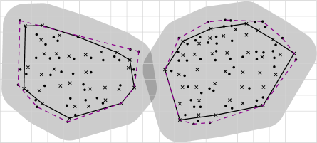
  Figure 5: The crossed points are the points of $\widehat{P}$. The left gray region is $\widetilde{P}_{1}$ and the right gray region is $\widetilde{P}_{2}$. The left dashed polygon is the convex hull of $P_{1}$ and the right dashed polygon is the convex hull of $P_{2}$.

  First, note that $\mathrm{per}(\widehat{P}_{1})+\mathrm{per}(\widehat{P}_{2})\leqslant\mathrm{per}(P_{1}^{*})+\mathrm{per}(P_{2}^{*})$ since $\widehat{P}\subseteq P$. For $i=1,2$, let $\widetilde{P}_{i}$ consist of all points in the plane (not only points in $P$) within a distance of at most $c\sqrt{2}$ from $\mbox{\sc ch}(\widehat{P}_{i})$. In other words, $\widetilde{P}_{i}$ is the Minkowksi sum of $\mbox{\sc ch}(\widehat{P}_{i})$ with a disk $D$ of radius $c\sqrt{2}$ centered at the origin; see Fig. 5. Note that if $p\in\widehat{P}_{i}$, then $q\in\widetilde{P}_{i}$ for any $q\in P\cap C(p)$, since any two points in $C(p)$ are at most $c\sqrt{2}$ apart from each other. Therefore $P_{i}\subset\widetilde{P}_{i}$ and hence $\mathrm{per}(P_{i})\leqslant\mathrm{per}(\widetilde{P}_{i})$. Note also that $\mathrm{per}(\widetilde{P}_{i})=\mathrm{per}(\widehat{P}_{i})+2c\pi\sqrt{2}$. These observations yield

  $$\begin{array}[]{lll}\mathrm{per}(P_{1})+\mathrm{per}(P_{2})&\leqslant&\mathrm{per}(\widetilde{P}_{1})+\mathrm{per}(\widetilde{P}_{2})\\ &=&\mathrm{per}(\widehat{P}_{1})+\mathrm{per}(\widehat{P}_{2})+4c\pi\sqrt{2}\\ &\leqslant&\mathrm{per}(P_{1}^{*})+\mathrm{per}(P_{2}^{*})+4c\pi\sqrt{2}\\ &=&\mathrm{per}(P_{1}^{*})+\mathrm{per}(P_{2}^{*})+4\pi\sqrt{2}\cdot\left(\varepsilon w/(64\pi\sqrt{2})\right)\\ &\leqslant&\mathrm{per}(P_{1}^{*})+\mathrm{per}(P_{2}^{*})+\varepsilon w/16\\ &\leqslant&(1+\varepsilon)\cdot(\mathrm{per}(P_{1}^{*})+\mathrm{per}(P_{2}^{*})).\end{array}$$

  As all the steps can be done in linear time, the time complexity of the algorithm is $O(n+T(n_{\varepsilon}))$ for some $n_{\varepsilon}=O(1/\varepsilon^{2})$.

∎

4 Concluding remarks

We note that in the exact algorithm, for each of the $O(n)$ base squares $\sigma\in S$, the number of values $\mathrm{per}(P(\sigma\cap h))$ that we query is approximately $2\cdot{4\choose 2}\cdot 4500^{2}\approx 2.4\cdot 10^{8}$. Although it is surely possible to modify the algorithm to get smaller constants (to which we made no attempt), we expect that the algorithm will remain impractical.

Consider the degenerate case where all the input points $P$ are on the $x$-axis. Then the minimum-perimeter sum problem reduces to the well-known maximum-gap problem, where the goal is to find the largest difference between two consecutive numbers in sorted order. Lee and Wu [16] gave a lower bound of $\Omega(n\log n)$ for that problem in the algebraic computation tree model, which therefore also holds for the minimum-perimeter sum problem in that model.

The question by Mitchell and Wynters [17] about the existence of sub-quadratic algorithms for the minimum-perimeter maximum, minimum-area sum, and minimum-area maximum problems remain interesting open problems. To our knowledge, the only published algorithm for any of these problems is the $O(n^{4}\log n)$-time algorithm by Bae et al. [6] for the minimum-area sum problem, since the algorithms by Mitchell and Wynters consider line partitions only.

Acknowledgements

This research was initiated when the first author visited the Department of Computer Science at TU Eindhoven during the winter 2015–2016. He wishes to express his gratitude to the other authors and the department for their hospitality.

References

- [1] M. Abrahamsen, A. Adamaszek, K. Bringmann, V. Cohen-Addad, M. Mehr, E. Rotenberg, A. Roytman, and M. Thorup. Fast Fencing. In Proc. 50th Annu. ACM SIGACT Symp. Theory Comput. (STOC), pages 564–573, 2018.
- [2] M. Abrahamsen, M. de Berg, K. Buchin, M. Mehr and A.D. Mehrabi. Minimum perimeter-sum partitions in the plane. In Proc. 33rd ACM Symp. Comput. Geom. (SoCG), pages 4:1–4:15, 2017.
- [3] P.K. Agarwal and M. Sharir. Efficient algorithms for geometric optimization. ACM Comput. Surv. 30(4): 412–458, 1998.
- [4] E.M. Arkin, S. Khuller, and J.S.B. Mitchell. Geometric knapsack problems. Algorithmica 10(5): 399–427, 1993.
- [5] T. Asano, B. Bhattacharya, M. Keil, and F. Yao. Clustering algorithms based on minimum and maximum spanning trees. In Proc. 4th ACM Symp. Comput. Geom. (SoCG), pages 252–257, 1988.
- [6] S.W. Bae, H.-G. Cho, W. Evans, N. Saeedi, and C.-S. Shin. Covering points with convex sets of minimum size. Theor. Comput. Sci., in press, 2016.
- [7] M. de Berg, O. Cheong, M. van Kreveld, and M. Overmars. Computational Geometry: Algorithms and Applications (3rd edition). Springer-Verlag, 2008.
- [8] V. Capoyleas, G. Rote, G. Woeginger. Geometric clusterings. J. Alg. 12(2): 341–356, 1991.
- [9] T.M. Chan. More planar two-center algorithms. Comput. Geom. Theory Appl. 13(2): 189–198, 1999.
- [10] O. Devillers and M.J. Katz. Optimal line bipartitions of point sets. Int. J. Comput. Geom. Appl. 9(1): 39–51, 1999.
- [11] Z. Drezner. The planar two-center and two-median problems. Transp. Sci. 18(4): 351–361, 1984.
- [12] D. Eppstein. Faster construction of planar two-centers. In Proc. 8th ACM-SIAM Symp. Discr. Alg. (SODA), pages 131–138, 1997.
- [13] S. Har-Peled. Geometric approximation algorithms. Mathematical surveys and monographs, Vol. 173. American Mathematical Society, 2011.
- [14] J. Hershberger. Minimizing the sum of diameters efficiently. Comput. Geom. Theory Appl. 2(2): 111–118, 1992.
- [15] J.W. Jaromczyk and M. Kowaluk. An efficient algorithm for the Euclidean two-center problem. In Proc. 10th ACM Symp. Comput. Geom. (SoCG), pages 303–311, 1994.
- [16] D.T. Lee and Y.F. Wu. Geometric complexity of some location problems. Algorithmica 1: 193–211, 1986.
- [17] J.S.B. Mitchell and E.L. Wynters. Finding optimal bipartitions of points and polygons. In Proc. 2nd Workshop Alg. Data Struct. (WADS), LNCS 519, pages 202–213, 1991. Full version available at http://www.ams.sunysb.edu/~jsbm/.
- [18] E. Oh and H.-K. Ahn. Polygon Queries for Convex Hulls of Points. In Proc. 24th Int. Comput. Comb. Conf. (COCOON), pages 143–155, 2018.
- [19] J. Rokne, S. Wang, and X. Wu. Optimal bipartitions of point sets. In Proc. 4th Canad. Conf. Comput. Geom. (CCCG), pages 11–16, 1992.
- [20] M. Segal. Lower bounds for covering problems. J. Math. Modell. Alg. 1(1): 17–29, 2002.
- [21] M. Sharir. A near-linear algorithm for the planar 2-center problem. Discr. Comput. Geom. 18(2): 125–134, 1997.