Thermoelectric Transport through SU(N) Kondo Impurity

Abstract

We investigate thermoelectric transport through a SU(N) quantum impurity in the Kondo regime. The strong coupling fixed point theory is described by the local Fermi-liquid paradigm. Using Keldysh technique we analyse the electric current through the quantum impurity at both finite bias voltage and finite temperature drop across it. The theory of a steady state at zero-current provides a complete description of the Seebeck effect. We find pronounced non-linear effects in temperature drop at low temperatures. We illustrate the significance of the non-linearities for enhancement of thermopower by two examples of SU(4) symmetric regimes characterized by a filling factor $m$: i) particle-hole symmetric at $m$$=$$2$ and ii) particle-hole non-symmetric at $m$$=$$1$. We analyse the effects of potential scattering and coupling asymmetry on the transport coefficients. We discuss connections between the theory and transport experiments with coupled quantum dots and carbon nanotubes.

Introduction. Recent progress in understanding of thermoelectric phenomena on the nanoscale stimulated both new experiments Jezouin et al. (2016); Iftikhar et al. (2015); Jezouin et al. (2013) and development of new theoretical approaches to this problem (see e.g. Benenti et al. (2017) for review). One of the fundamental properties of the quantum transport through nano-sized objects (quantum dots (QD), carbon nanotubes (CNT), quantum point contacts (QPC) etc) is associated with the charge quantization Blanter and Nazarov (2009). It offers a very efficient tool for the quantum manipulation of the single-electron devices being building blocks for quantum information processing. The universality of the heat flows in the quantum regime, scales of the quantum interference effects and limits of the tunability are the central questions of the new emergent field of the quantum heat transport Jezouin et al. (2016); Iftikhar et al. (2015); Jezouin et al. (2013); Molenkamp et al. (1990); vanHouten et al. (1992); Scheibner et al. (2005). Besides, the effects of strong electron correlations and resonance scattering become very pronounced at low temperatures and can be measured with high controllability (e.g. external electric and magnetic fields, geometry, temperature etc) of the semiconductor nano-devices. Therefore, investigation of the quantum effects and influence of strong correlations and resonance scattering on the heat transport (both experimentally and theoretically) is one of the cornerstones of quantum electronics.

As follows from the Fermi-liquid (FL) theory, the thermoelectric power (Seebeck effect) of bulk metals is directly proportional to the temperature $T$ and inversely proportional to the Fermi energy $\varepsilon_{F}$ Zlatic and Monnier (2014). The resonance scattering on a quantum impurity, however, dramatically enhances this effect due to the emergence of new quasiparticle resonances at the Fermi level described by the Kondo effect Noziéres (1974); Nozieres and Blandin (1980); Hewson (1993). The contribution to the Seebeck effect proportional to the concentration of impurities at low $T$, as a result, scales as $T/T_{K}$ Hewson (1993); Zlatic and Monnier (2014) where $T_{K}$ is a characteristic energy defining the width of the Kondo resonance, the Kondo temperature (Fig. 1). The Kondo effect in nano-devices is key for enhancing the thermoelectric transport coefficients Scheibner et al. (2005). The tunable thermo-transport through nano-devices controlling the heat flow is needed for efficient operation of quantum circuits elements: single-electron transistors, quantum diodes etc to perform controllable heat guiding.

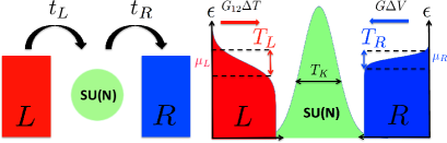
Figure 1: (Color online) Left panel: cartoon for the tunneling $t_{L/R}$ through the SU(N) quantum impurity (see the main text). Right panel: Fermi distribution functions of the left (hot) and right (cold) leads at temperatures $T_{L/R}$ and chemical potential $\mu_{L/R}$. The thermo-voltage $\Delta V=|\mu_{R}-\mu_{L}|/e$ is applied to achieve the steady state with zero net current across the impurity. Left (red)/right (blue) arrows show directions of thermo- and electric- currents. Resonance Kondo peak of width $T_{K}$ in DoS is shown by the green color.

The Kondo effect has been observed in the experiments on the semiconductor quantum dots and the single wall carbon nanotubes Goldhaber-Gordon et al. (1998); Cronenwett et al. (1998); Nygåard et al. (2000); Schröer et al. (2006). The effect manifests itself by complete screening of spin of the quantum impurity and, as a result, the FL behaviour in the strong coupling (low temperatures) regime Noziéres (1974); Nozieres and Blandin (1980); Affleck and Ludwig (1993). Here we use the local FL paradigm Mora (2009); Vitushinsky et al. (2008); Mora et al. (2008, 2009, 2015); LeHur et al. (2007); Hörig et al. (2014); Hanl et al. (2014) which is a powerful tool for the description of thermodynamic and transport properties of quantum impurity in the strong coupling regime. It has also been applied recently for explanation of ”0.7-anomaly” in QPCs Rejec and Meir (2006); Bauer et al. (2013a). The $s$$=$$1/2$ SU(2) Kondo impurity physics arises at the half-filled particle-hole (PH) symmetric regime. We refer to ”electrons” as quasiparticles above $\varepsilon_{F}$ and ”holes” as the excitations below $\varepsilon_{F}$. The PH symmetry, being responsible for the enhancement of the electric conductance, suppresses however the thermo-electric transport: the thermo- current carried by electrons is completely compensated by heat current carried by holes challenging however to investigate Kondo models in the regime away from PH-symmetry. To achieve appreciable thermopower, the occupation factor of the quantum impurity should be integer (Coulomb blockade valleys Blanter and Nazarov (2009)), while the particle-hole symmetry should be lifted. Such properties are generic for the SU(N) Kondo models with the filling factors different from $1/2$.

The SU(N) Kondo physics with $N$$=$$4$ is experimentally realized in CNTs Jarillo-Herrero et al. (2005); Makarovski et al. (2007a, b); Ferrier et al. (2016) and double QDs Keller et al. (2014). The SU(N) Kondo model has also been proposed to investigate in ultra-cold gases experiments Bauer et al. (2013b); Nishida (2013). There are several theoretical suggestions for realization of SU(N) Kondo physics with $N$$=$$3$ Nishida (2013, 2016) $N$$=$$6$ Kuzmenko et al. (2016) and $N$$=$$12$ reported in Kuzmenko and Avishai (2014). While the electron transport through SU(N) Kondo impurity is well understood theoretically LeHur et al. (2004); Lopez et al. (2005); Schmid et al. (2015); Mora et al. (2009), the thermo-electric transport in the Kondo regime remains challenging Sakano and Kawakami (2006); Sakano et al. (2007); Roura-Bas et al. (2012); Azema et al. (2012); Dorda et al. (2016).

In this Letter we present a full fledged theory for the Seebeck effect of SU(N) Kondo model for the strong coupling regime $T$$\ll$$T_{K}$. Our approach is based on real time out-of equilibrium Keldysh calculations. We used the local Fermi-liquid paradigm for constructing a perturbative expansion for the electric current around the strong coupling fixed point of the model. We illustrate the thermoelectric properties of the SU(N) Kondo model on two particular examples, namely, $N$$=$$4$ with the filling factors $1/4$ and $1/2$. We compute the thermoelectric power for arbitrary temperature drop between the electron reservoirs and discuss the significance of non-linear effects in temperature drop.

Setup. We consider an SU(N) quantum impurity (such as a CNT or coupled QDs) sandwiched between two leads (Fig. 1). The model geometry resembles the experimental setup Scheibner et al. (2005). The temperature of the drain electrode (R) is taken as the reference temperature of the system. The temperature of the source electrode (L) is controlled by the Joule heat released due to the finite current flowing along the lead Scheibner et al. (2005). Thus, the temperature drop $\Delta T$ is fixed for all measurements. The bias voltage $\Delta V$ is applied between the source and the drain in order to stop the thermo-current (Fig. 1 right panel):

$$I=0=G(T)\Delta V+G_{12}(T)\Delta T.$$ (1)

The differential thermoelectric power is defined at the total current across the impurity tuned to zero:

$$S(T)=\left.-\lim_{\Delta T\to 0}\frac{\Delta V}{\Delta T}\right|_{I=0}=\frac{G_{12}(T)}{G(T)},$$ (2)

$G$$=$$\partial{I}$$/$$\partial{\Delta V}$$\left.\right|_{\Delta T=0}$ is the electric conductance and $G_{12}$$=$$\partial{I}$$/$$\partial{\Delta T}$$\left.\right|_{\Delta V=0}$ is the thermoelectric coefficient.

Model. The tunneling of electrons through the SU(N) quantum impurity (Fig.1 left panel) is described by the Anderson model Mora et al. (2009):

$$\begin{split}H=&\sum_{k\alpha r}\varepsilon_{k}c^{\dagger}_{\alpha kr}c_{\alpha kr}+\sum_{r}\epsilon_{0}d^{\dagger}_{r}d_{r}\\ &+\sum_{r<r^{\prime}}Ud^{\dagger}_{r}d_{r}d^{\dagger}_{r^{\prime}}d_{r^{\prime}}+\sum_{k\alpha r}t_{\alpha}d^{\dagger}_{r}c_{\alpha kr}+H.c.\end{split}$$ (3)

Here $d_{r}$ annihilates an electron in the dot level $\epsilon_{0}$ with orbitals $r=1,2,...N$, $c_{\alpha kr}$ annihilates a conduction electron with the momentum $k$ and orbital $r$ in the leads $\alpha=L,R$ and $U$ is the Coulomb repulsion (charging) energy in the dot, $t_{\alpha}$ is lead-dot tunneling and $\varepsilon_{k}=\epsilon_{k}-\varepsilon_{F}$ is the linearized conductance electron’s dispersion. We assume that the charging energy $U$ is the largest energy scale of the model and therefore take into account only ”last” occupied state. We project out the charge states by applying the Schrieffer-Wolff transformation Schrieffer and Wolf (1966). As a result we obtain the effective SU(N) Kondo model describing the physics at the weak coupling $T$$\gg$$T_{K}$ limit:

$$\mathcal{H}_{K}=J_{K}^{\alpha\beta}\left(\bf{c^{\dagger}_{\alpha}\lambda^{\mu}c_{\beta}}\right)\left(\bf{d^{\dagger}\Lambda^{\mu}d}\right),$$ (4)

where $\bf{c^{\dagger}}$=$(c^{\dagger}_{1},....,c^{\dagger}_{N})$ is a row vector of the electron states in the leads and $\bf{d^{\dagger}}$=$(d^{\dagger}_{1},....,d^{\dagger}_{N})$ represents the local states in the dot. The $SU(N)$ generators $\bf{\lambda^{\mu}}$ and $\bf{\Lambda^{\mu}}$ for $\mu=1,2,....N^{2}-1$ are traceless $N\times N$ Hermitian matrices of the fundamental representation, satisfying the commutation relations $\left[\bf{\lambda^{\mu}},\bf{\lambda^{\nu}}\right]$$=$$if^{\mu\nu\rho}\bf{\lambda^{\rho}}$ where $f^{\mu\nu\rho}$ is the set of fully anti-symmetric structure factors. As a last step we diagonalize the matrix $J_{K}^{\alpha\beta}$$\sim$$|$$t_{\alpha}$$t_{\beta}$$|$$/U$ in the sub-space of two leads $\alpha$,$\beta$$=$$L$,$R$ performing the Glazman-Raikh rotation Glazman and Raikh (1988); Ng and Lee (1988); Pustilnik and Glazman (2004). Similarly to the SU(2) Kondo model, the anti-symmetric combination of the electron states in the leads $a^{\dagger}=(c^{\dagger}_{L}-c^{\dagger}_{R})/\sqrt{2}$ is fully decoupled from the Hamiltonian while the symmetric combinations $b^{\dagger}=(c^{\dagger}_{L}+c^{\dagger}_{R})/\sqrt{2}$ remains coupled to the quantum impurity (without loss of generality we present here the results for symmetric $t_{L}$$=$$t_{R}$ dot-lead coupling; general equations for arbitrary coupling are presented in Supplemental Materials Karki and Kiselev ).

The FL Hamiltonian describing the strong coupling $T$$\ll$$T_{K}$ regime is obtained by applying the standard point-splitting procedure to $:\left(\bf{b^{\dagger}\lambda^{\mu}b}\right)\cdot\left(\bf{b^{\dagger}\lambda^{\mu}b}\right):$ (see Affleck and Ludwig (1993) for the details), $H_{FL}$$=$$H_{0}$$+$$H_{\alpha}$$+$$H_{\phi}$ :

$$H_{0} = \nu\sum_{r}\int_{\varepsilon}\varepsilon\left[a^{\dagger}_{\varepsilon r}a_{\varepsilon r}+b^{\dagger}_{\varepsilon r}b_{\varepsilon r}\right]$$ (5)

$$H_{\alpha} = -\sum_{r}\int_{\varepsilon_{1-2}}\left[\frac{\alpha_{1}}{2\pi}(\varepsilon_{1}+\varepsilon_{2})+\frac{\alpha_{2}}{4\pi}(\varepsilon_{1}+\varepsilon_{2})^{2}\right]b^{\dagger}_{\varepsilon_{1}r}b_{\varepsilon_{2}r}$$

$$H_{\phi} = \sum_{r<r^{\prime}}\int_{\varepsilon_{1-4}}\left[\frac{\phi_{1}}{\pi\nu}+\frac{\phi_{2}}{4\pi\nu}\left(\sum^{4}_{i=1}\varepsilon_{i}\right)\right]:b^{\dagger}_{\varepsilon_{1}r}b_{\varepsilon_{2}r}b^{\dagger}_{\varepsilon_{3}r^{\prime}}b_{\varepsilon_{4}r^{\prime}}:.$$

The Kondo floating paradigm Noziéres (1974); Nozieres and Blandin (1980); Affleck and Ludwig (1993); Mora (2009); Vitushinsky et al. (2008); Mora et al. (2008, 2009, 2015); LeHur et al. (2007); Hörig et al. (2014); Hanl et al. (2014) leads to the following FL identities: $\alpha_{1}$$=$$($$N$$-$$1$$)\phi_{1}$ and $\alpha_{2}$$=$$($$N$$-$$1$$)\phi_{2}/4$, $\nu$ is the density of states at $\varepsilon_{F}$. The connection between $\alpha_{1}$ and $\alpha_{2}$ is given by the Bethe ansatz Mora et al. (2009). We use $\alpha_{1}$$=$$1/T_{K}$ as the definition of the Kondo temperature Pustilnik and Glazman (2004).

Charge Current. The current operator at position $x$ is expressed in terms of first-quantized operators $\psi$ attributed to the linear combinations of the Fermi operators in both leads

$$\hat{I}(x)=\frac{\hbar e}{2mi}\sum_{r}\left[\psi^{\dagger}_{r}(x)\partial_{x}\psi_{r}(x)-\partial_{x}\psi^{\dagger}_{r}(x)\psi_{r}(x)\right].$$ (6)

For the expansion of Eq.(6), we choose the basis of scattering states that includes completely elastic and Hartree terms Mora et al. (2009) to get it in compact form:

$$\hat{I}=\frac{e}{2\nu h}\sum_{r}\left[a^{\dagger}_{r}(x)b_{r}(x)-a^{\dagger}_{r}(-x)Sb_{r}(-x)+H.c.\right],\;\;\;$$ (7)

where $a_{r}(x)$$=$$\sum_{k}$$a_{kr}$$e^{ikx}$, $b_{r}(x)$$=$$\sum_{k}$$b_{kr}$$e^{ikx}$, $Sb_{r}(x)$$=$$\sum_{k}$$S_{k}b_{kr}$$e^{ikx}$ and the $N$$\times$$N$ $S$-matrix is expressed in terms of a phase shift $\delta$$($$\varepsilon_{k}$$)$ as $S_{k}$$=e^{2i\delta(\varepsilon_{k})}$.

Elastic current. Calculation of the expectation value of (7) in the absence of interactions is equivalent to use the Landauer-Büttiker formalism Blanter and Nazarov (2009):

$$I_{el}=\frac{Ne}{h}\int^{\infty}_{-\infty}d\varepsilon\mathcal{T}(\varepsilon)\Delta f(\varepsilon),$$ (8)

where $\Delta f(\varepsilon)$$=$$f_{L}(\varepsilon)$$-$$f_{R}(\varepsilon)$, $f_{L/R}$ are Fermi distribution functions of L/R leads; $\mu_{L}$$-$$\mu_{R}$$=$$e\Delta$$V$$\ll$ $T_{K}$ are the chemical potentials, $T_{R}$$=$$T$ is the reference temperature and $T_{L}$$=$$T$$+$$\Delta T$ (Fig.1 right panel). The energy dependent transmission $\mathcal{T}(\varepsilon)$$=$$\sin^{2}\left[\delta(\varepsilon)\right]$. Following Ref. Mora et al. (2009), we Taylor-expand the phase shift for all flavours $r$ in the presence of voltage bias $e\Delta V$ and temperature drop $\Delta T$ as $\delta_{r}(\varepsilon)=\delta_{0}+\alpha_{1}\varepsilon+\alpha_{2}\left(\varepsilon^{2}-{\cal A}\right)$, where ${\cal A}=\left[\frac{(e\Delta V)^{2}}{4}+\frac{(\pi T)^{2}}{3}+\frac{\pi^{2}T\Delta T}{3}\right]$ and $\delta_{0}$$=$$\pi$$m$$/N$ for the quantum impurity’s occupation $m$$=$$1$$,...,$$N$$-$$1$. The zero energy transmission is given by $\mathcal{T}_{0}$$=$$\sin^{2}\delta_{0}$. Using the above equation for the phase shift $\delta_{r}$ we expand the current up to the second order in $T$$/$$T_{K}\ll 1$ to get the elastic contribution. The linear response result is:

$$\frac{I_{el}}{Ne/h} = \left[{\color[rgb]{0,0,0}\sin^{2}\delta_{0}}+\frac{\alpha^{2}_{1}}{3}(\pi T)^{2}\cos 2\delta_{0}\right]e\Delta V$$ (9)

$$- \left[\frac{\alpha_{1}}{3T}(\pi T)^{2}\sin 2\delta_{0}\right]\Delta T.$$

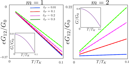
Figure 2: (Color online) Main frame: Thermoelectric coefficient $G_{12}$ as a function of the reference temperature $T$$=$$T_{R}$ at different values of potential scattering $\delta_{P}$. Insert: differential conductance $G$ as a function of $T$ for $\delta_{P}$$=$$0.3$. The legend is shown on the left panel. Solid lines - numerical solution obtained from (1) with (S6-S7, S11-S12) Karki and Kiselev . Dashed lines - analytical solution given by (15, 16). Solid and dashed lines are almost indistinguishable.

Inelastic current. The inelastic contribution to the current is computed using the non-equilibrium Keldysh formalism Keldysh (1965):

$$\delta I_{in}=\langle T_{{}_{C}}\hat{I}(t)e^{-i\int dt^{\prime}H_{\phi}(t^{\prime})}\rangle,$$ (10)

where $C$ denotes the double side $\eta=\pm$ Keldysh contour Keldysh (1965). Here $T_{C}$ is the time ordering operator on a contour and the average is performed with the Hamiltonian $H_{0}$ whereas the contribution from $H_{\alpha}$ is already accounted in $I_{el}$. As discussed in detail in Ref. Mora et al. (2015), the second order interaction correction to the current is expressed in terms of the self-energies

$$\delta I_{in}=\mathcal{S}\int^{\infty}_{-\infty}\frac{d\varepsilon}{2\pi}\left(\Sigma^{-+}(\varepsilon)-\Sigma^{+-}(\varepsilon)\right)i\pi\nu\Delta f(\varepsilon),\;\;\;\;$$ (11)

we used the notation: $\mathcal{S}=\frac{N(N-1)e\pi}{h}\cos 2\delta_{0}$. The self-energies in Eq.(11) are defined in terms of the Green’s functions as: $\Sigma^{\eta_{1},\eta_{2}}(t)=\left(\frac{\phi_{1}}{\pi\nu^{2}}\right)^{2}\sum_{k_{1},k_{2},k_{3}}G^{\eta_{1},\eta_{2}}_{bb}(k_{1},t)G^{\eta_{2},\eta_{1}}_{bb}(k_{2},-t)G^{\eta_{1},\eta_{2}}_{bb}(k_{3},t)$. The local Green’s functions of $aa$$/$$bb$ fermions and the mixed $ab$ fermions in real-time are given by

$$\mathcal{G}_{\pm}(t)=-\frac{\pi\nu}{2}\left[\frac{T_{L}e^{-i\mu_{L}t}}{\sinh(\pi T_{L}t)}\pm\frac{T_{R}e^{-i\mu_{R}t}}{\sinh(\pi T_{R}t)}\right],$$ (12)

with $\mathcal{G}_{+}(t)$$=$$G^{+-}_{aa/bb}(t)$ and $\mathcal{G}_{-}(t)$$=$$G_{ba/ab}(t)$$=$$i\pi\nu\Delta f(t)$. Computing the integrals in the presence of the finite bias voltage and finite temperature drop one gets:

$$\Sigma^{-+}(\varepsilon)-\Sigma^{+-}(\varepsilon)=$$

$$\frac{\phi^{2}_{1}}{i\pi\nu}\left[\frac{3}{4}(e\Delta V)^{2}+\frac{\Delta T}{T}(\pi T)^{2}+\varepsilon^{2}+(\pi T)^{2}\right].$$ (13)

In the limit $\Delta$$T$$\to$$0$, $\Delta$$f(\varepsilon)$$=$$-$$($$\Delta$$T$$\cdot\varepsilon$$/$$T$$)$$\cdot\partial f/\partial\varepsilon$ and the FL self-energies, being even functions of $\varepsilon$, do not contribute to the thermo-current at $\Delta V$$=$$0$. Therefore, the thermoelectric coefficient $G_{12}$ at $\Delta T$$\to$$0$ is fully determined by elastic processes . The linear response inelastic contribution to the current at $\Delta$$T$$=0$ reads

$$\frac{\delta I_{in}}{Ne/h}=\left[\frac{2}{3}\left(\pi T\right)^{2}\left(N-1\right)\phi^{2}_{1}\cos 2\delta_{0}\right]e\Delta V.$$ (14)

The equation for the total current beyond the linear response is cumbersome and given in Supplemental Materials Karki and Kiselev . Finally, the differential conductance $G$ and differential thermo-electric coefficient $G_{12}$ are give by:

$$G(T) = G_{0}\left[{\color[rgb]{0,0,0}\sin^{2}\delta_{0}}+\frac{\alpha^{2}_{1}}{3}\frac{N+1}{N-1}(\pi T)^{2}\cos 2\delta_{0}\right],\;\;\;$$ (15)

$$G_{12}(T) = -G_{0}\left[\frac{\alpha_{1}}{3e}\pi^{2}T\sin 2\delta_{0}\right],$$ (16)

where $G_{0}=Ne^{2}/h$ is the unitary conductance.

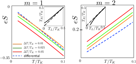
Figure 3: (Color online) Main frame: Thermoelectric power $S$ as a function of the reference temperature $T$$=$$T_{R}$; blue dashed curve: differential $S$ given by (2) with (15, 16); solid curves correspond to $S$ defined under zero-current condition by (1) with (S6-S7, S11-S12) Karki and Kiselev at different values of $\Delta T$ (see the legend); $\delta_{P}$$=$$0.3$. Insert: evolution of the zero current steady state as a function of the temperatures of L-R leads at finite voltage $e$$\Delta$$V$$/$$T_{K}$$=0.02$.

Potential scattering. As is seen from (16), the $G_{12}$ at given reference temperature $T$ in linear response is proportional to $\sin 2\delta_{0}$. For the particle-hole symmetric (PHS) case in the absence of potential scattering $m$$=$$N/2$ (we assume $N$ even), $\delta_{0}$$=$$\pi/2$ and both $G_{12}$ and the thermoelectric power are zero - the particle thermo current exactly compensates the hole thermo current (Fig. 2 right panel, blue curve). The potential scattering explicitly breaks the PH symmetry. It can be accounted by replacement of $\delta_{0}$ by $\tilde{\delta}_{0}$$=$$\delta_{0}$$+$$\delta_{P}$, $\delta_{P}$$\ll$$\delta_{0}$. As a result, the finite $G_{12}$ and thermopower arises. The results of calculations obtained from the zero-current conditions for SU(4) quantum impurity are illustrated on Fig. 2. First, for the case of singly occupied quantum impurity $m$$=$$1$ (Fig. 2 left panel) $\delta_{0}$$=$$\pi/4$ and the PH symmetry is explicitly broken. At zero potential scattering inelastic effects associated with the finite bias voltage vanish and the thermoelectric power is completely defined by elastic processes. The effect of potential scattering is two-fold: i) it detunes $G_{12}$ from it’s maximal value and ii) it results in finite-temperature inelastic corrections to the conductance (see the Fig. 2 insert). For the PHS case of double occupation $m$$=$$2$ (Fig. 2 right panel) $\delta_{0}$$=$$\pi/2$. Therefore the finite potential scattering results in finite $G_{12}$ and differential thermopower $S$ is proportional to $\sin 2\delta_{P}$. Crossover between $m$$=$$2$ SU(4) and $m$$=$$1$ SU(2) has been studied recently experimentally Ferrier et al. (2017). Note that the current across the dot symmetrically coupled to the leads contains only odd powers of the voltage both for the PHS $m$$=$$2$ and the PH-non-symmetric (PHN) $m$$=$$1$ cases.

Seebeck effect. In the limit $T$$\rightarrow$$0$ the differential thermopower is given by

$$S(T)=-2eL_{0}T\cot\tilde{\delta}_{0}\left.\frac{\partial\tilde{\delta}(\varepsilon)}{\partial\varepsilon}\right|_{\varepsilon=0}=-\frac{\pi\gamma T}{e}\cot\tilde{\delta}_{0},\;\;\;\;\;\;$$ (17)

where $L_{0}$$=$$\pi^{2}$$/$$(3e^{2})$ is the Lorentz number and $\gamma$$=$$2$$\pi$$\alpha_{1}/3$$\sim$$1$$/T_{K}$ in accordance with the FL theory Hewson (1993).

The thermopower measurements Scheibner et al. (2005) refer however not to the differential Seebeck effects (see Fig. 1). Since there were no independent measurements of $T_{L}$ and $T_{R}$, the temperature drop was estimated from the Joule heat. It appeared that the $\Delta T$ was finite and not fulfilling the condition $|\Delta T|$$\ll$$T_{R}$. To demonstrate the significance of non-linear effects associated with finite temperature drop we show on Fig. 3 the thermopower of SU(4) model computed by two different methods: i) the dashed blue line stands for the differential thermopower $S(T)$$=$$G_{12}$$/$$G$ where $G_{12}$ is obtained at zero voltage drop while $G$ is calculated at equal temperatures of the leads; ii) the solid lines corresponds to $S$$=$$-$$\Delta$$V$$/$$\Delta$$T$ resembling the experimental situation in Scheibner et al. (2005) : the temperature drop is fixed $\Delta$$T$$/$$T_{K}$$=0.05$ (red) $0.025$ (green) $0.01$ (orange) and the thermo-voltage is obtained from the zero current condition. As one can see, at small reference temperatures ”finite $\Delta T$” thermopower always overshoots the differential $S$. The effect is more pronounced in PHS regime . This observation can explain the thermo-voltage offset observed in the experiment Scheibner et al. (2005) in the Kondo limit of SU(2) quantum impurity (PHS regime). According to our calculations this offset is associated with a non-linear $\Delta T$ dependence of the current at low reference temperatures (see Fig. 3 inserts). We suggest to check this statement experimentally by performing Seebeck effect measurements varying the temperature in the ”hot” lead.

Coupling asymmetry. The effect of coupling asymmetry $t_{L}$$\neq$$t_{R}$ in (3) manifests itself in the following way: for broken PH-symmetry case it results in an asymmetric I-V curve due to a contribution to the current quadratic in voltage which, in turn, depends linearly on the coupling asymmetry. For both PHS and PHN cases the coupling asymmetry results in i) renormalization of the elastic contribution to the charge current (see Karki and Kiselev Eq. S5); ii) renormalization of the Kondo temperature due to tunneling rates asymmetry Karki and Kiselev ; and iii) renormalization of the coefficient in front of the term cubic in voltage. The magnitude of current is suppressed by the coupling asymmetry. Besides, it also affects the thermo-current. However, this effect is proportional to $\Delta$$V$$\cdot\Delta T$ and therefore beyond the linear response theory (see the Supplemental Materials Karki and Kiselev for details).

Peltier effect. In order to compute other thermo-electric coefficients, e.g. Peltier effect, one needs to define and compute the heat current. To proceed with full fledged Keldysh calculations one can e.g. deal with the Luttinger ”gravitational potential” approach Luttinger (1964); Shastry (2009); Eich et al. (2014). Such a theory would access the effects non-linear in $\Delta T$ Karki and Kiselev (2017). In the linear response theory the Peltier coefficient $\Pi$$($$T)$ can be calculated using the transport integrals method (see, e.g. Costi and Zlatić (2010) for details) based on calculation of different momenta of the single-particle lifetime $\tau$$($$\epsilon$,$T)$ (see the Supplemental materials Karki and Kiselev ) and is related to the thermopower by the Onsager’s relation $\Pi(T)$$=$$S$$($$T$$)$$\cdot T$.

Summary. The full fledged theory based on Keldysh out-of equilibrium calculations of the electric current is constructed for the SU(N) Kondo quantum impurity subject to a finite bias voltage and a finite temperature drop. The transport coefficients: conductance $G$, thermoelectric coefficient $G_{12}$ and thermopower $S$ are computed under condition of zero-current state for the strong-coupling regime of the quantum impurity. It is shown that pronounced non-linear effects in temperature drop influence the transport coefficients at the low-temperature limit. These effects are likely sufficient to resolve the experimental puzzle of the thermo-transport through the Kondo impurity at the strong coupling.
Acknowledgement. We acknowledge fruitful discussions with Jan von Delft, Laurens W. Molenkamp and Christophe Mora. We are grateful to Yu. Galperin and S. Ludwig for careful reading the manuscript, comments and suggestions. This work was finalized at Aspen Center for Physics, which is supported by National Science Foundation grant PHY-1607611 and was partially supported (MK) by a grant from the Simons Foundation.
Note added. While completing this work, a paper Sierra et al. (2017) appeared where the significance of non-linear effects in temperature drop on the temperature-driven current through SU(2) quantum impurity has been reported.

Supplemental Materials

This Supplemental Materials contains additional information about the charge current beyond the linear response theory and connections between the full fledged calculations performed using Kedlysh out-of-equilibrium approach and the results derived by means of the transport integrals method.

I Electric current beyond the linear response

I.1 Coupling asymmetry

If the quantum impurity is coupled to the leads with arbitrary coupling, the new variables ($a$ and $b$) entering the FL Hamiltonian (Thermoelectric Transport through SU(N) Kondo Impurity) are defined by Glazman-Raikh rotation Glazman and Raikh (1988); Ng and Lee (1988); Pustilnik and Glazman (2004) as follows:

$$\left(\begin{array}[]{c}b_{kr}\\ a_{kr}\\ \end{array}\right)=\left(\begin{array}[]{cc}\cos\theta&\sin\theta\\ \sin\theta&-\cos\theta\\ \end{array}\right)\left(\begin{array}[]{c}c_{Lkr}\\ c_{Rkr}\\ \end{array}\right),$$ (S1)

where $\tan$$\theta$$=$$|t_{R}/t_{L}|$ is given by the ratio of tunnel lead-dot matrix elements Pustilnik and Glazman (2004) of the Hamiltonian (3). The symmetric coupling corresponds to $\theta$$=$$\pi/4$. We introduce the parameter $\mathcal{C}$$=$$\cos 2\theta$$=$$(\Gamma_{L}-\Gamma_{R})$$/$$(\Gamma_{L}+\Gamma_{R})$ to characterize the asymmetry of the dot-lead coupling; $\Gamma_{\alpha}$$=$$\pi$$\nu$$N$$|t_{\alpha}|^{2}$ is intrinsic total local level width associated with the tunneling from/to the reservoirs (we assume that tunnel matrix elements are the same for all orbitals/flavours).

I.2 Phase shift

The phase shift expression in the presence of the finite voltage bias $e\Delta V$, finite temperature drop across the impurity $\Delta T$ is given by the equation Mora et al. (2009):

$$\delta(\varepsilon)=\delta_{0}+\alpha_{1}\varepsilon+\alpha_{2}\varepsilon^{2}-\frac{N-1}{4}\phi_{2}\cdot{\cal A},$$ (S2)

where

$${\cal A}=\frac{1}{6}\left[(\pi T_{L})^{2}(1+\mathcal{C})+(\pi T_{R})^{2}(1-\mathcal{C})+\frac{3}{2}(1-\mathcal{C}^{2})(e\Delta V)^{2}\right].$$ (S3)

The FL identities $\alpha_{1}=(N-1)\phi_{1}$ and $\alpha_{2}=1/4(N-1)\phi_{2}$ follow from the Kondo floating paradigm Noziéres (1974); Mora et al. (2009); Mora (2009). The exact relation between $\alpha_{1}$ and $\alpha_{2}$ is given by the Bethe-Ansatz solution Mora et al. (2009); Mora (2009):

$$\frac{\alpha_{2}}{\alpha^{2}_{1}}=\frac{N-2}{N-1}\frac{\Gamma(1/N)\tan(\pi/N)}{\sqrt{\pi}\Gamma\left(\frac{1}{2}+\frac{1}{N}\right)}\cot\delta_{0}.$$ (S4)

Here $\Gamma(x)$ is the Euler’s gamma-function.

I.3 Elastic current

The elastic contribution to the charge current is performed by averaging the current with $H_{\alpha}$ of (Thermoelectric Transport through SU(N) Kondo Impurity) which is equivalent to use of the Landauer-Büttiker formula Blanter and Nazarov (2009) containing the energy dependent transmission coefficient ${\cal T}(\varepsilon)$ computed with the scattering phase (S2, S3):

$$I_{el}=\frac{Ne}{h}\int d\varepsilon{\cal T}(\varepsilon)\Delta f(\varepsilon),\quad{\cal T}(\varepsilon)=\left(1-\mathcal{C}^{2}\right)\sin^{2}[\delta(\varepsilon)].$$ (S5)

Computing integrals with Fermi distribution function we obtain the elastic current:

$$I_{el}=\frac{Ne}{h}\left(1-\mathcal{C}^{2}\right)\left[(\mathcal{T}_{0}-\sin 2\delta_{0}\alpha_{2}\mathcal{A})\mathcal{J}_{0}-\sin 2\delta_{0}\alpha_{1}\mathcal{J}_{1}+(\cos 2\delta_{0}\alpha^{2}_{1}+\sin 2\delta_{0}\alpha_{2})\mathcal{J}_{2}\right],$$ (S6)

where we use short-hand notations:

$$\mathcal{J}_{0} = e\Delta V,\quad\mathcal{J}_{1}=\frac{1}{6}\left[(\pi T_{L})^{2}-(\pi T_{R})^{2}-3(e\Delta V)^{2}\mathcal{C}\right],$$

$$\mathcal{J}_{2} = \frac{e\Delta V}{6}\left[(\pi T_{L})^{2}(1-\mathcal{C)}+(\pi T_{R})^{2}(1+\mathcal{C)}+\frac{1}{2}(e\Delta V)^{2}(1+3\mathcal{C}^{2})\right].$$ (S7)

I.4 Inelastic current

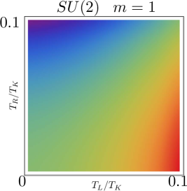
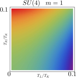
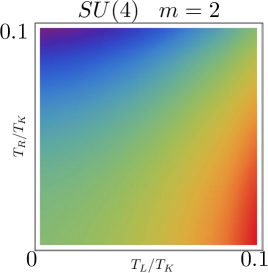
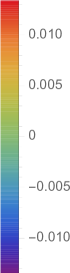
Figure S1: (Color online) Density plot showing the thermo-voltage $e\Delta V/T_{K}$ obtained at the zero-current conditions as a function of the temperatures of L/R contacts. Left panel: SU(2) PH-symmetric Kondo regime $m=1$; central panel: SU(4) PH-non-symmetric Kondo regime $m=1$; right panel: SU(4) PH-symmetric Kondo regime $m=2$; for all plots: $\delta_{P}$$=$$0.3$, $\gamma$$T_{K}=$$0.001$ and $\mathcal{C}=0$.

For computing the inelastic contribution to the current we use the general equation for the self-energies

$$\Sigma^{\eta_{1},\eta_{2}}(t)=\left(\frac{\phi_{1}}{\pi\nu^{2}}\right)^{2}\sum_{k_{1},k_{2},k_{3}}G^{\eta_{1},\eta_{2}}_{bb}(k_{1},t)G^{\eta_{2},\eta_{1}}_{bb}(k_{2},-t)G^{\eta_{1},\eta_{2}}_{bb}(k_{3},t)$$ (S8)

expressed in terms of the fermionic Green’s functions (which replace (12)):

$$G^{+-}_{bb}(t) = -\frac{\pi\nu}{2}\left[\frac{T_{L}(1+\mathcal{C})e^{-i\mu_{L}t}}{\sinh(\pi T_{L}t)}+\frac{T_{R}(1-\mathcal{C})e^{-i\mu_{R}t}}{\sinh(\pi T_{R}t)}\right],$$ (S9)

$$G_{ab/ba}(t) = -\frac{\pi\nu}{2}\sin 2\theta\left[\frac{T_{L}e^{-i\mu_{L}t}}{\sinh(\pi T_{L}t)}-\frac{T_{R}e^{-i\mu_{R}t}}{\sinh(\pi T_{R}t)}\right],$$ (S10)

where $\mu_{L}=\frac{e\Delta V}{2}(1-\mathcal{C})$ and $\mu_{R}=-\frac{e\Delta V}{2}(1+\mathcal{C})$. We also take into account the coefficient $\sin 2\theta$ in front of the definition of the total current in Eq. 6 and $\sin^{2}2\theta$ in front of the inelastic current in Eq. 11.

The inelastic current for symmetrical dot-lead coupling is given by the relation:

$$\delta I_{in}=\frac{N(N-1)e\pi}{2h}\left(\frac{\phi_{1}}{\pi\nu^{2}}\right)^{2}4\cos 2\delta_{0}\left(\frac{\pi\nu}{2}\right)^{4}\times\left\{\left[\mathcal{L}(T_{L},T_{R},z)-\mathcal{L}(T_{L},T_{R},0)\right]-\left[\mathcal{L}(T_{R},T_{L},-z)-\mathcal{L}(T_{R},T_{L},0)\right]\right\},$$ (S11)

where

$$\mathcal{L}(x,y,z)=\int^{+\infty-i\gamma}_{-\infty-i\gamma}\left[\frac{x^{4}}{\sinh^{4}(\pi xt)}+2x^{3}y\frac{e^{izt}}{\sinh^{3}(\pi xt)\sinh(\pi yt)}+x^{2}y^{2}\frac{e^{2izt}}{\sinh^{2}(\pi xt)\sinh^{2}(\pi yt)}\right]dt$$ (S12)

Here we denoted $z$$=$$e\Delta V$ and introduced the point splitting parameter $\gamma$ Affleck and Ludwig (1993); Mora et al. (2009) to regularize the integrals (S12) divergent at $t$$=$$0$. The parameter $\gamma$ is chosen to satisfy the conditions $\gamma$$e\Delta$$V$$\ll 1$, $\gamma$$T$$\ll 1$ and $T_{K}/D$$\ll$$\gamma$$T_{K}$$\ll 1$ Mora et al. (2009) ($D$ is a bandwidth of conduction band, $T\ll T_{K}$, $T_{K}/D\propto\sqrt{(\Gamma_{L}+\Gamma_{R})/D}\exp[-c\cdot U/(\Gamma_{L}+\Gamma_{R})]$, $c\sim 1$).

We show on Fig. S1 the thermo-voltage $\Delta V$ as a function of two temperatures $T_{L}$ and $T_{R}$ of the left-right leads for three important cases discussed in the paper: i) $m=1$ SU(2); ii) $m=1$ SU(4) and iii) $m=2$ SU(4). One can see similarity of the plots i) and iii) describing the broken by potential scattering particle-hole symmetric regimes. The density plot visualises the non-linearity of the thermo-voltage at low compared to $T_{K}$ temperatures.

II Transport Integrals

We illustrate the application of the textbook Zlatic and Monnier (2014); Costi and Zlatić (2010) method of transport integrals to the thermoelectric transport through the SU(N) quantum impurity assuming the symmetric dot-leads coupling for simplicity. The charge and the heat currents in the linear response theory are connected by equations:

$$\left(\begin{array}[]{c}I_{charge}\\ I_{heat}\\ \end{array}\right)=\left(\begin{array}[]{cc}L_{11}&L_{12}\\ L_{21}&L_{22}\\ \end{array}\right)\left(\begin{array}[]{c}\Delta V\\ \Delta T\\ \end{array}\right).$$ (S13)

Differential conductance $G(T)$ and differential thermopower $S(T)$ are defined as follows:

$$G(T) =\lim_{\Delta V\to 0}\left.\frac{I_{charge}}{\Delta V}\right|_{\Delta T=0}=L_{11},$$ (S14)

$$S(T) =-\lim_{\Delta T\to 0}\left.\frac{\Delta V}{\Delta T}\right|_{I_{charge}=0}=L_{12}/L_{11}.$$ (S15)

The coefficients $L_{ij}$ are expressed in terms of the transport integrals (see e.g.Costi and Zlatić (2010) for details of the derivation):

$${\cal I}_{n}(T)=\frac{1}{h}\sum_{\sigma}\int d\varepsilon\cdot\varepsilon^{n}\left(-\frac{\partial f}{\partial\varepsilon}\right)\cdot{\rm Im}\left[-\pi\nu T_{\sigma}(\varepsilon)\right].$$ (S16)

Here $L_{11}=e^{2}{\cal I}_{0}$, $L_{12}=-e{\cal I}_{1}/(2T)$ and $T_{\sigma}$ is a diagonal part of a single-particle T-matrix defined by the Dyson equation Pustilnik and Glazman (2004):

$${\cal G}_{\sigma k}(\varepsilon)={\cal G}^{0}_{\sigma k}(\varepsilon)+{\cal G}^{0}_{\sigma k}(\varepsilon)T_{\sigma}(\varepsilon){\cal G}^{0}_{\sigma k}(\varepsilon),$$ (S17)

where ${\cal G}^{0}_{\sigma k}(\varepsilon)$ and ${\cal G}_{\sigma k}(\varepsilon)$ are bare and full electron Green’s functions.

The full T-matrix consists of the elastic part

$$T^{el}_{\sigma}(\varepsilon)=-\frac{i}{2\pi\nu}\left(1-e^{2i\delta_{\sigma}(\varepsilon)}\right),$$ (S18)

and the inelastic part

$$T^{in}_{\sigma}(\varepsilon)=-\frac{i}{2\pi\nu}(N-1)e^{2i\delta_{0}}\phi^{2}_{1}\left[\varepsilon^{2}+(\pi T)^{2}\right].$$ (S19)

Here we used the FL Hamiltonian (Thermoelectric Transport through SU(N) Kondo Impurity) describing the SU(N) Kondo model at the strong coupling fixed point. We compute the transport integrals by Taylor-expanding the T-matrix

$$-\pi\nu{\rm Im}T_{\sigma}(\varepsilon)=\mathcal{A}_{1}+\mathcal{A}_{2}\varepsilon+\mathcal{A}_{3}\varepsilon^{2}+....$$ (S20)

where the coefficients $\mathcal{A}_{1}$, $\mathcal{A}_{2}$ and $\mathcal{A}_{3}$ are defined as follows:

$$\mathcal{A}_{1} = \left[\mathcal{T}_{0}+\frac{(\pi T)^{2}(N-1)}{2}\left(\phi^{2}_{1}\cos 2\delta_{0}-\sin 2\delta_{0}\frac{\phi_{2}}{6}\right)\right],$$ (S21)

$$\mathcal{A}_{2} = \alpha_{1}\sin 2\delta_{0},$$ (S22)

$$\mathcal{A}_{3} = \left[\cos 2\delta_{0}\left(\alpha^{2}_{1}+\frac{(N-1)\phi^{2}_{1}}{2}\right)+\sin 2\delta_{0}\alpha_{2}\right].$$ (S23)

The transport integrals for $n=0,1,2$ are given by equations:

$$\mathcal{I}_{0}=\frac{N}{h}\left[\mathcal{A}_{1}+\frac{\mathcal{A}_{3}}{3}(\pi T)^{2}\right],\qquad\mathcal{I}_{1}=\frac{N\mathcal{A}_{2}}{3h}(\pi T)^{2},\qquad\mathcal{I}_{2}=\frac{N}{h}\left[\frac{\mathcal{A}_{1}}{3}(\pi T)^{2}+\frac{7\mathcal{A}_{3}}{15}(\pi T)^{4}\right].$$ (S24)

The transport coefficients: the electrical conductance $G(T)$, thermopower $S(T)$ and thermal conductance $K_{e}(T)$ read as:

$$G=e^{2}{\cal I}_{0},\quad S=-\frac{1}{eT}\frac{{\cal I}_{1}}{{\cal I}_{0}},\quad K_{e}=\frac{1}{T}\left[{\cal I}_{2}-\frac{{\cal I}^{2}_{1}}{{\cal I}_{0}}\right].$$ (S25)

The electronic contribution to the thermoelectric figure of merit $ZT$ and the normalized power factor $PF$ are expressed in terms of thermoelectric properties defined in Eq.(S25) via $ZT=S^{2}GT/K_{e}$ and $PF=S^{2}G/G_{0}$.

References

- Jezouin et al. (2016) S. Jezouin, Z. Iftikhar, A. Anthore, F. D. Parmentier, U. Gennser, A. Cavanna, A. Ouerghi, I. P. Levkivskyi, E. Idrisov, E. V. Sukhorukov, L. I. Glazman, and F. Pierre, Nature 536, 60 (2016).
- Iftikhar et al. (2015) Z. Iftikhar, S. Jezouin, A. Anthore, U. Gennser, F. D. Parmentier, A. Cavanna, and F. Pierre, Nature 526, 233 (2015).
- Jezouin et al. (2013) S. Jezouin, F. D. Parmentier, A. Anthore, U. Gennser, A. Cavanna, Y. Jin, and F. Pierre, Science 342, 601 (2013).
- Benenti et al. (2017) G. Benenti, G. Casati, K. Saito, and R. S. Whitney, Physics Reports 694, 1 (2017).
- Blanter and Nazarov (2009) Y. M. Blanter and Y. V. Nazarov, Quantum Transport: Introduction to Nanoscience (Cambridge University Press, Cambridge, 2009).
- Molenkamp et al. (1990) L. W. Molenkamp, H. vanHouten, C. W. J. Beenakker, R. Eppenga, and C. T. Foxon, Phys. Rev. Lett 65, 1052 (1990).
- vanHouten et al. (1992) H. vanHouten, L. W. Molenkamp, C. W. J. Beenakker, and C. T. Foxon, Semicond. Sci. Technol. 7, B215 (1992).
- Scheibner et al. (2005) R. Scheibner, H. Buhmann, D. Reuter, M. N. Kiselev, and L. W. Molenkamp, Phys. Rev. Lett. 95, 176602 (2005).
- Zlatic and Monnier (2014) V. Zlatic and R. Monnier, Modern Theory of Thermoelectricity (Oxford University Press, 2014).
- Noziéres (1974) P. Noziéres, J. Low Temp. Phys. 17 (1974).
- Nozieres and Blandin (1980) P. Nozieres and A. Blandin, J. Phys 41, 193 (1980).
- Hewson (1993) A. Hewson, The Kondo Problem to Heavy Fermions (Cambridge University Press, Cambridge, 1993).
- Goldhaber-Gordon et al. (1998) D. Goldhaber-Gordon, H. Shtrikman, D. Mahalu, D. Abusch-Magder, U. Meirav, and M. A. Kastner, Nature 391, 156 (1998).
- Cronenwett et al. (1998) S. M. Cronenwett, T. H. Oosterkamp, and L. P. Kouwenhoven, Science 281, 540 (1998).
- Nygåard et al. (2000) J. Nygåard, D. H. Cobden, and P. E. Lindelof, Nature 408, 342 (2000).
- Schröer et al. (2006) D. M. Schröer, A. K. Hüttel, K. Eberl, S. Ludwig, M. N. Kiselev, and B. L. Altshuler, Phys. Rev. B 74, 233301 (2006).
- Affleck and Ludwig (1993) I. Affleck and A. W. W. Ludwig, Phys. Rev. B 48, 7297 (1993).
- Mora (2009) C. Mora, Phys. Rev. B 80, 125304 (2009).
- Vitushinsky et al. (2008) P. Vitushinsky, A. A. Clerk, and K. LeHur, Phys. Rev. Lett. 100, 036603 (2008).
- Mora et al. (2008) C. Mora, X. Leyronas, and N. Regnault, Phys. Rev. Lett. 100, 036604 (2008).
- Mora et al. (2009) C. Mora, P. Vitushinsky, X. Leyronas, A. A. Clerk, and K. LeHur, Phys. Rev. B 80, 155322 (2009).
- Mora et al. (2015) C. Mora, C. P. Moca, J. von Delft, and G. Zaránd, Phys. Rev. B 92, 075120 (2015).
- LeHur et al. (2007) K. LeHur, P. Simon, and D. Loss, Phys. Rev. B 75, 035332 (2007).
- Hörig et al. (2014) C. B. M. Hörig, C. Mora, and D. Schuricht, Phys. Rev. B 89, 165411 (2014).
- Hanl et al. (2014) M. Hanl, A. Weichselbaum, J. von Delft, and M. Kiselev, Phys. Rev. B 89, 195131 (2014).
- Rejec and Meir (2006) T. Rejec and Y. Meir, Nature 442, 900 (2006).
- Bauer et al. (2013a) F. Bauer, J. Heyder, E. Schubert, D. Borowsky, D. Taubert, B. Bruognolo, D. Schuh, W. Wegscheider, J. von Delft, and S. Ludwig, Nature 501, 73 (2013a).
- Jarillo-Herrero et al. (2005) P. Jarillo-Herrero, J. Kong, H. S. van der Zant, C. Dekker, L. P. Kouwenhoven, and S. D. Franceschi, Nature 434, 484 (2005).
- Makarovski et al. (2007a) A. Makarovski, A. Zhukov, J. Liu, and G. Finkelstein, Phys. Rev. B 75, 241407 (2007a).
- Makarovski et al. (2007b) A. Makarovski, J. Liu, and G. Finkelstein, Phys. Rev. Lett. 99, 066801 (2007b).
- Ferrier et al. (2016) M. Ferrier, T. Arakawa, T. Hata, R. Fujiwara, R. Delagrange, R. Weil, R. Deblock, R. Sakano, A. Oguri, and K. Kobayashi, Nat. Phys. 12, 230 (2016).
- Keller et al. (2014) A. J. Keller, S. Amasha, I. Weymann, C. P. Moca, I. G. Rau, J. A. Katine, H. Shtrikman, G. Zaránd, and D. Goldhaber-Gordon, Nature Physics 10, 145 (2014).
- Bauer et al. (2013b) J. Bauer, C. Salomon, and E. Demler, Phys. Rev. Lett. 111, 215304 (2013b).
- Nishida (2013) Y. Nishida, Phys. Rev. Lett. 111, 135301 (2013).
- Nishida (2016) Y. Nishida, Phys. Rev. A 93, 011606(R) (2016).
- Kuzmenko et al. (2016) I. Kuzmenko, T. Kuzmenko, Y. Avishai, and G.-B. Jo, Phys. Rev. B 93, 115143 (2016).
- Kuzmenko and Avishai (2014) I. Kuzmenko and Y. Avishai, Phys. Rev. B 89, 195110 (2014).
- LeHur et al. (2004) K. LeHur, P. Simon, and L. Borda, Phys. Rev. B 69, 045326 (2004).
- Lopez et al. (2005) R. Lopez, D. Sanchez, M. Lee, M.-S. Choi, P. Simon, and K. LeHur, Phys. Rev. B 71, 115312 (2005).
- Schmid et al. (2015) D. R. Schmid, S. Smirnov, M. Marganska, A. Dirnaichner, P. L. Stiller, M. Grifoni, A. K. Hüttel, and C. Strunk, Phys. Rev. B 91, 155435 (2015).
- Sakano and Kawakami (2006) R. Sakano and N. Kawakami, J. Mag. Mag. Matt. 310, 1136 (2006).
- Sakano et al. (2007) R. Sakano, T. Kita, and N. Kawakami, J. Phys. Soc. Jpn 76, 074709 (2007).
- Roura-Bas et al. (2012) P. Roura-Bas, L. Tosi, A. A. Aligia, and P. S. Cornaglia, Phys. Rev. B 86, 165106 (2012).
- Azema et al. (2012) J. Azema, A.-M. Daré, S. Schäfer, and P. Lombardo, Phys. Rev. B 86, 075303 (2012).
- Dorda et al. (2016) A. Dorda, M. Ganahl, S. Andergassen, W. von der Linden, and E. Arrigoni, Phys. Rev. B 94, 245125 (2016).
- Schrieffer and Wolf (1966) J. R. Schrieffer and P. Wolf, Phys. Rev. 149, 491 (1966).
- Glazman and Raikh (1988) L. I. Glazman and M. E. Raikh, J. Exp. Theor. Phys. 27, 452 (1988).
- Ng and Lee (1988) T. K. Ng and P. A. Lee, Phys. Rev. Lett. 61, 1768 (1988).
- Pustilnik and Glazman (2004) M. Pustilnik and L. Glazman, J. Phys.: Condens. Matter 16, R513 (2004).
- Note (1) The weak coupling Hamiltonian (4) sets the Kondo temperature . Here is a bandwidth of conduction electrons band.
- (51) D. Karki and M. N. Kiselev, Supplemental Materials .
- Note (2) We omitted the six-fermion term Mora et al. (2009) in (Thermoelectric Transport through SU(N) Kondo Impurity) since it produces perturbative corrections to the current beyond the accuracy of our theory.
- Keldysh (1965) L. V. Keldysh, Sov. Phys. JETP 20, 1018 (1965).
- Note (3) Approaches based on the self-energies and - matrix are equivalent since , see Karki and Kiselev for details.
- Ferrier et al. (2017) M. Ferrier, T. Arakawa, T. Hata, R. Fujiwara, R. Delagrange, R. Deblock, Y. Teratani, R. Sakano, A. Oguri, and K. Kobayashi, Phys. Rev. Lett. 118, 196803 (2017).
- Note (4) It is instructive to re-write conductance in (15) as , and the FL constant . Potential scattering results in the replacement and renormalizes both and Pustilnik and Glazman (2004).
- Note (5) This relation is also know as the Mott-Cutler formula Costi and Zlatić (2010).
- Note (6) The offset can be easily understood on trivial example of SU(4) and . In that case the inelastic contribution to the current vanish and the non-linear effect is . Therefore, the offset is linear in and can be used as a measure of the temperature drop.
- Luttinger (1964) J. M. Luttinger, Phys. Rev. 135, 016501 (1964).
- Shastry (2009) B. S. Shastry, Rep. Prog. Phys. 72, 016501 (2009).
- Eich et al. (2014) F. G. Eich, A. Principi, M. DiVentra, and G. Vignale, Phys. Rev. B 90, 115116 (2014).
- Karki and Kiselev (2017) D. Karki and M. N. Kiselev, in preparation (2017).
- Costi and Zlatić (2010) T. A. Costi and V. Zlatić, Phys. Rev. B 81, 235127 (2010).
- Note (7) The Lorenz number for given connects the thermal and electrical conductances: Karki and Kiselev . The figure of merit (neglecting the phonon contribution) is defined by . The highest is achieved in the PHN regime at and symmetric dot-leads coupling.
- Sierra et al. (2017) M. A. Sierra, R. Lopez, and D. Sanchez, Phys. Rev. B 96, 085416 (2017).