Simple zero property of some holomorphic functions on the moduli space of tori

Abstract.

We prove that some holomorphic functions on the moduli space of tori have only simple zeros. Instead of computing the derivative with respect to the moduli parameter $\tau$, we introduce a conceptual proof by applying Painlevé VI equation. As an application of this simple zero property, we obtain the smoothness of all the degeneracy curves of trivial critical points for some multiple Green function.

1. Introduction

Let $\mathbb{H}:=\{\tau|\operatorname{Im}\tau>0\}$ be the upper half plane. A meromorphic function $f(\tau)$ defined on $\mathbb{H}$ is called to satisfy the simple zero property if $f(\tau)$ has only simple zeros, i.e.

$$f^{\prime}(\tau)\not=0\text{ \ whenever \ }f(\tau)=0.$$

For example, we consider

$$F_{k}(\tau):=-(\log\vartheta_{1})_{zz}\left(\tfrac{1}{2}\omega_{k};\tau\right),\text{ \ }k=1,2,3,$$

where $\vartheta_{1}(z;\tau)$ is the odd theta function defined by

$$\vartheta_{1}(z;\tau):=-i\sum_{n=-\infty}^{\infty}(-1)^{n}e^{(n+\tfrac{1}{2})^{2}\pi i\tau}e^{(2n+1)\pi iz},$$

and $\omega_{1}:=1$, $\omega_{2}:=\tau$, $\omega_{3}:=1+\tau$. Let $\Lambda_{\tau}=\mathbb{Z+Z}\tau$ and $\wp(z)=\wp(z|\tau)$ be the Weierstrass elliptic function with periods $1$ and $\tau$, defined by

$$\wp(z|\tau):=\frac{1}{z^{2}}+\sum_{\omega\in\Lambda_{\tau}\backslash\{0\}}\left(\frac{1}{(z-\omega)^{2}}-\frac{1}{\omega^{2}}\right),$$

and $e_{k}(\tau):=\wp(\frac{\omega_{k}}{2}|\tau)$ for $k\in\{1,2,3\}$. Let $\zeta(z)=\zeta(z|\tau):=-\int^{z}\wp(\xi|\tau)d\xi$ be the Weierstrass zeta function with two quasi-periods:

(1.1) $$\eta_{1}(\tau)=\zeta(z+1|\tau)-\zeta(z|\tau),\text{ \ }\eta_{2}(\tau)=\zeta(z+\tau|\tau)-\zeta(z|\tau).$$

Then in terms of these Weierstrass functions, $F_{k}(\tau)$ can be expressed as

$$F_{k}(\tau)=\eta_{1}(\tau)+e_{k}(\tau),\text{ \ }k=1,2,3.$$

The simple zero property of $F_{k}(\tau)$ can be proved by a direct computation; we present it in Appendix B as a nice exercise. In [7, Theorem 3.2], Wang and the authors gave a conceptual proof by using Painlevé VI equation. Another example is the classical Eisenstein series of weight $1$: $\mathfrak{E}_{1}^{N}(\tau;k_{1},k_{2})$ with characteric $(\frac{k_{1}}{N},\frac{k_{2}}{N})\in\mathbb{Q}^{2}$. The simple zero property for $\mathfrak{E}_{1}^{N}(\tau;k_{1},k_{2})$ was first proved by Dahmen [8] and later by Wang and the authors [7]. Differently from Dahmen’s proof, again our approach in [7] is to apply Painlevé VI equation.

In general, given a meromorphic function $f(\tau)$, it is usually rather hard to show whether $f(\tau)$ satisfies the simple zero property or not, due to the non-trivial calculation of the derivative with respect to the moduli parameter $\tau$; see Appendix B for example.

In this paper, we want to give new examples by developing our idea in [7]. Recall that $g_{2}(\tau)$ and $g_{3}(\tau)$ are the coefficients of the cubic polynomial

$$(\wp^{\prime}(z|\tau))^{2}=4\wp(z|\tau)^{3}-g_{2}(\tau)\wp(z|\tau)-g_{3}(\tau),$$

i.e.

$$g_{2}(\tau)=-4(e_{1}(\tau)e_{2}(\tau)+e_{1}(\tau)e_{3}(\tau)+e_{2}(\tau)e_{3}(\tau)),$$

$$g_{3}(\tau)=4e_{1}(\tau)e_{2}(\tau)e_{3}(\tau).$$

Given $k\in\{0,1,2,3\}$ and $C\in\mathbb{C}\cup\{\infty\}$, we define holomorphic functions on $\mathbb{H}$ by

(1.2) $$f_{0,C}(\tau):=\left\{\begin{array}[c]{c}12(C\eta_{1}(\tau)-\eta_{2}(\tau))^{2}-g_{2}(\tau)(C-\tau)^{2}\text{ if }C\not=\infty,\\ 12\eta_{1}(\tau)^{2}-g_{2}(\tau)\text{ \ \ \ \ \ if \ \ \ \ \ }C=\infty,\end{array}\right.$$

(1.3) $$f_{k,C}(\tau):=\left\{\begin{array}[c]{l}3e_{k}(\tau)(C\eta_{1}(\tau)-\eta_{2}(\tau))\\ +(\tfrac{g_{2}(\tau)}{2}-3e_{k}(\tau)^{2})(C-\tau)\text{ \ \ if \ \ }C\not=\infty,\\ 3e_{k}(\tau)\eta_{1}(\tau)+\tfrac{g_{2}(\tau)}{2}-3e_{k}(\tau)^{2}\text{ \ \ if \ \ }C=\infty,\end{array}\right.\text{\ }k=1,2,3.$$

These holomorphic functions are closely related to the Hessian of trivial critical points of some multiple Green function; we explain it later. Our first main theorem is to prove

Theorem 1.1.

For $k\in\{0,1,2,3\}$ and $C\in\mathbb{C}\cup\{\infty\}$, $f_{k,C}(\tau)$ satisfies the simple zero property.

Theorem 1.1 with $C=\infty$ can be proved by computing the expressions of $f_{k,\infty}^{\prime}(\tau)$ directly; see Appendix B. However, it does not seem that this direct method work for the general case $C\not=\infty$; see also Appendix B for the reason. The main purpose of this paper is to explain the general idea how to link the proof of this simple zero property (without computing the derivative) with Painlevé VI equation. In fact, the full application of this connection is to prove the following result. Define

$$\phi_{\pm}(\tau):=\tau-\frac{2\pi i}{\eta_{1}(\tau)\pm\sqrt{g_{2}(\tau)/12}},$$

$$\phi_{k}(\tau):=\tau-\frac{6\pi ie_{k}(\tau)}{3e_{k}(\tau)\eta_{1}(\tau)+\frac{g_{2}(\tau)}{2}-3e_{k}(\tau)^{2}}=\tau-\frac{6\pi ie_{k}(\tau)}{f_{k,\infty}(\tau)}.$$

Note that $\phi_{\pm}(\tau)$ are two branches of the same $2$-valued meromorphic function whose branch point set is

$$\mathfrak{S}:=\left\{\frac{ae^{\pi i/3}+b}{ce^{\pi i/3}+d}\left|\begin{pmatrix}a&b\\ c&d\end{pmatrix}\in SL(2,\mathbb{Z})\right.\right\},$$

because $g_{2}(\tau)=0$ if and only if $\tau\in\mathfrak{S}$.

Theorem 1.2.

Functions $\phi_{\pm}(\tau)$ are both locally one-to-one from $\mathbb{H}\backslash\mathfrak{S}$ to $\mathbb{C}\cup\{\infty\}$. All $\phi_{k}(\tau)$, $k=1,2,3$, are locally one-to-one from $\mathbb{H}$ to $\mathbb{C}\cup\{\infty\}$.

The reason we are interested in those functions comes from the following multiple Green function $G_{2}(z_{1},z_{2}|\tau)$ defined on $(E_{\tau}\backslash\{0\})^{2}\backslash\{(z_{1},z_{2})|z_{1}=z_{2}\}:$

(1.4) $$G_{2}(z_{1},z_{2}|\tau):=G(z_{1}-z_{2}|\tau)-2G(z_{1}|\tau)-2G(z_{2}|\tau).$$

Here $E_{\tau}:=\mathbb{C}/\Lambda_{\tau}$ is the flat torus and $G(z|\tau)$ is the Green function on the torus $E_{\tau}$:

(1.5) $$\left\{\begin{array}[c]{l}-\Delta G(z|\tau)=\delta_{0}(z)-\frac{1}{\left|E_{\tau}\right|}\text{ \ in }E_{\tau},\\ \int_{E_{\tau}}G(z|\tau)dz\wedge d\bar{z}=0,\end{array}\right.$$

where $\delta_{0}$ is the Dirac measure at $0$ and $\left|E_{\tau}\right|$ is the area of the torus $E_{\tau}$. Remark that $G(\cdot|\tau)$ is even and doubly periodic, so $\frac{\omega_{k}}{2}$, $k=1,2,3$, are always critical points of $G(\cdot|\tau)$ and other critical points must appear in pairs. In [13] Wang and the third author proved that $G(\cdot|\tau)$ has either three or five critical points (depending on $\tau$).

Our motivation of studying $G_{2}$ comes from [3, 14], where general multiple Green function $G_{n}$ was investigated due to its fundamental importance in the PDE theory of mean field equations. See [3, 14] for details. A critical point $(a_{1},a_{2})$ of $G_{2}$ satisfies

(1.6) $$2\nabla G(a_{1}|\tau)=\nabla G(a_{1}-a_{2}|\tau),\text{ \ }2\nabla G(a_{2}|\tau)=\nabla G(a_{2}-a_{1}|\tau).$$

Clearly if $(a_{1},a_{2})$ is a critical point of $G_{2}$ then so does $(a_{2},a_{1})$. Of course, we consider such two critical points to be the same one. We want to estimate the number of critical points of $G_{2}$.

Conjecture. The number of critical points of $G_{2}(\cdot,\cdot|\tau)\leq 9$. More precisely, the number must be one of $\{5,7,9\}$ depending on the moduli parameter $\tau$.

This conjecture is still not settled yet. A critical point $(a_{1},a_{2})$ is called a trivial critical point if

$$\{a_{1},a_{2}\}=\{-a_{1},-a_{2}\}\text{ \ in \ }E_{\tau}\text{.}$$

It is known [14] that $G_{2}$ has only five trivial critical points $\{(\frac{1}{2}\omega_{i},\frac{1}{2}\omega_{j})$ $|$ $i\not=j\}$ and $\{(q_{\pm},-q_{\pm})$ $|$ $\wp(q_{\pm})=\pm\sqrt{g_{2}/12}\}$; see Appendix A for a proof. Let $\{i,j,k\}=\{1,2,3\}$. In Appendix A, we will also show that the Hessian of $G_{2}$ at each trivial critical point is given by (the proof is borrowed from [14])

(1.7) $$\det D^{2}G_{2}(\tfrac{1}{2}\omega_{i},\tfrac{1}{2}\omega_{j}|\tau)=\frac{4|f_{k,\infty}(\tau)|^{2}}{(2\pi)^{4}\operatorname{Im}\tau}\operatorname{Im}\phi_{k}(\tau),$$

(1.8) $$\det D^{2}G_{2}(q_{\pm},-q_{\pm}|\tau)=\frac{3|g_{2}(\tau)|}{4\pi^{4}\operatorname{Im}\tau}|\wp(q_{\pm})+\eta_{1}|^{2}\operatorname{Im}\phi_{\pm}(\tau).$$

The computation of (1.7)-(1.8), straightforward but not easy, has nothing related to our main ideas. For the readers’ convenience, we put it in Appendix A. In view of geometry, we want to determine those $\tau$ such that one of trivial critical points is degenerate, because bifurcation phenomena should happen and so non-trivial critical points of $G_{2}$ should appear near such $\tau$. Define sets

$$C_{i,j}:=\left\{\tau|\det D^{2}G_{2}(\tfrac{1}{2}\omega_{i},\tfrac{1}{2}\omega_{j}|\tau)=0\right\},$$

$$C_{\pm}:=\left\{\tau|\det D^{2}G_{2}(q_{\pm},-q_{\pm}|\tau)=0\right\},$$

and curves

$$\tilde{C}_{\pm}:=\left\{\tau\left||\wp(q_{\pm})+\eta_{1}|^{2}\operatorname{Im}\phi_{\pm}(\tau)=0\right.\right\}.$$

Then Theorem 1.2 has the following application.

Theorem 1.3 (=Theorem 3.2).

Recall $C_{i,j}$, $C_{\pm}$ and $\tilde{C}_{\pm}$ defined in (3.11)-(3.13).

• For $\{i,j,k\}=\{1,2,3\}$, the degeneracy curve $C_{i,j}$ is smooth.

• the set $C_{\pm}$ is a disjoint union of $\tilde{C}_{\pm}$ and $\mathfrak{S}=\{\tau|g_{2}(\tau)=0\}$, i.e. $C_{\pm}=\tilde{C}_{\pm}\sqcup\mathfrak{S}$. Furthermore, the degeneracy curve $\tilde{C}_{\pm}$ is smooth.

The numerical computation for those smooth curves is shown in Figure 1, which is borrowed from [14]. Figure 1 indicates some interesting problems for us, for example: (i) Why is each component of these degeneracy curves unbounded? (ii) Why do these degeneracy curves consist of nine smooth connected curves? We will turn back to these problems in a future work, where we will also continue our study of those functions $f_{k,C}(\tau)$. For example, we will prove $f_{0,\infty}(\tau)\neq 0$ whenever $\operatorname{Im}\tau\geq\frac{1}{2}$.

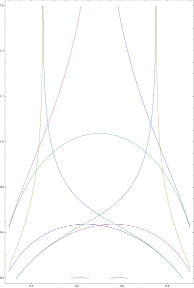
Figure 1. Five degeneracy curves $C_{\pm}$ and $\tilde{C}_{i,j}$ (marked in 5 different colors).

In Section 2, we will review some facts about solutions of Painlevé VI equation. Among them, there are solutions which can be reduced to solve first order differential equations, the so-called Riccati type equations. Riccati type equations were already well studied by Poincare in the 19th century. We could write down the explicit expression for solutions of those Riccati type equations related to certain Painlevé VI equation. In Section 3, we will prove Theorems 1.1-1.3 by applying the theory of Painlevé VI equation established in Section 2.

Acknowledgements The authors thank Chin-Lung Wang very much for providing the file of Figure 1 to us.

2. Riccati type solutions of Painleve VI equation

The well-known Painlevé VI equation with four free parameters $(\alpha,\beta,\gamma,\delta)$ (PVI$(\alpha,\beta,\gamma,\delta)$) is written as

$$\frac{d^{2}\lambda}{dt^{2}}= \frac{1}{2}\left(\frac{1}{\lambda}+\frac{1}{\lambda-1}+\frac{1}{\lambda-t}\right)\left(\frac{d\lambda}{dt}\right)^{2}-\left(\frac{1}{t}+\frac{1}{t-1}+\frac{1}{\lambda-t}\right)\frac{d\lambda}{dt}$$

(2.1) $$+\frac{\lambda(\lambda-1)(\lambda-t)}{t^{2}(t-1)^{2}}\left[\alpha+\beta\frac{t}{\lambda^{2}}+\gamma\frac{t-1}{(\lambda-1)^{2}}+\delta\frac{t(t-1)}{(\lambda-t)^{2}}\right].$$

Due to its connection with many different disciplines in mathematics and physics, PVI (2.1) has been extensively studied in the past several decades. See [9, 10, 11, 12, 15, 16, 18, 21] and references therein.

One of the fundamental properties for PVI (2.1) is the so-called Painlevé property which says that any solution $\lambda(t)$ of (2.1) has neither movable branch points nor movable essential singularities; in other words, for any $t_{0}\in\mathbb{C}\backslash\{0,1\}$, either $\lambda(t)$ is smooth at $t_{0}$ or $\lambda(t)$ has a pole at $t_{0}$. Furthermore, $\lambda(t)$ has at most simple poles in $\mathbb{C}\backslash\{0,1\}$ if $\alpha\not=0$ (cf. [12, Proposition 1.4.1] or [5, Theorem 3.A]).

By the Painlevé property, it is reasonable to lift PVI (2.1) to the covering space $\mathbb{H=}\{\tau|\operatorname{Im}\tau>0\}$ of $\mathbb{C}\backslash\{0,1\}$ by the following transformation:

(2.2) $$t=\frac{e_{3}(\tau)-e_{1}(\tau)}{e_{2}(\tau)-e_{1}(\tau)},\text{ \ }\lambda(t)=\frac{\wp(p(\tau)|\tau)-e_{1}(\tau)}{e_{2}(\tau)-e_{1}(\tau)}.$$

Then $p(\tau)$ satisfies the following elliptic form of PVI (cf. [1, 16, 19]):

(2.3) $$\frac{d^{2}p(\tau)}{d\tau^{2}}=\frac{-1}{4\pi^{2}}\sum_{k=0}^{3}\alpha_{k}\wp^{\prime}\left(\left.p(\tau)+\frac{\omega_{k}}{2}\right|\tau\right),$$

with parameters given by

(2.4) $$\left(\alpha_{0},\alpha_{1},\alpha_{2},\alpha_{3}\right)=\left(\alpha,-\beta,\gamma,\tfrac{1}{2}-\delta\right).$$

The Painlevé property of PVI (2.1) implies that function $\wp(p(\tau)|\tau)$ is a single-valued meromorphic function in $\mathbb{H}$.

Generically, solutions of PVI (2.1) are transcendental (cf. [21]). However, there are classical solutions such as algebraic solutions (cf. [9, 15]) or Riccati solutions (cf. [21]) for PVI with certain parameters. According to [21], when $\alpha_{k}=\tfrac{1}{2}(n_{k}+\tfrac{1}{2})^{2}$ with $n_{k}\in\mathbb{N\cup\{}0\mathbb{\}}$ for all $k$, PVI (2.1) possesses four $1$-parameter families of solutions which satisfy four Riccati type equations. See also [17]. In this paper, we only consider the case $\alpha_{0}=\frac{9}{8}$ and $\alpha_{k}=\frac{1}{8}$ for $k\geq 1$, i.e. PVI$(\tfrac{9}{8},\tfrac{-1}{8},\tfrac{1}{8},\tfrac{3}{8})$. We will prove that the corresponding four Riccati type equations of PVI$(\tfrac{9}{8},\tfrac{-1}{8},\tfrac{1}{8},\tfrac{3}{8})$ are

(2.5) $$P_{0}\left(\tfrac{d}{dt}\lambda^{(0)}(t),\lambda^{(0)}(t),t\right)=0,$$

(2.6) $$\frac{d\lambda^{(1)}}{dt}=\frac{3(\lambda^{(1)})^{2}-2\lambda^{(1)}-t}{2t(t-1)},$$

(2.7) $$\frac{d\lambda^{(2)}}{dt}=\frac{3(\lambda^{(2)})^{2}-4\lambda^{(2)}+t}{2t(t-1)},$$

(2.8) $$\frac{d\lambda^{(3)}}{dt}=\frac{3(\lambda^{(3)})^{2}-2(t+1)\lambda^{(3)}+t}{2t(t-1)},$$

where

$$P_{0}(y,x,t) =8t^{3}(t-1)^{3}y^{3}-4t^{2}(t-1)^{2}(3x^{2}+2(t-2)x-t)y^{2}$$

(2.9) $$-2t(t-1)(x^{2}-2tx+t)(9x^{2}-2(t+4)x+t)y$$

$$+27x^{6}-6(7t+10)x^{5}+(4t^{2}+101t+32)x^{4}$$

$$+4t(2t^{2}-5t-14)x^{3}-3t^{2}(4t-3)x^{2}+2t^{2}(3t+2)x-t^{3}.$$

Remark 2.1.

Notice that equation (2.5) is cubic in $\tfrac{d}{dt}\lambda^{(0)}(t)$ and hence not precisely a Riccati equation. Here we call it a Riccati type equation because it will be obtained from a Riccati equation by applying the Okamoto transformation.

The main result of this section is

Theorem 2.2.

For any $k\in\{0,1,2,3\}$ and $C\in\mathbb{C}\cup\{\infty\}$,

$$\lambda_{C}^{(k)}(t)=\frac{\wp(p_{C}^{(k)}(\tau)|\tau)-e_{1}(\tau)}{e_{2}(\tau)-e_{1}(\tau)}$$

is a solution of the $k$-th Riccati type equation in (2.5)-(2.8), where $\wp(p_{C}^{(k)}(\tau)|\tau)$ are given by:

(2.10) $$\wp(p_{C}^{(0)}(\tau)|\tau)$$

$$= \frac{-4(C\eta_{1}-\eta_{2})^{3}-g_{2}(C\eta_{1}-\eta_{2})(C-\tau)^{2}+2g_{3}(C-\tau)^{3}}{(C-\tau)[12(C\eta_{1}-\eta_{2})^{2}-g_{2}(C-\tau)^{2}]},$$

and

(2.11) $$\wp(p_{C}^{(k)}(\tau)|\tau)=\frac{(\frac{g_{2}}{2}-3e_{k}^{2})(C\eta_{1}-\eta_{2})+\frac{g_{2}}{4}e_{k}(C-\tau)}{3e_{k}(C\eta_{1}-\eta_{2})+(\frac{g_{2}}{2}-3e_{k}^{2})(C-\tau)}$$

for $k\in\{1,2,3\}$.

Furthermore, such $\lambda_{C}^{(k)}(t)$ gives all the Riccati type solutions of PVI$(\frac{9}{8},\frac{-1}{8},\frac{1}{8},\frac{3}{8})$.

We will prove Theorem 2.2 by applying the Okamoto transformation [18] from PVI$(\frac{1}{8},\frac{-1}{8},\frac{1}{8},\frac{3}{8})$ to PVI$(\frac{9}{8},\frac{-1}{8},\frac{1}{8},\frac{3}{8})$. It is well known that any solution $\lambda(t)$ of PVI (2.1) corresponds to a solution $(\lambda(t),\mu(t))$ of a Hamiltonian system (cf. [12]):

(2.12) $$\frac{d\lambda(t)}{dt}=\frac{\partial K(\lambda,\mu,t)}{\partial\mu},\text{ \ }\frac{d\mu(t)}{dt}=-\frac{\partial K(\lambda,\mu,t)}{\partial\lambda},$$

and the Okamoto transformation is a bi-rational transformation concerning solutions of the Hamiltonian systems (2.12) with different PVI parameters. For our case, we note that PVI$(\tfrac{1}{2}(n+\tfrac{1}{2})^{2},\tfrac{-1}{8},\tfrac{1}{8},\tfrac{3}{8})$ is equivalent to the Hamiltonian system (2.12) with $K(\lambda,\mu,t)=K_{n}$ given by

(2.13) $$K_{n}=\frac{1}{t(t-1)}\left\{\begin{array}[c]{l}\lambda(\lambda-1)(\lambda-t)\mu^{2}\\ -\frac{1}{2}(\lambda^{2}-2t\lambda+t)\mu-\frac{n(n+1)}{4}(\lambda-t)\end{array}\right\}.$$

Applying a special case of [5, Lemma 3.3], we know that a solution $(\tilde{\lambda},\tilde{\mu})$ of the Hamiltonian system (2.12)-(2.13) corresponding to PVI$(\frac{1}{8},\frac{-1}{8},\frac{1}{8},\frac{3}{8})$ (i.e. $n=0$) is transformed to a solution $(\lambda,\mu)$ of the Hamiltonian system (2.12)-(2.13) corresponding to PVI$(\frac{9}{8},\frac{-1}{8},\frac{1}{8},\frac{3}{8})$ (i.e. $n=1$) by the following formulas:

(2.14) $$\mu=\tilde{\mu}-\frac{1}{2}\left(\frac{1}{\tilde{\lambda}}+\frac{1}{\tilde{\lambda}-1}+\frac{1}{\tilde{\lambda}-t}\right),$$

(2.15) $$\lambda=\tilde{\lambda}+\frac{1}{\mu}.$$

We recall that for PVI$(\frac{1}{8},\frac{-1}{8},\frac{1}{8},\frac{3}{8})$, the corresponding four Riccati equations are

(2.16) $$\frac{d\tilde{\lambda}^{(0)}}{dt}=-\frac{(\tilde{\lambda}^{(0)})^{2}-2t\tilde{\lambda}^{(0)}+t}{2t(t-1)},\text{ \ \ }\tilde{\mu}^{(0)}\equiv 0,$$

(2.17) $$\frac{d\tilde{\lambda}^{(1)}}{dt}=\frac{(\tilde{\lambda}^{(1)})^{2}-2\tilde{\lambda}^{(1)}+t}{2t(t-1)},\text{ \ \ }\tilde{\mu}^{(1)}\equiv\frac{1}{2\tilde{\lambda}^{(1)}},$$

(2.18) $$\frac{d\tilde{\lambda}^{(2)}}{dt}=\frac{(\tilde{\lambda}^{(2)})^{2}-t}{2t(t-1)},\text{ \ \ }\tilde{\mu}^{(2)}\equiv\frac{1}{2(\tilde{\lambda}^{(2)}-1)},$$

(2.19) $$\frac{d\tilde{\lambda}^{(3)}}{dt}=\frac{(\tilde{\lambda}^{(3)})^{2}+2(t-1)\tilde{\lambda}^{(3)}-t}{2t(t-1)},\text{ \ \ }\tilde{\mu}^{(3)}\equiv\frac{1}{2(\tilde{\lambda}^{(3)}-t)}.$$

In [6], we have completely solved all the equations (2.16)-(2.19).

Theorem 2.A. [6]  For any $k\in\{0,1,2,3\}$ and $C\in\mathbb{C}\cup\{\infty\}$,

$$\tilde{\lambda}_{C}^{(k)}(t)=\frac{\wp(\tilde{p}_{C}^{(k)}(\tau)|\tau)-e_{1}(\tau)}{e_{2}(\tau)-e_{1}(\tau)}$$

is a solution of the $k$-th Riccati equation in (2.16)-(2.19), where $\wp(\tilde{p}_{C}^{(k)}(\tau)|\tau)$ are given by:

(2.20) $$\wp(\tilde{p}_{C}^{(0)}(\tau)|\tau)=\frac{\eta_{2}(\tau)-C\eta_{1}(\tau)}{C-\tau}\text{,}$$

and

(2.21) $$\wp(\tilde{p}_{C}^{(k)}(\tau)|\tau)=\frac{e_{k}(C\eta_{1}(\tau)-\eta_{2}(\tau))+(\frac{g_{2}}{4}-2e_{k}^{2})(C-\tau)}{C\eta_{1}(\tau)-\eta_{2}(\tau)+e_{k}(C-\tau)}$$

for $k\in\{1,2,3\}$. Furthermore, such $\tilde{\lambda}_{C}^{(k)}(t)$ gives all the Riccati type solutions of PVI$(\frac{1}{8},\frac{-1}{8},\frac{1}{8},\frac{3}{8})$.

Formulae (2.20) and (2.21) were first obtained in [11, 20] and later we proved in [6] that they actually give solutions of the four Riccati equations (2.16)-(2.19). Now we are in a position to prove Theorem 2.2.

Proof of Theorem 2.2.

Let $(\tilde{\lambda},\tilde{\mu})$ be any Riccati solution of the Hamiltonian system (2.12) corresponding to PVI$(\frac{1}{8},\frac{-1}{8},\frac{1}{8},\frac{3}{8})$, i.e. $(\tilde{\lambda},\tilde{\mu})$ satisfies one of the four Riccati equations (2.16)-(2.19). Let $(\lambda,\mu)$ be defined by the Okamoto transformation (2.14)-(2.15) via $(\tilde{\lambda},\tilde{\mu})$. Then $(\lambda,\mu)$ is a solution of the Hamiltonian system (2.12) corresponding to PVI$(\frac{9}{8},\frac{-1}{8},\frac{1}{8},\frac{3}{8})$. Applying the Hamiltonian system (2.12)-(2.13) with $n=1$, we obtain

(2.22) $$\lambda^{\prime}(t)=\frac{1}{t(t-1)}\left[2\lambda(\lambda-1)(\lambda-t)\mu-\tfrac{1}{2}(\lambda^{2}-2t\lambda+t)\right],$$

which gives

(2.23) $$\mu=\frac{t(t-1)\lambda^{\prime}+\tfrac{1}{2}(\lambda^{2}-2t\lambda+t)}{2\lambda(\lambda-1)(\lambda-t)}.$$

In the following proof, we omit the superscript $(k)$ and the subscript $C$ for convenience, i.e. write $\tilde{\lambda}_{C}^{(k)}=\tilde{\lambda}$ and so on.

Case 1. $\tilde{p}(\tau)$ satisfies (2.20), i.e. $\tilde{\lambda}(t)$ solves the Riccati equation (2.16).

Then $\tilde{\mu}\equiv 0$, so we see from (2.14)-(2.15) that

$$\lambda=\tilde{\lambda}-\frac{2\tilde{\lambda}(\tilde{\lambda}-1)(\tilde{\lambda}-t)}{\tilde{\lambda}(\tilde{\lambda}-1)+\tilde{\lambda}(\tilde{\lambda}-t)+(\tilde{\lambda}-1)(\tilde{\lambda}-t)}.$$

By this, $t=\frac{e_{3}-e_{1}}{e_{2}-e_{1}}$ and $4\wp^{3}-g_{2}\wp-g_{3}=4(\wp-e_{1})(\wp-e_{2})(\wp-e_{3})$, we easily obtain

(2.24) $$\wp(p(\tau)|\tau)=\frac{4\wp(\tilde{p}(\tau)|\tau)^{3}+g_{2}\wp(\tilde{p}(\tau)|\tau)+2g_{3}}{12\wp(\tilde{p}(\tau)|\tau)^{2}-g_{2}}.$$

Inserting (2.20), i.e $\wp(\tilde{p}(\tau)|\tau)=\frac{\eta_{2}(\tau)-C\eta_{1}(\tau)}{C-\tau}$ into (2.24), we see that $\wp(p(\tau)|\tau)$ satisfies (2.10). To obtain the first order differential equation that $\lambda(t)$ solves, we see from $\tilde{\mu}\equiv 0$ and (2.14)-(2.15) that

(2.25) $$\mu+\frac{1}{2}\left(\frac{1}{\lambda-\frac{1}{\mu}}+\frac{1}{\lambda-\frac{1}{\mu}-1}+\frac{1}{\lambda-\frac{1}{\mu}-t}\right)=0.$$

Inserting (2.23) into (2.25), a straightforward computation gives

$$P_{0}(\lambda^{\prime},\lambda,t)\cdot\left[2t(t-1)\lambda^{\prime}+\lambda^{2}-2t\lambda+t\right]=0.$$

If $2t(t-1)\lambda^{\prime}+\lambda^{2}-2t\lambda+t=0$, then $\lambda(t)$ solves the Riccati equation (2.16) and so satisfies PVI$(\frac{1}{8},\frac{-1}{8},\frac{1}{8},\frac{3}{8})$, clearly a contradiction. Thus $\lambda(t)$ solves the first order algebraic equation (2.5).

Case 2. $\tilde{p}(\tau)$ satisfies (2.21), i.e. $\tilde{\lambda}(t)$ solves the Riccati equation (2.17) if $k=1$, (2.18) if $k=2$ and (2.19) if $k=3$.

Without loss of generality, we may assume $k=1$, since the other two cases $k=2,3$ can be proved in the same way. Then $\tilde{\lambda}(t)$ solves the Riccati equation (2.17) and $\tilde{\mu}\equiv\frac{1}{2\tilde{\lambda}}$. Consequently, (2.14)-(2.15) give

(2.26) $$\lambda=\frac{(1+t)\tilde{\lambda}-2t}{2\tilde{\lambda}-1-t},$$

and then

(2.27) $$\wp(p(\tau)|\tau)=-\frac{e_{1}\wp(\tilde{p}(\tau)|\tau)+2e_{1}^{2}-\frac{g_{2}}{2}}{2\wp(\tilde{p}(\tau)|\tau)+e_{1}},$$

where $t=\frac{e_{3}-e_{1}}{e_{2}-e_{1}}$, $e_{1}+e_{2}+e_{3}=0$ and $-\frac{g_{2}}{4}=e_{2}e_{3}-e_{1}^{2}$ are used. Inserting (2.21) with $k=1$ into (2.27), it is easy to see that $\wp(p(\tau)|\tau)$ satisfies (2.11) with $k=1$. To obtain the first order differential equation that $\lambda(t)$ satisfies, we note from (2.26) that

$$\tilde{\lambda}=\frac{(1+t)\lambda-2t}{2\lambda-1-t}.$$

This, together with (2.15), implies

(2.28) $$\mu=\frac{1}{\lambda-\tilde{\lambda}}=\frac{2\lambda-1-t}{2(\lambda-1)(\lambda-t)}.$$

Inserting (2.28) into (2.22), we see that $\lambda(t)$ solves the Riccati equation (2.6).

Finally, we note that the Okamoto transformation is invertible. Since Theorem 2.A shows that such $\tilde{\lambda}(t)$ gives all the Riccati type solutions of PVI$(\frac{1}{8},\frac{-1}{8},\frac{1}{8},\frac{3}{8})$, we conclude that such $\lambda(t)$ gives all the Riccati type solutions of PVI$(\frac{9}{8},\frac{-1}{8},\frac{1}{8},\frac{3}{8})$. The proof is complete. ∎

Remark that if $C=\infty$, then formulae (2.10)-(2.11) turn to be

$$\wp(p_{\infty}^{(0)}(\tau)|\tau)=\frac{-4\eta_{1}^{3}-g_{2}\eta_{1}+2g_{3}}{12\eta_{1}^{2}-g_{2}},$$

$$\wp(p_{\infty}^{(k)}(\tau)|\tau)=\frac{(\frac{g_{2}}{2}-3e_{k}^{2})\eta_{1}+\frac{g_{2}}{4}e_{k}}{3e_{k}\eta_{1}+\frac{g_{2}}{2}-3e_{k}^{2}},$$

respectively. To apply Theorem 2.2 in Section 3, we conclude this section by proving the following technical lemma.

Lemma 2.3.

Let $C\in\mathbb{C}\cup\{\infty\}$, $k\in\{1,2,3\}$ and $\tau\in\mathbb{H}$.

• If $C\not=\infty$ and

  (2.29) $$(C-\tau)[12(C\eta_{1}-\eta_{2})^{2}-g_{2}(C-\tau)^{2}]=0,$$

  then

  $$-4(C\eta_{1}-\eta_{2})^{3}-g_{2}(C\eta_{1}-\eta_{2})(C-\tau)^{2}+2g_{3}(C-\tau)^{3}\not=0.$$

• If $12\eta_{1}^{2}-g_{2}=0$, then $-4\eta_{1}^{3}-g_{2}\eta_{1}+2g_{3}\not=0$.

• If $C\not=\infty$ and

  (2.30) $$3e_{k}(C\eta_{1}-\eta_{2})+(\tfrac{g_{2}}{2}-3e_{k}^{2})(C-\tau)=0,$$

  then

  $$(\tfrac{g_{2}}{2}-3e_{k}^{2})(C\eta_{1}-\eta_{2})+\tfrac{g_{2}}{4}e_{k}(C-\tau)\not=0.$$

• If $3e_{k}\eta_{1}+\frac{g_{2}}{2}-3e_{k}^{2}=0$, then $(\frac{g_{2}}{2}-3e_{k}^{2})\eta_{1}+\frac{g_{2}}{4}e_{k}\not=0$.

Proof.

In this proof we denote $x=C\eta_{1}-\eta_{2}$ and $y=C-\tau$ for convenience. By the Legendre relation $\tau\eta_{1}-\eta_{2}=2\pi i$ we have $x=2\pi i+\eta_{1}y$, so

(2.31) $$x,y\text{ can not vanish simultaneously.}$$

(i)-(ii). First consider $C\not=\infty$. Suppose that both (2.29) and

(2.32) $$-4x^{3}-g_{2}xy^{2}+2g_{3}y^{3}=0$$

hold. Then (2.31) gives $x\not=0$, $y\not=0$ and so (2.29) implies $x=\pm\sqrt{g_{2}/12}y$. Inserting this into (2.32), we easily obtain $g_{2}^{3}-27g_{3}^{2}=0$, a contradiction. This proves (i). Similarly we can prove (ii).

(iii)-(iv). Fix $k\in\{1,2,3\}$ and let $\{i,j\}=\{1,2,3\}\backslash\{k\}$. By $\tfrac{g_{2}}{4}=e_{k}^{2}-e_{i}e_{j}$ and $e_{i}+e_{j}+e_{k}=0$ we have

$$\det\begin{pmatrix}3e_{k}&\tfrac{g_{2}}{2}-3e_{k}^{2}\\ \tfrac{g_{2}}{2}-3e_{k}^{2}&\tfrac{g_{2}}{4}e_{k}\end{pmatrix} =(2e_{k}^{2}+e_{i}e_{j})(e_{k}^{2}-4e_{i}e_{j})$$

$$=(2e_{i}+e_{j})(e_{i}+2e_{j})(e_{i}-e_{j})^{2}$$

$$=(e_{i}-e_{k})(e_{j}-e_{k})(e_{i}-e_{j})^{2}\not=0.$$

Together with (2.31), we obtain (iii)-(iv). ∎

3. Simple zero property and application

The purpose of this section is to prove Theorems 1.1-1.3. For $C\in\mathbb{C}\cup\{\infty\}$ and $k\in\{1,2,3\}$, we recall functions $f_{k,C}(\tau)$ from $\mathbb{H}$ to $\mathbb{C}\cup\{\infty\}$ defined in Section 1:

(3.1) $$f_{0,C}(\tau):=\left\{\begin{array}[c]{c}12(C\eta_{1}(\tau)-\eta_{2}(\tau))^{2}-g_{2}(\tau)(C-\tau)^{2}\text{ if }C\not=\infty,\\ 12\eta_{1}(\tau)^{2}-g_{2}(\tau)\text{ \ \ \ \ \ if \ \ \ \ \ }C=\infty,\end{array}\right.$$

(3.2) $$f_{k,C}(\tau):=\left\{\begin{array}[c]{l}3e_{k}(\tau)(C\eta_{1}(\tau)-\eta_{2}(\tau))\\ +(\tfrac{g_{2}(\tau)}{2}-3e_{k}(\tau)^{2})(C-\tau)\text{ \ \ if \ \ }C\not=\infty,\\ 3e_{k}(\tau)\eta_{1}(\tau)+\tfrac{g_{2}(\tau)}{2}-3e_{k}(\tau)^{2}\text{ \ \ if \ \ }C=\infty,\end{array}\right.$$

and functions $\phi_{\pm}(\tau)$ and $\phi_{k}(\tau)$ defined in Section 1:

(3.3) $$\phi_{\pm}(\tau):=\tau-\frac{2\pi i}{\eta_{1}(\tau)\pm\sqrt{g_{2}(\tau)/12}},$$

(3.4) $$\phi_{k}(\tau):=\tau-\frac{6\pi ie_{k}(\tau)}{3e_{k}(\tau)\eta_{1}(\tau)+\frac{g_{2}(\tau)}{2}-3e_{k}(\tau)^{2}}=\tau-\frac{6\pi ie_{k}(\tau)}{f_{k,\infty}(\tau)}.$$

Clearly $\phi_{\pm}(\tau)$ have branch points at $\tau\in\mathfrak{S}$, where

$$\mathfrak{S}=\left\{\frac{ae^{\pi i/3}+b}{ce^{\pi i/3}+d}\left|\begin{pmatrix}a&b\\ c&d\end{pmatrix}\in SL(2,\mathbb{Z})\right.\right\},$$

because $g(\tau)=0$ if and only if $\tau\in\mathfrak{S}$. Remark that

(3.5) $$\phi_{\pm}(\tau)=\tau-\frac{2\pi i}{\eta_{1}(\tau)}=\frac{\eta_{2}(\tau)}{\eta_{1}(\tau)}\not\in\mathbb{R\cup\{\infty\}},\text{ \ \ }\forall\tau\in\mathfrak{S.}$$

In fact, for $\tau=\rho:=e^{\pi i/3}$, since $\wp(z|\rho)=\rho^{2}\wp(\rho z|\rho)$ (cf. [13]), we have $\zeta(z|\rho)=\rho\zeta(\rho z|\rho)$, which gives

$$\eta_{1}(\rho)=2\zeta(1/2|\rho)=2\rho\zeta(\rho/2|\rho)=\rho\eta_{2}(\rho),$$

i.e., $\frac{\eta_{2}(\rho)}{\eta_{1}(\rho)}=\frac{1}{\rho}\not\in\mathbb{R\cup\{\infty\}}$. For any other $\tau\in\mathfrak{S}$, $\tau=\frac{a\rho+b}{c\rho+d}$ for some $\begin{pmatrix}a&b\\ c&d\end{pmatrix}\in SL(2,\mathbb{Z})$. Then by (cf. [7, (4.3)])

$$\begin{pmatrix}\eta_{2}(\tau)\\ \eta_{1}(\tau)\end{pmatrix}=(c\rho+d)\begin{pmatrix}a&b\\ c&d\end{pmatrix}\begin{pmatrix}\eta_{2}(\rho)\\ \eta_{1}(\rho)\end{pmatrix},$$

we obtain

$$\frac{\eta_{2}(\tau)}{\eta_{1}(\tau)}=\frac{a\eta_{2}(\rho)+b\eta_{1}(\rho)}{c\eta_{2}(\rho)+d\eta_{1}(\rho)}=\frac{a\frac{1}{\rho}+b}{c\frac{1}{\rho}+d}\not\in\mathbb{R\cup\{\infty\}},$$

so (3.5) holds. As an application of Theorem 2.2, we obtain the following result, which immediately implies Theorems 1.1 and 1.2.

Theorem 3.1.

For $C\in\mathbb{C}\cup\{\infty\}$ and $k\in\{1,2,3\}$, let $f_{0,C}(\tau)$, $f_{k,C}(\tau)$, $\phi_{\pm}(\tau)$ and $\phi_{k}(\tau)$ be defined in (3.1)-(3.4).

• For any $k\in\{0,1,2,3\}$, $f_{k,C}(\tau)$ has only simple zeros in $\mathbb{H}$.

• $\phi_{\pm}^{\prime}(\tau)\not=0$ for any $\tau\in\mathbb{H}\backslash\mathfrak{S}$. In particular, $\phi_{\pm}(\tau)$ has only simple zeros in $\mathbb{H}$ and is locally one-to-one from $\mathbb{H}\backslash\mathfrak{S}$ to $\mathbb{C}\cup\{\infty\}$.

• For $k\in\{1,2,3\}$, $\phi_{k}^{\prime}(\tau)\not=0$ for any $\tau\in\mathbb{H}$. In particular, $\phi_{k}(\tau)$ has only simple zeros in $\mathbb{H}$ and is locally one-to-one from $\mathbb{H}$ to $\mathbb{C}\cup\{\infty\}$.

Proof.

(i) Recalling

$$\lambda_{C}^{(k)}(t)=\frac{\wp(p_{C}^{(k)}(\tau)|\tau)-e_{1}(\tau)}{e_{2}(\tau)-e_{1}(\tau)},\text{ \ }t=t(\tau)=\frac{e_{3}(\tau)-e_{1}(\tau)}{e_{2}(\tau)-e_{1}(\tau)},$$

Theorem 2.2 and Lemma 2.3 imply that for any zero $\tau_{0}\in\mathbb{H}$ of $f_{k,C}(\tau)$, $t(\tau_{0})\in\mathbb{C}\backslash\{0,1\}$ is a pole of the corresponding solution $\lambda_{C}^{(k)}(t)$ to PVI$(\frac{9}{8},\frac{-1}{8}$, $\frac{1}{8},\frac{3}{8})$. Since $t^{\prime}(\tau)\not=0$ for all $\tau\in\mathbb{H}$ and any pole $t_{0}\in\mathbb{C}\backslash\{0,1\}$ of any solution of PVI$(\frac{9}{8},\frac{-1}{8}$, $\frac{1}{8},\frac{3}{8})$ is a simple pole (cf. [12, Proposition 1.4.1] or [5, Theorem 3.A]), the assertion (i) follows readily.

(ii) Consider function $\phi_{+}(\tau)$. Fix any $\tau_{0}\in\mathbb{H}\backslash\mathfrak{S}$, then $g_{2}(\tau_{0})\not=0$. If $\eta_{1}(\tau_{0})+\sqrt{g_{2}(\tau_{0})/12}=0$, then assertion (i) implies that $\tau_{0}$ is a simple zero of $\eta_{1}(\tau)+\sqrt{g_{2}(\tau)/12}$, so $\phi_{+}^{\prime}(\tau_{0})\not=0$. It suffices to consider $\eta_{1}(\tau_{0})+\sqrt{g_{2}(\tau_{0})/12}\not=0$. Then by letting

(3.6) $$C:=\phi_{+}(\tau_{0})=\tau_{0}-\frac{2\pi i}{\eta_{1}(\tau_{0})+\sqrt{g_{2}(\tau_{0})/12}},$$

we see from $\tau\eta_{1}-\eta_{2}=2\pi i$ that $\tau_{0}$ is a zero of

$$\psi(\tau) :=2\pi i+(C-\tau)\left(\eta_{1}(\tau)+\sqrt{g_{2}/12}\right)$$

$$=C\eta_{1}(\tau)-\eta_{2}(\tau)+\sqrt{g_{2}/12}(C-\tau),$$

which implies that $\tau_{0}$ is a zero of

$$f_{0,C}(\tau)=12\left[C\eta_{1}(\tau)-\eta_{2}(\tau)-\sqrt{g_{2}/12}(C-\tau)\right]\psi(\tau).$$

Then (i) gives $\psi^{\prime}(\tau_{0})\not=0$, i.e.,

$$\eta_{1}(\tau_{0})+\sqrt{g_{2}(\tau_{0})/12}+(\tau_{0}-C)\frac{d}{d\tau}\left.\left(\eta_{1}(\tau)+\sqrt{g_{2}/12}\right)\right|_{\tau=\tau_{0}}\not=0.$$

Together with (3.6) and (3.3), we easily obtain $\phi_{+}^{\prime}(\tau_{0})\not=0$. Similarly we can prove $\phi_{-}^{\prime}(\tau)\not=0$ for any $\tau\in\mathbb{H}\backslash\mathfrak{S}$. This together with (3.5) proves (ii).

(iii) Now we consider function $\phi_{k}(\tau)$ defined in (3.4). Fix $k\in\{1,2,3\}$ and any $\tau_{0}\in\mathbb{H}$. If $f_{k,\infty}(\tau_{0})=0$, then it is easy to see that $e_{k}(\tau_{0})\not=0$ and assertion (i) shows that $\tau_{0}$ is a simple zero of $f_{k,\infty}$, so $\phi_{k}^{\prime}(\tau_{0})\not=0$. It suffices to consider $f_{k,\infty}(\tau_{0})\not=0$. Then by letting

(3.7) $$C:=\phi_{k}(\tau_{0})=\tau_{0}-\frac{6\pi ie_{k}(\tau_{0})}{f_{k,\infty}(\tau_{0})},$$

it follows from $\tau\eta_{1}-\eta_{2}=2\pi i$ that $f_{k,C}(\tau_{0})=0$, where $f_{k,C}(\tau)$ is defined in (3.2), i.e.,

$$f_{k,C}(\tau)=6\pi ie_{k}(\tau)+(C-\tau)f_{k,\infty}(\tau).$$

Again (i) gives $f_{k,C}^{\prime}(\tau_{0})\not=0$, i.e.,

$$6\pi ie_{k}^{\prime}(\tau_{0})-f_{k,\infty}(\tau_{0})+(C-\tau_{0})f_{k,\infty}^{\prime}(\tau_{0})\not=0.$$

Together with (3.7) and (3.4), we easily obtain $\phi_{k}^{\prime}(\tau_{0})\not=0$.

This completes the proof. ∎

It is interesting to note that Theorem 3.1 has important applications in the theory of Green functions. Recall the multiple Green function $G_{2}(z_{1},z_{2}|\tau)$ defined by

$$G_{2}(z_{1},z_{2}|\tau):=G(z_{1}-z_{2}|\tau)-2G(z_{1}|\tau)-2G(z_{2}|\tau).$$

It is easy to see that $G_{2}$ has five trivial critical points $\{(\frac{1}{2}\omega_{i},\frac{1}{2}\omega_{j})$ $|$ $i\not=j\}$ and $\{(q_{\pm},-q_{\pm})$ $|$ $\wp(q_{\pm})=\pm\sqrt{g_{2}/12}\}$, see [14] or Appendix A. The function $G_{2}$ has deep connections with the following mean field equation

(3.8) $$\triangle u+e^{u}=16\pi\delta_{0}\text{ \ \ in \ }E_{\tau}.$$

It was proved in [3] that the mean field equation (3.8) has a solution in $E_{\tau}$ if and only if $G_{2}(\cdot\cdot|\tau)$ has a non-trivial critical point. Therefore, it is important to study the degeneracy of $G_{2}$ at trivial critical points. Denote $\{i,j,k\}=\{1,2,3\}$ and note that

$$2e_{i}e_{j}+e_{k}^{2}-3e_{k}\eta_{1}=3e_{k}^{2}-3e_{k}\eta_{1}-\frac{g_{2}}{2}=-f_{k,\infty}(\tau).$$

Recall that the Hessian of $G_{2}$ at these five trivial critical points are expressed by (see [14, Section 5] or Appendix A)

(3.9) $$\det D^{2}G_{2}(\tfrac{1}{2}\omega_{i},\tfrac{1}{2}\omega_{j}|\tau)$$

$$= \frac{4}{(2\pi)^{4}}\left(|2e_{i}e_{j}+e_{k}^{2}-3e_{k}\eta_{1}|^{2}+\frac{2\pi}{\operatorname{Im}\tau}\operatorname{Re}\left(3\bar{e}_{k}(2e_{i}e_{j}+e_{k}^{2}-3e_{k}\eta_{1})\right)\right),$$

(3.10) $$\det D^{2}G_{2}(q_{\pm},-q_{\pm}|\tau)$$

$$= \frac{9}{\pi^{4}}|\wp(q_{\pm})|^{2}\left(|\wp(q_{\pm})+\eta_{1}|^{2}-\frac{2\pi}{\operatorname{Im}\tau}\operatorname{Re}(\wp(q_{\pm})+\eta_{1})\right).$$

Therefore,

$$\det D^{2}G_{2}(\tfrac{1}{2}\omega_{i},\tfrac{1}{2}\omega_{j}|\tau) =\frac{4}{(2\pi)^{4}}\left(|f_{k,\infty}(\tau)|^{2}-\frac{6\pi}{\operatorname{Im}\tau}\operatorname{Re}\left(\bar{e}_{k}f_{k,\infty}(\tau)\right)\right)$$

$$=\frac{4|f_{k,\infty}(\tau)|^{2}}{(2\pi)^{4}\operatorname{Im}\tau}\operatorname{Im}\left(\tau-\frac{6\pi ie_{k}(\tau)}{f_{k,\infty}(\tau)}\right)$$

$$=\frac{4|f_{k,\infty}(\tau)|^{2}}{(2\pi)^{4}\operatorname{Im}\tau}\operatorname{Im}\phi_{k}(\tau),$$

and

$$\det D^{2}G_{2}(q_{\pm},-q_{\pm}|\tau)$$

$$= \frac{9}{\pi^{4}\operatorname{Im}\tau}|\wp(q_{\pm})|^{2}|\wp(q_{\pm})+\eta_{1}|^{2}\operatorname{Im}\left(\tau-\frac{2\pi i}{\wp(q_{\pm})+\eta_{1}}\right)$$

$$= \frac{3|g_{2}(\tau)|}{4\pi^{4}\operatorname{Im}\tau}|\wp(q_{\pm})+\eta_{1}|^{2}\operatorname{Im}\phi_{\pm}(\tau),$$

where $\phi_{\pm}(\tau)$, $\phi_{k}(\tau)$ are precisely those functions defined in (3.3)-(3.4). Thus the local one-to-one of $\phi_{\pm}(\tau)$ and $\phi_{k}(\tau)$ in Theorem 3.1 are important for studying the smoothness of the curve in $\mathbb{H}$ where the corresponding trivial critical point is a degenerate critical point of $G_{2}(\cdot,\cdot|\tau)$. Recall the following sets defined in Section 1:

(3.11) $$C_{i,j}:=\left\{\tau|\det D^{2}G_{2}(\tfrac{1}{2}\omega_{i},\tfrac{1}{2}\omega_{j}|\tau)=0\right\},$$

(3.12) $$C_{\pm}:=\left\{\tau|\det D^{2}G_{2}(q_{\pm},-q_{\pm}|\tau)=0\right\},$$

(3.13) $$\tilde{C}_{\pm} :=\left\{\tau\left||\wp(q_{\pm})+\eta_{1}|^{2}\operatorname{Im}\phi_{\pm}(\tau)=0\right.\right\}$$

$$=\left\{\tau\left||\wp(q_{\pm})+\eta_{1}|^{2}-\tfrac{2\pi}{\operatorname{Im}\tau}\operatorname{Re}(\wp(q_{\pm})+\eta_{1})=0\right.\right\}.$$

Theorem 3.2.

Recall $C_{i,j}$, $C_{\pm}$ and $\tilde{C}_{\pm}$ defined in (3.11)-(3.13).

• For $\{i,j,k\}=\{1,2,3\}$, the curve $C_{i,j}$ is smooth.

• the set $C_{\pm}$ is a disjoint union of $\tilde{C}_{\pm}$ and $\mathfrak{S}=\{\tau|g_{2}(\tau)=0\}$, i.e., $C_{\pm}=\tilde{C}_{\pm}\sqcup\mathfrak{S}$. Furthermore, the curve $\tilde{C}_{\pm}$ is smooth.

Proof.

Write $\tau=a+bi$ with $a,b\in\mathbb{R}$.

(i) Fix $i,j,k$ and denote $H(\tau)=\det D^{2}G_{2}(\tfrac{1}{2}\omega_{i},\tfrac{1}{2}\omega_{j}|\tau)$. Recall

$$H(\tau)=\frac{4}{(2\pi)^{4}}\left(|f_{k,\infty}(\tau)|^{2}-\frac{6\pi}{b}\operatorname{Re}\left(\bar{e}_{k}f_{k,\infty}(\tau)\right)\right).$$

For $\tau\in C_{i,j}$ such that $f_{k,\infty}(\tau)=0$, it follows from the expression of $f_{k,\infty}=3e_{k}\eta_{1}+\frac{g_{2}}{2}-3e_{k}^{2}$ that $e_{k}(\tau)\not=0$. Furthermore, Theorem 3.1 says $f_{k,\infty}^{\prime}(\tau)\not=0$, so

$$\bar{e}_{k}(\tau)f_{k,\infty}^{\prime}(\tau)= \left(\operatorname{Re}e_{k}\operatorname{Re}f_{k,\infty}^{\prime}+\operatorname{Im}e_{k}\operatorname{Im}f_{k,\infty}^{\prime}\right)(\tau)$$

$$-i\left(\operatorname{Im}e_{k}\operatorname{Re}f_{k,\infty}^{\prime}-\operatorname{Re}e_{k}\operatorname{Im}f_{k,\infty}^{\prime}\right)(\tau)\not=0.$$

Since

$$\frac{\partial H(\tau)}{\partial a}=-\frac{24\pi}{(2\pi)^{4}b}\left(\operatorname{Re}e_{k}\operatorname{Re}f_{k,\infty}^{\prime}+\operatorname{Im}e_{k}\operatorname{Im}f_{k,\infty}^{\prime}\right)(\tau),$$

$$\frac{\partial H(\tau)}{\partial b}=-\frac{24\pi}{(2\pi)^{4}b}\left(\operatorname{Im}e_{k}\operatorname{Re}f_{k,\infty}^{\prime}-\operatorname{Re}e_{k}\operatorname{Im}f_{k,\infty}^{\prime}\right)(\tau),$$

we obtain $\nabla H(\tau)\not=0$, namely $C_{i,j}$ is smooth near such $\tau$.

For $\tau\in C_{i,j}$ such that $f_{k,\infty}(\tau)\not=0$, we see from

$$H(\tau)=\frac{4|f_{k,\infty}(\tau)|^{2}}{(2\pi)^{4}b}\operatorname{Im}\phi_{k}(\tau)$$

that $C_{i,j}$ is defined by $\operatorname{Im}\phi_{k}=0$ near such $\tau$. Since Theorem 3.1 says $\phi_{k}^{\prime}(\tau)\not=0$ and

$$\frac{\partial\operatorname{Im}\phi_{k}}{\partial a}=\operatorname{Im}\phi_{k}^{\prime},\text{ \ \ }\frac{\partial\operatorname{Im}\phi_{k}}{\partial b}=\operatorname{Re}\phi_{k}^{\prime},$$

we conclude that $C_{i,j}$ is also smooth near such $\tau$. This proves (i).

(ii) We consider the set $C_{+}$. Denote $\varphi(\tau)=\wp(q_{+})+\eta_{1}$ and

(3.14) $$H_{+}(\tau)=|\varphi(\tau)|^{2}-\frac{2\pi}{b}\operatorname{Re}\varphi(\tau)=\frac{1}{b}|\varphi(\tau)|^{2}\operatorname{Im}\phi_{+}(\tau).$$

Recalling $\wp(q_{+})=\sqrt{g_{2}/12}$, we have

$$\det D^{2}G_{2}(q_{+},-q_{+}|\tau)=\frac{3|g_{2}(\tau)|}{4\pi^{4}}H_{+}(\tau),$$

which gives $C_{+}=\tilde{C}_{+}\cup\mathfrak{S}$. If $\tau\in\mathfrak{S}$, i.e. $g_{2}(\tau)=0$, then (3.5) shows $\operatorname{Im}\phi_{+}(\tau)\not=0$ and $\varphi(\tau)=\eta_{1}(\tau)\not=0$, which implies $\tau\not\in\tilde{C}_{+}$. Thus $\tilde{C}_{+}\cap\mathfrak{S}=\emptyset$, i.e. $C_{+}=\tilde{C}_{+}\sqcup\mathfrak{S}$.

It suffices to prove that the curve $\tilde{C}_{+}$ is smooth. For those $\tau\in\tilde{C}_{+}$ such that $\varphi(\tau)=0$, Theorem 3.1-(i) (use $f_{0,\infty}=12\eta_{1}^{2}-g_{2}$ and $g_{2}(\tau)\not=0$) implies $\varphi^{\prime}(\tau)\not=0$. Since

$$\frac{\partial H_{+}(\tau)}{\partial a}=-\frac{2\pi}{b}\operatorname{Re}\varphi^{\prime}(\tau),\text{ \ }\frac{\partial H_{+}(\tau)}{\partial b}=\frac{2\pi}{b}\operatorname{Im}\varphi^{\prime}(\tau),$$

we obtain $\nabla H_{+}(\tau)\not=0$, namely $\tilde{C}_{+}$ is smooth near such $\tau$.

For those $\tau\in\tilde{C}_{+}$ such that $\varphi(\tau)\not=0$, we see from (3.14) that $\tilde{C}_{+}$ is defined by $\operatorname{Im}\phi_{+}=0$ near such $\tau$. Since Theorem 3.1 says $\phi_{+}^{\prime}(\tau)\not=0$ and

$$\frac{\partial\operatorname{Im}\phi_{+}}{\partial a}=\operatorname{Im}\phi_{+}^{\prime},\text{ \ \ }\frac{\partial\operatorname{Im}\phi_{+}}{\partial b}=\operatorname{Re}\phi_{+}^{\prime},$$

we conclude that $\tilde{C}_{+}$ is also smooth near such $\tau$. The proof of $C_{-}$ is similar.

The proof is complete. ∎

Appendix A Trivial critical points of Green function $G_{2}$

In this appendix, we prove that $G_{2}$ has five trivial critical points $\{(\frac{1}{2}\omega_{i},\frac{1}{2}\omega_{j})$ $|$ $i\not=j\}$ and $\{(q_{\pm},-q_{\pm})$ $|$ $\wp(q_{\pm})=\pm\sqrt{g_{2}/12}\}$ and compute the Hessian. A critical point $(a_{1},a_{2})$ of $G_{2}$ satisfies

$$2\nabla G(a_{1}|\tau)=\nabla G(a_{1}-a_{2}|\tau),\text{ \ }2\nabla G(a_{2}|\tau)=\nabla G(a_{2}-a_{1}|\tau),$$

which is equivalent to

(A.1) $$\nabla G(a_{1}|\tau)+\nabla G(a_{2}|\tau)=0,\text{ \ }2\nabla G(a_{1}|\tau)-\nabla G(a_{1}-a_{2}|\tau)=0.$$

Proposition A.1.

Green function $G_{2}(z_{1},z_{2}|\tau)$ has precisely five trivial critical points $\{(\frac{1}{2}\omega_{i},\frac{1}{2}\omega_{j})$ $|$ $i\not=j\}$ and $\{(q_{\pm},-q_{\pm})$ $|$ $\wp(q_{\pm})=\pm\sqrt{g_{2}/12}\}$.

Proof.

Let $(a_{1},a_{2})$ be a trivial critical point, i.e.

$$\{a_{1},a_{2}\}=\{-a_{1},-a_{2}\}\text{ \ in \ }E_{\tau}\text{.}$$

If $a_{1}=-a_{1}$ and $a_{2}=-a_{2}$ in $E_{\tau}$, then $a_{k}$ are both half periods, i.e. $(a_{1},a_{2})\in\{(\frac{1}{2}\omega_{i},\frac{1}{2}\omega_{j})$ $|$ $i\not=j\}$. It suffices to consider the case $a_{1}=-a_{2}$ in $E_{\tau}$. Recall from [13] that

(A.2) $$-4\pi G_{z}(z|\tau)=\zeta(z|\tau)-r\eta_{1}(\tau)-s\eta_{2}(\tau),$$

where $z=r+s\tau$ with $r,s\in\mathbb{R}$. Therefore, the second equation in (A.1) becomes

$$2\zeta(a_{1}|\tau)-\zeta(2a_{1}|\tau)=0.$$

Together with the addition formula $2\zeta(a_{1}|\tau)-\zeta(2a_{1}|\tau)=\frac{-\wp^{\prime\prime}(a_{1}|\tau)}{2\wp^{\prime}(a_{1}|\tau)}$, we obtain

$$6\wp(a_{1}|\tau)^{2}-g_{2}/2=\wp^{\prime\prime}(a_{1}|\tau)=0,$$

i.e. $\wp(a_{1}|\tau)=\pm\sqrt{g_{2}/12}$. The proof is complete. ∎

Now we compute the Hessian of $G_{2}$ at these five trivial critical points.

Proposition A.2.

Let $\{i,j,k\}=\{1,2,3\}$. Then

(A.3) $$\det D^{2}G_{2}(\tfrac{1}{2}\omega_{i},\tfrac{1}{2}\omega_{j}|\tau)$$

$$= \frac{4}{(2\pi)^{4}}\left(|2e_{i}e_{j}+e_{k}^{2}-3e_{k}\eta_{1}|^{2}+\frac{2\pi}{b}\operatorname{Re}\left(3\bar{e}_{k}(2e_{i}e_{j}+e_{k}^{2}-3e_{k}\eta_{1})\right)\right).$$

$$\det D^{2}G_{2}(q_{\pm},-q_{\pm}|\tau)$$

$$=\frac{9}{\pi^{4}}|\wp(q_{\pm})|^{2}\left(|\wp(q_{\pm})+\eta_{1}|^{2}-\frac{2\pi}{\operatorname{Im}\tau}\operatorname{Re}(\wp(q_{\pm})+\eta_{1})\right).$$

Proof.

The following argument is borrowed from [14, Section 5]. First we consider $p=(\frac{1}{2}\omega_{i},\frac{1}{2}\omega_{j})$ where $\{i,j,k\}=\{1,2,3\}$. Notice that $\wp(\frac{1}{2}\omega_{i}-\frac{1}{2}\omega_{j})=\wp(\frac{1}{2}\omega_{k})=e_{k}$. For simplicity we write

$$\tau=a+bi\text{ and }-(e_{k}+\eta_{1})=u_{k}+v_{k}i,$$

and similarly for the indices $i$, $j$, where $a,b,u_{k},v_{k}$ are all real. Then by (A.2), a straightforward computation gives

$$D^{2}G_{2}(p)=\frac{1}{2\pi}\begin{pmatrix}2u_{i}-u_{k}&v_{k}-2v_{i}&u_{k}&-v_{k}\\ v_{k}-2v_{i}&u_{k}-2u_{i}-\frac{2\pi}{b}&-v_{k}&-u_{k}-\frac{2\pi}{b}\\ u_{k}&-v_{k}&2u_{j}-u_{k}&v_{k}-2v_{j}\\ -v_{k}&-u_{k}-\frac{2\pi}{b}&v_{k}-2v_{j}&u_{k}-2u_{j}-\frac{2\pi}{b}\end{pmatrix}.$$

A lengthy yet straightforward calculation shows (A.3). The details will be omit here. We only note that when $\tau\in i\mathbb{R}^{+}$, all $e_{i}$’s and $\eta_{1}$ are real numbers. Thus all the imaginary parts vanish: $v_{1}=v_{2}=v_{3}=0$. In this case (A.3) can be verified easily.

Next we consider $p=(q,-q)$ with $q\in\{q_{+},q_{-}\}$. Let $\mu=\wp(q)=u+iv$ with $u,v$ real. Since $\wp^{\prime\prime}(q)=0$, we have $\wp(2q)=-2\wp(q)=-2\mu$ by the addition formula. Denote $\eta_{1}=s+ti$ with $s,t$ real. Then we have

$$D^{2}G_{2}(p)=\frac{1}{2\pi}\begin{pmatrix}-4u-s&4v+t&2u-s&-2v+t\\ 4v+t&4u+s-\frac{2\pi}{b}&-2v+t&-2u+s-\frac{2\pi}{b}\\ 2u-s&-2v+t&-4u-s&4v+t\\ -2v+t&-2u+s-\frac{2\pi}{b}&4v+t&4u+s-\frac{2\pi}{b}\end{pmatrix}.$$

A straightforward calculation easier than the previous case shows that

$$\det D^{2}G_{2}(p) =\frac{144}{(2\pi)^{4}}(u^{2}+v^{2})\left((u+s)^{2}+(v+t)^{2}-\frac{2\pi}{b}(u+s)\right)$$

$$=\frac{9}{\pi^{4}}|\wp(q)|^{2}\left(|\wp(q)+\eta_{1}|^{2}-\frac{2\pi}{\operatorname{Im}\tau}\operatorname{Re}(\wp(q)+\eta_{1})\right).$$

The proof is complete. ∎

Appendix B Derivative with respect to $\tau$

In this appendix, as mentioned in Section 1, we prove the simple zero property of $F_{k}(\tau)$ and $f_{k,\infty}(\tau)$ by taking derivative directly. Then we explain why this approach can not work for $f_{k,C}(\tau)$ with $C\not=\infty$.

We need to use the following formulas (cf. [2] or [4, Lemma 2.3]):

$$\frac{\partial}{\partial\tau}\wp(z|\tau)=\frac{-i}{4\pi}\left[\begin{array}[c]{l}2\left(\zeta(z|\tau)-z\eta_{1}(\tau)\right)\wp^{\prime}(z|\tau)\\ +4\left(\wp(z|\tau)-\eta_{1}\right)\wp(z|\tau)-\frac{2}{3}g_{2}(\tau)\end{array}\right],$$

(B.1) $$\eta_{1}^{\prime}\left(\tau\right)=\frac{i}{4\pi}\left[2\eta_{1}^{2}-\frac{1}{6}g_{2}(\tau)\right].$$

From here, we immediately obtain

(B.2) $$e_{k}^{\prime}(\tau)=\frac{-i}{4\pi}\left[4\left(e_{k}-\eta_{1}\right)e_{k}-\frac{2}{3}g_{2}(\tau)\right],\text{ \ }k\in\{1,2,3\}.$$

By $g_{2}=2(e_{1}^{2}+e_{2}^{2}+e_{3}^{2})$, $e_{1}+e_{2}+e_{3}=0$ and $g_{3}=4e_{1}e_{2}e_{3}=\frac{4}{3}(e_{1}^{3}+e_{2}^{3}+e_{3}^{3})$, we easily derive from (B.2) that

(B.3) $$g_{2}^{\prime}(\tau)=\frac{-i}{\pi}[3g_{3}(\tau)-2\eta_{1}(\tau)g_{2}(\tau)],$$

$$g_{3}^{\prime}(\tau)=\frac{-i}{\pi}[-3g_{3}(\tau)\eta_{1}(\tau)+\tfrac{1}{6}g_{2}(\tau)^{2}].$$

Proposition B.1.

For $k\in\{1,2,3\}$, $F_{k}(\tau)=\eta_{1}(\tau)+e_{k}(\tau)$ satisfies the simple zero property.

Proof.

Assume $F_{k}(\tau)=0$ for some $\tau$. Then $\eta_{1}(\tau)=-e_{k}(\tau)$ and so (B.1)-(B.2) give

$$F_{k}^{\prime}(\tau) =\frac{i}{4\pi}\left[2\eta_{1}^{2}-4\left(e_{k}-\eta_{1}\right)e_{k}+\frac{1}{2}g_{2}\right]$$

$$=\frac{i}{4\pi}\left[\frac{1}{2}g_{2}-6e_{k}^{2}\right]=\frac{-i}{4\pi}\wp^{\prime\prime}(\tfrac{\omega_{k}}{2}|\tau)\not=0.$$

This completes the proof. ∎

Now we consider $f_{k,\infty}(\tau)$ defined in (1.2)-(1.3).

Proposition B.2.

For $k\in\{0,1,2,3\}$, $f_{k,\infty}(\tau)$ satisfies the simple zero property.

Proof.

Recall

$$f_{0,\infty}(\tau)=12\eta_{1}(\tau)^{2}-g_{2}(\tau).$$

Assume $f_{0,\infty}(\tau)=0$ for some $\tau$. Then (B.1) implies $\eta_{1}^{\prime}\left(\tau\right)=0$, so

$$f_{0,\infty}^{\prime}(\tau)=-g_{2}^{\prime}(\tau)=\frac{i}{\pi}[3g_{3}(\tau)-2\eta_{1}(\tau)g_{2}(\tau)].$$

If $f_{0,\infty}^{\prime}(\tau)=0$, then $3g_{3}=2\eta_{1}g_{2}$, i.e. $27g_{3}^{2}=12\eta_{1}^{2}g_{2}^{2}=g_{2}^{3}$, which is a contradiction. Therefore, $f_{0,\infty}^{\prime}(\tau)\not=0$.

For $k\in\{1,2,3\}$,

$$f_{k,\infty}(\tau)=3e_{k}(\tau)\eta_{1}(\tau)+\tfrac{g_{2}(\tau)}{2}-3e_{k}(\tau)^{2}.$$

By (B.1)-(B.3), a direct computation gives

(B.4) $$f_{k,\infty}^{\prime}(\tau)=\frac{i}{4\pi}\left[24e_{k}^{3}-6\eta_{1}(6e_{k}^{2}-3\eta_{1}e_{k}-g_{2})-\frac{9}{2}e_{k}g_{2}-6g_{3}\right].$$

Let $\{i,j\}=\{1,2,3\}\backslash\{k\}$ and denote $a=e_{k}^{2}$, $b=-e_{i}e_{j}$. Then we easily see from $e_{i}+e_{j}+e_{k}=0$ that

(B.5) $$g_{2}=4(a+b),\text{ \ }g_{3}e_{k}=-4ab,$$

$$a+4b=(e_{i}-e_{j})^{2}\not=0,$$

$$2a-b=(e_{k}-e_{i})(e_{k}-e_{j})\not=0.$$

Assume $f_{k,\infty}(\tau)=0$ for some $\tau$. Then

(B.6) $$3e_{k}\eta_{1}=3e_{k}^{2}-\tfrac{g_{2}}{2}=a-2b.$$

Inserting (B.5) and (B.6) into (B.4), we obtain

$$e_{k}f_{k,\infty}^{\prime}(\tau) =\frac{i}{4\pi}\left[24e_{k}^{4}-2(3e_{k}^{2}-\tfrac{g_{2}}{2})^{2}-\frac{9}{2}e_{k}^{2}g_{2}-6e_{k}g_{3}\right]$$

$$=\frac{i}{4\pi}\left[24a^{2}-2(a-2b)^{2}-18a(a+b)+24ab\right]$$

$$=\frac{i}{2\pi}(2a-b)(a+4b)\not=0,$$

i.e. $f_{k,\infty}^{\prime}(\tau)\not=0$. The proof is complete. ∎

Finally, we explain why the above approach can not work for $f_{k,C}(\tau)$ with $C\not=\infty$. We take $f_{0,C}(\tau)$ for example. By $\eta_{2}=\tau\eta_{1}(\tau)-2\pi i$, we have

(B.7) $$f_{0,C}(\tau)=12[(C-\tau)\eta_{1}(\tau)+2\pi i]^{2}-g_{2}(\tau)(C-\tau)^{2}.$$

Then

(B.8) $$f_{0,C}^{\prime}(\tau) =24[(C-\tau)\eta_{1}(\tau)+2\pi i][(C-\tau)\eta_{1}^{\prime}(\tau)-\eta_{1}(\tau)]$$

$$-g_{2}^{\prime}(\tau)(C-\tau)^{2}+2g_{2}(\tau)(C-\tau).$$

For function $f(\tau)=F_{k}(\tau)$ or $f_{k,\infty}(\tau)$, the key step in the proof of Propositions B.1 and B.2 is: By $f(\tau)=0$ we can eliminate the term $\eta_{1}$ in the expression of $f^{\prime}(\tau)$ such that $f^{\prime}(\tau)$ turns out to be a function of $e_{1},e_{2},e_{3}$ only. Then we can use the property $e_{1}\not=e_{2}\not=e_{3}\not=e_{1}$ to prove $f^{\prime}(\tau)\not=0$.

However, for function $f_{0,C}(\tau)$ with $C\not=\infty$, (B.8), (B.1) and (B.3) show that there are both terms $\eta_{1}$ and $C-\tau$ in the expression of $f_{0,C}^{\prime}(\tau)$. By using $f_{0,C}(\tau)=0$, we can not eliminate both $\eta_{1}$ and $C-\tau$ simultaneously in the expression of $f_{0,C}^{\prime}(\tau)$, namely we can not express $f_{0,C}^{\prime}(\tau)$ only in terms of $e_{1},e_{2},e_{3}$. Therefore, it seems impossible for us to prove $f_{0,C}^{\prime}(\tau)\not=0$ from its expression.

References

[1] M. V. Babich and L. A. Bordag; The elliptic
form of the sixth Painlevé equation. Preprint NT Z25/1997, Leipzig
(1997).
[2]Y. V. Brezhnev; Non-canonical extension of -functions
and modular integrability of -constants. Proc. Roy. Soc. Edinburgh
Sect. A 143 (2013), no. 4, 689–738.
[3] C.L. Chai, C.S. Lin and C.L. Wang; Mean field
equations, Hyperelliptic curves, and Modular forms: I. Cambridge Journal of
Mathematics, 3 (2015), 127-274.
[4]Z. Chen, T.J. Kuo and C.S. Lin; Hamiltonian
system for the elliptic form of Painlevé VI equation. J. Math. Pures
Appl. 106 (2016), 546-581.
[5]Z. Chen, T.J. Kuo and C.S. Lin; Painlevé VI
equation, modular forms and application. preprint, 2016.
[6]Z. Chen, T.J. Kuo and C.S. Lin; Smoothness of real
solutions of Painlevé VI equation with parameter . preprint, 2016.
[7]Z. Chen, T.J. Kuo, C.S. Lin and C.L. Wang; Green
function, Painlevé VI equation and Eisenstein series of weight one. J.
Differ. Geom. to appear, 2016. http://www. math.ntu.edu.tw/dragon/works.htm
[8]S. Dahmen; Counting integral Lamé equations by
means of dessins d’enfants. Trans. Amer. Math. Soc. 359 (2007), 909–922.
[9] B. Dubrovin and M. Mazzocco; Monodromy
of certain Painlevé-VI transcendents and reflection groups. Invent. Math.
141 (2000), 55-147.
[10] V. Gromak, I. Laine and S. Shimomura; Painlevé
differential equations in the complex plane. de Gruyter Studies in
Mathematics 28, Berlin. New York 2002.
[11] N.J. Hitchin; Twistor spaces, Einstein metrics and
isomonodromic deformations. J. Differ. Geom. 42 (1995), no.1,
30-112.
[12] K. Iwasaki, H. Kimura, S. Shimomura and M. Yoshida;
From Gauss to Painlevé: A Modern Theory of Special Functions.
Springer vol. E16, 1991.
[13] C.S. Lin and C.L. Wang; Elliptic functions, Green
functions and the mean field equations on tori. Annals of Math. 172
(2010), no.2, 911-954.
[14] C.S. Lin and C.L. Wang; Mean field equations,
Hyperelliptic curves, and Modular forms: II. arXiv:1502.03295v2 [math. AP]
2015.
[15] O. Lisovyy and Y. Tykhyy; Algebraic
solutions of the sixth Painlevé equation. J. Geom. Phys. 85
(2014), 124-163.
[16] Y. Manin; Sixth Painlevé quation, universal
elliptic curve, and mirror of . Amer. Math. Soc. Transl. (2),
186 (1998), 131–151.
[17]M. Mazzocco; Picard and Chazy solutions to the
Painlevé VI equation. Math. Ann. 321 (2001), 157–195.
[18] K. Okamoto; Studies on the Painlevé
equations. I. Sixth Painlevé equation . Ann. Mat. Pura Appl.
146 (1986), 337-381.
[19] P. Painlevé; Sur les équations
différentialles du second ordre à points critiques fixes. C. R.
Acad. Sic. Paris Sér. I 143 (1906), 1111-1117.
[20]K. Takemura; The Hermite-Krichever Ansatz for
Fuchsian equations with applications to the sixth Painlevé equation and to
finite gap potentials. Math. Z. 263 (2009), 149-194.
[21]H. Watanabe; Birational canonical transformations
and classical solutions of the sixth Painlevé equation. Ann. Scuola Norm.
Sup. Pisa Cl. Sci. (4), 27 (1998), 379-425.