Accelerated and Inexact Soft-Impute for Large-Scale Matrix and Tensor Completion

Abstract

Matrix and tensor completion aim to recover a low-rank matrix / tensor from limited observations and have been commonly used in applications such as recommender systems and multi-relational data mining. A state-of-the-art matrix completion algorithm is Soft-Impute, which exploits the special “sparse plus low-rank” structure of the matrix iterates to allow efficient SVD in each iteration. Though Soft-Impute is a proximal algorithm, it is generally believed that acceleration destroys the special structure and is thus not useful. In this paper, we show that Soft-Impute can indeed be accelerated without comprising this structure. To further reduce the iteration time complexity, we propose an approximate singular value thresholding scheme based on the power method. Theoretical analysis shows that the proposed algorithm still enjoys the fast $O(1/T^{2})$ convergence rate of accelerated proximal algorithms. We also extend the proposed algorithm to tensor completion with the scaled latent nuclear norm regularizer. We show that a similar “sparse plus low-rank” structure also exists, leading to low iteration complexity and fast $O(1/T^{2})$ convergence rate. Besides, the proposed algorithm can be further extended to nonconvex low-rank regularizers, which have better empirical performance than the convex nuclear norm regularizer. Extensive experiments demonstrate that the proposed algorithm is much faster than Soft-Impute and other state-of-the-art matrix and tensor completion algorithms.

1 Introduction

Matrices are common place in data mining applications. For example, in recommender systems, the ratings data can be represented as a sparsely observed user-item matrix [1]. In social networks, user interactions can be modeled by an adjacency matrix [2, 3]. Matrices also appear in applications such as image processing [4, 5, 6], question answering [7] and large scale classification [8].

Due to limited feedback from users, these matrices are usually not fully observed. For example, users may only give opinions on very few items in a recommender system. As the rows/columns are usually related to each other, the low-rank matrix assumption is particularly useful to capture such relatedness, and low-rank matrix completion has become a powerful tool to predict missing values in these matrices. Sound recovery guarantee [9] and good empirical performance [1] have been obtained.

However, directly minimizing the matrix rank is NP-hard [9]. To alleviate this problem, the nuclear norm (which is the sum of singular values) is often used instead. It is known that the nuclear norm is the tightest convex lower bound of the rank [9]. Specifically, consider an $m\times n$ matrix $O$ (without loss of generality, we assume that $m\geq n$), with positions of the observed entries indicated by $\Omega\in\{0,1\}^{m\times n}$, where $\Omega_{ij}=1$ if $O_{ij}$ is observed, and 0 otherwise. The matrix completion tries to find a low-rank matrix $X$ by solving following optimization problem:

$$\min_{X}\frac{1}{2}\|P_{\Omega}(X-O)\|_{F}^{2}+\lambda\|X\|_{*},$$ (1)

where $[P_{\Omega}(A)]_{ij}=A_{ij}$ if $\Omega_{ij}=1$, and 0 otherwise; and $\|\cdot\|_{*}$ is the nuclear norm. Though the nuclear norm is only a surrogate of the matrix rank, there are theoretical guarantees that the underlying matrix can be exactly recovered [9].

Computationally, though the nuclear norm is nonsmooth, problem (1) can be solved by various optimization tools. An early attempt is based on reformulating (1) as a semidefinite program (SDP) [9]. However, SDP solvers have large time and space complexities, and are only suitable for small data sets. For large-scale matrix completion, singular value thresholding (SVT) algorithm [10] pioneered the use of first-order methods . However, a singular value decomposition (SVD) is required in each SVT iteration. This takes $O(mn^{2})$ time and can be computationally expensive. In [11], this is reduced to a partial SVD by computing only the leading singular values/vectors using PROPACK (a variant of the Lanczos algorithm) [12]. Another major breakthrough is made by the Soft-Impute algorithm [13], which utilizes a special “sparse plus low-rank” structure associated with the SVT to efficiently compute the SVD. Empirically, this allows Soft-Impute to perform matrix completion on the entire Netflix data set. The SVT algorithm can also be viewed as a proximal algorithm [14]. Hence, it converges with a $O(1/T)$ rate, where $T$ is the number of iterations [15]. Later, this is further “accelerated”, and the convergence rate is improved to $O(1/T^{2})$ [16, 11]. However, Tibshirani [14] suggested that this is not useful, as the special “sparse plus low-rank” structure crucial to the efficiency of Soft-Impute no longer exist. In other words, the gain in convergence rate is more than compensated by the increase in iteration time complexity.

In this paper, we show that accelerating Soft-Impute is indeed possible while still preserving the “sparse plus low-rank” structure. To further reduce the iteration time complexity, instead of computing SVT exactly using PROPACK [11, 13], we propose an approximate SVT scheme based on the power method [17]. Though the SVT obtained in each iteration is only approximate, we show that convergence can still be as fast as performing exact SVT. Hence, the resultant algorithm has low iteration complexity and fast $O(1/T^{2})$ convergence rate. To further boost performance, we extend the post-processing procedure in [13] to any smooth convex loss function. The proposed algorithm is also extended for nonconvex low-rank regularizers, such as the truncated nuclear norm [18] and log-sum-penalty [9]. which can give better Empirically, these nonconvex low-rank regularizers have better performance than the convex nuclear norm regularizer.

Besides matrices, tensors have also been commonly used to describe the linear and multilinear relationships in the data [19, 20, 21, 4]. Analogous to matrix completion, tensor completion can also be solved by convex optimization algorithms. However, multiple expensive SVDs on large dense matrices are required [4, 20]. To alleviate this problem, we demonstrate that a similar “sparse plus low-rank” structure also exists when the scaled latent nuclear norm [20, 22] is used as the regularizer. We extend the proposed matrix-based algorithm to this tensor scenario. The resulting algorithm has low iteration cost and fast $O(1/T^{2})$ convergence rate. Experiments on matrix/tensor completion problems with both synthetic and real-world data sets show that the proposed algorithm outperforms state-of-the-art algorithms.

Preliminary results of this paper have been reported in a shorter conference version [23]. While only the square loss is used in [23], here we consider more general smooth convex loss functions. Moreover, we extend the proposed algorithm to tensor completion and nonconvex low-rank regularization. Besides, post-processing is proposed to boost the recovery performance for matrix/tensor completion with nuclear norm regularization. All proofs can be found in Appendix A.

Notation. In the sequel, the transpose of vector/ matrix is denoted by the superscript $\cdot^{\top}$, and tensors are denoted by boldface Euler. For a vector $x$, $\|x\|_{1}=\sum_{i}|x_{i}|$ is its $\ell_{1}$-norm, and $\|x\|=\sqrt{\sum_{i}x_{i}^{2}}$ its $\ell_{2}$-norm. For a matrix $X$, $\sigma_{1}(X)\geq\sigma_{2}(X)\geq\dots\sigma_{m}(X)$ are its singular values, $\,\text{tr}(X)=\sum_{i}X_{ii}$ is its trace, $\|X\|_{1}=\sum_{i,j}|X_{ij}|$, $\|X\|_{\infty}$ is its maximum singular value, and $\|X\|_{F}=\,\text{tr}(X^{\top}X)$ the Frobenius norm, $\|X\|_{*}=\sum_{i}\sigma_{i}(X)$ the nuclear norm, and $\text{span}(X)$ is the column span of $X$. Moreover, $I$ denotes the identity matrix.

For tensors, we follow the notations in [19]. For a $D$-order tensor ${{\boldsymbol{\mathbf{\mathscr{{X}}}}}}\in\mathbb{R}^{I_{1}\times I_{2}\times\cdots\times I_{D}}$, its $(i_{1},i_{2},\dots,i_{D})$th entry is $x_{i_{1}i_{2}\dots i_{D}}$. Let $I_{D\backslash d}=\prod_{j=1,j\neq d}^{D}I_{j}$, the mode-$d$ matricizations ${{\boldsymbol{\mathbf{\mathscr{{X}}}}}}_{\left\langle d\right\rangle}$ of ${{\boldsymbol{\mathbf{\mathscr{{X}}}}}}$ is a $I_{d}\times I_{D\backslash d}$ matrix with $({{\boldsymbol{\mathbf{\mathscr{{X}}}}}}_{\left\langle d\right\rangle})_{i_{d}j}=x_{i_{1}i_{2}\cdots i_{D}}$, and $j=1+\sum_{l=1,l\neq d}^{D}(i_{l}-1)\prod_{m=1,m\neq d}^{l-1}I_{m}$. Given a matrix $A$, its mode-$d$ tensorization $A^{\left\langle d\right\rangle}$ is a tensor ${{\boldsymbol{\mathbf{\mathscr{{X}}}}}}$ with elements $x_{i_{1}i_{2}\cdots i_{D}}=a_{i_{d}j}$, and $j$ is as defined above. The inner product of two tensors ${{\boldsymbol{\mathbf{\mathscr{{X}}}}}}$ and ${{\boldsymbol{\mathbf{\mathscr{{Y}}}}}}$ is ${\left\langle{{\boldsymbol{\mathbf{\mathscr{{X}}}}}},{{\boldsymbol{\mathbf{\mathscr{{Y}}}}}}\right\rangle}=\sum_{i_{1}=1}^{I_{1}}\dots\sum_{i_{D}=1}^{I_{D}}x_{i_{1}i_{2}\dots i_{D}}y_{i_{1}i_{2}\dots i_{D}}$, and the Frobenius norm of ${{\boldsymbol{\mathbf{\mathscr{{X}}}}}}$ is $\|{{\boldsymbol{\mathbf{\mathscr{{X}}}}}}\|_{F}=\sqrt{\langle{{\boldsymbol{\mathbf{\mathscr{{X}}}}}},{{\boldsymbol{\mathbf{\mathscr{{X}}}}}}\rangle}$.

For a convex but nonsmooth function $f$, the subgradient is $g\in\partial f(x)$ where $\partial f(x)=\{u:f(y)\geq f(x)+u^{\top}\left(y-x\right),\forall y\}$ is its subdifferential. When $f$ is differentiable, we use $\nabla f$ for its gradient.

2 Related Work

2.1 Proximal Algorithms

Consider minimizing composite functions of the form:

$$F(x)\equiv f(x)+g(x),$$ (2)

where $f,g$ are convex, and $f$ is smooth but $g$ is possibly non-smooth. The proximal algorithm [24] generates a sequence of estimates $\{x_{t}\}$ as

$$x_{t+1}=\text{prox}_{\mu g}(z_{t})\equiv\arg\min_{x}\frac{1}{2}\|x-z_{t}\|_{2}^{2}+\mu g(x),$$

where

$$z_{t}=x_{t}-\mu\nabla f(x_{t}),$$ (3)

and $\text{prox}_{\mu g}(\cdot)$ is the proximal operator. When $f$ is $\rho$-Lipschitz smooth (i.e., $\|\nabla f(x_{1})-\nabla f(x_{2})\|\leq\rho\|x_{1}-x_{2}\|$) and a fixed stepsize

$$\mu\leq 1/\rho$$ (4)

is used, the proximal algorithm converges to the optimal solution with a rate of $O(1/T)$, where $T$ is the number of iterations [24]. By replacing the update in (3) with

$$y_{t} = (1+\theta_{t})x_{t}-\theta_{t}x_{t-1},$$ (5)

$$z_{t} = y_{t}-\mu\nabla f(y_{t}),$$ (6)

where $\theta_{t+1}=\frac{t-1}{t+2}$, it can be accelerated to a convergence rate of $O(1/T^{2})$ [15].

Often, $g$ is “simple” in the sense that $\text{prox}_{\mu g}(\cdot)$ can be easily obtained. However, in more complicated problems such as overlapping group lasso [25], $\text{prox}_{\mu g}(\cdot)$ may be expensive to compute. To alleviate this problem, inexact proximal algorithm is proposed which allows two types of errors in standard/accelerated proximal algorithms [26]: (i) an error $e_{t}$ in computing $\nabla f(\cdot)$, and (ii) an error $\varepsilon_{t}$ in the proximal step, i.e.,

$$h_{\mu g}(x_{t+1};z_{t})\leq\varepsilon_{t}+h_{\mu g}(\text{prox}_{\mu g}(z_{t});z_{t}),$$ (7)

where

$$h_{\mu g}(x;z_{t})\equiv\frac{1}{2}\|x-z_{t}\|^{2}+\mu g(x)$$ (8)

is the proximal step’s objective. Let the dual problem of $\min_{x}h_{\mu g}(x;z_{t})$ be $\max_{w}\mathcal{D}_{\mu g}(w)$ where $w$ is the dual variable. The the duality gap is defined as $\vartheta_{t}\equiv h_{\mu g}(x_{t+1};z_{t})-\mathcal{D}(w_{t+1})$ where $w_{t+1}$ is the corresponding dual variable of $x_{t+1}$. Then $\varepsilon_{t}$ is upper-bounded by the duality gap $\vartheta_{t}$. Thus, (7) can be ensured by monitoring $\vartheta_{t}$. The following Proposition shows that by decreasing $e_{t}$ and $\varepsilon_{t}$ sufficiently fast, the convergence rate remains at $O(1/T^{2})$.

Proposition 2.1 ([26]).

If $\|e_{t}\|$ and $\sqrt{\varepsilon_{t}}$ decrease as $O(1/t^{2+\delta})$ for some $\delta>0$, the inexact accelerated proximal gradient algorithm converges with a rate of $O(1/T^{2})$.

In the sequel, as our focus is on matrix completion, the variable $x$ in (2) will be a matrix $X$.

2.2 Soft-Impute

Soft-Impute [13] is a state-of-the-art algorithm for matrix completion. At iteration $t$, let the current iterate be $X_{t}$. The missing values in $O$ are filled in as

$$Z_{t}=P_{\Omega}(O)+P_{\Omega^{\bot}}(X_{t})=P_{\Omega}(O-X_{t})+X_{t},$$ (9)

where $\Omega^{\bot}_{ij}=1-\Omega_{ij}$ is the complement of $\Omega$. The next estimate $X_{t+1}$ is then generated by the singular value thresholding (SVT) operator [10]

$$X_{t+1}=\text{SVT}_{\lambda}(Z_{t})\equiv\arg\min_{X}\frac{1}{2}\|X-Z_{t}\|_{F}^{2}+\lambda\|X\|_{*},$$ (10)

which can be computed as follows.

Lemma 2.2 ([10]).

Let the SVD of a matrix $Z_{t}$ be $U\Sigma V^{\top}$. Then, $\text{SVT}_{\lambda}(Z_{t})\equiv U(\Sigma-\lambda I)_{+}V^{\top}$ where $[(A)_{+}]_{ij}=\max(A_{ij},0)$.

Let $\bar{k}_{t}$ be the number of singular values in $Z_{t}$ that are larger than $\lambda$. From Lemma 2.2, a rank-$k_{t}$ SVD, where $k_{t}\geq\bar{k}_{t}$, is sufficient for computing $X_{t+1}$ in (10). In [13], this rank-$k_{t}$ SVD is obtained by the PROPACK algorithm [12]. The most expensive steps in computing the SVD are matrix-vector multiplications of the form $Zu$ and $v^{\top}Z$, where $u\in\mathbb{R}^{n}$ and $v\in\mathbb{R}^{m}$. In general, the above multiplications take $O(mn)$ time and rank-$k_{t}$ SVD on $Z_{t}$ takes $O(mnk_{t})$ time.

However, to make Soft-Impute efficient, an important observation in [13] is that $Z_{t}$ in (9) has a special “sparse plus low-rank” structure, namely that $P_{\Omega}(O-X_{t})$ is sparse and $X_{t}$ is low-rank. Multiplications of the form $Z_{t}u$ and $v^{\top}Z_{t}$ can then be efficiently performed as follows. Let the rank of $X_{t}$ be $r_{t}$, and its SVD be $U_{t}\Sigma_{t}{V_{t}}^{\top}$. $Z_{t}v$ can be computed as

$$Z_{t}v=P_{\Omega}(O-X_{t})v+U_{t}\Sigma_{t}({V_{t}}^{\top}v).$$ (11)

Constructing $P_{\Omega}(O-X_{t})$ takes $O(r_{t}\|\Omega\|_{1})$ time, while computing the products $P_{\Omega}(O-X_{t})u$ and $U_{t}\Sigma_{t}({V_{t}}^{\top}u)$ take $O(\|\Omega\|_{1})$ and $O(mr_{t})$ time, respectively. Similarly, $u^{\top}Z_{t}$ can be computed as $u^{\top}P_{\Omega}(O-X_{t})+(u^{\top}U_{t})\Sigma_{t}{V_{t}}^{\top}$. Thus, to obtain the rank-$k$ SVD of $Z_{t}$, Soft-Impute needs only

$$O(k_{t}\|\Omega\|_{1}+r_{t}k_{t}m)$$ (12)

time, and one iteration costs

$$O((r_{t}+k_{t})\|\Omega\|_{1}+r_{t}k_{t}m)$$ (13)

time. Since the solution is low-rank, $k_{t},r_{t}\ll m$, and (13) is much faster than the $O(mnk_{t})$ time for direct rank-$k_{t}$ SVD.

3 Accelerated Inexact Soft-Impute

In this section, we describe the proposed matrix completion algorithm. Tibshirani [14] suggested that acceleration is not useful for Soft-Impute, as it destroys the essential “sparse plus low-rank” structure. However, we will show that it can indeed be preserved with acceleration. We also show that further speedup can be achieved by using approximate SVT.

3.1 Soft-Impute as a Proximal Algorithm

In (1), let

$$f(X)=\frac{1}{2}\|P_{\Omega}(X-O)\|_{F}^{2}=\sum_{(i,j)\in\Omega}\ell(X_{ij},O_{ij}),$$ (14)

where $\ell$ is the loss function, and $g(X)=\lambda\|X\|_{*}$. The proximal step in the (unaccelerated) proximal algorithm is

$$X_{t+1}=\text{prox}_{\mu g}(Z_{t})\equiv\arg\min_{x}\frac{1}{2}\|X-Z_{t}\|_{F}^{2}+\mu\lambda\|X\|_{*},$$

where $Z_{t}=X_{t}-\mu P_{\Omega}(X_{t}-O)$. Note that the square loss $\ell(X_{ij},O_{ij})\equiv\frac{1}{2}(X_{ij}-O_{ij})^{2}$ in (1) is $1$-Lipschitz smooth. The following shows that $f$ in (14) is also $1$-Lipschitz smooth.

Proposition 3.1.

If $\ell$ is $\rho$-Lipschitz smooth, $f$ in (14) is also $\rho$-Lipschitz smooth.

From (4), one can thus simply set $\mu=1$ for (1). We then have $X_{t+1}=\text{prox}_{g}(Z_{t})=\text{SVT}_{\lambda}(Z_{t})$ which is the same as (10). Hence, interestingly, Soft-Impute is a proximal algorithm [14], and thus converges at a rate of $O(1/T)$ [13].

3.2 Accelerating Soft-Impute

Since Soft-Impute is a proximal algorithm, it is natural to use acceleration (Section 2.1). Recall that the efficiency of Soft-Impute hinges on the “sparse plus low-rank” structure of $Z_{t}$, which allows matrix-vector multiplications of the form $Z_{t}u$ and $v^{\top}Z_{t}$ to be computed inexpensively. To accelerate Soft-Impute, from (5) and (6), we have to compute

$$\text{prox}_{g}(\breve{Z}_{t})\!=\!\text{SVT}_{\lambda}(\breve{Z}_{t})\!=\!\arg\min_{X}\frac{1}{2}\|X-\breve{Z}_{t}\|_{F}^{2}\!+\!\lambda\|X\|_{*},$$ (15)

where $Y_{t}=(1+\theta_{t})X_{t}-\theta_{t}X_{t-1}$, and

$$\breve{Z}_{t}=P_{\Omega}(O-Y_{t})+(1+\theta_{t})X_{t}-\theta_{t}X_{t-1}.$$ (16)

In the following, we show that $\breve{Z}_{t}$ also has a similar “sparse plus low-rank” structure.

Assume that $X_{t}$ and $X_{t-1}$ have ranks $r_{t}$ and $r_{t-1}$, and their SVDs are $U_{t}\Sigma_{t}V_{t}^{\top}$ and $U_{t-1}\Sigma_{t-1}V_{t-1}^{\top}$, respectively. Note that $P_{\Omega}(O-Y_{t})$ is sparse, and $(1+\theta_{t})X_{t}-\theta_{t}X_{t-1}$ has rank at most $r_{t}+r_{t-1}$. Similar to (11), for any $v\in\mathbb{R}^{n}$, we have

$$\breve{Z}_{t}v\!=\!P_{\Omega}(O\!-\!Y_{t})v\!+\!(1\!+\!\theta_{t})U_{t}\Sigma_{t}(V_{t}^{\top}v)\!-\!\theta_{t}U_{t-1}\Sigma_{t-1}(V_{t-1}^{\top}v).$$

The first term takes $O(\|\Omega\|_{1})$ time while the last two terms take $O((r_{t-1}+r_{t})m)$ time, thus a total of $O(\|\Omega\|_{1}+(r_{t-1}+r_{t})m)$ time. Similarly, for any $u\in\mathbb{R}^{m}$, we have

$$\!\!\!u{\!}^{\top}\!\breve{Z}_{t}\!=\!u{\!}^{\top}\!\!P_{\Omega}(O\!-\!Y_{t})\!+\!(1\!+\!\theta_{t})(u{\!}^{\top}\!U_{t})\Sigma_{t}V_{t}^{\top}\!\!\!-\!\theta_{t}(u{\!}^{\top}{\!}U_{t-1})\Sigma_{t-1}V_{t-1}^{\top}.$$

This takes $O(\|\Omega\|_{1}+(r_{t-1}+r_{t})m)$ time. The rank-$k_{t}$ SVD of $\breve{Z}_{t}$ can be obtained using PROPACK in

$$O(k_{t}\|\Omega\|_{1}+(r_{t-1}+r_{t})k_{t}m)$$ (17)

time. As the target matrix is low-rank, $r_{t-1}$ and $r_{t}$ are much smaller than $n$. Hence, (17) is much faster than the $O(mnk_{t})$ time required for a direct rank-$k_{t}$ SVD.

The accelerated algorithm has a slightly higher iteration complexity than the unaccelerated one in (12). However, this is more than compensated by improvement in the convergence rate (from $O(1/T)$ to $O(1/T^{2})$), as will be empirically demonstrated in Section 5.1.

3.3 Approximating the SVT

Though acceleration preserves the “sparse plus low-rank” structure, the proposed algorithm (and Soft-Impute) can still be computationally expensive as the SVT in each iteration uses exact SVD. In this section, we show that further speedup is possible by using inexact SVD.

As SVT in (10) can be seen as a proximal step, one might want to perform inexact SVT by monitoring the duality gap as in Section 2.1. It can be shown that the dual of (15) is

$$\max_{\|W\|_{\infty}\leq 1}\,\text{tr}(W^{\top}\breve{Z}_{t})-\frac{\lambda}{2}\|W\|_{F}^{2},$$ (18)

where $W\in\mathbb{R}^{m\times n}$ is the dual variable.

Proposition 3.2 ([24]).

Let the SVD of matrix $\breve{Z}_{t}$ be $U\Sigma V^{\top}$. The optimal solution of (18) is $W_{*}=U\min(\Sigma,\lambda I)V^{\top}$, where $[\min(A,B)]_{ij}=\min(A_{ij},B_{ij})$.

Proposition 3.2 shows that a full SVD is required. This takes $O(m^{2}n)$ time and is even more expensive than directly using SVT ($O(mnk_{t})$ time). Instead, the proposed approximation is motivated by the following Proposition.

Proposition 3.3.

Let $\breve{k}_{t}$ be the number of singular values in $\breve{Z}_{t}\in\mathbb{R}^{m\times n}$ larger than $\lambda$, and $Q\in\mathbb{R}^{m\times k_{t}}$, where $k_{t}\geq\breve{k}_{t}$, be orthogonal and contains the subspace spanned by the top $\breve{k}_{t}$ left singular vectors of $\breve{Z}_{t}$. Then, $\text{SVT}_{\lambda}(\breve{Z}_{t})=Q\text{SVT}_{\lambda}(Q^{\top}\breve{Z}_{t})$.

Since a low-rank solution is desired, $k_{t}$ can be much smaller than $m$ [13]. Thus, once we identify the span of $\breve{Z}_{t}$’s top left singular vectors, we only need to perform SVT on the much smaller $Q^{\top}\breve{Z}_{t}\in\mathbb{R}^{k_{t}\times n}$ (instead of $\breve{Z}\in\mathbb{R}^{m\times n}$). The question is how to find $Q$. We adopt the power method (Algorithm 1) [17], which is more efficient than PROPACK [27]. Matrix $R_{t}$ in Algorithm 1 is for warm-start.

Algorithm 1 $\text{PowerMethod}(\breve{Z}_{t},R_{t},J)$ [17]

0:  $\breve{Z}_{t}\in\mathbb{R}^{m\times n}$, $R_{t}\in\mathbb{R}^{n\times k_{t}}$, and the number of iterations $J$;

1:  initialize $Q_{0}=\text{QR}(\breve{Z}_{t}R_{t})$; $//$ QR$(\cdot)$ is QR factorization

2:  for $j=1,2,\dots,J$ do

3:     $Q_{j}=\text{QR}(\breve{Z}_{t}(\breve{Z}_{t}^{\top}Q_{j-1}))$;

4:  end for

5:  return  $Q_{J}$.

Algorithm 2 shows the approximate SVT procedure. Step 1 approximates the top $k_{t}$ left singular vectors of $\breve{Z}_{t}$ with $Q$. In steps 2 to 5, a much smaller and less expensive (exact) SVT is performed on $Q^{\top}\breve{Z}_{t}$. Finally, $\text{SVT}_{\lambda}(\breve{Z}_{t})$ is recovered as $\tilde{X}=(QU)\Sigma V^{\top}$ using Proposition 3.3.

Algorithm 2 Approximating the SVT of $\breve{Z}_{t}$: approx-SVT$(\breve{Z}_{t},R_{t},\lambda,J)$

0:  $\breve{Z}_{t}\in\mathbb{R}^{m\times n}$, $R_{t}\in\mathbb{R}^{n\times k_{t}}$ and $\lambda\geq 0$;

1:  $Q=\text{PowerMethod}(\breve{Z}_{t},R_{t},J)$;

2:  $[U,\Sigma,V]=\text{SVD}(Q^{\top}\breve{Z}_{t})$;

3:  $U=\{u_{i}\;|\;\sigma_{i}>\lambda\}$;

4:  $V=\{v_{i}\;|\;\sigma_{i}>\lambda\}$;

5:  $\Sigma=(\Sigma-\lambda I)_{+}$;

6:  return  $QU,\Sigma$ and $V$. $//$ $\tilde{X}=(QU)\Sigma V$

3.4 The Proposed Algorithm

We extend problem (1) by allowing the loss $\ell$ to be $\rho$-Lipschitz smooth (e.g., logistic loss and squared hinge loss):

$$\min_{X}F(X)\equiv\sum_{(i,j)\in\Omega}\ell(X_{ij},O_{ij})+\lambda\|X\|_{*}.$$ (19)

Using (6), $\breve{Z}_{t}=Y_{t}-\mu\nabla f(Y_{t})=Y_{t}-\mu S_{t}$, where $S_{t}$ is a sparse matrix with

$$[S_{t}]_{ij}=\begin{cases}\frac{d\ell((Y_{t})_{ij},O_{ij})}{d(Y_{t})_{ij}}&\text{if}\;(i,j)\in\Omega\\ 0&\;\text{otherwise}\end{cases}.$$ (20)

Using Proposition 3.1 and (4), the stepsize $\mu$ can be set as $1/\rho$. The whole procedure is shown in Algorithm 3. The core steps are 6–8, which performs approximate SVT. As in [28], $R_{t}$ is warm-started as $\text{QR}([V_{t},V_{t-1}])$ at step 7. Moroever, as in [29], we restart the algorithm if $F(X)$ starts to increase (step 10). For further speedup, $\lambda$ is dynamically reduced (step 3) by a continuation strategy [11, 13].

Algorithm 3 Accelerated Inexact Soft-Impute (AIS-Impute).

0:  partially observed matrix $O$, parameter $\lambda$.

1:  initialize $c=1$, $X_{0}=X_{1}=0$, stepsize $\mu=1/\rho$, $\hat{\lambda}>\lambda$ and $\nu\in(0,1)$;

2:  for $t=1,2,\dots,T$ do

3:     $\lambda_{t}=(\hat{\lambda}-\lambda)\nu^{t-1}+\lambda$;

4:     $Y_{t}=X_{t}+\theta_{t}(X_{t}-X_{t-1})$, where $\theta_{t}=\frac{c-1}{c+2}$;

5:     $\breve{Z}_{t}=Y_{t}-\mu S_{t}$, with $S_{t}$ in (20);

6:     $V_{t-1}=V_{t-1}-V_{t}({V_{t}}^{\top}V_{t-1})$, remove zero columns;

7:     $R_{t}=\text{QR}([V_{t},V_{t-1}])$;

8:     $[U_{t+1},\Sigma_{t+1},V_{t+1}]=\text{approx-SVT}(\breve{Z}_{t},R_{t},\mu\lambda_{t},J)$; $//$ $X_{t+1}=U_{t+1}\Sigma_{t+1}V_{t+1}^{\top}$

9:     if $F(X_{t+1})>F(X_{t})$ then $c=1$;

10:     else $c=c+1$; end if

11:  end for

12:  return  $U_{T+1}$, $\Sigma_{T+1}$ and $V_{T+1}$.

3.5 Convergence and Time Complexity

In the following, we will show that the proposed algorithm has a convergence rate of $O(1/T^{2})$. Let $X_{t+1}=U_{t+1}\Sigma_{t+1}V_{t+1}^{\top}$ be the output of approx-SVT at step 8. Since it only approximates $\text{SVT}_{\mu\lambda}(\breve{Z}_{t})$, there is a difference ($\varepsilon_{t}$ in (7)) between the proximal objectives $h_{\mu\lambda\|\cdot\|_{*}}(X_{t+1};\breve{Z}_{t})$ and $h_{\mu\lambda\|\cdot\|_{*}}(\text{SVT}_{\mu\lambda}(\breve{Z}_{t});\breve{Z}_{t})$ after performing step 8, where $h_{\mu\lambda\|\cdot\|_{*}}(\cdot;\cdot)$ is as defined in (8). The following shows that $\varepsilon_{t}$ decreases at a linear rate.

Proposition 3.4.

Assume that (i) $k_{t}\geq\breve{k}_{t}$ for all $t$ and $J=t$; (ii) $\{F(X_{t})\}$ is upper-bounded. Then $\varepsilon_{t}$ decreases to zero linearly.

Using Propositions 2.1 and 3.4, convergence of the proposed algorithm is provided by the following Theorem.

Theorem 3.5.

The sequence $\{X_{t}\}$ generated from Algorithm 3 converges to the optimal solution with a $O(1/T^{2})$ rate.

The basic operations in the power method are multiplications of the form $\breve{Z}_{t}u$ and $v^{\top}\breve{Z}_{t}$. The tricks in Section 3.2 can again be used for acceleration, and computing the approximate SVT using Algorithm 2 takes only

$$O(k_{t}\|\Omega\|_{1}+(r_{t-1}+r_{t})k_{t}m)$$ (21)

time. This is slightly more expensive than (12), the time for performing exact SVD in Soft-Impute. However, Soft-Impute is not accelerated and has slower convergence than Algorithm 3 (Theorem 3.5). The complexity in (21) is also the same as (17). However, as will be demonstrated in Section 5.1, approximate SVT is empirically much faster. The cost of one AIS-Impute iteration is summarized in Table I. This is only slightly more expensive than (13) for Soft-Impute.

TABLE I: Iteration time complexity of Algorithm 3.

steps	complexity
5 (construct $S_{t}$)	$O(r_{t}\|\Omega\|_{1})$
6,7 (warm-start)	$O(nk_{t}^{2})$
8 (approximate SVT)	$O(k_{t}\|\Omega\|_{1}+\left(r_{t-1}+r_{t}\right)k_{t}m)$
total	$O((r_{t}+k_{t})\|\Omega\|_{1}+(r_{t-1}+r_{t}+k_{t})k_{t}m)$

Table II compares Algorithm 3 with some existing algorithms that will be empirically compared in Section 5.2. Overall, Algorithm 3 enjoys fast convergence and low iteration complexity.

TABLE II: Comparison of AIS-Impute (Algorithm 3) with other algorithms. The algorithms in [28, 30, 31] involve solving some optimization subproblems iteratively, and $T_{a}$ is the number of iterations used. Moreover, integer $T_{s}$ and $c_{1},c_{2}\in(0,1)$ are some constants.

	algorithm	iteration complexity	rate
matrix factorization	LMaFit [32]	$O(\|\Omega\|_{1}k_{t}+mk_{t})$	—
	ASD [33]	$O(\|\Omega\|_{1}k_{t}+mk_{t})$	—
	R1MP [34]	$O(\|\Omega\|_{1}+mk_{t}^{2})$	$O(c_{1}^{T})$
nuclear norm	active subspace selection [28]	$O(\|\Omega\|_{1}k_{t}^{2}T_{a})$	$O(c_{2}^{T-T_{s}})$
minimization	boost [31]	$O(\|\Omega\|_{1}t^{2}T_{a})$	$O(1/T)$
	Sketchy [35]	$O(\|\Omega\|_{1}+mk_{t}^{2})$	$O(1/T)$
	TR [30]	$O(\|\Omega\|_{1}t^{2}T_{a})$	—
	ALT-Impute [36]	$O(\|\Omega\|_{1}k_{t}+mk_{t}^{2})$	$O(1/T)$
	SSGD [37]	$O(mk_{t}^{2})$	$O(1/\sqrt{T})$
	AIS-Impute	$O((r_{t}+k_{t})\|\Omega\|_{1}+(r_{t-1}+r_{t}+k_{t})mk_{t})$	$O(1/T^{2})$

3.6 Post-Processing

The nuclear norm penalizes all singular values equally. This may over-penalize the more important leading singular values. To alleviate this problem, we post-process the solution as in [13]. Note that only the square loss is considered in [13]. Here, any smooth convex loss can be used.

Let the rank-$k$ matrix obtained from Algorithm 3 be $X=U\Sigma V^{\top}$, where $U=[u_{i}]$ and $V=[v_{i}]$. Let $A(\theta)=U\text{Diag}(\theta)V^{\top}$. We undo part of the shrinkage on the singular values by replacing $X$ with $A(\theta_{*})$, where

$$\theta_{*}=\arg\min_{\theta}\phi(\theta)\equiv\sum_{(i,j)\in\Omega}\ell(A(\theta)_{ij},O_{ij}).$$ (22)

When $\ell$ is the square loss, (22) has a closed-form solution [13]. However, for smooth convex $\ell$ in general, this is not possible and we optimize (22) using L-BFGS. The most expensive step in each L-BFGS iteration is the computation of the gradient $\nabla\phi(\theta)\in\mathbb{R}^{k}$, where $[\nabla\phi(\theta)]_{i}=u_{i}^{\top}Bv_{i}$, $B_{ij}=\frac{d\ell(A(\theta)_{ij},O_{ij})}{dA(\theta)_{ij}}$ if $(i,j)\in\Omega$, and 0 otherwise. As $S$ is sparse, computing $\nabla\phi(\theta)$ only takes $O(k\|\Omega\|_{1})$ time where $k\ll n$. Thus, one iteration of L-BFGS takes $O(k\|\Omega\|_{1})$ time, which is not significant compared to the $O((r_{t}+k_{t})\|\Omega\|_{1}+(r_{t-1}+r_{t}+k_{t})k_{t}m)$ time in each AIS-Impute iteration (Table I). Moreover, L-BFGS has superlinear convergence [38]. Empirically, it converges in fewer than 10 iterations. These make post-processing very efficient.

3.7 Nonconvex Regularization

While post-processing alleviates the problem of over-penalizing singular values, recently nonconvex regularizers have been proposed to address this problem in a more direct manner. In this section, we first show that the proposed algorithm can be extended for truncated nuclear norm regularization (TNNR) [18], which is a popular nonconvex variant of the nuclear norm. Then we show that it can be further extended for more general nonconvex regularizers.

Truncated Nuclear Norm. The optimization problem for TNNR [18] can be written as

$$\min_{X}\frac{1}{2}\|P_{\Omega}(X-O)\|_{F}^{2}+\lambda\sum_{i=r}^{m}\sigma_{i}(X),$$ (23)

where $r\in\{1,\dots,m\}$. Using DC programming [39], this is rewritten as

$$\min_{X}\!\!\max_{A\in\mathbb{R}^{m\times r},B\in\mathbb{R}^{n\times r}} \frac{1}{2}\|P_{\Omega}(X\!-\!O)\|_{F}^{2}\!+\!\lambda\|X\|_{*}\!-\!\lambda\,\text{tr}(A^{\top}XB)$$

s.t. $$\quad A^{\top}A=I,\;B^{\top}B=I.$$ (24)

$A,B$ and $X$ are then obtained using alternative minimization as

$$(A_{\tau+1},B_{\tau+1})= \min_{A^{\top}A=I,B^{\top}B=I}\,\text{tr}(A^{\top}X_{\tau}B),$$ (25)

$$X_{\tau+1}= \min_{X}\frac{1}{2}\|P_{\Omega}(X-O)\|_{F}^{2}+\lambda\|X\|_{*}$$ (26)

$$\qquad-\lambda\,\text{tr}(A_{\tau+1}^{\top}XB_{\tau+1}).$$

Subproblem (25) has the closed-form solution $A_{\tau+1}=U_{\tau}$ and $B_{\tau+1}=V_{\tau}$ [18], where $U_{\tau}\Sigma_{\tau}V_{\tau}^{\top}$ is the rank-$r$ SVD of $X_{\tau}$. Subproblem (26) involves convex optimization with the nuclear norm regularizer, and is solved by the accelerated proximal gradient (APG) algorithm [15] in [18].

The proposed AIS-Impute can be used to solve (26) more efficiently. Let $X_{t-1}$ and $X_{t}$ be two consecutive iterates from AIS-Impute. As in Section 3.2, in order to generate $X_{t+1}$, we compute

$$Y_{t} =(1+\theta_{t})X_{t}-\theta_{t}X_{t-1},$$ (27)

$$\breve{Z}_{t} =Y_{t}+\mu\lambda A_{\tau+1}B_{\tau+1}^{\top}-\mu P_{\Omega}(Y_{t}-O).$$

Note that $Y_{t}+\mu\lambda A_{\tau+1}B_{\tau+1}^{\top}$ is low-rank and $\mu P_{\Omega}(Y_{t}-O)$ is sparse. Thus, $\breve{Z}_{t}$ again has the special “sparse plus low-rank” structure which is key to AIS-Impute. Each AIS-Impute iteration then takes $O((r_{t}+k_{t})\|\Omega\|_{1}+(r_{t-1}+r_{t}+k_{t})k_{t}m)$ time, which is much cheaper than the $O(mnk)$ time for APG.

Other Nonconvex Low-rank Regularizers. Assume that the regularizer is of the form $r(X)=\sum_{i=1}^{m}\bar{r}\left(\sigma_{i}(X)\right)$, where $\bar{r}(\alpha)$ is a concave and nondecreasing function on $\alpha\geq 0$. This assumption is satisfied by the log-sum-penalty [40], minimax concave penalty [41], and capped-$\ell_{1}$ norm [42]. The corresponding optimization problem is $\min_{X}\frac{1}{2}\|P_{\Omega}(X-O)\|_{F}^{2}+\lambda r(X)$. As in [18], using DC programming, we obtain

$$\!\!X_{\tau+1} =\min_{X}\frac{1}{2}\|P_{\Omega}(X\!-\!O)\|_{F}^{2}\!+\!\lambda\sum_{i=1}^{m}(w_{\tau+1})_{i}\sigma_{i}(X),$$ (28)

$$\!\!\left[w_{\tau+1}\right]_{i} =\hat{\partial}\bar{r}\left(\sigma_{i}(X_{\tau})\right),\;\;i=1,\dots,m,$$ (29)

where $\hat{\partial}\bar{r}$ is the super-gradient [43] of $\bar{r}$. Subproblem (29) can be easily computed in $O(m)$ time. As for (28), its regularizer is a weighted nuclear norm. As $\bar{r}$ is non-decreasing and concave, $\left(w_{\tau+1}\right)_{1}\leq\left(w_{\tau+1}\right)_{2}\leq\cdots\leq\left(w_{\tau+1}\right)_{m}$ [6]. The following Lemma shows that the proximal step in (28) has a closed-form solution.

Lemma 3.6 ([6, 5]).

Let the SVD of $Z$ be $U\Sigma V^{\top}$ and $0\leq w_{1}\leq w_{2}\leq\cdots\leq w_{m}$. The solution of the proximal step $\min_{X}\frac{1}{2}\|X-Z\|_{F}^{2}+\lambda\sum_{i=1}^{m}w_{i}\sigma_{i}(X)$ is given by $U\left[\Sigma-\lambda\text{Diag}(w_{1},\dots,w_{m})\right]_{+}V^{\top}$.

Similar to the truncated nuclear norm, we have $\breve{Z}_{t}=P_{\Omega}(O-Y_{t})+Y_{t}$, where $P_{\Omega}(O-Y_{t})$ is sparse and $Y_{t}$ (defined in (27)) is low-rank. Hence, we again have the special “sparse plus low-rank” structure. AIS-Impute algorithm can still be used and one iteration takes $O((r_{t}+k_{t})\|\Omega\|_{1}+(r_{t-1}+r_{t}+k_{t})k_{t}m)$ time.

4 Tensor Completion

Complicated data objects can often be arranged as tensors. In this section, we extend the proposed Algorithm 3 in Section 3 from matrices to tensors.

4.1 Tensor Model

The nuclear norm can be defined on tensors in various ways. The following two are the most popular.

Definition 4.1 ([20]).

For a $D$-order tensor ${{\boldsymbol{\mathbf{\mathscr{{X}}}}}}$, the overlapped nuclear norm is $\|{{\boldsymbol{\mathbf{\mathscr{{X}}}}}}\|_{\text{overlap}}=\sum_{d=1}^{D}\lambda_{d}\|{{\boldsymbol{\mathbf{\mathscr{{X}}}}}}_{\left\langle d\right\rangle}\|_{*}$, and the scaled latent nuclear norm is $\|{{\boldsymbol{\mathbf{\mathscr{{X}}}}}}\|_{\text{scaled}}=\min_{{{\boldsymbol{\mathbf{\mathscr{{X}}}}}}^{1},\dots,{{\boldsymbol{\mathbf{\mathscr{{X}}}}}}^{D}\;:\;\sum_{d=1}^{D}{{\boldsymbol{\mathbf{\mathscr{{X}}}}}}^{d}={{\boldsymbol{\mathbf{\mathscr{{X}}}}}}}\sum_{d=1}^{D}\lambda_{d}\|{{\boldsymbol{\mathbf{\mathscr{{X}}}}}}^{d}_{\left\langle d\right\rangle}\|_{*}$. Here, $\lambda_{d}\geq 0$’s are hyperparameters.

The overlapped nuclear norm regularizer penalizes nuclear norms on all modes. When only several modes are low-rank, decomposition with the scaled latent nuclear norm has better generalization [20, 22]. In this paper, we focus on the scaled latent nuclear norm regularizer.

Given a partially observed tensor ${{\boldsymbol{\mathbf{\mathscr{{O}}}}}}\in\mathbb{R}^{I_{1}\times\dots\times I_{D}}$, with the observed entries indicated by $\Omega\in\{0,1\}^{I_{1}\times\dots\times I_{D}}$. The tensor completion problem can be formulated as

$$\min_{{{\boldsymbol{\mathbf{\mathscr{{X}}}}}}^{1},\dots,{{\boldsymbol{\mathbf{\mathscr{{X}}}}}}^{D}}F([{{\boldsymbol{\mathbf{\mathscr{{X}}}}}}^{1}_{t},\dots,{{\boldsymbol{\mathbf{\mathscr{{X}}}}}}^{D}_{t}])$$ (30)

$$\equiv\!\!\!\!\!\!\sum_{(i_{1},\dots,i_{D})\in\Omega}\ell(\sum_{d=1}^{D}{{\boldsymbol{\mathbf{\mathscr{{X}}}}}}^{d}_{i_{1}\dots i_{D}},{{\boldsymbol{\mathbf{\mathscr{{O}}}}}}_{i_{1}\dots i_{D}})+\sum_{d=1}^{D}\lambda_{d}\|{{\boldsymbol{\mathbf{\mathscr{{X}}}}}}^{d}_{{\left\langle d\right\rangle}}\|_{*}.$$

The recovered tensor is ${{\boldsymbol{\mathbf{\mathscr{{X}}}}}}=\sum_{d=1}^{D}{{\boldsymbol{\mathbf{\mathscr{{X}}}}}}^{d}$. In [20, 4], problem (30) is solved using ADMM [44]. However, the ADMM update involves SVD in each iteration, which takes $O(\prod_{d=1}^{D}I_{d}\sum_{d=1}^{D}I_{d})$ time and can be expensive.

4.2 Generalizing SVT

In (30), let

$$\!\!\!\!\!\!f([{{\boldsymbol{\mathbf{\mathscr{{X}}}}}}^{1},\dots,{{\boldsymbol{\mathbf{\mathscr{{X}}}}}}^{D}])\!\!\! = \!\!\!\!\!\!\!\!\!\!\!\!\sum_{(i_{1},\dots,i_{D})\in\Omega}\ell(\sum_{d=1}^{D}{{\boldsymbol{\mathbf{\mathscr{{X}}}}}}^{d}_{i_{1}\dots i_{D}},{{\boldsymbol{\mathbf{\mathscr{{O}}}}}}_{i_{1}\dots i_{D}})\!\!,$$ (31)

$$\!\!\!\!\!\!g([{{\boldsymbol{\mathbf{\mathscr{{X}}}}}}^{1},\dots,{{\boldsymbol{\mathbf{\mathscr{{X}}}}}}^{D}])\!\!\! = \!\!\!\sum_{d=1}^{D}\lambda_{d}\|{{\boldsymbol{\mathbf{\mathscr{{X}}}}}}^{d}_{{\left\langle d\right\rangle}}\|_{*}.$$ (32)

The iterates in Algorithm 3 are generated by SVT. As there are multiple nuclear norms in (32), the following extends SVT for this case.

As $g$ in (32) is separable w.r.t. ${{\boldsymbol{\mathbf{\mathscr{{X}}}}}}^{i}$’s, one can compute the proximal step for each ${{\boldsymbol{\mathbf{\mathscr{{X}}}}}}^{i}$ separately [24]. Updates (5), (6) in the APG become

$${{\boldsymbol{\mathbf{\mathscr{{Y}}}}}}_{t}^{d} = (1+\theta_{t}){{\boldsymbol{\mathbf{\mathscr{{X}}}}}}^{d}_{t}-\theta_{t}{{\boldsymbol{\mathbf{\mathscr{{X}}}}}}^{d}_{t-1},$$

$$\breve{{{\boldsymbol{\mathbf{\mathscr{{Z}}}}}}}^{d}_{t} = {{\boldsymbol{\mathbf{\mathscr{{Y}}}}}}_{t}^{d}-\mu{{\boldsymbol{\mathbf{\mathscr{{S}}}}}}_{t}=(1+\theta_{t}){{\boldsymbol{\mathbf{\mathscr{{X}}}}}}^{d}_{t}-\theta_{t}{{\boldsymbol{\mathbf{\mathscr{{X}}}}}}^{d}_{t-1}-\mu{{\boldsymbol{\mathbf{\mathscr{{S}}}}}}_{t},$$ (33)

for $d=1,\dots,D$, where ${{\boldsymbol{\mathbf{\mathscr{{S}}}}}}_{t}$ is a sparse tensor with

$$({{\boldsymbol{\mathbf{\mathscr{{S}}}}}}_{t})_{i_{1}\dots i_{D}}=\begin{cases}\frac{d\ell((\hat{{{\boldsymbol{\mathbf{\mathscr{{Y}}}}}}}_{t})_{i_{1}\dots i_{D}},{{\boldsymbol{\mathbf{\mathscr{{O}}}}}}_{i_{1}\dots i_{D}})}{d(\hat{{{\boldsymbol{\mathbf{\mathscr{{Y}}}}}}}_{t})_{i_{1}\dots i_{D}}}&\text{if\;}(i_{1},\dots,i_{D})\in\Omega\\ 0&\text{otherwise}\end{cases},$$ (34)

and $\hat{{{\boldsymbol{\mathbf{\mathscr{{Y}}}}}}}_{t}=\sum_{d=1}^{D}{{\boldsymbol{\mathbf{\mathscr{{Y}}}}}}_{t}^{d}$. Lemma 2.2 is also extended to $[{{\boldsymbol{\mathbf{\mathscr{{X}}}}}}^{1}_{t+1},\dots,{{\boldsymbol{\mathbf{\mathscr{{X}}}}}}^{D}_{t+1}]=\text{prox}_{\mu g}([\breve{{{\boldsymbol{\mathbf{\mathscr{{Z}}}}}}}_{t}^{1},\dots,\breve{{{\boldsymbol{\mathbf{\mathscr{{Z}}}}}}}_{t}^{D}])$ as follows.

Proposition 4.1.

$({{\boldsymbol{\mathbf{\mathscr{{X}}}}}}^{d}_{t+1})_{{\left\langle d\right\rangle}}=\text{SVT}_{\mu\lambda_{d}\|\cdot\|_{*}}((\breve{{{\boldsymbol{\mathbf{\mathscr{{Z}}}}}}}_{t}^{d})_{{\left\langle d\right\rangle}})$.

The stepsize rule in (4) depends on the modulus of Lipschitz smoothness of $f$, which is given by the following.

Proposition 4.2.

If $\ell$ is $\rho$-Lipschitz smooth, $f$ in (31) is $\sqrt{D}\rho$-Lipschitz smooth.

Proposition 3.3 can be used to reduce the size of $(\breve{{{\boldsymbol{\mathbf{\mathscr{{Z}}}}}}}_{t}^{d})_{{\left\langle d\right\rangle}}$ in Proposition 4.1, and Algorithm 1 can be used to approximate the underlying SVD. However, this is still not fast enough. Assume that $\breve{k}^{d}_{t}$ singular values in $(\breve{{{\boldsymbol{\mathbf{\mathscr{{Z}}}}}}}_{t}^{d})_{{\left\langle d\right\rangle}}$ are larger than $\mu\lambda_{d}$, and rank-$k^{d}_{t}$ SVD, where $k^{d}_{t}\geq\breve{k}^{d}_{t}$, is performed. SVT on $({{\boldsymbol{\mathbf{\mathscr{{Z}}}}}}_{t}^{d})_{{\left\langle d\right\rangle}}$ takes $O(k^{d}_{t}\prod_{d=1}^{D}I_{d})$ time. As SVT has to be performed on each mode, one iteration of APG takes $O(\prod_{d=1}^{D}I_{d}\sum_{d=1}^{D}k^{d}_{t})$ time, which is expensive.

4.3 Fast Approximate SVT with Special Structure

In Section 3.2, the special “sparse plus low-rank” structure can greatly reduce the time complexity of matrix multiplications. As ${{\boldsymbol{\mathbf{\mathscr{{X}}}}}}^{d}_{t-1},{{\boldsymbol{\mathbf{\mathscr{{X}}}}}}^{d}_{t}$ are low-rank tensors and ${{\boldsymbol{\mathbf{\mathscr{{S}}}}}}_{t}$ is sparse, $\breve{{{\boldsymbol{\mathbf{\mathscr{{Z}}}}}}}^{d}_{t}$ in (33) also has the “sparse plus low-rank” structure. However, to generate ${{\boldsymbol{\mathbf{\mathscr{{X}}}}}}^{d}_{t+1}$ using Proposition 4.1, we need to perform matrix multiplications of the form $(\breve{{{\boldsymbol{\mathbf{\mathscr{{Z}}}}}}}^{d}_{t})_{{\left\langle d\right\rangle}}v$, where $v\in\mathbb{R}^{I_{D\setminus d}}$, and $u^{\top}(\breve{{{\boldsymbol{\mathbf{\mathscr{{Z}}}}}}}_{t})_{{\left\langle d\right\rangle}}$, where $u\in\mathbb{R}^{I_{d}}$. Unfolding $\breve{{{\boldsymbol{\mathbf{\mathscr{{Z}}}}}}}_{t}$ takes $O(\prod_{d=1}^{D}I_{d})$ time and can be expensive. In the following, we show how this can be avoided.

To generate $({{\boldsymbol{\mathbf{\mathscr{{X}}}}}}_{t+1}^{d})_{{\left\langle d\right\rangle}}$, it can be seen from Proposition 4.1 and (33) that ${{\boldsymbol{\mathbf{\mathscr{{X}}}}}}_{t}^{d}$ and ${{\boldsymbol{\mathbf{\mathscr{{X}}}}}}_{t-1}^{d}$ only need to be unfolded along their $d$th modes. Hence, instead of storing them as tensors, we store $({{\boldsymbol{\mathbf{\mathscr{{X}}}}}}^{d}_{t})_{{\left\langle d\right\rangle}}$ as its rank-$r^{d}_{t}$ SVD $U^{d}_{t}\Sigma^{d}_{t}{V^{d}_{t}}^{\top}$, and $({{\boldsymbol{\mathbf{\mathscr{{X}}}}}}^{d}_{t-1})_{{\left\langle d\right\rangle}}$ as its rank-$r^{d}_{t-1}$ SVD $U^{d}_{t-1}\Sigma^{d}_{t-1}{V^{d}_{t-1}}^{\top}$. For any $v\in\mathbb{R}^{I_{D\setminus d}}$,

$$(\breve{{{\boldsymbol{\mathbf{\mathscr{{Z}}}}}}}^{d}_{t})_{{\left\langle d\right\rangle}}v = (1+\theta_{t})U^{d}_{t}\Sigma^{d}_{t}({V^{d}_{t}}^{\top}v)$$

$$-\theta_{t}U^{d}_{t-1}\Sigma^{d}_{t-1}({V^{d}_{t-1}}^{\top}v)-\mu({{\boldsymbol{\mathbf{\mathscr{{S}}}}}}_{t})_{{\left\langle d\right\rangle}}v.$$

The first two terms can be computed in $O((I_{d}+I_{D\setminus d})(r^{d}_{t}+r^{d}_{t-1}))$ time. As ${{\boldsymbol{\mathbf{\mathscr{{S}}}}}}_{t}$ is sparse, computing the last term takes $O(\|\Omega\|_{1})$ time. Thus, $(\breve{{{\boldsymbol{\mathbf{\mathscr{{Z}}}}}}}^{d}_{t})_{{\left\langle d\right\rangle}}v$ can be obtained in $O(\|\Omega\|_{1}+(I_{d}+I_{D\setminus d})(r^{d}_{t}+r^{d}_{t-1}))$ time. Similarly, for any $u\in\mathbb{R}^{I_{d}}$, $u^{\top}(\breve{{{\boldsymbol{\mathbf{\mathscr{{Z}}}}}}}_{t})_{{\left\langle d\right\rangle}}$ can be computed in $O(\|\Omega\|_{1}+(I_{d}+I_{D\setminus d})(r^{d}_{t}+r^{d}_{t-1}))$ time. Thus, performing approximate SVT on $(\breve{{{\boldsymbol{\mathbf{\mathscr{{Z}}}}}}}_{t}^{d})_{{\left\langle d\right\rangle}}$, with rank $k^{d}_{t}\geq\breve{k}^{d}_{t}$, using Algorithm 2 takes $O(k^{d}_{t}\|\Omega\|_{1}+k^{d}_{t}(I_{d}+I_{D\setminus d})(r^{d}_{t}+r^{d}_{t-1}))$ time. Using Proposition 4.1, solving the proximal step $\text{prox}_{\mu g}([\breve{{{\boldsymbol{\mathbf{\mathscr{{Z}}}}}}}_{t}^{1},\dots,\breve{{{\boldsymbol{\mathbf{\mathscr{{Z}}}}}}}_{t}^{D}])$ takes a total of

$$O(\sum_{d=1}^{D}k^{d}_{t}\|\Omega\|_{1}+k^{d}_{t}(I_{d}+I_{D\setminus d})(r^{d}_{t}+r^{d}_{t-1}))$$ (35)

time. As the target tensor is low-rank, $r^{d}_{t},k^{d}_{t}\ll I_{d}$ for $d=1,\dots,D$. Hence, (35) is much faster than directly using Proposition 4.1 ($O(\prod_{d=1}^{D}I_{d}\sum_{d=1}^{D}k^{d}_{t})$ time).

4.4 The Proposed Algorithm

The whole procedure is shown in Algorithm 4. Unlike, Algorithm 3, $D$ SVTs have to be computed (steps 5-11) in each iteration.

Algorithm 4 AIS-Impute (tensor case).

0:  partially observed tensor ${{\boldsymbol{\mathbf{\mathscr{{O}}}}}}$, parameter $\lambda$;

1:  initialize $c=1$, ${{\boldsymbol{\mathbf{\mathscr{{X}}}}}}^{1}_{0}=\dots={{\boldsymbol{\mathbf{\mathscr{{X}}}}}}^{D}_{0}=0$, ${{\boldsymbol{\mathbf{\mathscr{{X}}}}}}^{1}_{1}=\dots={{\boldsymbol{\mathbf{\mathscr{{X}}}}}}^{D}_{1}=0$, step-size $\mu=1/(\sqrt{D}\rho)$, $\hat{\lambda}>\max_{d=1,\dots,D}\lambda_{d}$ and $\nu\in(0,1)$;

2:  for $t=1,2,\dots,T$ do

3:     $\theta_{t}=(c-1)/(c+2)$;

4:     construct the sparse observed tensor ${{\boldsymbol{\mathbf{\mathscr{{S}}}}}}_{t}$ from (34);

5:     for $d=1,\dots,D$ do

6:        $(\lambda_{d})_{t}=(\hat{\lambda}-\lambda_{d})\nu^{t-1}+\lambda_{d}$;

7:        $\breve{{{\boldsymbol{\mathbf{\mathscr{{Z}}}}}}}_{t}^{d}=(1+\theta_{t}){{\boldsymbol{\mathbf{\mathscr{{X}}}}}}^{d}_{t}-\theta_{t}{{\boldsymbol{\mathbf{\mathscr{{X}}}}}}^{d}_{t-1}+\mu{{\boldsymbol{\mathbf{\mathscr{{S}}}}}}_{t}$;

8:        $V^{d}_{t-1}\!=\!V^{d}_{t-1}\!-\!V^{d}_{t}((V^{d}_{t})^{\top}V^{d}_{t-1})$, remove zero columns;

9:        $R^{d}_{t}=\text{QR}(\left[V^{d}_{t},V^{d}_{t-1}\right])$;

10:        $\left[U^{d}_{t+1},\Sigma^{d}_{t+1},V^{d}_{t+1}\right]$= $\text{approx-SVT}((\breve{{{\boldsymbol{\mathbf{\mathscr{{Z}}}}}}}^{d}_{t})_{{\left\langle d\right\rangle}},R^{d}_{t},\mu(\lambda_{d})_{t},J)$; $//$ ${{\boldsymbol{\mathbf{\mathscr{{X}}}}}}_{{\left\langle d\right\rangle}}^{d}=U^{d}_{t+1}\Sigma^{d}_{t+1}(V^{d}_{t+1})^{\top}$

11:     end for

12:     if $F([{{\boldsymbol{\mathbf{\mathscr{{X}}}}}}^{1}_{t+1},\dots,{{\boldsymbol{\mathbf{\mathscr{{X}}}}}}^{D}_{t+1}])\!>\!F([{{\boldsymbol{\mathbf{\mathscr{{X}}}}}}^{1}_{t},\dots,{{\boldsymbol{\mathbf{\mathscr{{X}}}}}}^{D}_{t}])$ then $c=1$;

13:     else $c=c+1$; end if

14:  end for

15:  return  $U^{d}_{t+1}$, $\Sigma^{d}_{t+1}$, $V^{d}_{t+1}$ where $d=1,\dots,D$.

Analogous to Theorem 3.5, we have the following.

Theorem 4.3.

Assume that (i) $k_{t}^{d}\geq\breve{k}_{t}^{d}$ for $d=1,\dots,D$, all $t$ and $J=t$; (ii) $F([{{\boldsymbol{\mathbf{\mathscr{{X}}}}}}^{1}_{t},\dots,{{\boldsymbol{\mathbf{\mathscr{{X}}}}}}^{D}_{t}])$ is upper bounded. The sequence $\{[{{\boldsymbol{\mathbf{\mathscr{{X}}}}}}^{1}_{t},\dots,{{\boldsymbol{\mathbf{\mathscr{{X}}}}}}^{D}_{t}]\}$ generated from Algorithm 4 converges to the optimal solution with a $O(1/T^{2})$ rate.

4.5 Post-Processing

As in Section 3.6, the nuclear norm regularizer in (30) may over-penalize top singular values. To undo such shrinkage and boost recovery performance, we also adopt post-processing here. Let the tensor output from Algorithm 4 be ${{\boldsymbol{\mathbf{\mathscr{{X}}}}}}=\sum_{d=1}^{D}{{\boldsymbol{\mathbf{\mathscr{{X}}}}}}^{d}$, where ${{\boldsymbol{\mathbf{\mathscr{{X}}}}}}^{d}_{{\left\langle d\right\rangle}}=U^{d}\Sigma^{d}(V^{d})^{\top}$ has rank $k^{d}$. Define ${{\boldsymbol{\mathbf{\mathscr{{A}}}}}}(\theta^{1},\dots,\theta^{D})=\sum_{d=1}^{D}(U^{d}\text{Diag}(\theta^{d})(V^{d})^{\top})_{{\left\langle d\right\rangle}}$. As in (22), we replace ${{\boldsymbol{\mathbf{\mathscr{{X}}}}}}$ with ${{\boldsymbol{\mathbf{\mathscr{{A}}}}}}\left(\theta^{1}_{*},\dots,\theta^{D}_{*}\right)$, where

$$[(\theta_{*}^{1})^{\top},\dots,(\theta_{*}^{D})^{\top}]^{\top}=\arg\min_{\theta^{1},\dots,\theta^{D}}\phi(\theta^{1},\dots,\theta^{D}),$$ (36)

and

$$\phi(\theta^{1},\dots,\theta^{D})=\sum_{(i_{1},\dots,i_{D})\in\Omega}\ell({{\boldsymbol{\mathbf{\mathscr{{A}}}}}}(\theta^{1},\dots,\theta^{D})_{i_{1}\dots i_{D}},{{\boldsymbol{\mathbf{\mathscr{{O}}}}}}_{i_{1}\dots i_{D}}).$$

As (36) is a smooth convex problem, L-BFGS is used for optimization. Let $U^{d}=[u^{d}]$ and $V^{d}=[v^{d}]$. Then, $\nabla\phi(\theta^{1},\dots,\theta^{D})=[(w^{1})^{\top},\dots,(w^{D})^{\top}]^{\top}$ where $w^{d}=[w^{d}_{i}]\in k^{d}$, $w^{d}_{i}=(u^{d}_{i})^{\top}{{\boldsymbol{\mathbf{\mathscr{{B}}}}}}_{{\left\langle d\right\rangle}}v^{d}_{i}$, and ${{\boldsymbol{\mathbf{\mathscr{{B}}}}}}_{i_{1}\dots i_{D}}=\frac{d\ell\left({{\boldsymbol{\mathbf{\mathscr{{A}}}}}}([\theta^{1},\dots,\theta^{D}])_{i_{1}\dots i_{D}},{{\boldsymbol{\mathbf{\mathscr{{O}}}}}}_{i_{1}\dots i_{D}}\right)}{d{{\boldsymbol{\mathbf{\mathscr{{A}}}}}}([\theta^{1},\dots,\theta^{D}])_{i_{1}\dots i_{D}}}$ if $(i_{1},\dots,i_{D})\in\Omega$ and $0$ otherwise. Computation of $\nabla\phi(\theta^{1},\dots,\theta^{D})$ takes $O(\sum_{d=1}^{D}k^{d}\|\Omega\|_{1})$ time, which is comparable to the per-iteration complexity of AIS-Impute in (35) and is very efficient. Thus, each L-BFGS iteration is inexpensive. As for the matrix case, empirically, L-BFGS converges in fewer than 10 iterations. These make post-processing very efficient.

5 Experiments

In this section, we perform experiments on matrix completion (Sections 5.1-5.5) and tensor completion (Sections 5.6, 5.7). Experiments are performed on a PC with Intel Xeon E5-2695 CPU and 256GB RAM. All algorithms are implemented in Matlab.

5.1 Synthetic Data

TABLE III: Matrix completion results on the synthetic data. Here, sparsity is the proportion of observed entries, and post-processing time is in seconds.

		NMSE
		without post-processsing	with post-processing	rank	post-processing time
$m=250$	APG	0.0167$\pm$0.0007	0.0098$\pm$0.0001	5	0.01
(sparsity: 33.1%)	Soft-Impute	0.0166$\pm$0.0007	0.0099$\pm$0.0001	5	0.01
	AIS-Impute (exact)	0.0165$\pm$0.0007	0.0098$\pm$0.0001	5	0.01
	AIS-Impute	0.0165$\pm$0.0007	0.0098$\pm$0.0001	5	0.01
$m=1000$	APG	0.0165$\pm$0.0001	0.0090$\pm$0.0001	5	0.01
(sparsity: 10.4%)	Soft-Impute	0.0170$\pm$0.0005	0.0097$\pm$0.0001	5	0.03
	AIS-Impute (exact)	0.0166$\pm$0.0001	0.0093$\pm$0.0001	5	0.02
	AIS-Impute	0.0166$\pm$0.0001	0.0092$\pm$0.0001	5	0.02
$m=4000$	APG	0.0142$\pm$0.0002	0.0080$\pm$0.0001	5	0.05
(sparsity: 3.1%)	Soft-Impute	0.0143$\pm$0.0003	0.0082$\pm$0.0002	5	0.18
	AIS-Impute (exact)	0.0142$\pm$0.0002	0.0080$\pm$0.0001	5	0.11
	AIS-Impute	0.0142$\pm$0.0002	0.0080$\pm$0.0001	5	0.13

In this section, we perform matrix completion experiments with synthetic data. The ground-truth matrix has a rank of 5, and is generated as $O=UV\in\mathbb{R}^{m\times m}$, where the entries of $U\in\mathbb{R}^{m\times 5}$ and $V\in\mathbb{R}^{5\times m}$ are sampled i.i.d. from the standard normal distribution $\mathcal{N}(0,1)$. Noise, sampled from $\mathcal{N}(0,0.05)$, is then added. We randomly choose $15m\log(m)$ of the entries in $O$ as observed. Half of them are used for training, and the other half as validation set for parameter tuning. Testing is performed on the unobserved (missing) entries. We vary $m$ in the range $\{250,1000,4000\}$.

The following proximal algorithms are compared: (i) accelerated proximal gradient algorithm (denoted “APG”) [11]: It uses PROPACK to obtain singular values that are larger than $\lambda$; (ii) Soft-Impute [13]; (iii) AIS-Impute (the proposed Algorithm 3); and (iv) AIS-Impute (exact): This is a variant of the proposed algorithm with exact SVT step (computed using PROPACK).

Let $X$ be the recovered matrix. For performance evaluation, we use the (i) normalized mean squared error $\text{NMSE}=\|P_{\Omega^{\bot}}(X-UV)\|_{F}/\|P_{\Omega^{\bot}}(UV)\|_{F}$, and (ii) rank of $X$. To reduce statistical variability, experimental results are averaged over 5 repetitions.

Results are shown in Table III. As can be seen, all algorithms have similar NMSE performance, with Soft-Impute being slightly worse. The plots of objective value vs time and iterations are shown in Figure 1. In terms of the number of iterations, the accelerated algorithms (APG, AIS-Impute(exact) and AIS-Impute) are very similar and converge much faster than Soft-Impute (which only has a $O(1/T)$ convergence rate). However, in terms of time, both APG and Soft-Impute are slow, as APG does not utilize the “sparse plus low-rank” structure and Soft-Impute has slow convergence. AIS-Impute(exact) is consistently faster than APG and Soft-Impute, as both acceleration and “sparse plus low-rank” structure are utilized. However, AIS-Impute is the fastest as it further allows inexact updates of the proximal step. This also verifies our motivation of using the approximate SVT in Section 3.3.

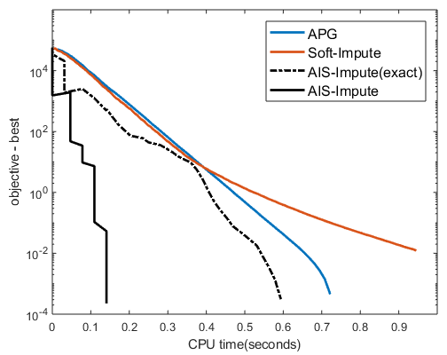
(a) $m=250$.

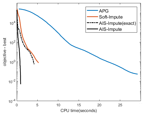
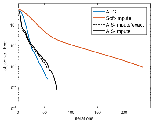
(b) $m=1000$.

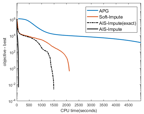
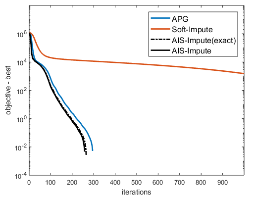
(c) $m=4000$.

Figure 1: Convergence of objective value on the synthetic data. Left: vs CPU time (in seconds); Right: vs number of iterations (note that AIS-Impute(exact) and AIS-Impute overlap with each other).

Table III also shows the NMSE results with post-processing (Section 3.6). Compared to the time used by the main algorithm (Figure 1), the post-processing time is small and can be ignored. Thus, post-processing is always performed in the sequel.

5.2 Recommender System

In this section, experiments are performed on two well-known benchmark data sets, MovieLens and Netflix.

MovieLens. The MovieLens data set (Table IV) contains ratings ($\{1,2,3,4,5\}$) of different users on movies. It has been commonly used in matrix completion experiments [13, 28]. We randomly use $50\%$ of the observed ratings for training, $25\%$ for validation and the rest for testing.

TABLE IV: MovieLens data sets used in the experiments.

	#users	#movies	# observed ratings
100K	943	1,682	100,000
1M	6,040	3,449	999,714
10M	69,878	10,677	10,000,054

TABLE V: Results on the MovieLens data sets. Note that TR and APG cannot converge in $10^{4}$ seconds on the 10M data set.

		100K		1M		10M
		RMSE	rank	RMSE	rank	RMSE	rank
factorization	LMaFit	0.896$\pm$0.011	3	0.827$\pm$0.002	6	0.819$\pm$0.001	12
	ASD	0.905$\pm$0.055	3	0.826$\pm$0.004	6	0.816$\pm$0.002	12
	R1MP	0.938$\pm$0.016	10	0.857$\pm$0.001	19	0.853$\pm$0.002	27
nuclear norm	active	0.880$\pm$0.003	8	0.821$\pm$0.001	16	0.803$\pm$0.001	72
minimization	boost	0.881$\pm$0.003	8	0.821$\pm$0.001	16	0.814$\pm$0.001	15
	Sketchy	0.889$\pm$0.003	8	0.821$\pm$0.001	48	0.826$\pm$0.001	60
	TR	0.884$\pm$0.002	8	0.820$\pm$0.001	20	—	—
	SSGD	0.886$\pm$0.011	8	0.849$\pm$0.006	16	0.858$\pm$0.014	45
	APG	0.880$\pm$0.003	8	0.820$\pm$0.001	16	—	—
	Soft-Impute	0.881$\pm$0.003	8	0.821$\pm$0.001	16	0.803$\pm$0.001	72
	ALT-Impute	0.882$\pm$0.003	8	0.823$\pm$0.001	16	0.805$\pm$0.001	45
	AIS-Impute	0.880$\pm$0.003	8	0.820$\pm$0.001	16	0.802$\pm$0.001	72

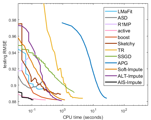
(a) 100K.

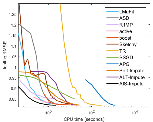
(b) 1M.

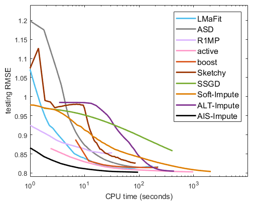
(c) 10M.

Figure 2: Testing RMSE vs CPU time (in seconds) on MovieLens data sets.

We compare AIS-Impute with the two most popular low-rank matrix learning approaches [1, 9], namely, factorization-based and nuclear-norm minimization methods. The factorization-based methods include (i) large scale matrix fit (“LMaFit”) [32], which uses alternative minimization with over-relaxation; (ii) alternative steepest descent (“ASD”) [33], which uses alternating steepest descent; (iii) rank-one matrix pursuit (“R1MP”) [34], which greedily pursues a rank-one basis in each iteration. The nuclear-norm minimization methods include (i) active subspace selection (“active”) [28], which uses the power method in each iteration to identify the active row and column subspaces; (ii) a boosting approach (“boost”) [31], which uses a variant of the Frank-Wolfe (FW) algorithm [45], with local optimization in each iteration using L-BFGS; (iii) sketchy decisions (“Sketchy”) [35], which is also a FW variant, and uses random matrix projection [17] to reduce the space and per-iteration time complexities; (iv) second-order trust-region algorithm (“TR”) [30], which alternates fixed-rank optimization and rank-one updates; (vi) stochastic gradient descent (“SSGD”) [37], which is a stochastic gradient descent algorithm; and (v) matrix completion based on fast alternating least squares (“ALT-Impute”) [36], which is a fast variant of Soft-Impute [13] that avoids SVD by alternating least squares. For all algorithms, parameters are tuned using the validation set. The algorithm is stopped when the relative change in objectives between consecutive iterations is smaller than ${10}^{-4}$.

For performance evaluation, as in [28, 13], we use (i) the root mean squared error on the test set: $\text{RMSE}=\|P_{\hat{\Omega}}(X-\hat{O})\|_{F}/(\|\hat{\Omega}\|_{1})^{\frac{1}{2}}$, where $X$ is the recovered matrix, and the testing ratings $\{\hat{O}_{ij}\}$ is indexed by the set $\hat{\Omega}$; and (ii) rank of $X$. The experiment is repeated 5 times and the average performance is reported.

Results are shown in Table V. As can be seen, AIS-Impute is consistently the fastest and has the lowest RMSE. On MovieLens-10M, TR and APG are not run as they are too slow. Figure 2 shows the testing RMSE with CPU time. As can be seen, Boost, TR, SSGD and APG are all very slow. Boost and TR need to solve an expensive subproblem in each iteration; SSGD has slow convergence; while APG requires SVD and does not utilize the “sparse plus low-rank” structure for fast matrix multiplication. ALT-Impute and LMaFit do not need SVT, and are faster than Soft-Impute. However, their nonconvex formulations have slow convergence, and are thus slower than AIS-Impute. Overall, AIS-Impute is the fastest, as it combines inexpensive iteration with fast convergence.

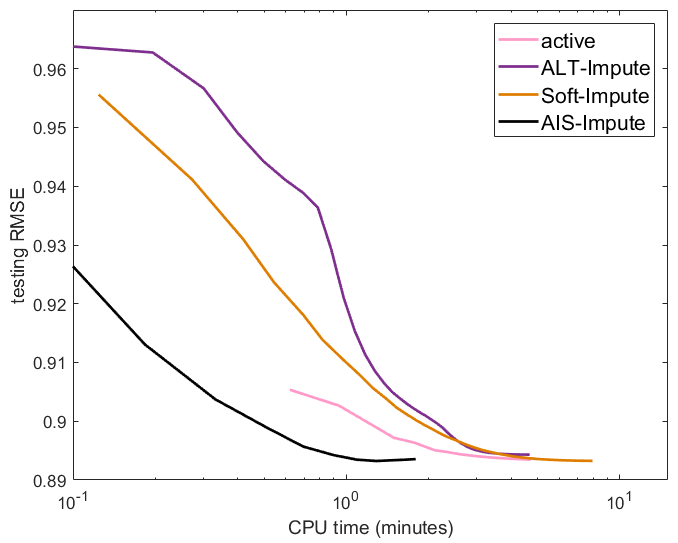
(a) $\lambda=\lambda_{0}/10$.

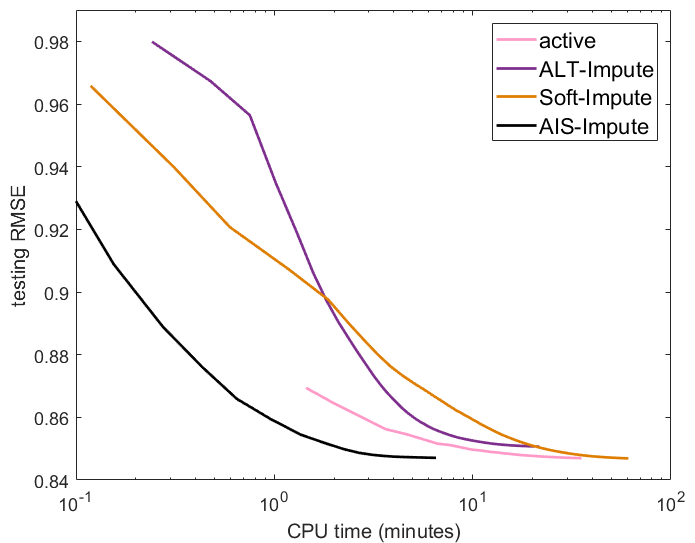
(b) $\lambda=\lambda_{0}/20$.

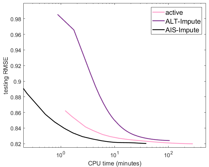
(c) $\lambda=\lambda_{0}/30$.

Figure 3: Testing RMSE vs CPU time (in minutes) on the Netflix data set, with various values for the regularization parameter $\lambda$.

Netflix. The Netflix data set contains ratings of 480,189 users on 17,770 movies. $1\%$ of the ratings matrix are observed. We randomly sample $50\%$ of the observed ratings for training, and the rest for testing.

We only compare with active subspace selection, ALT-Impute and Soft-Impute; while methods including boost, TR, SSGD, APG are slow and not compared. LMaFit solves a different optimization problem based on matrix factorization, and has worse recovery performance than AIS-Impute. Thus, it is also not compared. As in [13], several choices of the regularization parameter $\lambda$ are experimented.

Results are shown in Table VI. As in previous experiments, the RMSEs and ranks obtained by the various algorithms are similar. Figure 3 shows the plot of testing RMSE versus CPU time. As can be seen, AIS-Impute is again much faster.

TABLE VI: Results on the Netflix data set. The regularization parameter $\lambda$ in (1) is set as $\lambda_{0}/c$, where $\lambda_{0}=\|P_{\Omega}(O)\|_{F}$. Soft-Impute with $c=30$ is not run as it is very slow.

		RMSE	rank
$c=10$	active	0.894$\pm$0.001	3
	ALT-Impute	0.900$\pm$0.006	3
	Soft-Impute	0.893$\pm$0.001	3
	AIS-Impute	0.893$\pm$0.001	3
$c=20$	active	0.847$\pm$0.001	14
	ALT-Impute	0.850$\pm$0.001	14
	Soft-Impute	0.847$\pm$0.001	14
	AIS-Impute	0.847$\pm$0.001	14
$c=30$	active	0.820$\pm$0.001	116
	ALT-Impute	0.825$\pm$0.001	116
	AIS-Impute	0.820$\pm$0.001	116

5.3 Grayscale Images

In this section, we perform experiments on images from [18] (Figures 4(a)-4(c)). The pixels are normalized to zero mean and unit variance. Gaussian noise from $\mathcal{N}(0,0.05)$ is then added. In each image, 50% of the pixels are randomly sampled as observations (half for training and another half for validation). The task is to fill in the remaining 80% of the pixels. The experiment is repeated five times.

(a) rice (854 $\times$ 960).

(b) tree (800 $\times$ 800).

(c) wall (841 $\times$ 850).

Figure 4: Grayscale images used for matrix completion. Their sizes are shown in the bracket.

Table VII shows the testing RMSE and recovered rank. As can be seen, nuclear norm minimization is better in terms of RMSE (in particular, AIS-Impute, ALT-Impute, APG and boost are the best), though they require the use of higher ranks. Figure 5 shows the running time. As can be seen, AIS-Impute is consistently the fastest.

Figure 6 compares the difference between recovered images from all algorithms and the clean one on image tree. As can be seen, the difference on SSGD is the largest. Besides, LMaFit, ASD, and R1MP and SSGD also have larger errors than the rest. The observations on rice and wall are similar, however, due to space limitation, we do not show them here.

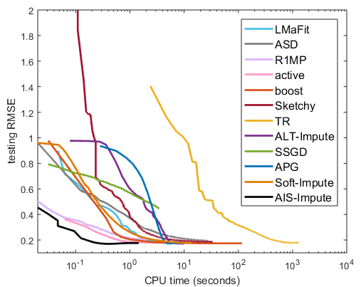
(a) rice.

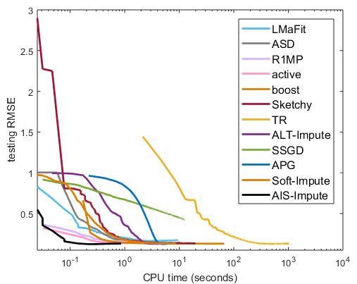
(b) tree.

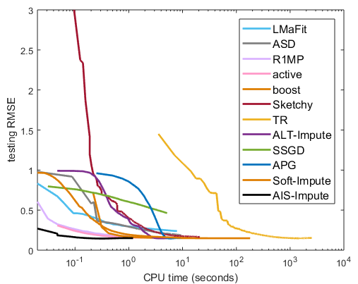
(c) wall.

Figure 5: Testing RMSE vs CPU time (in seconds) on grayscale images.

TABLE VII: Matrix completion results on grayscale images. CPU time is in seconds.

		rice		tree		wall
		RMSE	rank	RMSE	rank	RMSE	rank
factorization	LMaFit	0.189$\pm$0.002	45	0.174$\pm$0.013	25	0.238$\pm$0.004	50
	ASD	0.194$\pm$0.020	45	0.142$\pm$0.004	25	0.189$\pm$0.012	50
	R1MP	0.207$\pm$0.001	54	0.159$\pm$0.002	53	0.175$\pm$0.001	58
nuclear norm	active	0.176$\pm$0.002	100	0.130$\pm$0.002	71	0.150$\pm$0.002	101
minimization	boost	0.176$\pm$0.004	94	0.130$\pm$0.002	60	0.149$\pm$0.002	93
	Sketchy	0.186$\pm$0.007	89	0.134$\pm$0.002	41	0.157$\pm$0.008	88
	TR	0.179$\pm$0.001	150	0.131$\pm$0.002	103	0.151$\pm$0.001	149
	SSGD	0.447$\pm$0.058	96	0.424$\pm$0.037	60	0.463$\pm$0.023	96
	APG	0.176$\pm$0.001	96	0.130$\pm$0.002	60	0.151$\pm$0.001	96
	Soft-Impute	0.176$\pm$0.001	113	0.131$\pm$0.004	71	0.151$\pm$0.002	112
	ALT-Impue	0.176$\pm$0.004	96	0.130$\pm$0.004	71	0.150$\pm$0.001	95
	AIS-Impute	0.176$\pm$0.001	96	0.219$\pm$0.002	70	0.150$\pm$0.001	95

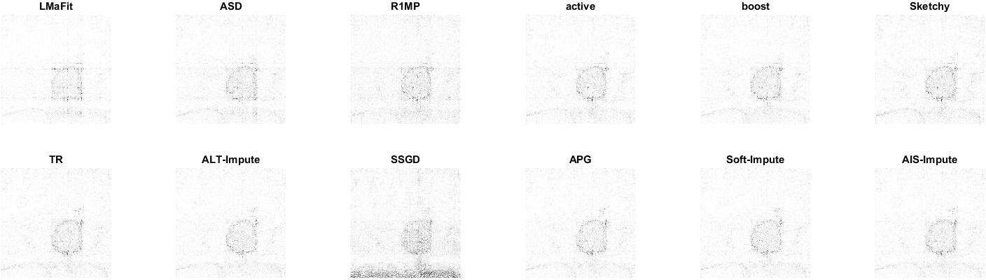
Figure 6: Comparison on the difference between reconstructed images and the clean one on image tree.

5.4 Nonconvex Regularization

In the following, we first perform experiments on (i) synthetic data, using the setup in Section 5.1 (with $m=250$ and $1000$); and (ii) the recommender data set MovieLens-100K, using the setup in Section 5.2. Three nonconvex low-rank regularizers are considered, namely, truncated nuclear norm (TNN) [18], capped-$\ell_{1}$ norm [42] and log-sum-penalty (LSP) [40].

For TNN, we compare three solvers: (i) TNNR(APG): the solver used in [18]; (ii) IRNN [6], which is a more recent proximal algorithm for optimization with nonconvex low-rank matrix regularizers (including the TNN); and (iii) the proposed AIS-Impute extension (denoted DC(AIS-Impute)), which replaces the original APG solver in [18] for the subproblem in TNNR with AIS-Impute. For capped-$\ell_{1}$ and LSP, two solvers are considered: (i) IRNN and (ii) the proposed AIS-Impute extension. As a further baseline, we also compare with (convex) nuclear norm regularization with the AIS-Impute solver. Experiments are repeated five times.

Results are shown in Table VIII. As can be seen, the errors obtained by nonconvex regularization (i.e., TNN, capped-$\ell_{1}$ and LSP) are much lower than those from convex nuclear norm regularization, illustrating the advantage of using nonconvex regularization. The performance obtained by the different nonconvex regularizers are comparable.

TABLE VIII: Comparison of nuclear norm regularization with various nonconvex regularizations.

		NMSE		RMSE
		synthetic ($m=250$)	synthetic ($m=1000$)	MovieLens-100K
nuclear norm	AIS-Impute	0.0098$\pm$0.0004	0.0092$\pm$0.0002	0.883$\pm$0.005
TNN	TNNR(APG)	0.0081$\pm$0.0004	0.0073$\pm$0.0001	0.851$\pm$0.002
	IRNN	0.0081$\pm$0.0004	0.0073$\pm$0.0001	0.853$\pm$0.004
	DC(AIS-Impute)	0.0081$\pm$0.0004	0.0073$\pm$0.0002	0.851$\pm$0.002
capped-$\ell_{1}$	IRNN	0.0089$\pm$0.0005	0.0074$\pm$0.0001	0.853$\pm$0.002
	DC(AIS-Impute)	0.0081$\pm$0.0004	0.0073$\pm$0.0002	0.852$\pm$0.005
LSP	IRNN	0.0083$\pm$0.0004	0.0076$\pm$0.0001	0.852$\pm$0.006
	DC(AIS-Impute)	0.0081$\pm$0.0004	0.0073$\pm$0.0002	0.850$\pm$0.002

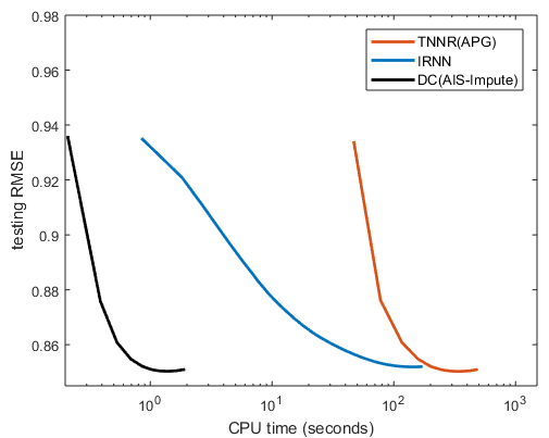
(a) TNN.

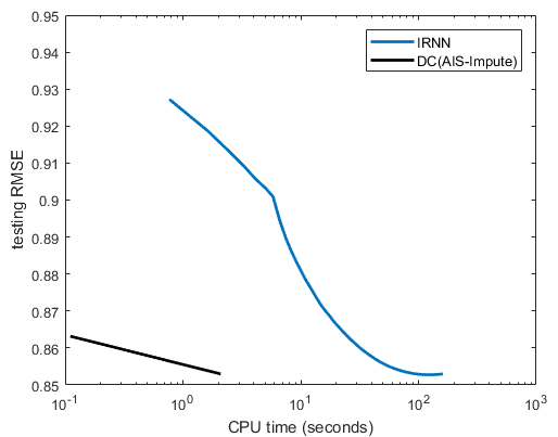
(b) capped-$\ell_{1}$.

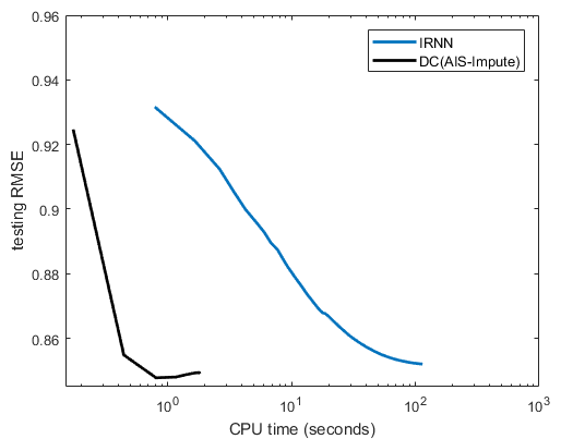
(c) LSP.

Figure 7: Convergence of testing RMSE vs CPU time (in seconds) on the MovieLens-100K data set.

5.5 Link Prediction

Given a graph with $m$ nodes and an incomplete adjacency matrix $O\in\{\pm 1\}^{m\times m}$, link prediction aims to recover a low-rank matrix $X\in\mathbb{R}^{m\times m}$ such that the signs of $X_{ij}$’s and $O_{ij}$’s agree on most of the observed entries. This is a binary matrix completion problem [3], and we use the logistic loss $\ell(X_{ij},O_{ij})\equiv\log\left(1+\exp(-X_{ij}O_{ij})\right)$ in (19).

Experiments are performed on the Epinions and Slashdot data sets [3] (Table IX). Each row/column of the matrix $O$ corresponds to a user (users with fewer than two observations are removed). For Epinions, $O_{ij}=1$ if user $i$ trusts user $j$, and $-1$ otherwise. Similarly for Slashdot, $O_{ij}=1$ if user $i$ tags user $j$ as friend, and $-1$ otherwise. As can be seen from previous sections, Boost, TR, SSGD, APG and Soft-Impute are all slow, and thus they are not considered here. Besides, LMaFit and ALT-Impute are designed for the square loss. Thus, comparison is performed with (i) active subspace selection; (ii) AIS-Impute; and (iii) AltMin: the alternative minimization approach used in [3]. We use 80% of the ratings for training, 10% for validation and the rest for testing. Let $X$ be the recovered matrix, and the test set $\{\hat{O}_{ij}\}$ be indexed by the set $\hat{\Omega}$. For performance evaluation, we use the (i) testing accuracy $\frac{1}{\|\hat{\Omega}\|_{1}}\sum_{(i,j)\in\hat{\Omega}}I(\text{sign}(X_{ij})=\hat{O}_{ij})$, where $I(\cdot)$ is the indicator function; and (ii) the rank of $X$. To reduce statistical variability, experimental results are averaged over 5 repetitions.

TABLE IX: Data sets for link prediction.

	#rows	#columns	#signs
Epinions	84,601	48,091	505,074
Slashdot	70,284	32,188	324,745

Results are shown in Table X and Figure 8 shows the testing accuracy with CPU time. As can be seen, active and AIS-Impute have slightly better accuracies than AltMin, and AIS-Impute is the fastest.

TABLE X: Performance on link prediction.

		accuracy	rank
Epinions	active	0.939$\pm$0.002	12
	AltMin	0.936$\pm$0.002	41
	AIS-Impute	0.940$\pm$0.001	12
Slashdot	active	0.844$\pm$0.001	16
	AltMin	0.839$\pm$0.002	39
	AIS-Impute	0.843$\pm$0.001	16

TABLE XI: Tensor completion results on the synthetic data. Here, sparsity is the proportion of observed entries, and post-processing time is in seconds.

		NMSE
		no post-processing	with post-processing	rank	post-processing time
$m=125$	APG	0.0162$\pm$0.0015	0.0100$\pm$0.0006	3,3,0	0.1
(sparsity: 62.4%)	Soft-Impute	0.0162$\pm$0.0014	0.0100$\pm$0.0005	3,3,0	0.1
	AIS-Impute(exact)	0.0161$\pm$0.0015	0.0100$\pm$0.0005	3,3,0	0.1
	AIS-Impute	0.0159$\pm$0.0011	0.0099$\pm$0.0004	3,3,0	0.1
$m=500$	APG	0.0166$\pm$0.0007	0.0105$\pm$0.0004	3,3,0	0.1
(sparsity: 16.0%)	Soft-Impute	0.0168$\pm$0.0007	0.0106$\pm$0.0004	3,3,0	0.1
	AIS-Impute(exact)	0.0167$\pm$0.0006	0.0104$\pm$0.0003	3,3,0	0.1
	AIS-Impute	0.0167$\pm$0.0007	0.0105$\pm$0.0003	3,3,0	0.1
$m=2000$	APG	0.0162$\pm$0.0013	0.0105$\pm$0.0006	3,3,0	0.5
(sparsity: 3.9%)	Soft-Impute	0.0168$\pm$0.0016	0.0109$\pm$0.0011	3,3,0	0.4
	AIS-Impute(exact)	0.0161$\pm$0.0012	0.0104$\pm$0.0007	3,3,0	0.4
	AIS-Impute	0.0161$\pm$0.0012	0.0104$\pm$0.0007	3,3,0	0.1

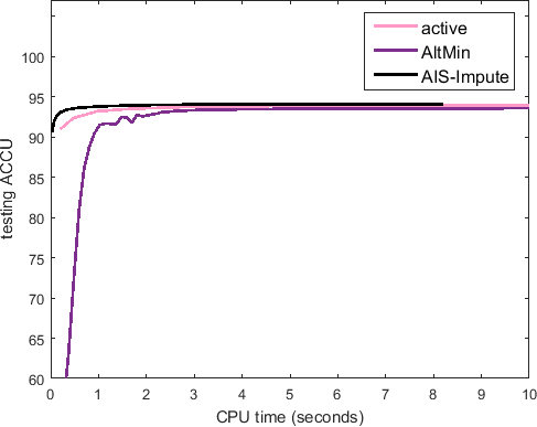
(a) Epinions.

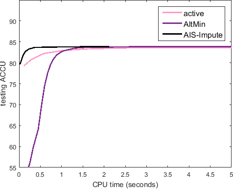
(b) Slashdot.

Figure 8: Testing accuracy vs CPU time (in seconds) on the Epinions and Slashdot data sets.

5.6 Tensor Completion: Synthetic Data

In this section, we perform tensor completion experiments with synthetic data. The ground-truth data tensor (of size $m\times m\times 3$) is generated as ${{\boldsymbol{\mathbf{\mathscr{{O}}}}}}={{\boldsymbol{\mathbf{\mathscr{{C}}}}}}\times_{1}A_{1}\times_{2}A_{2}\times_{3}A_{3}$, where the elements of $A_{1}\in\mathbb{R}^{m\times 3}$, $A_{2}\in\mathbb{R}^{m\times 3}$, $A_{3}\in\mathbb{R}^{3\times 3}$ and the core tensor ${{\boldsymbol{\mathbf{\mathscr{{C}}}}}}\in\mathbb{R}^{3\times 3}$ are all sampled i.i.d. from the standard normal distribution $\mathcal{N}(0,1)$, and $\times_{k}$ is the $k$-mode product. Thus, ${{\boldsymbol{\mathbf{\mathscr{{O}}}}}}$ is low-rank for the first two mode but not for the third. Noise ${{\boldsymbol{\mathbf{\mathscr{{G}}}}}}$, with elements sampled i.i.d. from the normal distribution $\mathcal{N}(0,0.05)$, is then added. A total number of $\Omega=45m\log(m)$ random elements in ${{\boldsymbol{\mathbf{\mathscr{{O}}}}}}$ are observed. Half of them are used for training, and the other half for validation. On testing, we perform evaluation on the unobserved entries and use the same criteria as in Section 5.1, i.e., NMSE and recovered rank in each mode.

Similar to Section 5.1, we compare the following algorithms: (i) APG; (ii) extension of Soft-Impute to tensor completion, which is based on Section 4.2; (iii) the proposed algorithm with exact SVD (AIS-Impute(exact)); and (iv) the proposed algorithm which uses power method to approximate SVT (AIS-Impute).

As suggested in [22], we set $(\lambda_{1},\lambda_{2},\lambda_{3})$ in the scaled latent nuclear norm to $(1,1,\frac{\sqrt{m}}{\sqrt{3}})\lambda$. Thus, the only tunable parameter is $\lambda$, which is obtained by grid search using the validation set. We also vary $m$ in $\{125,500,2000\}$. Experimental results are averaged over 5 repetitions.

Results on NMSE and rank are shown in Table XI. As can be seen, APG, Soft-Impute, AIS-Impute(exact) and AIS-Impute have comparable performance. The plots of objective value vs time and iterations are shown in Figure 9. In terms of iterations, APG, AIS-Impute(exact) and AIS-Impute have similar behavior as they all have $O(1/T^{2})$ convergence rate. These also agree with the matrix case in Section 5.1. In terms of time, as APG does not utilize the “sparse plus low-rank” structure, it is slower than AIS-Impute(exact) and AIS-Impute. AIS-Impute is the fastest, as it has both fast $O(1/T^{2})$ convergence rate and low per-iteration complexity.

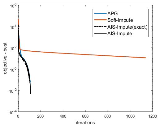
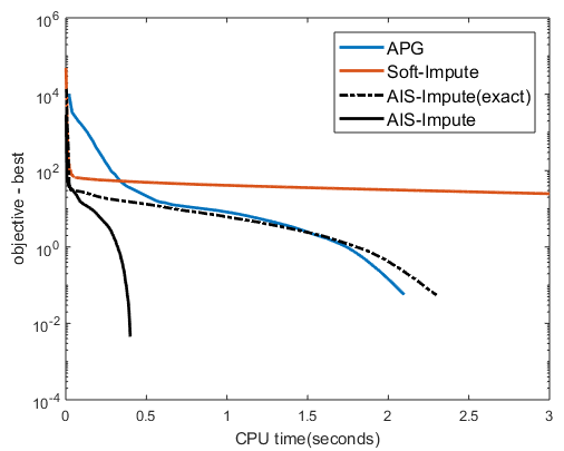
(a) $m=125$.

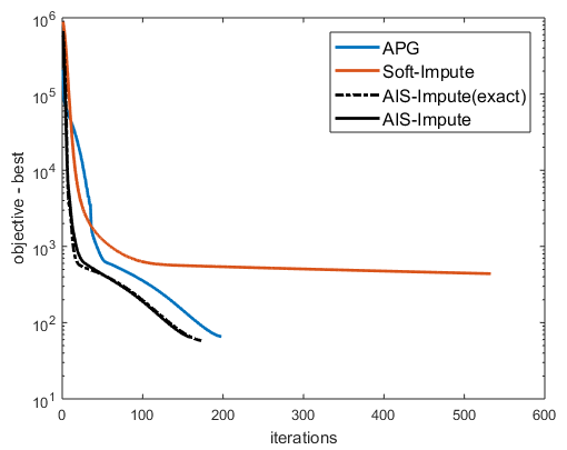
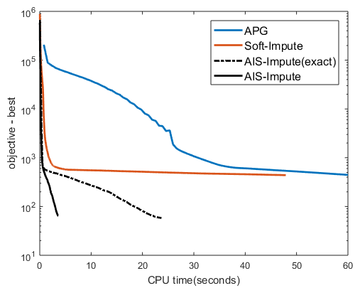
(b) $m=500$.

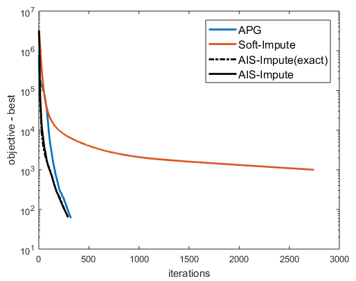
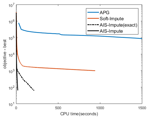
(c) $m=2000$.

Figure 9: Convergence of objective value on the synthetic tensor data. Left: vs number of iterations; Right: vs CPU time (in seconds).

Performance with post-processing in Section 4.5 is shown in Table XI. As can be seen, it is very efficient and improves NMSE. Thus, we always perform post-processing in the sequel.

5.7 Multi-Relational Link Prediction

In this section, we perform experiments on the YouTube data set [46]. It contains 15,088 users, and describes five types of user interactions: contact, number of shared friends, number of shared subscriptions, number of shared subscribers, and the number of shared favorite videos. Thus, it forms a $15088\times 15088\times 5$ tensor, with a total of $27,257,790$ nonzero elements. Following [3], we formulate multi-relational link prediction as a tensor completion problem. As the observations are real-valued, we use the square loss in (30). Besides AIS-Impute (Algorithm 4), we also compare with the following state-of-the-art non-proximal-based tensor completion algorithms: (i) geometric nonlinear CG for tensor completion (denoted “GeomCG”) [47]: a gradient descent approach with gradients restricted on the Riemannian manifold; (ii) An alternating direction method of multipliers approach (denoted “ADMM(overlap)”) [20], which solves the overlapping nuclear norm regularized tensor completion problem; (iii) fast low rank tensor completion (denoted “FaLRTC”) [4]: It smooths the overlapping nuclear norm and then solves the relaxed problem with accelerated gradient descent; and (iv) tensor completion by parallel matrix factorization (denoted “TMac”) [48]: An extension of LMaFit [32] to tensor completion, which performs simultaneous low-rank matrix factorizations to all mode matricizations.

YouTube Subset. First, we perform experiments on a small YouTube subset, obtained by random selecting 1000 users (leading to $12,101$ observations). We use $50\%$ of the observations for training, another $25\%$ for validation and the remaining for testing. Let ${{\boldsymbol{\mathbf{\mathscr{{X}}}}}}$ be the recovered tensor, and the testing ratings $\hat{O}_{ij}$ be indexed by the set $\hat{\Omega}$. For performance evaluation, we use (i) the testing root mean squared error $\text{RMSE}=\sqrt{\|P_{\hat{\Omega}}({{\boldsymbol{\mathbf{\mathscr{{X}}}}}}-\hat{{{\boldsymbol{\mathbf{\mathscr{{O}}}}}}})\|_{F}^{2}/\|\hat{\Omega}\|_{1}}$; and (ii) rank of the unfolded matrix in each mode. The experiments are repeated five times.

Performance is shown in Table XII and Figure 10(a) shows the time comparison. ADMM(overlap) and FaLRTC have similar recovery performance, but are all very slow due to usage of the SVD. As the overlapping nuclear norm is smoothed in FaLRTC, its cannot exactly recover a low-rank tensor. TMac is fast, but has the worst recovery performance. AIS-Impute enjoys fast speed and good recovery performance.

TABLE XII: Results on the YouTube subset. The rank is for each mode.

	RMSE	rank
GeomCG	0.672$\pm$0.050	7, 7, 5
ADMM(overlap)	0.690$\pm$0.030	142, 142, 5
FaLRTC	0.672$\pm$0.032	1000, 1000, 5
TMac	0.786$\pm$0.027	4, 4, 0
AIS-Impute	0.616$\pm$0.029	33, 33, 0

Full YouTube Data. Next, we perform experiments on the full YouTube data set with the same setup. As ADMM(overlap) and FaLRTC are too slow, we only compare with GeomCG, TMac and AIS-Impute. Experiments are repeated five times.

Results are shown in Table XIII, and Figure 10(b) shows the time. TMac has much worse performance than GeomCG and AIS-Impute. GeomCG is based on the (nonconvex) Turker decomposition, and its convergence rate is unknown. Moreover, its iteration time complexity has a worse dependency on the tensor rank than AIS-Impute ($\prod_{i=1}^{D}r_{t}^{d}$ vs $\sum_{i=1}^{D}r_{t}^{d}$), and thus GeomCG becomes very slow when the tensor rank is large. Overall, AIS-Impute has fast speed and good recovery performance.

TABLE XIII: Results on the full YouTube dataset. The rank is for each mode.

	RMSE	rank
GeomCG	0.388$\pm$0.001	51, 51, 5
TMac	0.611$\pm$0.007	10, 10, 0
AIS-Impute	0.369$\pm$0.006	70, 70, 0

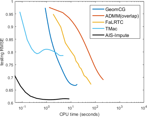
(a) data subset.

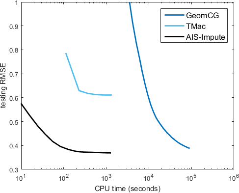
(b) full data set.

Figure 10: Testing RMSE vs CPU time on the Youtube data set.

6 Conclusion

In this paper, we show that Soft-Impute, as a proximal algorithm, can be accelerated without losing the “sparse plus low-rank” structure crucial to its efficiency. To further reduce the per-iteration time complexity, we proposed an approximate-SVT scheme based on the power method. Theoretical analysis shows that the proposed algorithm still enjoys the fast $O(1/T^{2})$ convergence rate. We also extend the proposed algorithm for low-rank tensor completion with the scaled latent nuclear norm regularizer. Again, the “sparse plus low-rank” structure can be preserved and a convergence rate of $O(1/T^{2})$ can be obtained. The proposed algorithm can be further extended to nonconvex low-rank regularizers, which have better empirical performance than the convex nuclear norm regularizer. Extensive experiments on both synthetic and real-world data sets show that the proposed algorithm is much faster than the state-of-the-art.

Quanming Yao obtained his Ph.D from Computer Science and Engineer Department of Hong Kong University of Science and Technology (HKUST) in 2018, and bachelor degree in Electronic and Information Engineering from the Huazhong University of Science and Technology (HUST) in 2013. His research interests focus on machine learning. Currently, he is a research scientist in 4Paradigm Inc. (Beijing, China). He was awarded as Qiming star of HUST in 2012, Tse Cheuk Ng Tai research excellence prize from HKUST in 2015 and Google PhD fellowship (machine learning) in 2016.

James T. Kwok received the PhD degree in computer science from the Hong Kong University of Science and Technology in 1996. He was with the Department of Computer Science, Hong Kong Baptist University, Hong Kong, as an assistant professor. He is currently a professor in the Department of Computer Science and Engineering, Hong Kong University of Science and Technology. His research interests include kernel methods, machine learning, example recognition, and artificial neural networks. He received the IEEE Outstanding 2004 Paper Award, and the Second Class Award in Natural Sciences by the Ministry of Education, People’s Republic of China, in 2008. He has been a program cochair for a number of international conferences, and served as an associate editor for the IEEE Transactions on Neural Networks and Learning Systems and Neurocomputing journal.

Appendix A Proofs

A.1 Proposition 3.1

Proof.

For any $X,Y\in\mathbb{R}^{m\times n}$,

$$\|\nabla f(X)-\nabla f(Y)\|_{F}^{2}$$

$$=\sum_{(i,j)\in\Omega}\left[\frac{d\ell(X_{ij},O_{ij})}{dX_{ij}}-\frac{d\ell(Y_{ij},O_{ij})}{dY_{ij}}\right]^{2}$$

$$\leq\sum_{(i,j)\in\Omega}\rho^{2}(X_{ij}-Y_{ij})^{2}$$ (37)

$$\leq\rho^{2}\|X-Y\|_{F}^{2},$$

where (37) follows from the fact that $\ell$ is $\rho$-Lipschitz smooth. Thus, $f(X)$ is $\rho$-Lipschitz smooth. ∎

A.2 Proposition 3.3

Proof.

First, we introduce the following theorem.

Theorem A.1 (Separation theorem [49]).

Let $A\in\mathbb{R}^{m\times n}$ and $B\in\mathbb{R}^{m\times r}$ with $B^{\top}B=I$. Then

$$\sigma_{i}\left(B^{\top}A\right)\leq\sigma_{i}(A),\;\text{for}\;i=1,\dots,\min(r,n).$$

Let the SVD of $Z$ be $U\Sigma V^{\top}$. $Z$ can then be rewritten as

$$Z=\left[U_{\breve{k}_{t}};U_{\bot}\right]\begin{bmatrix}\Sigma_{\breve{k}_{t}}&\\ &\Sigma_{\bot}\end{bmatrix}\left[V_{\breve{k}_{t}};V_{\bot}\right]^{\top},$$ (38)

where $U_{\breve{k}_{t}}$ contains the $\breve{k}_{t}$ leading columns of $U$, and $U_{\bot}$ the remaining columns. Similarly, $\Sigma_{\breve{k}_{t}}$ (resp. $V_{\breve{k}_{t}}$) contains the $\breve{k}_{t}$ leading eigenvalues (resp. columns) of $\Sigma$ (resp. $V$). Then, let

$$\tilde{u}_{i}=Q^{\top}u_{i}\text{\quad and \quad}\tilde{v}_{i}=v_{i},$$ (39)

where $u_{i}$ (resp. $v_{i}$) is the $i$th column of $U$ (resp. $V$). For $i=1,\cdots,\breve{k}_{t}$, we have

$$\tilde{u}_{i}^{\top}\left(Q^{\top}Z\right)\tilde{v}_{i} = U_{i}^{\top}\left(QQ^{\top}\right)ZV_{i}$$ (40)

$$= U_{i}^{\top}ZV_{i}$$

$$= \sigma_{i}(Z),$$ (41)

where (40) is due to $\text{span}(U_{\breve{k}_{t}})\subseteq\text{span}(Q)$. Hence,

$$\sigma_{i}\left(Q^{\top}Z\right) = \sigma_{i}(Z),\text{\;for\;}i=1,\cdots,\breve{k}_{t}$$ (42)

From Theorem A.1, by substituting $Q=B$ and $A=Z$, we have $\sigma_{i}(Q^{\top}Z)\leq\sigma_{i}(Z)$. Combining with (42), we obtain that the rank-$\breve{k}_{t}$ SVD of $Q^{\top}Z$ is $(Q^{\top}U_{\breve{k}_{t}})\Sigma_{\breve{k}_{t}}V_{\breve{k}_{t}}^{\top}$, with the corresponding left and right singular vectors contained in $Q^{\top}U_{\breve{k}_{t}}$ and $V_{\breve{k}_{t}}$, respectively.

Again, by Theorem A.1, we have

$$\sigma_{\breve{k}_{t}+1}\left(Q^{\top}Z\right)\leq\sigma_{\breve{k}_{t}+1}(Z)\leq\mu.$$

Besides, using (38),

$$\sigma_{i}\left(Q^{\top}Z\right)=\max_{u,v}u\left(Q^{\top}U_{\breve{k}_{t}}\Sigma_{\breve{k}_{t}}V_{\breve{k}_{t}}^{\top}+Q^{\top}U_{\bot}\Sigma_{\bot}V_{\bot}^{\top}\right)v.$$

Since the first $\breve{k}_{t}$ singular values are from the term $Q^{\top}U_{\breve{k}_{t}}\Sigma_{\breve{k}_{t}}V_{\breve{k}_{t}}$, then

$$\sigma_{\breve{k}_{t}+1}\left(Q^{\top}Z\right)=\max_{u,v}u^{\top}\left(Q^{\top}U_{\bot}\Sigma_{\bot}V_{\bot}^{\top}\right)v\leq\mu.$$ (43)

Then,

$$\text{SVT}_{\mu r}(Q^{\top}Z)$$

$$=\text{SVT}_{\mu r}\left(Q^{\top}U_{\breve{k}_{t}}\Sigma_{\breve{k}_{t}}V_{\breve{k}_{t}}^{\top}+Q^{\top}U_{\bot}\Sigma_{\bot}V_{\bot}^{\top}\right)$$

$$=\text{SVT}_{\mu r}\left(Q^{\top}U_{\breve{k}_{t}}\Sigma_{\breve{k}_{t}}V_{\breve{k}_{t}}^{\top}\right)+\text{SVT}_{\mu r}\left(Q^{\top}U_{\bot}\Sigma_{\bot}V_{\bot}^{\top}\right)$$ (44)

$$=\text{SVT}_{\mu r}\left(Q^{\top}U_{\breve{k}_{t}}\Sigma_{\breve{k}_{t}}V_{\breve{k}_{t}}^{\top}\right).$$ (45)

where (44) follows from that $Q^{\top}U_{\breve{k}_{t}}$ (resp. $V_{\breve{k}_{t}}$) is orthogonal to $QU_{\bot}$ (resp. $V_{\bot}$). (43) shows that there are only $\breve{k}_{t}$ singular values in $Q^{\top}Z$ larger than $\mu$. Thus, $\text{SVT}_{\mu r}{Q^{\top}U_{\bot}\Sigma_{\bot}V_{\bot}^{\top}}=0$ and we get (45). Finally,

$$Q\text{SVT}_{\mu r}\left(Q^{\top}Z\right) =Q\left(Q^{\top}U_{\breve{k}_{t}}\text{SVT}_{\mu r}{\Sigma_{\breve{k}_{t}}}V_{\breve{k}_{t}}^{\top}\right)$$

$$=U_{\breve{k}_{t}}\text{SVT}_{\mu r}\left(\Sigma_{\breve{k}_{t}}\right)V_{\breve{k}_{t}}^{\top}$$ (46)

$$=\text{SVT}_{\mu r}(Z),$$ (47)

where (46) comes from $\text{span}(U_{\breve{k}_{t}})\subseteq\text{span}(Q)$; (47) comes from that rank-$\breve{k}_{t}$ SVD of $Z$ is $U_{\breve{k}_{t}}\Sigma_{\breve{k}_{t}}V_{\breve{k}_{t}}^{\top}$ and $Z$ only has $\breve{k}_{t}$ singular values larger than $\mu$. ∎

A.3 Proposition 3.4

Before proof of Proposition 3.4, we first introduce some Lemmas (Lemma A.2, A.4, A.3 and A.7) and Propositions (Proposition A.5 and A.6).

Lemma A.2 ([10]).

For any matrices $A$ and $B$, $\left\|\text{SVT}_{\lambda}(A)-\text{SVT}_{\lambda}(B)\right\|_{F}\leq\left\|A-B\right\|_{F}$.

Let $Z_{t}^{*}\equiv\text{SVT}_{\mu\lambda}(\breve{Z}_{t})$, $\beta_{t}\equiv\|\breve{Z}_{t}\|_{F}$ and $\eta_{t}=\frac{\sigma_{k+1}(\breve{Z}_{t})}{\sigma_{k}(\breve{Z}_{t})}$.

Lemma A.3 ([17]).

Let the input to Algorithm 1 be $\breve{Z}_{t}$, and its top $k$ left singular vectors be contained in $U_{k}$. Then, for $j=0,1,2,\dots$,

$$\|Q_{j}{Q_{j}}^{\top}-U_{k}U_{k}^{\top}\|_{F}\leq\eta_{t}^{j}\alpha_{t},$$

where $\alpha_{t}=\|Q_{0}{Q_{0}}^{\top}-U_{k}U_{k}^{\top}\|_{F}$ and $Q_{0}$ is the span of $\breve{Z}_{t}R_{t}$.

Lemma A.4.

For output $\tilde{X}=(QU)\Sigma V^{\top}$ from Algorithm 2, we have $\|\tilde{X}-Z_{t}^{*}\|_{F}\leq\|U_{k}U_{k}^{\top}-QQ^{\top}\|_{F}\beta_{t}$.

Proof.

From Proposition 3.3,

$$Z_{t}^{*}-\tilde{X} = \text{SVT}_{\mu\lambda}(\breve{Z}_{t})-Q\text{SVT}_{\mu\lambda}(Q^{\top}\breve{Z}_{t})$$

$$= \text{SVT}_{\mu\lambda}(U_{k}U_{k}^{\top}\breve{Z}_{t})-\text{SVT}_{\mu\lambda}(QQ^{\top}\breve{Z}_{t}).$$

Using Lemma A.2 and the Cauchy’s inequality,

$$\|\tilde{X}-Z_{*}\|_{F} = \|\text{SVT}_{\mu\lambda}(U_{k}U_{k}^{\top}\breve{Z}_{t})-\text{SVT}_{\mu\lambda}(QQ^{\top}\breve{Z}_{t})\|_{F}$$

$$\leq \|(U_{k}U_{k}^{\top}-QQ^{\top})\breve{Z}_{t}\|_{F}$$

$$\leq \|U_{k}U_{k}^{\top}-QQ^{\top}\|_{F}\beta_{t},$$

and result follows. ∎

Proposition A.5.

Let $G_{t}\in\partial h_{\mu\lambda\|\cdot\|_{*}}(\tilde{X};\breve{Z}_{t})$, then $\|G_{t}\|_{F}$ is upper-bounded by a constant $\gamma_{t}$.

Proof.

Let the reduced SVD of $\tilde{X}$ be $U\Sigma V^{\top}$ (only positive singular values are contained). By the definition of subgradient of the nuclear norm [9],

$$\partial h_{\mu\lambda\|\cdot\|_{*}}(\tilde{X};\breve{Z}_{t})=\tilde{X}-\breve{Z}_{t}+\mu\lambda(UV^{\top}+W),$$

where

$$W^{\top}U=0,\;WV=0,\text{ and }\|W\|_{\infty}\leq 1.$$ (48)

Thus,

$$\|G_{t}\|_{F} =\|\tilde{X}-\breve{Z}_{t}+\mu\lambda(UV^{\top}+W)\|_{F}$$

$$\leq\|\tilde{X}-\breve{Z}_{t}\|_{F}+\mu\lambda\|UV^{\top}+W\|_{F}.$$ (49)

For the first term in (49),

$$\|\tilde{X}-\breve{Z}_{t}\|_{F}$$ (50)

$$= \|\tilde{X}-Z_{t}^{*}+Z_{t}^{*}-\breve{Z}_{t}\|_{F}$$

$$\leq \|\tilde{X}-Z_{t}^{*}\|_{F}+\|Z_{t}^{*}-\breve{Z}_{t}\|_{F}$$

$$= \|Z_{t}^{*}-\breve{Z}_{t}\|_{F}+\|Z_{t}^{*}-Q\text{SVT}_{\mu\lambda}(Q^{\top}\breve{Z}_{t})\|_{F}$$

$$= \|Z_{t}^{*}-\breve{Z}_{t}\|_{F}+\|Z_{t}^{*}-\tilde{X}\|_{F}$$

$$\leq \|Z_{t}^{*}-\breve{Z}_{t}\|_{F}+\|U_{k}U_{k}^{\top}-QQ^{\top}\|_{F}\beta_{t}$$

$$\leq \|Z_{t}^{*}-\breve{Z}_{t}\|_{F}+\alpha_{t}\beta_{t}.$$ (51)

Here, (50) follows from Lemma A.4, and (51) from Lemma A.3. As $\|W\|_{\infty}\leq 1$ from (48), thus

$$\|W\|_{F}=\sqrt{\sum_{i=1}^{m}\sigma_{i}^{2}(W)}\leq\sqrt{m}.$$

For the second term in (49), then

$$\|UV^{\top}+W\|_{F} \leq\sqrt{\,\text{tr}(U^{\top}UV^{\top}V)}+\|W\|_{F}$$

$$\leq\sqrt{k_{t}}+\sqrt{m}\leq 2\sqrt{m}.$$ (52)

Combining (51) and (52), by Lemma A.3:

$$\|G_{t}\|_{F}\leq 2\mu\lambda\sqrt{m}+\|Z_{t}^{*}-\breve{Z}_{t}\|_{F}+\alpha_{t}\beta_{t}.$$ (53)

Since $Z_{t}^{*}$ is independent of $\tilde{X}$, $\|Z_{t}^{*}-\breve{Z}_{t}\|_{F}$ is a constant. Hence, $\|G_{t}\|_{F}$ is upper bounded by

$$\gamma_{t}=2\mu\lambda\sqrt{m}+\|Z_{t}^{*}-\breve{Z}_{t}\|_{F}+\alpha_{t}\beta_{t},$$

which a constant. ∎

Proposition A.6.

Assume that $k_{t}\geq\breve{k}_{t}$. Let $h_{\mu\lambda\|\cdot\|_{*}}(\tilde{X};\breve{Z}_{t})$ be as defined in (8). Then, for Algorithm 2, we have

$$h_{\mu\lambda\|\cdot\|_{*}}(\tilde{X};\breve{Z}_{t})\leq h_{\mu\lambda\|\cdot\|_{*}}(Z_{t}^{*};\breve{Z}_{t})+\alpha_{t}\beta_{t}\gamma_{t}\eta_{t}^{J}.$$

Proof.

As $h$ is convex,

$$h_{\mu\lambda\|\cdot\|_{*}}(\tilde{X};\breve{Z}_{t})\leq h_{\mu\lambda\|\cdot\|_{*}}(Z_{t}^{*};\breve{Z}_{t})+\,\text{tr}((\tilde{X}-Z_{t}^{*})^{\top}G_{t})$$ (54)

where $G_{t}\in\partial h_{\mu\lambda\|\cdot\|_{*}}(\tilde{X};\breve{Z}_{t})$. Next, we bound the second term on the r.h.s. of (54).

$$\,\text{tr}((\tilde{X}-Z_{t}^{*})^{\top}G_{t}) \leq \|\tilde{X}-Z_{t}^{*}\|_{F}\|G_{t}\|_{F}$$ (55)

$$\leq \gamma_{t}\|\tilde{X}-Z_{t}^{*}\|_{F}$$

$$\leq \gamma_{t}\beta_{t}\|QQ^{\top}-U_{k}U_{k}^{\top}\|_{F}$$ (56)

$$\leq \eta_{t}^{J}(\alpha_{t}\beta_{t}\gamma_{t}).$$ (57)

Here, (55) follows from Proposition A.5; (56) from Lemma A.4; and (57) from Lemma A.3. Result follows on combining (54) and (57). ∎

Lemma A.7.

If $\{F(X_{t})\}$ is upper-bounded where $F$ is the objective at (19), then $\|X_{t}\|_{F}$ from Algorithm 3 is upper-bounded.

Proof.

As $\{F(X_{t})\}$ is upper bounded and note that

$$F(X)\rightarrow+\infty\Leftrightarrow\|X\|_{F}\rightarrow+\infty.$$

for (19), then $\{\|X_{t}\|_{F}\}$ is also upper bounded. ∎

Now, we are ready to prove Proposition 3.4. As $\alpha_{t}$, $\beta_{t}$ and $\gamma_{t}$ only depend on $X_{t}$, from Lemma A.7, they are all upper bounded. Let $q=\sup_{t}\alpha_{t}\beta_{t}\gamma_{t}$, and $q<\infty$ is a constant. Then by Proposition A.6, and note that Algorithm 2 is run for $t$ iterations at $t$th loop of Algorithm 3. Let $\eta=\max_{t}\eta_{t}\in(0,1)$, we have

$$h_{\mu\lambda\|\cdot\|_{*}}(X_{t+1};\breve{Z}_{t})\leq h_{\mu\lambda\|\cdot\|_{*}}(Z_{t}^{*};\breve{Z}_{t})+\varepsilon_{t}.$$

Hence, $\varepsilon_{t}=q\eta^{t}$ decays at a linear rate.

A.4 Theorem 3.5

Proof.

From Proposition 3.4, $\varepsilon_{t}$ decays at a linear rate. Moreover, there is no error on the computation of gradient. Thus, conditions in Proposition 2.1 are satisfied, and Algorithm 3 converges with a rate of $O(1/T^{2})$. ∎

A.5 Proposition 4.1

Proof.

Note that

$$\!\!\min_{{{\boldsymbol{\mathbf{\mathscr{{X}}}}}}^{1},\dots,{{\boldsymbol{\mathbf{\mathscr{{X}}}}}}^{D}}\!\frac{1}{2}\|[{{\boldsymbol{\mathbf{\mathscr{{X}}}}}}^{1},\dots,{{\boldsymbol{\mathbf{\mathscr{{X}}}}}}^{D}]-[\breve{{{\boldsymbol{\mathbf{\mathscr{{Z}}}}}}}_{t}^{1},\dots,\breve{{{\boldsymbol{\mathbf{\mathscr{{Z}}}}}}}_{t}^{D}]\|_{F}^{2}\!+\!\mu\sum_{d=1}^{D}\lambda_{d}\|{{\boldsymbol{\mathbf{\mathscr{{X}}}}}}^{d}_{{\left\langle d\right\rangle}}\|_{*}$$

$$=\sum_{d=1}^{D}\min_{{{\boldsymbol{\mathbf{\mathscr{{X}}}}}}^{d}}\frac{1}{2}\|{{\boldsymbol{\mathbf{\mathscr{{X}}}}}}^{d}-\breve{{{\boldsymbol{\mathbf{\mathscr{{Z}}}}}}}_{t}^{d}\|_{F}^{2}+\mu\lambda_{d}\|{{\boldsymbol{\mathbf{\mathscr{{X}}}}}}^{d}_{{\left\langle d\right\rangle}}\|_{*},$$

$$=\sum_{d=1}^{D}\min_{{{\boldsymbol{\mathbf{\mathscr{{X}}}}}}^{d}}\frac{1}{2}\|{{\boldsymbol{\mathbf{\mathscr{{X}}}}}}^{d}_{{\left\langle d\right\rangle}}-(\breve{{{\boldsymbol{\mathbf{\mathscr{{Z}}}}}}}_{t}^{d})_{{\left\langle d\right\rangle}}\|_{F}^{2}+\mu\lambda_{d}\|{{\boldsymbol{\mathbf{\mathscr{{X}}}}}}^{d}_{{\left\langle d\right\rangle}}\|_{*}.$$ (58)

The ${{\boldsymbol{\mathbf{\mathscr{{X}}}}}}^{d}$’s in (58) are independent of each other, and

$$(\text{SVT}_{\mu\lambda_{d}}(\breve{{{\boldsymbol{\mathbf{\mathscr{{Z}}}}}}}_{{\left\langle d\right\rangle}}^{d}))_{{\left\langle d\right\rangle}}\!=\!\arg\min_{{{\boldsymbol{\mathbf{\mathscr{{X}}}}}}^{d}}\frac{1}{2}\|{{\boldsymbol{\mathbf{\mathscr{{X}}}}}}^{d}_{{\left\langle d\right\rangle}}-\breve{{{\boldsymbol{\mathbf{\mathscr{{Z}}}}}}}^{d}_{{\left\langle d\right\rangle}}\|_{F}^{2}\!+\!\mu\lambda_{d}\|{{\boldsymbol{\mathbf{\mathscr{{X}}}}}}^{d}_{{\left\langle d\right\rangle}}\|_{*}.$$

and thus result follows. ∎

A.6 Proposition 4.2

Proof.

For any ${{\boldsymbol{\mathbf{\mathscr{{X}}}}}}^{1},\dots,{{\boldsymbol{\mathbf{\mathscr{{X}}}}}}^{D}$, ${{\boldsymbol{\mathbf{\mathscr{{Y}}}}}}^{1},\cdots,{{\boldsymbol{\mathbf{\mathscr{{Y}}}}}}^{D}$, and let $\tilde{{{\boldsymbol{\mathbf{\mathscr{{X}}}}}}}=\sum_{d=1}^{D}{{\boldsymbol{\mathbf{\mathscr{{X}}}}}}^{d}$ and $\tilde{{{\boldsymbol{\mathbf{\mathscr{{Y}}}}}}}=\sum_{d=1}^{D}{{\boldsymbol{\mathbf{\mathscr{{Y}}}}}}^{d}$.

$$\|\nabla f([{{\boldsymbol{\mathbf{\mathscr{{X}}}}}}^{1},\dots,{{\boldsymbol{\mathbf{\mathscr{{X}}}}}}^{D}])-\nabla f([{{\boldsymbol{\mathbf{\mathscr{{Y}}}}}}^{1},\cdots,{{\boldsymbol{\mathbf{\mathscr{{Y}}}}}}^{D}])\|_{F}^{2}$$

$$= \!\!\!\!\!\!\!\!\!\!\!\!\!\sum_{(i_{1},\dots,i_{D})\in\Omega}\left[\frac{d\ell(\tilde{{{\boldsymbol{\mathbf{\mathscr{{X}}}}}}}_{i_{1}\dots i_{D}},{{\boldsymbol{\mathbf{\mathscr{{O}}}}}}_{i_{1}\dots i_{D}})}{d\tilde{{{\boldsymbol{\mathbf{\mathscr{{X}}}}}}}_{i_{1}\dots i_{D}}}-\frac{d\ell(\tilde{{{\boldsymbol{\mathbf{\mathscr{{Y}}}}}}}_{i_{1}\dots i_{D}},{{\boldsymbol{\mathbf{\mathscr{{O}}}}}}_{i_{1}\dots i_{D}})}{d\tilde{{{\boldsymbol{\mathbf{\mathscr{{Y}}}}}}}_{i_{1}\dots i_{D}}}\right]^{2}$$

$$\leq \!\!\!\!\!\!\!\!\!\!\!\!\!\sum_{(i_{1},\dots,i_{D})\in\Omega}\rho^{2}\left(\tilde{{{\boldsymbol{\mathbf{\mathscr{{X}}}}}}}_{i_{1}\dots i_{D}}-\tilde{{{\boldsymbol{\mathbf{\mathscr{{Y}}}}}}}_{i_{1}\dots i_{D}}\right)^{2}\leq\rho^{2}\left\|\tilde{{{\boldsymbol{\mathbf{\mathscr{{X}}}}}}}-\tilde{{{\boldsymbol{\mathbf{\mathscr{{Y}}}}}}}\right\|_{F}^{2},$$

where the first inequality comes from the $\rho$-Lipschitz smoothness of $\ell$. Note that

$$\left\|\tilde{{{\boldsymbol{\mathbf{\mathscr{{X}}}}}}}-\tilde{{{\boldsymbol{\mathbf{\mathscr{{Y}}}}}}}\right\|_{F}^{2} \leq D\sum_{d=1}^{D}\|{{\boldsymbol{\mathbf{\mathscr{{X}}}}}}^{d}-{{\boldsymbol{\mathbf{\mathscr{{Y}}}}}}^{d}\|_{F}^{2}$$

$$= D\|[{{\boldsymbol{\mathbf{\mathscr{{X}}}}}}^{1},\dots,{{\boldsymbol{\mathbf{\mathscr{{X}}}}}}^{D}]-[{{\boldsymbol{\mathbf{\mathscr{{Y}}}}}}^{1},\dots,{{\boldsymbol{\mathbf{\mathscr{{Y}}}}}}^{D}]\|_{F}^{2}.$$

We have

$$\|\nabla f([{{\boldsymbol{\mathbf{\mathscr{{X}}}}}}^{1},\dots,{{\boldsymbol{\mathbf{\mathscr{{X}}}}}}^{D}])-\nabla f([{{\boldsymbol{\mathbf{\mathscr{{Y}}}}}}^{1},\dots,{{\boldsymbol{\mathbf{\mathscr{{Y}}}}}}^{D}])\|_{F}$$

$$\leq \sqrt{D}\rho\|[{{\boldsymbol{\mathbf{\mathscr{{X}}}}}}^{1},\dots,{{\boldsymbol{\mathbf{\mathscr{{X}}}}}}^{D}]-[{{\boldsymbol{\mathbf{\mathscr{{Y}}}}}}^{1},\dots,{{\boldsymbol{\mathbf{\mathscr{{Y}}}}}}^{D}]\|_{F},$$

and thus $f$ is $\sqrt{D}\rho$-Lipschitz smooth. ∎

A.7 Theorem 4.3

Proof.

From the definition of $h$ in (8),

$$h_{\mu g}\left([{{\boldsymbol{\mathbf{\mathscr{{X}}}}}}^{1}_{t+1},\dots,{{\boldsymbol{\mathbf{\mathscr{{X}}}}}}^{D}_{t+1}];[\breve{{{\boldsymbol{\mathbf{\mathscr{{Z}}}}}}}^{1}_{t},\dots,\breve{{{\boldsymbol{\mathbf{\mathscr{{Z}}}}}}}^{D}_{t}]\right)$$ (59)

$$= \sum_{d=1}^{D}\frac{1}{2}\left\|({{\boldsymbol{\mathbf{\mathscr{{X}}}}}}^{d}_{t+1})_{{\left\langle d\right\rangle}}-(\breve{{{\boldsymbol{\mathbf{\mathscr{{Z}}}}}}}_{t})^{d}_{{\left\langle d\right\rangle}}\right\|_{F}^{2}+\mu\lambda_{d}\|({{\boldsymbol{\mathbf{\mathscr{{X}}}}}}^{d}_{t+1})_{{\left\langle d\right\rangle}}\|_{*},$$

$$= \sum_{d=1}^{D}h_{\mu\lambda_{d}\|\cdot\|_{*}}\left(({{\boldsymbol{\mathbf{\mathscr{{X}}}}}}^{d}_{t+1})_{{\left\langle d\right\rangle}};(\breve{{{\boldsymbol{\mathbf{\mathscr{{Z}}}}}}}_{t})^{d}_{{\left\langle d\right\rangle}}\right).$$

As proximal step is inexact in Algorithm 4, using Proposition A.6 on (59),

$$h_{\mu\lambda_{d}\|\cdot\|_{*}}\left(({{\boldsymbol{\mathbf{\mathscr{{X}}}}}}^{d}_{t+1})_{{\left\langle d\right\rangle}};(\breve{{{\boldsymbol{\mathbf{\mathscr{{Z}}}}}}}_{t})^{d}_{{\left\langle d\right\rangle}}\right)$$

$$\leq h_{\mu\lambda_{d}\|\cdot\|_{*}}\left(({{\boldsymbol{\mathbf{\mathscr{{W}}}}}}_{*}^{d})_{{\left\langle d\right\rangle}};(\breve{{{\boldsymbol{\mathbf{\mathscr{{Z}}}}}}}_{t})^{d}_{{\left\langle d\right\rangle}}\right)+(\alpha_{d})_{t}(\beta_{d})_{t}(\gamma_{d})_{t}(\eta_{d})_{t}^{J},$$

where $({{\boldsymbol{\mathbf{\mathscr{{W}}}}}}_{*}^{d})_{{\left\langle d\right\rangle}}=\text{SVT}_{\mu\lambda_{d}\|\cdot\|_{*}}\left((\breve{{{\boldsymbol{\mathbf{\mathscr{{Z}}}}}}}_{t})^{d}_{{\left\langle d\right\rangle}}\right)$, and $\alpha_{d}$, $\beta_{d}$, $\gamma_{d}$, $\eta_{d}$ are constants depending on $(\breve{{{\boldsymbol{\mathbf{\mathscr{{Z}}}}}}}_{t})^{d}_{{\left\langle d\right\rangle}}$. Let $(c_{d})_{t}=(\alpha_{d})_{t}(\beta_{d})_{t}(\gamma_{d})_{t}$. As $J=t$,

$$h_{\mu g}\left([{{\boldsymbol{\mathbf{\mathscr{{X}}}}}}^{1}_{t+1},\cdots,{{\boldsymbol{\mathbf{\mathscr{{X}}}}}}^{D}_{t+1}];[\breve{{{\boldsymbol{\mathbf{\mathscr{{Z}}}}}}}^{1}_{t},\cdots,\breve{{{\boldsymbol{\mathbf{\mathscr{{Z}}}}}}}^{D}_{t}]\right)$$

$$\leq h_{\mu g}\left([{{\boldsymbol{\mathbf{\mathscr{{W}}}}}}_{*}^{1},\cdots,{{\boldsymbol{\mathbf{\mathscr{{W}}}}}}_{*}^{D}];[\breve{{{\boldsymbol{\mathbf{\mathscr{{Z}}}}}}}^{1}_{t},\cdots,\breve{{{\boldsymbol{\mathbf{\mathscr{{Z}}}}}}}^{D}_{t}]\right)+\sum_{d=1}^{D}(c_{d})_{t}(\eta_{d})_{t}^{t}.$$

As $F([{{\boldsymbol{\mathbf{\mathscr{{X}}}}}}^{1}_{t},\dots,{{\boldsymbol{\mathbf{\mathscr{{X}}}}}}^{D}_{t}])$ is upper-bounded and

$$\lim_{\|{{\boldsymbol{\mathbf{\mathscr{{X}}}}}}^{d}\|_{F}\rightarrow\infty}F([{{\boldsymbol{\mathbf{\mathscr{{X}}}}}}^{1}_{t},\dots,{{\boldsymbol{\mathbf{\mathscr{{X}}}}}}^{D}_{t}])=\infty,$$

for any $d=1,\dots,D$. Then, $\|{{\boldsymbol{\mathbf{\mathscr{{X}}}}}}_{t}^{d}\|_{F}$ for $d=1,\dots,D$ are also upper-bounded. Thus,

$$q=\sup_{t}\sum_{d=1}^{D}(c_{d})_{t}<\infty.$$

Let $\eta=\max_{d,t}((\eta_{d})_{t})<1$. Together with (A.7), we have

$$h_{\mu g}\left([{{\boldsymbol{\mathbf{\mathscr{{X}}}}}}^{1}_{t+1},\dots,{{\boldsymbol{\mathbf{\mathscr{{X}}}}}}^{D}_{t+1}];[\breve{{{\boldsymbol{\mathbf{\mathscr{{Z}}}}}}}^{1}_{t},\dots,\breve{{{\boldsymbol{\mathbf{\mathscr{{Z}}}}}}}^{D}_{t}]\right)$$

$$\leq h_{\mu g}\left([{{\boldsymbol{\mathbf{\mathscr{{W}}}}}}_{*}^{1},\dots,{{\boldsymbol{\mathbf{\mathscr{{W}}}}}}_{*}^{D}];[\breve{{{\boldsymbol{\mathbf{\mathscr{{Z}}}}}}}^{1}_{t},\dots,\breve{{{\boldsymbol{\mathbf{\mathscr{{Z}}}}}}}^{D}_{t}]\right)+\varepsilon_{t},$$

and the approximation error $\varepsilon_{t}=q\eta^{t}$ decays at a linear rate. Moreover, there is no error on the computation of gradient. Thus, the conditions in Proposition 2.1 are satisfied, and Algorithm 4 converges with a rate of $O(1/T^{2})$. ∎

References

- [1] Y. Koren, “Factorization meets the neighborhood: a multifaceted collaborative filtering model,” in Proceedings of the 14th International Conference on Knowledge Discovery and Data Mining, 2008, pp. 426–434.
- [2] M. Kim and J. Leskovec, “The network completion problem: inferring missing nodes and edges in networks,” in Proceedings of the 11st International Conference on Data Mining, 2011, pp. 47–58.
- [3] K.-Y. Chiang, C.-J. Hsieh, N. Natarajan, I. Dhillon, and A. Tewari, “Prediction and clustering in signed networks: A local to global perspective,” Journal of Machine Learning Research, vol. 15, no. 1, pp. 1177–1213, 2014.
- [4] J. Liu, P. Musialski, P. Wonka, and J. Ye, “Tensor completion for estimating missing values in visual data,” IEEE Transactions on Pattern Analysis and Machine Intelligence, vol. 35, no. 1, pp. 208–220, 2013.
- [5] S. Gu, Q. Xie, D. Meng, W. Zuo, X. Feng, and L. Zhang, “Weighted nuclear norm minimization and its applications to low level vision,” International Journal of Computer Vision, vol. 121, no. 2, pp. 183–208, 2017.
- [6] C. Lu, J. Tang, S. Yan, and Z. Lin, “Nonconvex nonsmooth low rank minimization via iteratively reweighted nuclear norm,” IEEE Transactions on Image Processing, vol. 25, no. 2, pp. 829–839, 2016.
- [7] Z. Zhao, L. Zhang, X. He, and W. Ng, “Expert finding for question answering via graph regularized matrix completion,” IEEE Transactions on Knowledge and Data Engineering, vol. 27, no. 4, pp. 993–1004, 2015.
- [8] J. Fan, Z. Tian, M. Zhao, and T. Chow, “Accelerated low-rank representation for subspace clustering and semi-supervised classification on large-scale data,” Neural Networks, vol. 100, pp. 39–48, 2018.
- [9] E. Candès and B. Recht, “Exact matrix completion via convex optimization,” Foundations of Computational Mathematics, vol. 9, no. 6, pp. 717–772, 2009.
- [10] J.-F. Cai, E. Candès, and Z. Shen, “A singular value thresholding algorithm for matrix completion,” SIAM Journal on Optimization, vol. 20, no. 4, pp. 1956–1982, 2010.
- [11] K.-C. Toh and S. Yun, “An accelerated proximal gradient algorithm for nuclear norm regularized linear least squares problems,” Pacific Journal of Optimization, vol. 6, no. 615-640, p. 15, 2010.
- [12] R. Larsen, “Lanczos bidiagonalization with partial reorthogonalization,” Department of Computer Science, Aarhus University, DAIMI PB-357, 1998.
- [13] R. Mazumder, T. Hastie, and R. Tibshirani, “Spectral regularization algorithms for learning large incomplete matrices,” Journal of Machine Learning Research, vol. 11, pp. 2287–2322, 2010.
- [14] R. Tibshirani, “Proximal gradient descent and acceleration,” Lecture Notes, 2010, http://www.stat.cmu.edu/~ryantibs/convexopt-S15/lectures/08-prox-grad.pdf.
- [15] A. Beck and M. Teboulle, “A fast iterative shrinkage-thresholding algorithm for linear inverse problems,” SIAM Journal on Imaging Sciences, vol. 2, no. 1, pp. 183–202, 2009.
- [16] S. Ji and J. Ye, “An accelerated gradient method for trace norm minimization,” in Proceedings of the 26th International Conference on Machine Learning, 2009, pp. 457–464.
- [17] N. Halko, P.-G. Martinsson, and J. Tropp, “Finding structure with randomness: Probabilistic algorithms for constructing approximate matrix decompositions,” SIAM Review, vol. 53, no. 2, pp. 217–288, 2011.
- [18] Y. Hu, D. Zhang, J. Ye, X. Li, and X. He, “Fast and accurate matrix completion via truncated nuclear norm regularization,” IEEE Transactions on Pattern Analysis and Machine Intelligence, vol. 35, no. 9, pp. 2117–2130, 2013.
- [19] T. Kolda and B. Bader, “Tensor decompositions and applications,” SIAM Review, vol. 51, no. 3, pp. 455–500, 2009.
- [20] R. Tomioka, K. Hayashi, and H. Kashima, “Estimation of low-rank tensors via convex optimization,” Department of Mathematical Informatics, University of Tokyo, Tech. Rep. arXiv:1010.0789, 2010.
- [21] E. Acar, D. Dunlavy, T. Kolda, and M. Mørup, “Scalable tensor factorizations for incomplete data,” Chemometrics and Intelligent Laboratory Systems, vol. 106, no. 1, pp. 41–56, 2011.
- [22] K. Wimalawarne, M. Sugiyama, and R. Tomioka, “Multitask learning meets tensor factorization: task imputation via convex optimization,” in Advances in Neural Information Processing Systems, 2014, pp. 2825–2833.
- [23] Q. Yao and J. T. Kwok, “Accelerated inexact soft-impute for fast large-scale matrix completion,” in Proceedings of the 24th International Joint Conference on Artificial Intelligence, 2015, pp. 4002–4008.
- [24] N. Parikh and S. Boyd, “Proximal algorithms,” Foundations and Trends in Optimization, vol. 1, no. 3, pp. 127–239, 2014.
- [25] L. Jacob, G. Obozinski, and J.-P. Vert, “Group lasso with overlap and graph lasso,” in Proceedings of the 26th International Conference on Machine Learning, 2009, pp. 433–440.
- [26] M. Schmidt, N. Roux, and F. Bach, “Convergence rates of inexact proximal-gradient methods for convex optimization,” in Advances in Neural Information Processing Systems, 2011, pp. 1458–1466.
- [27] K. Wu and H. Simon, “Thick-restart Lanczos method for large symmetric eigenvalue problems,” SIAM Journal on Matrix Analysis and Applications, vol. 22, no. 2, pp. 602–616, 2000.
- [28] C.-J. Hsieh and P. Olsen, “Nuclear norm minimization via active subspace selection,” in Proceedings of the 31st International Conference on Machine Learning, 2014, pp. 575–583.
- [29] B. O’Donoghue and E. Candès, “Adaptive restart for accelerated gradient schemes,” Foundations of Computational Mathematics, pp. 1–18, 2012.
- [30] B. Mishra, G. Meyer, F. Bach, and R. Sepulchre, “Low-rank optimization with trace norm penalty,” SIAM Journal on Optimization, vol. 23, no. 4, pp. 2124–2149, 2013.
- [31] X. Zhang, D. Schuurmans, and Y.-L. Yu, “Accelerated training for matrix-norm regularization: A boosting approach,” in Advances in Neural Information Processing Systems, 2012, pp. 2906–2914.
- [32] Z. Wen, W. Yin, and Y. Zhang, “Solving a low-rank factorization model for matrix completion by a nonlinear successive over-relaxation algorithm,” Mathematical Programming Computation, vol. 4, no. 4, pp. 333–361, 2012.
- [33] J. Tanner and K. Wei, “Low rank matrix completion by alternating steepest descent methods,” Applied and Computational Harmonic Analysis, vol. 40, no. 2, pp. 417–429, 2016.
- [34] Z. Wang, M. Lai, Z. Lu, W. Fan, H. Davulcu, and J. Ye, “Orthogonal rank-one matrix pursuit for low rank matrix completion,” SIAM Journal on Scientific Computing, vol. 37, no. 1, pp. A488–A514, 2015.
- [35] A. Yurtsever, M. Udell, J. Tropp, and V. Cevher, “Sketchy decisions: Convex low-rank matrix optimization with optimal storage,” in Artificial Intelligence and Statistics, 2017, pp. 1188–1196.
- [36] T. Hastie, R. Mazumder, J. Lee, and R. Zadeh, “Matrix completion and low-rank SVD via fast alternating least squares,” Journal of Machine Learning Research, vol. 16, pp. 3367–3402, 2015.
- [37] H. Avron, S. Kale, V. Sindhwani, and S. Kasiviswanathan, “Efficient and practical stochastic subgradient descent for nuclear norm regularization,” in Proceedings of the 29th International Conference on Machine Learning, 2012, pp. 1231–1238.
- [38] J. Nocedal and S. Wright, Numerical optimization. Springer, 1999.
- [39] L. An and P. Tao, “The DC (difference of convex functions) programming and DCA revisited with DC models of real world nonconvex optimization problems,” Annals of operations research, vol. 133, no. 1-4, pp. 23–46, 2005.
- [40] E. Candès, M. Wakin, and S. Boyd, “Enhancing sparsity by reweighted minimization,” Journal of Fourier Analysis and Applications, vol. 14, no. 5-6, pp. 877–905, 2008.
- [41] C. Zhang, “Nearly unbiased variable selection under minimax concave penalty,” sAnnals of statistics, vol. 38, no. 2, pp. 894–942, 2010.
- [42] T. Zhang, “Analysis of multi-stage convex relaxation for sparse regularization,” Journal of Machine Learning Research, vol. 11, pp. 1081–1107, 2010.
- [43] S. Boyd and L. Vandenberghe, Convex optimization. Cambridge University Press, 2009.
- [44] S. Boyd, N. Parikh, E. Chu, B. Peleato, and J. Eckstein, “Distributed optimization and statistical learning via the alternating direction method of multipliers,” Foundations and Trends in Machine Learning, pp. 1–122, 2011.
- [45] M. Frank and P. Wolfe, “An algorithm for quadratic programming,” Naval Research Logistics, vol. 3, no. 1-2, pp. 95–110, 1956.
- [46] T. Lei, X. Wang, and H. Liu, “Uncoverning groups via heterogeneous interaction analysis,” in IEEE International Conference on Data Mining, 2009, pp. 503–512.
- [47] D. Kressner, M. Steinlechner, and B. Vandereycken, “Low-rank tensor completion by Riemannian optimization,” BIT Numerical Mathematics, vol. 54, no. 2, pp. 447–468, 2014.
- [48] Y. Xu, R. Hao, W. Yin, and Z. Su, “Parallel matrix factorization for low-rank tensor completion,” Inverse Problems & Imaging, vol. 9, no. 2, 2013.
- [49] G. Golub and C. Van Loan, Matrix Computations. Johns Hopkins University Press, 2012.