A stable fast time-stepping method for fractional integral and derivative operators

Abstract

A unified fast time-stepping method for both fractional integral and derivative operators is proposed. The fractional operator is decomposed into a local part with memory length $\Delta T$ and a history part, where the local part is approximated by the direct convolution method and the history part is approximated by a fast memory-saving method. The fast method has $O(n_{0}+\sum_{\ell}^{L}{q}_{\alpha}(N_{\ell}))$ active memory and $O(n_{0}n_{T}+(n_{T}-n_{0})\sum_{\ell}^{L}{q}_{\alpha}(N_{\ell}))$ operations, where $L=\log(n_{T}-n_{0})$, $n_{0}={\Delta T}/\tau,n_{T}=T/\tau$, $\tau$ is the stepsize, $T$ is the final time, and ${q}_{\alpha}{(N_{\ell})}$ is the number of quadrature points used in the truncated Laguerre–Gauss (LG) quadrature. The error bound of the present fast method is analyzed. It is shown that the error from the truncated LG quadrature is independent of the stepsize, and can be made arbitrarily small by choosing suitable parameters that are given explicitly. Numerical examples are presented to verify the effectiveness of the current fast method.

1 Introduction

The convolution of the form

(1) $$(k*u)(t)=\int_{0}^{t}k(t-s)u(s)\,{\rm d}s$$

arises in many physical models, such as integral equations, integrodifferential equations, fractional differential equations, and integer-order differential equations such as wave propagation with nonreflecting boundary conditions, see for example, [3, 8, 28, 29, 35, 22].

The aim of this paper is to present a stable and fast memory-saving time-stepping algorithm for the convolution (1) with a kernel $k(t)={t^{\alpha-1}}/{\Gamma(\alpha)}$. This kind of kernel has found wide applications in science and engineering [8, 28, 29]. When $\alpha\geq 0$, Eq. (1) gives a fractional integral of order $\alpha$. If $\alpha<0$, then Eq. (1) can be interpreted as the Hadamard finite part integral, which is equivalent to the Riemann–Liouville (RL) fractional derivative of order $-\alpha$, see [30, p. 112].

The direct discretization of (1) takes the following form

(2) $$\sum_{k=0}^{n}\omega_{n,k}u(t_{k}),{\quad}n=1,2,\ldots,n_{T},$$

where $\omega_{n,k}$ are the convolution quadrature weights. The direct computation of (2) requires $O(n_{T})$ active memory and $O(n_{T}^{2})$ operations, which is expensive for long time computations. The computational difficulty in both memory requirement and computational cost will increase greatly when the direct approximation (2) is applied to resolve high-dimensional time evolution equations and/or a large system of time-fractional partial differential equations (PDEs) involving (1), see e.g., [2, 10, 22, 41, 43]. However, we believe this computational difficulty for fractional operators has not been fully addressed in literature. The short memory principle (see [6, 29]) seems promising to resolve this difficulty, but it has not been widely applied in fractional calculus due to its inaccuracy.

Up to now, some progress has been made in reducing storage requirements and computational cost for resolving fractional models. The basic idea is to seek a suitable sum-of-exponentials to approximate the kernel function $k_{\alpha}(t)=t^{\alpha-1}/\Gamma(\alpha)$, i.e.,

(3) $$k_{\alpha}(t)=t^{\alpha-1}/\Gamma(\alpha)=\sum_{j=1}^{Q}w_{j}e^{\lambda_{j}t}+O(\epsilon),{\quad}t\in[\delta,T]$$

where $\delta,T>0$ and $\epsilon>0$ is a given precision. The key is to determine $w_{j}$ and $\lambda_{j}$ in (3) in order that the desired accuracy up to $O(\epsilon)$ can be achieved.

In order to derive (3), Lubich and Schädle [22] expressed $k_{\alpha}(t)$ in terms of its inverse Laplace transform $k_{\alpha}(t)=\frac{1}{2\pi i}\int_{\mathcal{C}}\mathcal{L}[k_{\alpha}]e^{t\lambda}\,{\rm d}\lambda$, where $\mathcal{L}[k_{\alpha}](\lambda)$ denotes the Laplace transform of $k_{\alpha}(t)$ and $\mathcal{C}$ is a suitable contour. Then a suitable quadrature was applied to approximate $\int_{\mathcal{C}}\mathcal{L}[k_{\alpha}]e^{t\lambda}\,{\rm d}\lambda$, which leads to (3). This approach can be applied to construct fast methods for a wide class of nonlocal models. The method in [22] was then extended to calculate the discrete convolution (2) in [3, 31], where the coefficients $\omega_{n,j}$ are generated from the generating functions. A graded mesh version of [22] was developed in [20] and an application of [22] in the simulation of fractional-order viscoelasticity in complicated arterial geometries was proposed in [41]. The storage and computational cost of the fast methods in [3, 20, 22, 31] are $O(\log n_{T})$ and $O(n_{T}\log n_{T})$, respectively, which are much less than the direct methods with $O(n_{T})$ memory and $O(n_{T}^{2})$ operations. Recently, Baffet and Hesthaven [1, 2] have proposed to approximate $\mathcal{L}[k_{\alpha}]$ using the multipole approximation, which yields (3).

Another approach to derive (3) is based on the following integral expression

(4) $$k_{\alpha}(t)=\frac{\sin(\alpha\pi)}{\pi}\int_{0}^{\infty}\lambda^{-\alpha}e^{-t\lambda}\,{\rm d}\lambda,{\quad}\alpha<1.$$

Eq. (4) can be derived by inserting $\mathcal{L}[k_{\alpha}]=\lambda^{-\alpha}$ into Henrici’s formula (see [5]), i.e., $k_{\alpha}(t)=\frac{1}{2\pi i}\int_{0}^{\infty}\left[\mathcal{L}[k_{\alpha}](\lambda e^{-i\pi})-\mathcal{L}[k_{\alpha}](\lambda e^{i\pi})\right]e^{-t\lambda}\,{\rm d}\lambda$. Li [18] transformed the above integral into its equivalent form, then multi-domain Legendre–Gauss quadrature was applied to approximate the transformed integral to obtain (3). Jiang et al [14] combined Jacobi–Gauss quadrature and multi-domain Legendre–Gauss quadrature to discretize (4) for $-1<\alpha<1$, then a global after-processing optimization technique was applied to further reduce the number of quadrature points, see also [40]. The exponential sum approximation for $t^{-\beta}(\beta>0)$ has been studied in the literature, which can be used to design fast algorithm to approximate the fractional operators. The interested readers can refer to [4, 26]. In the references [1, 2, 3, 20, 22, 31], $w_{j}$ and $\lambda_{j}$ are complex, however, they are real in [18, 14, 4, 26]. Apart from the above mentioned fast methods for fractional operators, McLean [25] proposed to use a degenerate kernel for evaluating $k_{\alpha}*u(t)$.

In this work, we derive (3) by approximating (4) using a truncated Laguerre–Gauss (LG) quadrature. We list the main contributions of this work as follows.

• We follow and generalize the framework in [22] to resolve the short memory principle with a lag-term, see Section 3. By choosing suitable parameters, the current method can be simplified as that in [1, 2, 18, 14], where the time domain is not divided into exponentially increasing subintervals. This approach simplifies the implementation of the algorithm. The present fast method unifies the calculation of the discrete convolutions to the approximation of both fractional integral and derivative operators with arbitrary accuracy (see Tables 2 and 7), for example, the trapezoidal rule for the fractional integral operator (see [8]) and the L1 method for the fractional derivative operator (see [7, 34]); see Figure 1.

• Given any basis $B$ ($B>1$ is an integer), any stepsize $\tau$, any memory length $\Delta T\geq\tau$, and any precisions $\epsilon,\epsilon_{0}>0$, the truncation number ${q}_{\alpha}(N_{\ell})$ (see (44) and (47)) of the truncated LG quadrature is determined in order that the overall error of the present fast method from the truncated LG quadrature is $O(\epsilon+\epsilon_{0})$, see (51). The truncated LG quadrature and/or a relatively smaller basis $B$ saves memory and computational cost, see numerical results in Tables 1–2 and Figure 3.

We would like to emphasize that the truncated LG quadrature reduces the memory and computational cost significantly, see Table 1. The memory and computational cost in [22, 20] can be halved due to the symmetry of the trapezoidal rule, but operations with complex numbers are involved. In addition, the Gauss–Jacobi and Gauss–Legendre quadrature used in [18, 14] may not be truncated. Furthermore, the discretization error caused from the LG quadrature is independent of the stepsize and the regularity of the solution to the considered fractional differential equation (FDE), and does not appear to be sensitive to the fractional order $\alpha\in(-2,1)$ as exhibited in Figure 3, which is competitive with the mutlipole approximation [2] in both accuracy and memory requirement, see Figure 4.

In real applications, analytical solutions to FDEs are unknown and often non-smooth, and may have strong singularity at $t=0$, see, for example, [16, 23, 27, 33]. In order to resolve the singularity of the solution to the considered FDE, a graded mesh approach was adopted by some researchers [16, 27, 33]. In [33], an optimal graded mesh was obtained to achieve the global convergence of order $2-\alpha$, $\alpha\in(0,1)$, which is very effective when the fractional order is relatively large, but is less effective when the fractional order tends to zero. In this paper, we follow Lubich’s approach [21] to deal with the singularity by introducing correction terms.

As we mentioned above, a rational approximation was made in [2] to approximate the Laplace transform of the fractional kernel, while the method in [18] used the Legendre–Gauss quadrature to approximate the transformed integral of (4). These approaches were initially designed for the fractional integral operator. However, we have found that they can be applied to the RL fractional derivative operator directly as done in the present work.

This paper is organized as follows. We follow the approach in [22] to present our fast method in Section 2. The short memory principle with lag terms is resolved in Section 3, it unifies the calculation of the discrete convolutions to the approximation of the fractional integral and derivative operators. The error analysis of the fast method is presented in Section 4, where all the parameters needed in numerical simulations are explicitly given. Numerical simulations are presented to verify the effectiveness of the fast method in Section 5 before the conclusion in the last section.

2 A stable fast convolution

In this section, we follow the approach given in [22] to develop our fast convolution.

The goal is to discretize the right-hand side of (4) using a highly accurate numerical method. It is natural to use LG quadrature to approximate (4), i.e.,

(5) $$k_{\alpha}(t)=\frac{\sin(\alpha\pi)}{\pi}\int_{0}^{\infty}\lambda^{-\alpha}e^{-T\lambda}e^{-(t-T)\lambda}\,{\rm d}\lambda\approx\frac{\sin(\alpha\pi)}{\pi}\sum_{j=0}^{N}\omega_{j}e^{-(t-T)\lambda_{j}},$$

where $\{\omega_{j}\}$ and $\{\lambda_{j}\}$ are the LG quadrature weights and points that correspond to the weight function $\lambda^{-\alpha}e^{-T\lambda}$. The quadrature (5) is exponentially convergent for any $t\geq T$ if $N$ is sufficiently large, which is discussed in Section 4.

Denote $t_{n}=n\tau\,(n=0,1,...,n_{T})$ as the grid point, where $\tau$ is the stepsize. We first restrict ourselves to $\alpha\in[0,1)$. Using (5) and following the idea in [22], we present our stable fast convolution for approximating $k_{\alpha}*u(t)$ as follows:

• Step 1) Decompose the convolution $k_{\alpha}*u(t)$ as

  (6) $$k_{\alpha}*u(t)=\int_{t-\tau}^{t}k_{\alpha}(t-s)u(s)\,{\rm d}s+\int_{0}^{t-\tau}k_{\alpha}(t-s)u(s)\,{\rm d}s\equiv L^{\alpha}(u,t)+H^{\alpha}(u,t),$$

  where we call $L^{\alpha}(u,t)$ and $H^{\alpha}(u,t)$ the local and history parts, respectively. Let $I^{(1)}_{\tau}u(t)$ be the linear interpolation of $u(t)$. Then the local and history parts can be approximated by

  $$L^{\alpha}(u,t_{n}){\approx}L^{\alpha}(I^{(1)}_{\tau}u,t_{n})=L_{\tau}^{(\alpha,n)}u,{\quad}H^{\alpha}(u,t_{n}){\approx}H^{\alpha}(I^{(1)}_{\tau}u,t_{n})=H_{\tau}^{(\alpha,n)}u.$$

• Step 2) For every $t=t_{n}$, let $L$ be the smallest integer satisfying $t_{n}<2B^{L}\tau$, where $B>1$ is a positive integer. For $\ell=1,2,...,L-1$, determine the integer $q_{\ell}$ such that

  (7) $$s_{\ell}=q_{\ell}B^{\ell}\tau\quad\text{satisfies}\quad t_{n}-s_{\ell}\in[B^{\ell}\tau,(2B^{\ell}-1)\tau].$$

  Set $s_{0}=t_{n}-\tau$ and $s_{L}=0$. Then $t_{n}-\tau=s_{0}>s_{1}>\cdots>s_{L-1}>s_{L}=0$.

• Step 3) Using (5), we approximate the history part $H_{\tau}^{(\alpha,n)}u=H^{\alpha}(I_{\tau}u,t_{n})$ by

  (8) $$H_{\tau}^{(\alpha,n)}u\approx\frac{\sin(\alpha\pi)}{\pi}\sum_{\ell=1}^{L}\sum_{j=0}^{N}\omega_{j}^{(\ell)}e^{-(t_{n}-s_{\ell-1}-T_{\ell-1}){\lambda}^{(\ell)}_{j}}y(s_{\ell-1},s_{\ell},\lambda^{(\ell)}_{j})={}_{F}{H}^{(\alpha,n)}_{\tau}u$$

  with $y(s_{\ell-1},s_{\ell},\lambda)$ given by

  (9) $$y(s_{\ell-1},s_{\ell},\lambda)=\int_{s_{\ell}}^{s_{\ell-1}}e^{(s-s_{\ell-1})\lambda}I^{(1)}_{\tau}u(s)\,{\rm d}s,$$

  where $\{\omega^{(\ell)}_{j}\}$ and $\{\lambda^{(\ell)}_{j}\}$ are the LG quadrature weights and points that corresponds to the weight function $\lambda^{-\alpha}e^{-T_{\ell-1}\lambda}$ (see (7.27) in [32]), and $T_{\ell-1}=B^{\ell-1}\tau$ satisfying $t_{n}-s-T_{\ell-1}\geq 0$ for all $t_{n}-s\in[B^{\ell-1}\tau,(2B^{\ell}-1)\tau]$, $s\in[s_{\ell},s_{\ell-1}]$. Here $y(s)=y(s,s_{\ell},\lambda^{(\ell)}_{j})$ used in (8) that is defined by (9) satisfies the following ODE

  (10) $$y^{\prime}(s)=-\lambda^{(\ell)}_{j}y(s)+I^{(1)}_{\tau}u(s),{\qquad}y(s_{\ell})=0,$$

  which can be exactly solved by the following recursive relation

  (11) $$y(t_{m+1})= e^{-\lambda^{(\ell)}_{j}\tau}y(t_{m})+e^{-\lambda^{(\ell)}_{j}\tau}\int_{t_{m}}^{t_{m+1}}e^{\lambda^{(\ell)}_{j}(s-t_{m})}I^{(1)}_{\tau}u(s)\,{\rm d}s.$$

• Step 4) Calculate the local part $L_{\tau}^{(\alpha,n)}u=\int_{t_{n}-\tau}^{t_{n}}k_{\alpha}(t_{n}-s)I^{(1)}_{\tau}u(s)\,{\rm d}s$ with

  (12) $$L_{\tau}^{(\alpha,n)}u=L(I^{(1)}_{\tau}u,t_{n})=\frac{\tau^{\alpha}}{\Gamma(2+\alpha)}(u_{n}-u_{n-1}).$$

Combining Steps 1)–4), we obtain our fast convolution for approximating $k_{\alpha}*u(t)$. The above fast convolution has the same storage and computational cost as that in [22], the main differences are listed below:

• The LG quadrature is applied instead of the trapezoidal rule to approximate the history part $H^{\alpha}(I_{\tau}u,t)=\int_{0}^{t-\tau}k_{\alpha}(t-s)I_{\tau}u(s)\,{\rm d}s$, that is, the history part $H^{\alpha}(I_{\tau}u,t)$ in [22] was approximated by

  (13) $${}_{F}\hat{H}^{(\alpha,n)}_{\tau}u=\mathrm{Im}\left\{\sum_{\ell=1}^{L}\sum_{j=-N}^{N-1}\hat{\omega}_{j}^{(\ell)}\mathcal{L}[k_{\alpha}](\hat{\lambda}^{(\ell)}_{j})e^{(t_{n}-s_{\ell-1}){\hat{\lambda}}^{(\ell)}_{j}}\hat{y}(s_{\ell-1},s_{\ell},\hat{\lambda}^{(\ell)}_{j})\right\},$$

  where $\{\hat{\omega}_{j}^{(\ell)}\}$ and $\{\hat{\lambda}^{(\ell)}_{j}\}$ are the weights and quadrature points for the Talbot contour $\Gamma_{\ell}$, and $\hat{y}(s)=\hat{y}(s,s_{\ell},\hat{\lambda}^{(\ell)}_{j})=\int_{s_{\ell}}^{s}e^{-(s-s_{\ell-1})\hat{\lambda}^{(\ell)}_{j}}I^{(1)}_{\tau}u(s)\,{\rm d}s$ satisfies the following ODE

  (14) $$\hat{y}^{\prime}(s)=\hat{\lambda}^{(\ell)}_{j}\hat{y}(s)+I^{(1)}_{\tau}u(s),{\qquad}y(s_{\ell})=0.$$

• We solve a stable ODE (10) instead of a possibly unstable ODE (14) that may affect the stability and accuracy of (13). Indeed, for the Talbot contour used in [22] (see also the parabolic contour or hyperbolic contour discussed in [38]), there exist $\hat{\lambda}^{(\ell)}_{j}$’s, whose real parts are positive. Numerical tests show that (13) still works well since one may not solve (14) for a long time, which reduces the iteration error from solving (14) even though the real part of some $\hat{\lambda}^{(\ell)}_{j}$ is positive.

The above fast convolution Step 1) – Step 4) holds for $\alpha<1$, that is, the RL fractional derivative operator of order $-\alpha$ is thus discretized if $\alpha<0$.

Example 2.1.

Let $u(s)=1+s$ in (8) and define the relative error

(15) $$e_{n}=\frac{\big{|}H^{\alpha}(u,t_{n})-{}_{F}{H}^{(\alpha,n)}_{\tau}u\big{|}}{\big{|}H^{\alpha}(u,t_{n})\big{|}},{\quad}\hat{e}_{n}=\frac{\big{|}H^{\alpha}(u,t_{n})-{}_{F}\hat{H}^{(\alpha,n)}_{\tau}u\big{|}}{\big{|}H^{\alpha}(u,t_{n})\big{|}}$$

where ${}_{F}{H}^{(\alpha,n)}_{\tau}u$ and ${}_{F}\hat{H}^{(\alpha,n)}_{\tau}u$ are defined by (8) and (13), respectively.

We choose $u(s)=1+s$ in order that the errors $e_{n}$ and $\hat{e}_{n}$ mainly come from the quadrature used in the discretization of the kernel $k_{\alpha}(t)$. We show the errors $e_{n}$ and $\hat{e}_{n}$ for different $\alpha$ in Figure 1. We can see that the LG quadrature shows better accuracy than the trapezoidal rule based on the Talbot contour in this example.

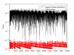
(a) $\alpha=-0.5$.

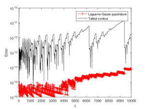
(a) $\alpha=0.5$.

Fig. 1: Comparison between the trapezoidal rule based on the Talbot contour (black curve) and the LG quadrature (red curve), $\tau=1$, $B=5,N=100$. The optimal contour $z(\theta,t)=t\left(-0.4814+0.6443(\theta\cot(\theta)+i0.5653\theta)\right)$ obtained in [37] is applied here, i.e., $\hat{\lambda}_{j}^{(\ell)}$ in (13) is given by $\hat{\lambda}_{j}^{(\ell)}=z(\theta_{j},N/(2T_{\ell}-\tau))$ with the corresponding weight $\hat{\omega}_{j}^{(\ell)}=\partial_{\theta}z(\theta_{j},N/(2T_{\ell}-\tau))$, where $\theta_{j}=(2j+1)\pi/(2N),j=-N,...,N-1$ and $T_{\ell}=B^{\ell}\tau$, $B=5,N=32$.

3 Short memory principle with lag terms

In this section, we generalize the fast convolution in the previous section to resolve the short memory principle (see [6, 29]). The error analysis of the method is given in the next section.

Let ${\Delta T}\geq 0$ be a memory length. Divide the convolution $k_{\alpha}*u(t)$ into the local part $L^{\alpha}_{{\Delta}T}(u,t)$ and the history part $H^{\alpha}_{{\Delta}T}(u,t)$ as shown below

(16) $$k_{\alpha}*u(t) \equiv L^{\alpha}_{{\Delta}T}(u,t)+H^{\alpha}_{{\Delta}T}(u,t),$$

(17) $$L^{\alpha}_{{\Delta}T}(u,t) = \int_{\max\{0,t-{\Delta}T\}}^{t}k_{\alpha}(t-s)u(s)\,{\rm d}s,$$

(18) $$H^{\alpha}_{{\Delta}T}(u,t) = \int_{0}^{\max\{0,t-{\Delta}T\}}k_{\alpha}(t-s)u(s)\,{\rm d}s.$$

If we drop the history part in (16), then the remaining part is the famous short memory principle rule (see [29]). However, the short memory principle has not been widely applied, since $L^{\alpha}_{{\Delta}T}(u,t)$ is not a good approximation of $k_{\alpha}*u(t)$. Our goal is to develop a good numerical approximation of $H^{\alpha}_{{\Delta}T}(u,t)$, such that the storage and computational cost are reduced significantly compared with the direct approximation. The local part $L^{\alpha}_{{\Delta}T}(u,t)$ is just the fractional operator defined on $[\max\{0,t-{\Delta}T\},t]$, which can be discretized directly by the known methods, see [11, 21, 24, 34]. Next, we introduce how to discretize (16) efficiently and accurately.

3.1 Interpolations

In this work, the discretization of (17) and (18) is based on the interpolation of $u$. Specifically, $L^{\alpha}_{{\Delta}T}(u,t)$ and $H^{\alpha}_{{\Delta}T}(u,t)$ are approximated by $L^{\alpha}_{{\Delta}T}(I^{L}_{\tau}u,t)$ and $H^{\alpha}_{{\Delta}T}(I^{H}_{\tau}u,t)$, respectively, where $I^{L}_{\tau}$ and $I^{H}_{\tau}$ are two suitable piecewise interpolation operators, which will be discussed in the following.

Linear interpolation is simple and has been applied widely in the discretization of the fractional operators, see [8, 15, 17, 34]. Several quadratic interpolations have been used to discretize the Caputo fractional operators, see, for example, [40, 19, 24]. We adopt the quadratic interpolation in [24] to illustrate the implementation of the present fast algorithm. Define the local interpolation operator $\Pi^{j}_{\tau}$ as

(19) $$\Pi^{j}_{\tau}u(t)=\sum_{k=1}^{3}u_{j+k-1}F_{k}^{(j)}(t),{\quad}t\in[t_{j},t_{j+1}],j\geq 0,$$

where $F^{(j)}_{1}=\frac{(t-t_{j+1})(t-t_{j+2})}{(t_{j}-t_{j+1})(t_{j}-t_{j+2})}$, $F^{(j)}_{2}=\frac{(t-t_{j})(t-t_{j+2})}{(t_{j+1}-t_{j})(t_{j+1}-t_{j+2})}$, and $F^{(j)}_{3}=\frac{(t-t_{j})(t-t_{j+1})}{(t_{j+2}-t_{j})(t_{j+2}-t_{j+1})}$. Let $\Pi^{-1}_{\tau}u(t)=\Pi^{0}_{\tau}u(t)$. Then, for each $n\geq 1$, the quadratic interpolation $I^{(2,n)}_{\tau}$ is defined by

(20) $$I^{(2,n)}_{\tau}u(t)=\left\{\begin{aligned} &\Pi^{j}_{\tau}u(t),\quad t\in[t_{j},t_{j+1}],0\leq j\leq n-2,\\ &\Pi^{n-2}_{\tau}u(t),{\quad}t\in[t_{n-1},t_{n}].\end{aligned}\right.$$

For each $n\geq 1$, we define $I^{L}_{\tau}$ and $I^{H}_{\tau}$ as follows

(21) $$I^{L}_{\tau}u(t) = I^{(2,n)}_{\tau}u(t),{\qquad}t\in[\max\{t_{n}-\Delta T,0\},t_{n}],$$

(22) $$I^{H}_{\tau}u(t) = I^{(2,n)}_{\tau}u(t),{\qquad}t\in[0,\max\{t_{n}-\Delta T,0\}].$$

Let $j_{n}=\max\{n-n_{0},0\}$. Then $L^{(\alpha,n)}_{\Delta T,\tau}u=L^{\alpha}_{{\Delta}T}(I^{L}_{\tau}u,t_{n})$ and $H^{(\alpha,n)}_{\Delta T,\tau}u=H^{\alpha}_{{\Delta}T}(I^{H}_{\tau}u,t_{n})$ are given by

(23) $$L^{(\alpha,n)}_{\Delta T,\tau}u = \sum_{j=j_{n}}^{n-2}\left(b^{(1)}_{n-1-j}u_{j}+b^{(2)}_{n-1-j}u_{j+1}+b^{(3)}_{n-1-j}u_{j+2}\right)+\sum_{j=0}^{2}d_{j}u_{n+j-2},$$

(24) $$H^{(\alpha,n)}_{\Delta T,\tau}u = \sum_{j=0}^{j_{n}-1}\left(b^{(1)}_{n-1-j}u_{j}+b^{(2)}_{n-1-j}u_{j+1}+b^{(3)}_{n-1-j}u_{j+2}\right),$$

where $b_{n-j-1}^{(k)}=\int_{t_{j}}^{t_{j+1}}k_{\alpha}(t_{n}-s)F^{(j)}_{k}(s)\,{\rm d}s$ and $d_{j}=\int_{t_{n-1}}^{t_{n}}k_{\alpha}(t_{n}-s)F^{(n-2)}_{j}(s)\,{\rm d}s$, i.e.,

(25) $$d_{0} = \frac{-\alpha\tau^{\alpha}}{2\Gamma(\alpha+3)},{\quad}d_{1}=\frac{\alpha(3+\alpha)\tau^{\alpha}}{\Gamma(\alpha+3)},{\quad}d_{2}=\frac{(4+\alpha)\tau^{\alpha}}{2\Gamma(\alpha+3)},$$

(26) $$b^{(1)}_{j} = \frac{\tau^{\alpha}}{2\Gamma(\alpha)}\left[\ell_{j}^{(\alpha+2)}-(2j-1)\ell_{j}^{(\alpha+1)}+j(j-1)\ell_{j}^{(\alpha)}\right],$$

(27) $$b^{(2)}_{j} = -\frac{\tau^{\alpha}}{\Gamma(\alpha)}\left[\ell_{j}^{(\alpha+2)}-2j\ell_{j}^{(\alpha+1)}+(j+1)(j-1)\ell_{j}^{(\alpha)}\right],$$

(28) $$b^{(3)}_{j} = \frac{\tau^{\alpha}}{2\Gamma(\alpha)}\left[\ell_{j}^{(\alpha+2)}-(2j+1)\ell_{j}^{(\alpha+1)}+j(j+1)\ell_{j}^{(\alpha)}\right],$$

(29) $$\ell_{j}^{(\alpha)} = \frac{1}{\alpha}\left[(j+1)^{\alpha}-j^{\alpha}\right].$$

Some researchers used other interpolations in the discretization of the fractional integral and derivative operators, we refer readers to [19, 7, 8, 17, 10, 42].

3.2 Corrections

From (23)–(24) and for any $\Delta T\geq 0$, we always have

(30) $$D^{(\alpha,n)}_{\Delta T,\tau}u=L^{(\alpha,n)}_{\Delta T,\tau}u+H^{(\alpha,n)}_{\Delta T,\tau}u=\sum_{j=0}^{n}w_{n,j}u_{j},$$

where $w_{n,j}$ can be derived from (25)–(28), which do not give explicitly. Clearly, $D^{(\alpha,n)}_{\Delta T,\tau}u$ is just the second-order trapezoidal rule (or the $(2+\alpha)$-order L1 method) for the fractional integral of order $\alpha>0$ (or the RL fractional derivative of order $0<-\alpha<1$) if the linear interpolation is used and $u(t)$ is sufficiently smooth, see [7, 8]. For quadratic interpolation (LABEL:quadratic), $D^{(\alpha,n)}_{\Delta T,\tau}u$ achieves the $(3+\alpha)$-order accuracy for the RL derivative of order $0<-\alpha<1$ when $u(t)$ is smooth. However, the approximation $D^{(\alpha,n)}_{\Delta T,\tau}u$ defined by (30) is not a good approximation of $k_{\alpha}*u(t_{n})$ when $u(t)$ has strong singularities.

In this work, we follow Lubich’s idea (see [21]) to use correction terms to capture the singularity of the solution $u(t)$ to the considered FODE. The correction method is based on the assumption that the solution $u(t)$ has the following form

(31) $$u(t)-u(0)=\sum_{j=1}^{m}c_{j}t^{\sigma_{j}}+t^{\sigma_{m+1}}\tilde{u}(t),{\quad}0<\sigma_{j}<\sigma_{j+1},$$

where $\tilde{u}(t)$ is uniformly bounded for $t\in[0,T]$. Readers can refer to [8, 23, 13, 29] for more detailed results of the regularity of FODEs.

Combining (30) and (31) gives the following correction method

(32) $$D^{(\alpha,n,m)}_{\Delta T,\tau}u = D^{(\alpha,n)}_{\Delta T,\tau}u+\tau^{\alpha}\sum_{j=1}^{m}W_{n,j}(u_{j}-u_{0}),$$

where $W_{n,j}$ are the starting weights that are chosen such that

(33) $$D^{(\alpha,n)}_{\Delta T,\tau}u+\tau^{\alpha}\sum_{j=1}^{m}W_{n,j}(u_{j}-u_{0})=k_{\alpha}*u(t_{n})=\frac{\tau^{\alpha}n^{\sigma_{k}+\alpha}}{\Gamma(\sigma_{k}+1+\alpha)},1\leq k\leq m$$

for $u(t)=t^{\sigma_{k}},0<\sigma_{k}<\sigma_{k+1}$. For each $n>0$, one can resolve $W_{n,j}(1\leq j\leq m)$ from the above linear system and $W_{n,j}$ are independent of $\tau$. The error analysis of the direct method (32) is discussed in Section 4. Readers can refer to [9, 21, 44] for more discussions of the correction method.

3.3 The fast implementation

In this subsection, we generalize the fast algorithm in Section 2 to approximate $D^{(\alpha,n)}_{\Delta T,\tau}$ defined by (30), which is given as follows.

• Step A) Decompose $D^{(\alpha,n)}_{\Delta T,\tau}u$ into two parts as $D^{(\alpha,n)}_{\Delta T,\tau}u=L^{(\alpha,n)}_{\Delta T,\tau}u+H^{(\alpha,n)}_{\Delta T,\tau}u$.

• Step B) Assume that ${{\Delta}T}=n_{0}\tau=t_{n_{0}}$. For every $t=t_{n},n\geq n_{0}$, let $L$ be the smallest integer satisfying $t_{n-n_{0}+1}<2B^{L}\tau$. For $\ell=1,2,...,L-1$, determine the integer $q_{\ell}$ such that

  (34) $$s_{\ell}=q_{\ell}B^{\ell}\tau\quad\text{satisfies}\quad t_{n-n_{0}+1}-s_{\ell}\in[B^{\ell}\tau,(2B^{\ell}-1)\tau].$$

  Set $s_{0}=t_{n-n_{0}+1}-\tau$ and $s_{L}=0$.

• Step C) Let $\hat{t}_{n}=t_{n}-{{\Delta}T}+\tau=t_{n-n_{0}+1}\geq\tau$. Then the history part $H^{(\alpha,n)}_{{\Delta}T,\tau}u=H^{\alpha}_{{\Delta}T}(I^{H}_{\tau}u,t_{n})$ is approximated by

  (35) $$H^{(\alpha,n)}_{{\Delta}T,\tau}u = \frac{\sin(\alpha\pi)}{\pi}\sum_{\ell=1}^{L}\int_{0}^{\infty}\lambda^{-\alpha}e^{-(T_{\ell-1}+{{\Delta}T}-\tau)\lambda}e^{-(\hat{t}_{n}-s_{\ell-1}-T_{\ell-1})\lambda}y(s_{\ell-1},s_{\ell},\lambda)\,{\rm d}\lambda$$

  $$\approx \frac{\sin(\alpha\pi)}{\pi}\sum_{\ell=1}^{L}\sum_{j=0}^{{q}_{\alpha}{(N_{\ell})}}\omega_{j}^{(\ell)}e^{-(\hat{t}_{n}-s_{\ell-1}-T_{\ell-1}){\lambda}^{(\ell)}_{j}}y(s_{\ell-1},s_{\ell},\lambda^{(\ell)}_{j}):={}_{F}H_{\Delta T,\tau}^{(\alpha,n)}u,$$

  where $\{\omega^{(\ell)}_{j}\}$ and $\{\lambda^{(\ell)}_{j}\}$ are the LG quadrature weights and points that correspond to the weight function $\lambda^{-\alpha}e^{-(T_{\ell-1}+{{\Delta}T}-\tau)\lambda}$, ${q}_{\alpha}{(N_{\ell})}$ is defined by (44), and $y(s_{\ell-1},s_{\ell},\lambda^{(\ell)}_{j})$ can be be obtained exactly by solving the following linear ODE

  (36) $$y^{\prime}(s)=-\lambda^{(\ell)}_{j}y(s)+I^{H}_{\tau}u(s),{\quad}y(s_{\ell})=0,$$

  see also (10) and (11).

• Step D) Calculate the local part $L^{(\alpha,n)}_{\Delta T,\tau}u=L^{\alpha}_{{\Delta}T}(I^{L}_{\tau}u,t_{n})$.

The fast algorithm for the discretization of $k_{\alpha}*u(t)$ is now given by

(37) $${}_{F}D^{(\alpha,n,m)}_{\Delta T,\tau}u=L^{(\alpha,n)}_{\Delta T,\tau}u+{}_{F}H^{(\alpha,n)}_{\Delta T,\tau}u+\tau^{\alpha}\sum_{j=1}^{m}W_{n,j}(u_{j}-u_{0}),$$

where $L^{(\alpha,n)}_{\Delta T,\tau}$ is given by (23), ${}_{F}H^{(\alpha,n)}_{\Delta T,\tau}u$ is given by (35), and the starting weights $W_{n,j}$ are determined by the linear system (33).

Next, we analyze the complexity of the present fast method (37). For the local part $L^{(\alpha,n)}_{\Delta T,\tau}u$, the memory requirement is $O(n_{0})$ with the computational cost of $O(n_{0}(n_{T}-n_{0}))$ for all $n_{0}<n\leq n_{T}$. For the history part ${}_{F}H^{(\alpha,n)}_{\Delta T,\tau}u$, we have $O(\sum_{\ell}^{L}{q}_{\alpha}(N_{\ell}))$ active memory and $O((n_{T}-n_{0})\sum_{\ell}^{L}{q}_{\alpha}(N_{\ell}))$ operations, where $L=\log_{B}{(n_{T}-n_{0})}$. An additional cost is required to obtain the starting weights $W_{n,j}$ in (37), which can be performed by use of fast Fourier transform with $O(n_{T}\log(n_{T}))$ arithmetic operations. Hence, the overall active memory and computational cost are $O(n_{0}+\sum_{\ell}^{L}{q}_{\alpha}(N_{\ell}))$ and $O(n_{0}n_{T}+(n_{T}-n_{0})\sum_{\ell}^{L}{q}_{\alpha}(N_{\ell}))$, respectively.

4 Error analysis

In this section, we analyse the overall discretization error of the fast method (37) in Section 3. Firstly, we present the exponential convergence rate of the LG quadrature used in (8) and (35). Then we show how to choose $N_{\ell}$ and ${q}_{\alpha}(N_{\ell})$ used in (35), such that the desired accuracy is maintained with the use of the minimum number of the quadrature points.

For simplicity, we denote

(38) $$I^{\alpha}[T,f]=\int_{0}^{\infty}\lambda^{\alpha}e^{-T\lambda}f(\lambda)\,{\rm d}\lambda{\quad}\text{and}{\quad}I^{\alpha}[f]=\int_{0}^{\infty}\lambda^{\alpha}e^{-\lambda}f(\lambda)\,{\rm d}\lambda.$$

The LG quadrature for $I^{\alpha}[T,f]$ and $I^{\alpha}[f]$ are given by (see [32])

(39) $$Q_{N}^{\alpha}[T,f]=T^{-\alpha-1}\sum_{j=0}^{N}{w}^{(\alpha)}_{j}f({\lambda}_{j}/T),{\quad}Q_{N}^{\alpha}[f]=\sum_{j=0}^{N}{w}^{(\alpha)}_{j}f({\lambda}_{j}),$$

where $\lambda_{j}$ are the roots of the Laguerre polynomial $L_{N+1}^{(\alpha)}({\lambda})$, and ${w}^{(\alpha)}_{j}$ are the corresponding weights given by

(40) $${w}^{(\alpha)}_{j}=\frac{\Gamma(N+\alpha+1){\lambda}_{j}}{(N+\alpha+1)(N+1)!}\big{(}L_{N}^{(\alpha)}({\lambda}_{j})\big{)}^{-2}.$$

We show the convergence of the quadrature $Q_{N}^{\alpha}[T,e^{-t\lambda}]$ and the property of the quadrature weight ${w}^{(\alpha)}_{j}$ (see (40)) in the following two theorems. The proofs are given in Appendix A.

Theorem 1.

Let $t\geq 0,T>0$, $\alpha>-1$, and $N$ be sufficiently large. Then

(41) $$\left|I^{\alpha}[T,e^{-t\lambda}]-Q_{N}^{\alpha}[T,e^{-t\lambda}]\right|\leq C_{\alpha,N}T^{-\alpha-1}\left(\frac{t/T}{1+t/T}\right)^{2N},$$

where $C_{\alpha,N}$ is bounded $-1<\alpha\leq 0$ and $C_{\alpha,N}\leq C_{\alpha}N^{\alpha}$ for $\alpha>0$.

Theorem 2.

Let $\alpha>-1$ and $w^{(\alpha)}_{j}$ be defined by (40). If $N$ and $j$ are sufficiently large, then there exists a positive constant $C$ independent of $N$ such that

(42) $${w}^{(\alpha)}_{j}\leq C(N+1)^{\alpha}e^{-0.25\pi^{2}(j+1)^{2}/(N+1)}.$$

Given a precision $\epsilon_{0}>0$, the truncated LG quadrature is given by

(43) $$Q_{N,\epsilon_{0}}^{\alpha}[T,f]=T^{-\alpha-1}\sum_{j=0}^{q_{-\alpha}(N)}{w}^{(\alpha)}_{j}f({\lambda}_{j}/T),$$

where $q_{-\alpha}(N)$ is a positive number given by

(44) $$q_{-\alpha}(N)=\min\Big{\{}N,\left\lceil{2}{\pi^{-1}}\sqrt{(N+1)\log((N+1)^{\alpha}\epsilon^{-1}_{0})}\right\rceil-1\Big{\}}.$$

From (42), we can find the smallest integer $j$ satisfying $(N+1)^{\alpha}e^{-0.25\pi^{2}(j+1)^{2}/(N+1)}\leq\epsilon_{0}$, which yields (44). We choose $\epsilon_{0}=10^{-16}$ in this paper.

Figure 2 (a) shows the exponential decay of ${w}^{(-\alpha)}_{j}$ when $j\geq{q}_{\alpha}(128)$ for different fractional orders $\alpha=-1.8,-1.2,-0.8,-0.2,0.2,0.8$. Figure 2 (b) displays similar behaviors as shown in Figure 2 (a). We can see that Eq. (44) works well, and ${q}_{\alpha}(N)$ is not very sensitive to the fractional order $\alpha\in(-2,1)$. For example, ${q}_{\alpha}(128)=(48,47,46,44,43,41)$ (or ${q}_{\alpha}(256)=(69,67,65,62,61,58)$) for $\alpha=(-1.8,-1.2,-0.8,-0.2,0.2,0.8)$, and ${q}_{\alpha}(N)\ll N$ when $N$ is sufficiently large. For $\alpha\leq-2$, similar results are obtained, which is not shown here.

(a) $N=128$.

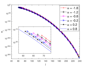
(b) $N=256$.

Fig. 2: The exponential decay of the quadrature weights ${w}^{(-\alpha)}_{j}$ defined by (40).

For notational simplicity, we denote

$$\widehat{T}_{\ell}=T_{\ell-1}+{\Delta}T-\tau,{\quad}\widehat{H}^{n}_{\ell}(s)=\hat{t}_{n}-T_{\ell-1}-s.$$

Next, we investigate how to estimate $N_{\ell}$ in (35), such that the LG quadrature $Q_{N_{\ell}}^{-\alpha}[\widehat{T}_{\ell},e^{-\widehat{H}^{n}_{\ell}(s)\lambda}]$ to the integral $I^{-\alpha}[\widehat{T}_{\ell},e^{-\widehat{H}^{n}_{\ell}(s)\lambda}]$ preserves the accuracy up to $O(\epsilon)$ for all $s\in[s_{\ell},s_{\ell-1}]$.

From Theorem 1, we know that the error of $Q_{N_{\ell}}^{-\alpha}[\widehat{T}_{\ell},e^{-\widehat{H}^{n}_{\ell}(s)\lambda}]$ mainly depends on the following term

$$\left({\widehat{H}^{n}_{\ell}(s)}/{\widehat{T}_{\ell}}\right)^{2N}=\left(\frac{\hat{t}_{n}-s-T_{\ell-1}}{T_{\ell-1}+{\Delta}T-\tau}\right)^{2N},\quad s\in[s_{\ell},s_{\ell-1}].$$

Using (34) and $T_{\ell-1}=B^{\ell-1}\tau$ gives

(45) $$0\leq\frac{\hat{t}_{n}-s-T_{\ell-1}}{T_{\ell-1}+{\Delta}T-\tau}\leq\frac{2B-1-B^{1-\ell}}{1+B^{1-\ell}({\Delta}T/\tau-1)}=\mathcal{T}_{\ell}\leq 2B-1,{\quad}\forall\ell\geq 1.$$

Using the above inequality and Eq. (41) yields

(46) $$\big{|}I^{-\alpha}[\widehat{T}_{\ell},e^{-\widehat{H}^{n}_{\ell}(s)\lambda}]-Q_{N_{\ell}}^{-\alpha}[\widehat{T}_{\ell},e^{-\widehat{H}^{n}_{\ell}(s)\lambda}]\big{|}$$

$$\leq C_{\alpha,N_{\ell}}\widehat{T}_{\ell}^{\alpha-1}\left(\frac{{\widehat{H}^{n}_{\ell}(s)}/{\widehat{T}_{\ell}}}{1+{\widehat{H}^{n}_{\ell}(s)}/{\widehat{T}_{\ell}}}\right)^{2N_{\ell}}\leq C_{\alpha,N_{\ell}}\widehat{T}_{\ell}^{\alpha-1}\left(\frac{\mathcal{T}_{\ell}}{1+\mathcal{T}_{\ell}}\right)^{2N_{\ell}}.$$

Since the relative error of (46) is independent of $\widehat{T}_{\ell}$, we can let $(\mathcal{T}_{\ell}/(\mathcal{T}_{\ell}+1))^{2N_{\ell}}\leq\epsilon$, which yields the minimum $N_{\ell}$ given by

(47) $$N_{\ell}=\left\lceil\frac{\log\epsilon}{2\log(\frac{\mathcal{T}_{\ell}}{\mathcal{T}_{\ell}+1})}\right\rceil,\quad\mathcal{T}_{\ell}=\frac{2B-1-B^{1-\ell}}{1+B^{1-\ell}({\Delta}T/\tau-1)}.$$

From (43) and (46), we derive that the pointwise error of the truncated quadrature $Q_{N_{\ell},\epsilon_{0}}^{-\alpha}[\widehat{T}_{\ell},e^{-\widehat{H}^{n}_{\ell}(s)\lambda}]$ for all $s\in[s_{\ell},s_{\ell-1}]$ is given by

(48) $$E^{-\alpha,\ell}_{\epsilon,\epsilon_{0}}[e^{-\widehat{H}^{n}_{\ell}(s)\lambda}]=I^{-\alpha}[\widehat{T}_{\ell},e^{-\widehat{H}^{n}_{\ell}(s)\lambda}]-Q_{N_{\ell},\epsilon_{0}}^{-\alpha}[\widehat{T}_{\ell},e^{-\widehat{H}^{n}_{\ell}(s)\lambda}]=O(\epsilon)+O(\epsilon_{0}),$$

where $Q_{N_{\ell},\epsilon_{0}}^{-\alpha}$ is defined by (43) and $N_{\ell}$ is given by (47).

Next, we present the error bound of the fast method in Section 3. Denote by

(49) $$R^{(n)}=\int_{0}^{t_{n}}k_{\alpha}(t_{n}-s)u(s)\,{\rm d}s-D^{(\alpha,n,m)}_{\Delta T,\tau}u.$$

Note that the above discretization error $R^{(n)}$ depends on the smoothness of $u(t)$ and the discretization method $D^{(\alpha,n,m)}_{\Delta T,\tau}u$. If $u(t)$ is sufficiently smooth, no correction terms are needed to achieve $(2+\alpha)$-order (or $(3+\alpha)$-order) accuracy if linear (or quadratic) interpolation is applied for $\alpha<0$. If $u(t)$ satisfies (31), then the global $(2+\alpha)$-order (or $(3+\alpha)$-order) accuracy can be achieved for $\sigma_{m+1}\geq 2$ (or $\sigma_{m+1}\geq 3$). In numerical simulations, the condition $\sigma_{m+1}\geq 2$ (or $\sigma_{m+1}\geq 3$) does not need to be satisfied, $(2+\alpha)$-order (or $(3+\alpha)$-order) accurate numerical solutions are observed far from $t=0$. In the numerical simulations, only a small number of correction terms are sufficient to achieve very accurate numerical solutions; see numerical simulations in the following section and see also related results in [44].

From (35) and (48), we have

(50) $$\big{|}H^{\alpha}_{{\Delta}T} (I^{H}_{\tau}u,t_{n})-{}_{F}H_{\Delta T,\tau}^{(\alpha,n)}u\big{|}=\Big{|}\frac{\sin(\alpha\pi)}{\pi}\sum_{\ell=1}^{L}E^{-\alpha,\ell}_{\epsilon,\epsilon_{0}}[e^{-(\hat{t}_{n}-T_{\ell-1}-s_{\ell-1})\lambda}y(s_{\ell-1},s_{\ell},\lambda)]\Big{|}$$

$$= \Big{|}\frac{\sin(\alpha\pi)}{\pi}\sum_{\ell=1}^{L}\int_{s_{\ell}}^{s_{\ell-1}}E^{-\alpha,\ell}_{\epsilon,\epsilon_{0}}[e^{-\widehat{H}^{n}_{\ell}(s)\lambda}]I_{\tau}^{H}u(s)\,{\rm d}s\Big{|}$$

$$\leq C(\epsilon+\epsilon_{0})\int_{0}^{\hat{t}_{n}}\big{|}I_{\tau}^{H}u(s)\big{|}\,{\rm d}s\leq C\max\{0,t_{n+1}-\Delta T\}\|u\|_{\infty}(\epsilon+\epsilon_{0}).$$

Combining (49) and (50) yields

(51) $$\Big{|}k_{\alpha}*u(t_{n})-{}_{F}D_{\Delta T,\tau}^{(\alpha,n,m)}u\Big{|}= \Big{|}H^{\alpha}_{{\Delta}T}(I^{H}_{\tau}u,t_{n})-{}_{F}H_{\Delta T,\tau}^{(\alpha,n)}u+R^{(n)}\Big{|}$$

$$\leq C\max\{0,t_{n+1}-\Delta T\}\|u\|_{\infty}(\epsilon+\epsilon_{0})+\big{|}R^{(n)}\big{|},$$

where the error in (51) originates from two parts: the LG quadrature for discretizing $I^{-\alpha}[\widehat{T}_{\ell},e^{-\widehat{H}^{n}_{\ell}(s)\lambda}]$ (see (48)) and the discretization error defined by (49).

Next, we numerically study the error caused by the LG quadrature. Let $m=0$ and $u(t)=1+t$. Then $R^{(n)}$ in (51) is zero. Denote the relative pointwise error

$$e_{n}=\left(k_{\alpha}*u(t_{n})\right)^{-1}\Big{|}k_{\alpha}*u(t_{n})-{}_{F}D_{\Delta T,\tau}^{(\alpha,n,0)}u\Big{|},{\quad}1\leq n\leq n_{T}=T/\tau,$$

where $k_{\alpha}*u(t_{n})=t_{n}^{\alpha}/\Gamma(1+\alpha)+t_{n}^{\alpha+1}/\Gamma(2+\alpha)$ for $u(t)=1+t$.

Given a precision $\epsilon=10^{-10}$, the maximum relative error $\|e\|_{\infty}=\max_{0\leq n\leq n_{T}}\big{|}e_{n}\big{|}$, the total number of the quadrature points $\sum{N_{\ell}}$, and the total number of the truncated quadrature points $\sum{q}_{\alpha}(N_{\ell})$ are shown in Table 1 for different basis $B$, $\alpha=-0.5,\tau=0.1,{\Delta}T=1$, and $T=10^{4}$. We can see that the truncated LG quadrature saves memory. A relatively smaller basis $B$ needs less quadrature points and thus saves memory, which can be explained from (45) and (46). Eq. (46) implies a faster convergence as $B$ decreases, due to $T_{\ell}\approx 2B-1$, $\ell$ is sufficiently large. Hence, a relatively smaller $B$ means that smaller $N_{\ell}$ are needed to achieve high accuracy that leads to the use of less LG quadrature points.

We change the precision $\epsilon$ and show the corresponding relative maximum errors $\|e\|_{\infty}$ in Table 2. We can see that $\|e\|_{\infty}$ increases as $\epsilon$ increases and the total number of the quadrature points are reduced. It also shows that much better results are obtained than the theoretical prediction, see also the related results in Table 7.

Table 1: The maximum relative error $\|e\|_{\infty}$ under the precision $\epsilon=10^{-10}$, $\alpha=-0.5,\tau=0.1,{\Delta}T=1$, and $T=10^{4}$.

$B$	$\sum N_{\ell}$	$\sum{q}_{\alpha}(N_{\ell})$	$\|e\|_{\infty}$	$B$	$\sum N_{\ell}$	$\sum{q}_{\alpha}(N_{\ell})$	$\|e\|_{\infty}$
2	583	389	6.8651e-13	30	3333	545	7.2134e-13
3	605	323	6.6718e-13	40	3583	514	7.3190e-13
4	687	318	7.4246e-13	50	4521	576	7.3391e-13
5	783	320	7.4754e-13	60	5463	637	7.4632e-13
8	1151	370	7.4377e-13	70	6406	689	7.3451e-13
10	1246	359	7.1388e-13	80	7345	737	7.4678e-13
15	1598	376	6.9954e-13	90	8288	785	7.3892e-13
20	2173	438	7.0761e-13	100	9231	829	7.4941e-13

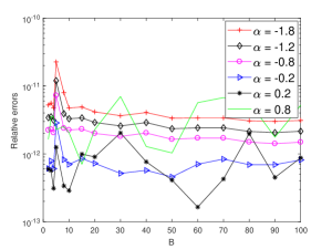
(a)

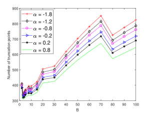
(b)

Fig. 3: (a) The maximum relative error $\|e\|_{\infty}$ against the basis $B$; (b) The total number $\sum{q}_{\alpha}(N_{\ell})$ of the quadrature points against $B$; $\tau=0.01,T=10^{4},\epsilon=10^{-10}$.

Figure 3 (a) shows the relative maximum error $\|e\|_{\infty}$ against the basis $B$ for different fractional orders, $\tau=0.01,T=10^{4},\epsilon=10^{-10}$. We can see that better results are obtained than the predicted precision $\epsilon=10^{-10}$, even for $\alpha=-1.8$ (the fractional derivative of order $1.8$). Figure 3 (b) shows the total number of the truncated LG quadrature points against the basis $B$. For a fixed $B$, the number of truncated quadrature points increases as $\alpha$ decreases, which is in line with the theoretical prediction (44). For a fixed fractional order $\alpha$, the number of the truncated quadrature points increases as $B$ increases, which agrees with (47), due to $\mathcal{T}_{\ell}\approx 2B-1$ when $\ell$ is sufficiently large.

It is reasonable to choose a relatively smaller precision $\epsilon$ and smaller basis $B$ in numerical simulations, since a smaller $\epsilon$ ensures a relatively large $N_{\ell}$ that guarantees the exponential convergence of the LG quadrature, and a small $B$ ensures a smaller radius of convergence of the quadrature error (46).

Table 2: The maximum relative error $\|e\|_{\infty}$ under different precision $\epsilon$, $B=5$, $\alpha=-0.5,{\Delta}T=1$.

	$\tau=0.01,T=10^{4}$			$\tau=0.1,T=10^{5}$
$\epsilon$	$\sum N_{\ell}$	$\sum{q}_{\alpha}(N_{\ell})$	$\|e\|_{\infty}$	$\sum N_{\ell}$	$\sum{q}_{\alpha}(N_{\ell})$	$\|e\|_{\infty}$
$10^{-12}$	1018	384	1.1937e-12	1203	442	6.8208e-12
$10^{-10}$	848	349	4.7044e-12	1001	402	6.8191e-12
$10^{-8}$	680	313	4.7044e-12	799	361	6.5369e-12
$10^{-6}$	512	271	3.1858e-09	604	312	1.2450e-10
$10^{-5}$	427	243	2.1577e-06	503	281	1.8889e-08
$10^{-4}$	340	215	2.1577e-06	404	252	2.3317e-07

Finally in this section, we compare the truncated LG quadrature with the multipole approximation proposed in [2]. As the key idea of the existing fast methods aforementioned is to seek a sum-of-exponentials of the form $\sum\omega_{j}e^{-\lambda_{j}t}$ to approximate the kernel function $k_{\alpha}(t)$, we compare the accuracy of the sum-of-exponentials from the LG quadrature and the multipole approximation. The relative pointwise errors $e_{n}=\big{|}k_{\alpha}(t_{n})-\sum\omega_{j}e^{-\lambda_{j}t_{n}}\big{|}/\big{|}k_{\alpha}(t_{n})\big{|}$ are shown in Figure 4, where we set the precision $\epsilon=10^{-10}$, $B=5$, and $\Delta T=\tau$ when the LG quadrature is applied, and the precision in [2] is set to be $10^{-14}$. For $\alpha=0.5$, the two methods achieve similar accuracy with, respectively, $P=832$ and $Q=777$ quadrature points for the multipole approximation and the truncated LG quadrature, see Figure 4 (a). Figure 4 (b) shows the pointwise errors for $\alpha=-0.5$, the truncated LG quadrature shows a slightly better approximation. For other fractional orders $\alpha\in(-1,1)$, the truncated LG quadrature is competitive with the multipole approximation both in accuracy and the computational cost. These results are not shown here.

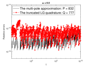
(a) $\alpha=0.5,\tau=0.0001$.

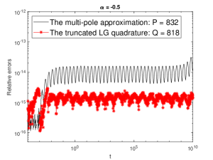
(b) $\alpha=-0.5,\tau=0.0001$.

Fig. 4: Comparison of the truncated LG quadrature and the multipole approximation [2].

5 Numerical examples and applications

In this section, two examples are presented to verify the effectiveness of the present fast method when it is applied to solve FDEs. All the algorithms are implemented using MATLAB 2016a, which were run in a 3.40 GHz PC having 16GB RAM and Windows 7 operating system.

Example 5.1.

Consider the following scaler FDE

(52) $${}_{C}D^{\alpha}_{0,t}u(t)=-Au(t)+F(u,t),{\quad}u(0)=u_{0},{\quad}t\in(0,T],$$

where $0<\alpha\leq 1$ and $A\geq 0$, and ${}_{C}D^{\alpha}_{0,t}$ is the Caputo fractional operator, which satisfies ${}_{C}D^{\alpha}_{0,t}u(t)=k_{\alpha}*u(t)-{u(0)t^{-\alpha}}/{\Gamma(1-\alpha)}$, see [29].

We present our fast numerical method for (52) as follows: For a given length $\Delta T=n_{0}\tau$, find $U_{n}$ for $n>n_{0}$ such that

(53) $${}_{F}D^{(-\alpha,n,m)}_{\Delta T,\tau}U-{u_{0}t_{n}^{-\alpha}}/{\Gamma(1-\alpha)}=-AU_{n}+F(U_{n},t_{n}),$$

where ${}_{F}D^{(\alpha,n,m)}_{\Delta T,\tau}$ is defined by (37). The application of the direct convolution method means here that ${}_{F}D^{(-\alpha,n,m)}_{\Delta T,\tau}U$ in (53) is replaced by $D^{(-\alpha,n,m)}_{\Delta T,\tau}U$. The Newton method is used to solve the nonlinear system (53). The direct method is applied to obtain $U_{k}(\leq k\leq m)$, and the stating values $U_{k}(1\leq k\leq m)$ are obtained using the direct method with one correction term and a smaller stepsize $\tau^{-2}$.

The following two cases are considered in this example.

• Case I: For the linear case of $F=0$, the exact solution of (52) is

  $$u(t)=E_{\alpha}(-At^{\alpha}),$$

  where $E_{\alpha}(t)$ is the Mittag–Leffler function defined by $E_{\alpha}(t)=\sum_{k=0}^{\infty}\frac{t^{k}}{\Gamma(k\alpha+1)}.$

• Case II: Let $F=u(1-u^{2})$ and the initial condition is taken as $u_{0}=1$.

The maximum error is defined by

$$\|e\|_{\infty}=\max_{0\leq n\leq{T}/\tau}\big{|}e_{n}\big{|},{\quad}e_{n}=u(t_{n})-U_{n},T=40.$$

In this example, we always choose the memory length ${\Delta T}=0.5$, the basis $B=5$, the truncation number ${q}_{\alpha}{(N_{\ell})}$ in (35) is calculated by (44) and $N_{\ell}$ is determined by (47) under the precision $\epsilon=10^{-10}$, and $A=1$. We will reset these parameters if needed. The fast method based on quadratic interpolation (LABEL:quadratic) is applied in this example if there is no further illustration.

The purpose of Case I is to check the effectiveness of the present fast method for non-smooth solutions. We demonstrate that adding correction terms improves the accuracy of the numerical solutions significantly. We first let $\alpha=0.8$, the maximum error and the error at $t=40$ are shown in Tables 3 and 4, respectively. We can see that the expected convergence rate $3-\alpha$ is almost achieved by adding two or three correction terms, and the numerical solution at the final time is much more accurate than that near the origin. This phenomenon can be observed from the existing time-stepping methods for time-fractional differential equations.

As the fractional order decreases, the singularity of the analytical solution becomes stronger. Tables 5 and 6, respectively, show the maximum errors and the errors at $t=40$ for $\alpha=0.1$. We observe that the maximum error, which occurs near the origin, almost does not improve, though the step size decreases. We find that as the number of correction terms increases, the accuracy of the numerical solutions increases significantly. We need almost 30 correction terms to derive the expected global convergence rate $3-\alpha$ for $\alpha=0.1$, which is impossible to achieve by double precision. The fact is a small number of correction terms is enough to yield satisfactory numerical solutions, which makes the present method more practical. We refer readers to [44] for more explanations and numerical results associated with this phenomenon.

Table 3: The maximum error $\|e\|_{\infty}$ of the method (53), Case I, $\sigma_{k}=k\alpha$, $\alpha=0.8$, ${T=40}$, $B=5$.

$\tau$	$m=0$	Order	$m=1$	Order	$m=2$	Order	$m=3$	Order
$2^{-5}$	2.7966e-3		1.5674e-3		3.0233e-5		3.4818e-5
$2^{-6}$	1.7545e-3	0.6726	5.4427e-4	1.5260	5.9024e-6	2.3568	7.7701e-6	2.1638
$2^{-7}$	1.0604e-3	0.7264	1.8498e-4	1.5569	1.6683e-6	1.8229	1.7199e-6	2.1756
$2^{-8}$	6.2689e-4	0.7584	6.2086e-5	1.5751	4.2485e-7	1.9733	3.7854e-7	2.1838
$2^{-9}$	3.6575e-4	0.7773	2.0686e-5	1.5856	1.0205e-7	2.0576	8.3007e-8	2.1892

Table 4: The absolute error $\left|e_{n}\right|$ of the method (53) at ${t=40}$, Case I, $\sigma_{k}=k\alpha$, $\alpha=0.8$, $B=5$.

$\tau$	$m=0$	Order	$m=1$	Order	$m=2$	Order	$m=3$	Order
$2^{-5}$	5.8890e-7		1.9977e-7		1.7531e-7		4.8407e-6
$2^{-6}$	3.0861e-7	0.9322	5.8512e-8	1.7715	3.8771e-8	2.1769	1.1237e-6	2.1069
$2^{-7}$	1.5741e-7	0.9713	1.6977e-8	1.7852	8.5112e-9	2.1875	2.5398e-7	2.1455
$2^{-8}$	7.9372e-8	0.9878	4.8985e-9	1.7931	1.8745e-9	2.1829	5.6424e-8	2.1703
$2^{-9}$	3.9821e-8	0.9951	1.4075e-9	1.7992	4.3619e-10	2.1035	1.2218e-8	2.2073

Table 5: The maximum error $\|e\|_{\infty}$ of the method (53), Case I, $\sigma_{k}=k\alpha$, $\alpha=0.1$, ${{T}=40}$, $B=5$.

$\tau$	$m=0$	Order	$m=1$	Order	$m=3$	Order	$m=5$	Order
$2^{-5}$	2.5872e-3		1.5852e-3		2.1191e-5		2.1191e-5
$2^{-6}$	2.5323e-3	0.0310	1.5017e-3	0.0781	9.6408e-6	1.1362	9.6408e-6	1.1362
$2^{-7}$	2.4750e-3	0.0330	1.4177e-3	0.0831	4.3479e-6	1.1488	4.3479e-6	1.1488
$2^{-8}$	2.4148e-3	0.0355	1.3338e-3	0.0880	1.9444e-6	1.1610	1.9444e-6	1.1610
$2^{-9}$	2.3516e-3	0.0383	1.2507e-3	0.0928	1.2279e-6	0.6631	8.6285e-7	1.1721

Table 6: The absolute error $\left|e_{n}\right|$ of the method (53) at ${t=40}$, Case I, $\sigma_{k}=k\alpha$, $\alpha=0.1$, $B=5$.

$\tau$	$m=0$	Order	$m=1$	Order	$m=3$	Order	$m=5$	Order
$2^{-5}$	6.4561e-6		6.6140e-7		1.0065e-8		4.1985e-9
$2^{-6}$	3.2045e-6	1.0106	3.1760e-7	1.0583	3.8428e-9	1.3891	1.0230e-9	2.0371
$2^{-7}$	1.5919e-6	1.0094	1.5234e-7	1.0599	1.5471e-9	1.3126	2.5282e-10	2.0166
$2^{-8}$	7.9116e-7	1.0087	7.2987e-8	1.0616	6.4397e-10	1.2645	6.4081e-11	1.9801
$2^{-9}$	3.9331e-7	1.0083	3.4930e-8	1.0632	2.7313e-10	1.2374	1.6914e-11	1.9217

Table 7 shows the difference $\eta=\max_{0\leq n\leq T/\tau}{\big{|}U_{D}^{n}-{U}_{F}^{n}\big{|}}$, where $U^{n}_{F}$ are numerical solutions derived from the fast method under the precision $\epsilon$, and $U^{n}_{D}$ are numerical solutions from the direct method. We can see that the difference $\eta$ is independent of the stepsize $\tau$, which confirms (50). Table 7 also shows that the accuracy of the present fast calculation outperforms the predicted accuracy $\epsilon$, see (50).

Table 7: The difference of the numerical solutions between the fast method and the direct method, Case I, $m=0$, $\alpha=0.1$, ${{T}=40}$, $B=5$.

$\epsilon$	$\tau=2^{-5}$	$\tau=2^{-6}$	$\tau=2^{-7}$	$\tau=2^{-8}$	$\tau=2^{-9}$
$10^{-12}$	2.8255e-13	2.7850e-13	2.7167e-13	1.1102e-15	1.4988e-15
$10^{-10}$	2.8239e-13	2.7839e-13	2.7162e-13	5.6066e-15	2.1094e-15
$10^{-8}$	2.8116e-13	3.8219e-13	6.6397e-13	2.2093e-14	8.2682e-13
$10^{-6}$	7.5677e-11	7.2366e-11	8.0116e-10	2.6198e-11	8.0352e-12
$10^{-5}$	3.2916e-11	1.9709e-10	1.2477e-10	2.6461e-10	2.2769e-10
$10^{-4}$	3.0868e-09	9.4674e-09	2.4896e-09	1.5458e-08	4.3178e-08

In Table 8, we compare the present fast method (53) based on the linear interpolation with the graded mesh method in [33], in which the nonuniform grid points are given by $t_{j}=(j\tau)^{r}$, $0\leq j\leq 1/\tau$. We can see that the fast method with correction terms is competitive with the graded mesh method for $\alpha=0.5$. In [33], the authors obtained the optimal grid mesh $t_{j}=(j\tau)^{(2-\alpha)/\alpha}$ to achieve the global $(2-\alpha)$-order accuracy, which works well when $\alpha$ is relatively large and the expected convergence rate is achieved. For the correction method, too many correction terms may harm the accuracy, but a few number of correction terms can achieve highly accurate numerical solutions, which is not investigated here, readers can refer to [9, 21, 44] for more discussion. Note that for values of $\alpha$ close to zero, the correction method is even more effective than the optimal graded mesh approach in [33].

Table 8: Comparison of the present method with the graded mesh method in [33] based on linear interpolation, Case I, $\sigma_{k}=k\alpha$, $\alpha=0.5$, $B=5$. The errors $\|e\|_{\infty}$ are displayed.

The graded mesh method [33] with grid points $t_{j}=(j\tau)^{r}$. $\tau$ $r=1$ Order $r=3/2$ Order $r=3$ Order $r=6$ Order $2^{-5}$ 3.6491e-2 1.6839e-2 2.6568e-3 2.5431e-3 $2^{-6}$ 2.7048e-2 0.4320 1.0288e-2 0.7108 1.0077e-3 1.3986 9.2945e-4 1.4521 $2^{-7}$ 1.9772e-2 0.4521 6.2162e-3 0.7268 3.7277e-4 1.4347 3.3644e-4 1.4660 $2^{-8}$ 1.4312e-2 0.4663 3.7315e-3 0.7363 1.3582e-4 1.4566 1.2096e-4 1.4759 $2^{-9}$ 1.0288e-2 0.4762 2.2313e-3 0.7419 4.9041e-5 1.4696 4.3280e-5 1.4827 The fast method based on linear interpolation with correction terms $\tau$ $m=1$ Order $m=2$ Order $m=3$ Order $m=4$ Order $2^{-5}$ 5.6366e-3 2.1893e-4 1.4976e-4 7.2351e-5 $2^{-6}$ 3.1659e-3 0.8322 1.0737e-4 1.0279 6.9115e-5 1.1156 4.4890e-5 0.6886 $2^{-7}$ 1.7231e-3 0.8777 4.9196e-5 1.1260 2.9276e-5 1.2393 2.2604e-5 0.9898 $2^{-8}$ 9.1600e-4 0.9116 2.1427e-5 1.1991 1.1719e-5 1.3208 1.0105e-5 1.1614 $2^{-9}$ 4.7862e-4 0.9364 8.9763e-6 1.2552 4.5167e-6 1.3756 4.1916e-6 1.2696

Next, we implement the present fast method for a longer time computation and compare it with the direct convolution method. We show in Figure 5(a) numerical solutions for $t\in[0,{T}],{T}=10000$, where we choose $\alpha=0.1,0.5,0.9$, and the time stepsize $\tau=0.01$. In Figure 5(b), we plot the computational time of the fast method and the direct method with two correction terms applied. It shows that the computational cost of the fast convolution almost achieves linear complexity, which is much less than that of the direct convolution with $O(n_{T}^{2})$ operations when $n_{T}$ is sufficiently large, where $n_{0}={\Delta T}/\tau$ and $n_{T}=T/\tau$.

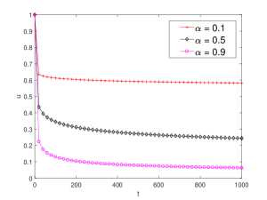
(a) Numerical solutions.

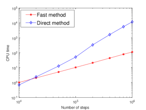
(b) Computational time.

Fig. 5: Numerical solutions and the computational time of the two different convolutions for Case II, $\tau=0.01,B=5,m=2,\sigma_{k}=k\alpha$.

Next, we consider a system of FODEs each having a different fractional index.

Example 5.2.

Consider the following system of fractional differential equations each with different fractional index

(54) $$\left\{\begin{aligned} &{}_{C}D^{\alpha_{1}}_{0,t}u(t)=w+(v-c_{1})u,\\ &{}_{C}D^{\alpha_{2}}_{0,t}v(t)=1-c_{2}v-u^{2},\\ &{}_{C}D^{\alpha_{3}}_{0,t}w(t)=-u-c_{3}w,\end{aligned}\right.$$

where $0<\alpha_{k}\leq 1\,(k=1,2,3)$, $c_{1},c_{2}$ and $c_{3}$ are positive constants, $c_{2}>1/2$.

Let $U_{n},V_{n}$ and $W_{n}$ be the approximate solutions of $u(t_{n}),v(t_{n})$ and $w(t_{n})$, respectively. Then the fully discrete scheme for the system (54) is given by:

(55) $$\left\{\begin{aligned} &{}_{F}D^{(-\alpha_{1},n,m)}_{\Delta T,\tau}U-{u_{0}t_{n}^{-\alpha_{1}}}/{\Gamma(1-\alpha_{1})}=W_{n}+(V_{n}-c_{1})U_{n},\\ &{}_{F}D^{(-\alpha_{2},n,m)}_{\Delta T,\tau}V-{v_{0}t_{n}^{-\alpha_{2}}}/{\Gamma(1-\alpha_{2})}=1-c_{2}V_{n}-U_{n}^{2},\\ &{}_{F}D^{(-\alpha_{3},n,m)}_{\Delta T,\tau}W-{w_{0}t_{n}^{-\alpha_{3}}}/{\Gamma(1-\alpha_{3})}=-U_{n}-c_{3}W_{n},\end{aligned}\right.$$

where $n\geq 2$ and ${}_{F}D^{(\alpha,n,m)}_{\Delta T,\tau}U$ is defined by (37). Because we use quadratic interpolation, $U_{k},V_{k},W_{k}$ for $k=1,2$ need to be known, which can be derived using the known methods with smaller stepsize. Here we use the L1 method with one correction term and smaller stepsize $\tau^{2}$ to derive these values. We take ${\Delta T}=\tau$ and $B=5$ in numerical simulations of this example.

If $\alpha_{1}=\alpha_{2}=\alpha_{3}=\alpha$, then (54) is just the fractional Lorenz system [36]. It has been proved that the fractional Lorenz system (54) is dissipative [36] and has an absorbing set defined by a ball $B(0,\sqrt{a/b}+\hat{\epsilon})$, where $a=1/2$ and $b=\min\{c_{1},c_{2}-1/2,c_{3}\}$. We take $c_{1}=1/4,c_{2}=1,c_{3}=1/4$ and the initial conditions as those in [36], i.e., $U_{0}=u(0)=2,V_{0}=v(0)=0.9,W_{0}=w(0)=0.2$, the time stepsize is taken as $\tau=0.01$. We compute numerical solutions for $t\in[0,1000]$, which is much larger than that in [36]. Numerical solutions for $\alpha=0.9$ are shown in Figure 6. We can easily find that $U_{n}^{2}+V_{n}^{2}+W_{n}^{2}<2$, which means $(U_{n},V_{n},W_{n})\in B(0,\sqrt{2})$. For other fractional orders $\alpha_{k}=\alpha$, we have similar results, see also [36]. Next, we choose different $\alpha_{1},\alpha_{2}$, and $\alpha_{3}$, and exhibit the numerical solutions in Figure 7 for $(\alpha_{1},\alpha_{2},\alpha_{3})=(0.9,0.8,0.7)$ and $(\alpha_{1},\alpha_{2},\alpha_{3})=(0.7,0.8,0.9)$. We can see that the numerical solutions $(U_{n},V_{n},W_{n})$ are also in a ball. For other choices of the fractional orders, we have similar results, which are not provided here.

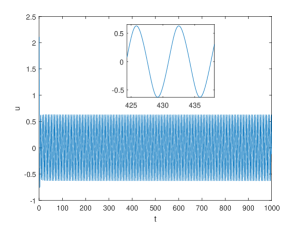
(a)

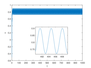
(b)

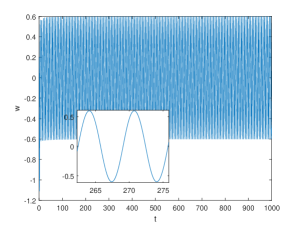
(c)

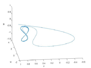
(d)

Fig. 6: Numerical solutions for Example 5.2, $\tau=0.01,m=2,\sigma_{k}=k\alpha,\alpha=0.9$.

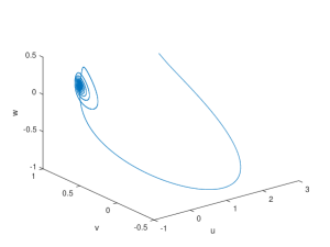
(a) $(\alpha_{1},\alpha_{2},\alpha_{3})=(0.9,0.8,0.7)$.

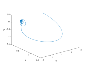
(b) $(\alpha_{1},\alpha_{2},\alpha_{3})=(0.7,0.8,0.9)$.

Fig. 7: Numerical solutions for Example 5.2, $t\in[0,1000]$, $\tau=0.01,m=0$.

6 Conclusion and discussion

We propose a unified fast memory-saving time-stepping method for both fractional integral and derivative operators, which is applied to solve FDEs. We generalize the fast convolution in [22] for fractional operators, while we use the (truncated) LG quadrature to discretize the kernel in the fractional operators instead of the trapezoidal rule in [22]. We also introduced correction terms in the fast method such that the non-smooth solutions of the considered FDEs can be resolved accurately. The present fast method has $O(n_{0}+\sum_{\ell}^{L}{q}_{\alpha}(N_{\ell}))$ active memory and $O(n_{0}n_{T}+(n_{T}-n_{0})\sum_{\ell}^{L}{q}_{\alpha}(N_{\ell}))$ operations. If a suitable memory length $\Delta T$ and a very large basis $B$ are applied, then the present fast method is similar to that in [14, 18], that is, the kernel $k_{\alpha}(t)$ is approximated via the truncated LG quadrature for all $t\in[\Delta T,T]$.

We present the error analysis of the present fast method. For a given precision, a criteria on how to choose the parameters used in the fast method is given explicitly, which works very well in numerical simulations.

We considered the fast method for the fractional operator of order $\alpha<1$. In fact, our method can be extended to the fractional integral of order greater than one. For example, for $\alpha\in[1,2)$, Eq. (4) still holds in the sense of the finite part integral, that is, Eq. (4) is equivalent to $k_{\alpha}(t)=\frac{t}{\Gamma(\alpha)\Gamma(2-\alpha)}\int_{0}^{\infty}\lambda^{1-\alpha}e^{-t\lambda}\,{\rm d}\lambda.$ In such a case, a coupled ODEs are needed to be resolved instead of one for $\alpha<1$.

In the future, we will apply the fast method to solve a large system of time-fractional PDEs, perhaps in three spatial dimensions. We will also explore how to efficiently calculate the discrete convolution $\sum_{k=0}^{n}\omega_{n-k}u(t_{k})$, where the quadrature weights $\{\omega_{n}\}$ are not from the interpolation as done in the present work, but from the generating functions, see, [21].

Appendix A Proofs

Proof of Theorem 1.

Proof.

We follow the proof of Theorem 2.2 in [39]. We first expand $g(\lambda)=e^{-t\lambda}$ in terms of the Laguerre polynomials, i.e., $g(\lambda)=\sum_{n=0}^{\infty}a_{n}L_{n}^{(\alpha)}(\lambda),$ where

$$a_{n}=\frac{\Gamma(n+1)}{\Gamma(n+1+\alpha)}\int_{0}^{\infty}\lambda^{\alpha}e^{-\lambda}g(\lambda)\,{\rm d}\lambda=\frac{t^{n}}{(t+1)^{n+1+\alpha}}.$$

The following property will be used, see [39],

$$\big{|}Q_{N}^{\alpha}[L_{n}^{(\alpha)}]\big{|}\leq\left\{\begin{aligned} &2\Gamma(1+\alpha),{\quad}-1<\alpha\leq 0,\\ &2^{1+\alpha}{\Gamma(n+1+\alpha)}/{\Gamma(n+1)},{\quad}\alpha>0.\end{aligned}\right.$$

With the above two equations and $I^{\alpha}[e^{-t\lambda}]-Q_{N}^{\alpha}[e^{-t\lambda}]=\sum_{n=2N}^{\infty}a_{n}Q_{N}^{\alpha}[L_{n}^{(\alpha)}]$ gives

(56) $$\big{|}I^{\alpha}[e^{-t\lambda}]-Q_{N}^{\alpha}[e^{-t\lambda}]\big{|}\leq\left\{\begin{aligned} &2^{1+\alpha}\Gamma(1+\alpha)\sum_{n=2N}^{\infty}a_{n},{\quad}-1<\alpha\leq 0,\\ &c_{\alpha}2^{1+\alpha}\sum_{n=2N}^{\infty}n^{\alpha}a_{n},{\quad}\alpha>0.\end{aligned}\right.$$

Let $q=t/(1+t)$. Then we have $\sum_{n=2N}^{\infty}a_{n}=(1+t)^{-\alpha}q^{2N}$ for $-1<\alpha\leq 0$. For $\alpha>0$, one hase

$$\sum_{n=2N}^{\infty}n^{\alpha}a_{n}=(1+t)^{-\alpha}q^{2N}(2N)^{\alpha}\sum_{n=0}^{\infty}q^{n}\Big{(}1+\frac{n}{2N}\Big{)}^{\alpha}\leq C_{\alpha,t}2^{\alpha}(1+t)^{1-\alpha}q^{2N}N^{\alpha},$$

where $C_{\alpha,t}=\sum_{n=0}^{\infty}(n+2)^{\alpha}q^{2Nn}$ is used. With the above equation and (56) yields (41) for $T=1$. Using the following relation

$$\big{|}I^{\alpha}[T,e^{-t\lambda}]-Q_{N}^{\alpha}[T,e^{-t\lambda}]\big{|}=T^{-\alpha-1}\big{|}I^{\alpha}[e^{-(t/T)\lambda}]-Q_{N}^{\alpha}[e^{-(t/T)\lambda}]\big{|}$$

leads to (41) for any $T>0$. The proof is complete. ∎

Proof of Theorem 2.

Proof.

The following results can be found in [12],

(57) $${\lambda}_{j}<\frac{2j+\alpha+3}{2N+\alpha+3}\Big{(}2j+\alpha+3+\sqrt{(2j+\alpha+3)^{2}+0.25-\alpha^{2}}\Big{)},$$

(58) $${\lambda}_{j}>\frac{2(J_{\alpha,j}/2)^{2}}{2N+\alpha+3},{\quad}J_{\alpha,j}=\pi(j+3/4+\alpha/2)+O(j^{-1}),$$

where (58) holds when $j$ is sufficiently large. For a sufficiently large $N$, the Laguerre polynomial satisfies (see (7.14) in [32])

(59) $$\big{|}L^{(\alpha)}_{N}(x)\big{|}\approx\pi^{-1/2}(Nx)^{-1/4}e^{x/2},{\quad}\forall x\geq 0.$$

With (57)–(59) and (40), we have the following estimate

(60) $${w}^{(\alpha)}_{j}\leq C_{\alpha}(N+1)^{\alpha}\left(\frac{j+1}{N+1}\right)^{3}e^{-{\lambda}_{j}}\leq C(N+1)^{\alpha}e^{-{\lambda}_{j}},$$

for sufficiently large $j$, where ${\lambda}_{j}=\theta_{j}(j+1)^{2}/(N+1)$ and $\theta_{j}$ is bounded and approximately between $\pi^{2}/4$ and $4$. The proof is completed. ∎

References

- [1] D. Baffet and J. S. Hesthaven, High-order accurate adaptive kernel compression time-stepping schemes for fractional differential equations, J. Sci. Comput., 72 (2017), pp. 1169–1195.
- [2] D. Baffet and J. S. Hesthaven, A kernel compression scheme for fractional differential equations, SIAM J. Numer. Anal., 55 (2017), pp. 496–520.
- [3] L. Banjai, M. López-Fernández, and A. Schädle, Fast and oblivious algorithms for dissipative and two-dimensional wave equations, SIAM J. Numer. Anal., 55 (2017), pp. 621–639.
- [4] G. Beylkin and L. Monz n, Approximation by exponential sums revisited, Appl. Comput. Harmon. Anal., 28 (2010), pp. 131–149.
- [5] L. D’Amore, A. Murli, and M. Rizzardi, An extension of the Henrici formula for Laplace transform inversion, Inverse Problems, 16 (2000), pp. 1441–1456.
- [6] W. Deng, Short memory principle and a predictor-corrector approach for fractional differential equations, J. Comput. Appl. Math., 206 (2007), pp. 174–188.
- [7] K. Diethelm, Generalized compound quadrature formulae for finite-part integrals, IMA J. Numer. Anal., 17 (1997), pp. 479–493.
- [8] , The analysis of fractional differential equations, Springer-Verlag, Berlin, 2010.
- [9] K. Diethelm, J. M. Ford, N. J. Ford, and M. Weilbeer, Pitfalls in fast numerical solvers for fractional differential equations, J. Comput. Appl. Math., 186 (2006), pp. 482–503.
- [10] N. J. Ford and A. C. Simpson, The numerical solution of fractional differential equations: Speed versus accuracy, Numerical Algorithms, 26 (2001), pp. 333–346.
- [11] L. Galeone and R. Garrappa, Fractional Adams-Moulton methods, Math. Comput. Simulation, 79 (2008), pp. 1358–1367.
- [12] L. Gatteschi, Asymptotics and bounds for the zeros of laguerre polynomials: a survey, J. Comput. Appl. Math., 144 (2002), pp. 7–27.
- [13] H. Jiang, F. Liu, I. Turner, and K. Burrage, Analytical solutions for the multi-term time-fractional diffusion-wave/diffusion equations in a finite domain, Comput. Math. Appl., 64 (2012), pp. 3377–3388.
- [14] S. Jiang, J. Zhang, Q. Zhang, and Z. Zhang, Fast evaluation of the Caputo fractional derivative and its applications to fractional diffusion equations, Commun. Comput. Phys., 21 (2017), pp. 650–678.
- [15] B. Jin, R. Lazarov, and Z. Zhou, An analysis of the L1 scheme for the subdiffusion equation with nonsmooth data, IMA J. Numer. Anal., 36 (2016), pp. 197–221.
- [16] C. Li, Q. Yi, and A. Chen, Finite difference methods with non-uniform meshes for nonlinear fractional differential equations, J. Comput. Phys., 316 (2016), pp. 614–631.
- [17] C. Li and F. Zeng, Numerical methods for fractional calculus, CRC Press, Boca Raton, FL, 2015.
- [18] J.-R. Li, A fast time stepping method for evaluating fractional integrals, SIAM J. Sci. Comput., 31 (2010), pp. 4696–4714.
- [19] Z. Li, Z. Liang, and Y. Yan, High-order numerical methods for solving time fractional partial differential equations, J. Sci. Comput., 71 (2017), pp. 785–803.
- [20] M. López-Fernández, C. Lubich, and A. Schädle, Adaptive, fast, and oblivious convolution in evolution equations with memory, SIAM J. Sci. Comput., 30 (2008), pp. 1015–1037.
- [21] C. Lubich, Discretized fractional calculus, SIAM J. Math. Anal., 17 (1986), pp. 704–719.
- [22] C. Lubich and A. Schädle, Fast convolution for nonreflecting boundary conditions, SIAM J. Sci. Comput., 24 (2002), pp. 161–182.
- [23] Y. Luchko, Initial-boundary problems for the generalized multi-term time-fractional diffusion equation, J. Math. Anal. Appl., 374 (2011), pp. 538–548.
- [24] C. Lv and C. Xu, Error analysis of a high order method for time-fractional diffusion equations, SIAM J. Sci. Comput., 38 (2016), pp. A2699–A2724.
- [25] W. McLean, Fast summation by interval clustering for an evolution equation with memory, SIAM J. Sci. Comput., 34 (2012), pp. A3039–A3056.
- [26] , Exponential sum approximations for , (2016), p. arXiv:1606.00123.
- [27] W. McLean and K. Mustapha, A second-order accurate numerical method for a fractional wave equation, Numer. Math., 105 (2007), pp. 481–510.
- [28] R. Metzler and J. Klafter, The random walk’s guide to anomalous diffusion: a fractional dynamics approach, Phys. Rep., 339 (2000), p. 77.
- [29] I. Podlubny, Fractional differential equations, Academic Press, Inc., San Diego, CA, 1999.
- [30] S. G. Samko, A. A. Kilbas, and O. I. Marichev, Fractional integrals and derivatives: Theory and applications, Gordon and Breach Science Publishers, Yverdon, 1993.
- [31] A. Schädle, M. López-Fernández, and C. Lubich, Fast and oblivious convolution quadrature, SIAM J. Sci. Comput., 28 (2006), pp. 421–438.
- [32] J. Shen, T. Tang, and L.-L. Wang, Spectral methods, vol. 41 of Springer Series in Computational Mathematics, Springer, Heidelberg, 2011. Algorithms, analysis and applications.
- [33] M. Stynes, E. O’Riordan, and J. L. Gracia, Error analysis of a finite difference method on graded meshes for a time-fractional diffusion equation, SIAM J. Numer. Anal., 55 (2017), pp. 1057–1079.
- [34] Z.-z. Sun and X. Wu, A fully discrete difference scheme for a diffusion-wave system, Appl. Numer. Math., 56 (2006), pp. 193–209.
- [35] C.-L. Wang, Z.-Q. Wang, and H.-L. Jia, An hp-version spectral collocation method for nonlinear Volterra integro-differential equation with weakly singular kernels, J. Sci. Comput., (2017), pp. 1–32.
- [36] D. Wang and A. Xiao, Dissipativity and contractivity for fractional-order systems, Nonlinear Dynamics, 80 (2015), pp. 287–294.
- [37] J. A. C. Weideman, Optimizing talbot s contours for the inversion of the laplace transform, SIAM J. Numer. Anal., 44 (2006), pp. 2342–2362.
- [38] J. A. C. Weideman and L. N. Trefethen, Parabolic and hyperbolic contours for computing the bromwich integral, Math. Comp., 76 (2007), pp. 1341–1356.
- [39] S. Xiang, Asymptotics on Laguerre or Hermite polynomial expansions and their applications in Gauss quadrature, J. Math. Anal. Appl., 393 (2012), pp. 434–444.
- [40] Y. Yan, Z.-Z. Sun, and J. Zhang, Fast evaluation of the caputo fractional derivative and its applications to fractional diffusion equations: A second-order scheme, Commun. Comput. Phys., 22 (2017), pp. 1028–1048.
- [41] Y. Yu, P. Perdikaris, and G. E. Karniadakis, Fractional modeling of viscoelasticity in 3d cerebral arteries and aneurysms, J. Comput. Phys., 323 (2016), pp. 219–242.
- [42] M. Zayernouri and A. Matzavinos, Fractional Adams-Bashforth/Moulton methods: An application to the fractional Keller-Segel chemotaxis system, J. Comput. Phys., 317 (2016), pp. 1–14.
- [43] F. Zeng, Z. Zhang, and G. E. Karniadakis, Fast difference schemes for solving high-dimensional time-fractional subdiffusion equations, J. Comput. Phys., 307 (2016), pp. 15–33.
- [44] F. Zeng, Z. Zhang, and G. E. Karniadakis, Second-order numerical methods for multi-term fractional differential equations: Smooth and non-smooth solutions, Comput. Methods Appl. Mech. Engrg., (2017), p. in press.