Multiobjective optimization to a TB-HIV/AIDS coinfection optimal control problem

Abstract

We consider a recent coinfection model for Tuberculosis (TB), Human Immunodeficiency Virus (HIV) infection and Acquired Immunodeficiency Syndrome (AIDS) proposed in [Discrete Contin. Dyn. Syst. 35 (2015), no. 9, 4639–4663]. We introduce and analyze a multiobjective formulation of an optimal control problem, where the two conflicting objectives are: minimization of the number of HIV infected individuals with AIDS clinical symptoms and coinfected with AIDS and active TB; and costs related to prevention and treatment of HIV and/or TB measures. The proposed approach eliminates some limitations of previous works. The results of the numerical study provide comprehensive insights about the optimal treatment policies and the population dynamics resulting from their implementation. Some nonintuitive conclusions are drawn. Overall, the simulation results demonstrate the usefulness and validity of the proposed approach.

Keywords: Tuberculosis; HIV; Epidemic model; Treatment strategies; Optimal control theory; Multiobjective optimization.

2010 Mathematics Subject Classification: 90C29; 92C50.

1 Introduction

The human immunodeficiency virus (HIV) is a retrovirus that infects cells of the immune system, destroying or impairing their function. HIV is transmitted primarily via unprotected sexual intercourse, contaminated blood transfusions, hypodermic needles, and from mother to child during pregnancy, delivery, or breastfeeding [23]. As the infection progresses, the immune system becomes weaker, and the person becomes more susceptible to infections. The most advanced stage of HIV infection is acquired immunodeficiency syndrome (AIDS) [29]. There is no cure or vaccine to AIDS. However, antiretroviral (ART) treatment improves health, prolongs life, and substantially reduces the risk of HIV transmission. In both high-income and low-income countries, the life expectancy of patients infected with HIV who have access to ART is now measured in decades, and might approach that of uninfected populations in patients who receive an optimum treatment (see [4] and references cited therein). However, ART treatment still presents substantial limitations: does not fully restore health; treatment is associated with side effects; the medications are expensive; and is not curative. Following the Joint United Nations Programme on HIV and AIDS (UNAIDS), in 2013 there were approximately 35 million people living with HIV globally. An estimated 2.1 million people became newly infected with HIV in 2013, down from 3.4 million in 2001 worldwide. The number of new HIV infection among children has declined 58% since 2001, being in 2013 approximately 240 000 worldwide. The number of AIDS-related deaths have fallen by 35% since the peak in 2005. In 2013, approximately 1.5 million people died from AIDS-related causes worldwide. In 2013, around 12.9 million people living with HIV had access to ART therapy, which represents, approximately, 37% of all people living with HIV [26, 28].

Mycobacterium tuberculosis is the cause of most occurrences of tuberculosis (TB) and is usually acquired via airborne infection from someone who has active TB. It typically affects the lungs (pulmonary TB) but can affect other sites as well (extrapulmonary TB). According with the World Health Organization (WHO), in 2013, an estimated 9.0 million people developed TB and 1.5 million died from the disease, 360 000 of whom were HIV-positive. TB is slowly declining each year and it is estimated that 37 million lives were saved between 2000 and 2013 through effective diagnosis and treatment. However, since most deaths from TB are preventable, the death toll from the disease is still unacceptably high and efforts to combat it must be accelerated [31].

Following WHO, the human immunodeficiency virus (HIV) and mycobacterium tuberculosis are the first and second cause of death from a single infectious agent, respectively [30]. Both HIV/AIDS and TB are present in all regions of the world [17, 31]. Individuals infected with HIV are more likely to develop TB disease because of their immunodeficiency, and HIV infection is the most powerful risk factor for progression from TB infection to disease [9]. In 2013, 1.1 million of 9.0 million people who developed TB worldwide were HIV-positive. The number of people dying from HIV-associated to TB has been falling since 2003. However, there were still 360 000 deaths from HIV-associated to TB in 2013, and further efforts are needed to reduce this burden [31]. ART is a critical intervention for reducing the risk of TB morbidity and mortality among people living with HIV and, when combined with TB preventive therapy, it can have a significant impact on TB prevention [31]. Collaborative TB/HIV activities (including HIV testing, ART therapy and TB preventive measures) are crucial for the reduction of TB-HIV coinfected individuals. WHO estimates that these collaborative activities prevented 1.3 million people from dying, from 2005 to 2012. However, significant challenges remain: the reduction of tuberculosis related deaths among people living with HIV has slowed in recent years; the ART therapy is not being delivered to TB-HIV coinfected patients in the majority of the countries with the largest number of TB/HIV patients; the pace of treatment scale-up for TB/HIV patients has slowed; less than half of notified TB patients were tested for HIV in 2012; and only a small fraction of TB/HIV infected individuals received TB preventive therapy [27]. The study of the joint dynamics of TB and HIV present formidable mathematical challenges due to the fact that the models of transmission are quite distinct [22]. Here we focus on a recent mathematical model of optimal control for TB-HIV/AIDS coinfection proposed by [25].

Optimal control is a branch of mathematics developed to find optimal ways to control a dynamic system [20], e.g. a dynamic system that models infectious diseases. Optimal control has been applied to TB models, HIV models and also co-infection models (see, e.g., [1, 11, 12, 13, 14, 21, 24, 25] and references cited therein for TB-HIV/AIDS models and [18] for co-infection of malaria and cholera). In this paper we consider the optimal control problem for the TB-HIV/AIDS model proposed in [25] from a multiobjective perspective. Our approach avoids the use of weight parameters and allows to obtain a wide range of optimal control strategies. These strategies offer the decision maker useful information for effective decision making.

Traditional mathematical programming methods for solving multiobjective optimization problems (MOPs) convert the original problem into a single-objective optimization problem. This is referred as to scalarization and the function to be optimized, which depends on some parameters, is termed the scalarizing function. A solution to the scalarizing function, obtained using a single-objective optimization algorithm, is expected to be Pareto optimal. For approximating multiple Pareto optimal solutions, repeated runs with different parameter settings must be performed. The weighted sum method [8] consists in minimizing a weighted sum of multiple objectives. For problems with a convex Pareto front, this method guarantees finding solutions in the entire Pareto optimal region. However, it fails to find solutions in nonconvex regions of the Pareto front. Weighted metric methods [16] are based on minimizing a weighted distance between some reference point and the feasible objective region. The widely used approach belonging to this class of methods is the Chebyshev method [2], which consists in minimizing a weighted infinity norm. Although solutions in convex and nonconvex regions of the Pareto front can be obtained by this method, a resulting scalarizing function becomes nondifferentiable even when all the objectives are differentiable. The problem resulting from the Chebyshev method can be reformulated in the smooth form. The resulting formulation is known as the goal attainment method [16] or the Pascoletti–Serafini scalarization [19]. In this method, a slack variable is minimized and the weighted difference for each objective is converted into a constraint. Although the problem can be solved in a differentiable form, problem complexity is augmented by adding one additional variable and $m$ constraints (where $m$ is the number of objectives). The normal boundary intersection and normal constraint methods use a hyperplane with uniformly distributed points passing through the critical points of the Pareto front. The normal boundary intersection method [3] searches for the maximum distance from a point on the simplex along the normal pointing toward the origin. The obtained point may or may not be a Pareto optimal point, with the resulting scalarizing problem including an equality constraint that is not easy to treat for all the cases. On the other hand, the normal constraint method [15] uses an inequality constraint reduction of the feasible objective space and the normalized function values to cope with disparate function scales. The method is successful in achieving a uniform distribution of approximating points, though there is no guarantee that an obtained point is Pareto optimal. Here, motivated by the results recently obtained in [7] for a TB model and in [5, 6] for the dengue disease, we adopt the $\epsilon$-constraint method [10]. This method suggests optimizing one objective function and converting all other objectives as constraints, setting an upper bound to each of them. Solutions obtained using multiobjective optimization provide comprehensive insights about the optimal strategies and the diseases dynamics resulting from implementation of those strategies.

The paper is organized as follows. In Section 2 we briefly describe the TB-HIV/AIDS model from [25]. The multiobjective optimization theory is applied to an optimal control problem in Section 3: we start by formulating the optimal control problem in Subsection 3.1, then we consider this problem from a multiobjective perspective (Subsection 3.2) and we describe the numerical method that we use to solve the multiobjective problem (Subsection 3.3). In Section 4 we present and discuss numerical results for the multiobjective problem. We end with Section 5 of conclusions and future work.

2 TB-HIV/AIDS coinfection model

The present study considers the population model for TB-HIV/AIDS coinfection proposed in [25], where TB, HIV and TB-HIV infected individuals have access to respective disease treatment, and single HIV-infected and TB-HIV co-infected individuals under HIV and TB/HIV treatment, respectively, stay in a chronic stage of the HIV infection. The model divides the population into eleven mutually exclusive compartments: susceptible individuals ($S$); TB-latently infected individuals, who have no symptoms of TB disease and are not infectious ($L_{T}$); TB-infected individuals, who have active TB disease and are infectious ($I_{T}$); TB-recovered individuals ($R$); HIV-infected individuals with no clinical symptoms of AIDS ($I_{H}$); HIV-infected individuals under treatment for HIV infection ($C_{H}$); HIV-infected individuals with AIDS clinical symptoms ($A$); TB-latent individuals co-infected with HIV (pre-AIDS) ($L_{TH}$); HIV-infected individuals (pre-AIDS) co-infected with active TB disease ($I_{TH}$); TB-recovered individuals with HIV-infection without AIDS symptoms ($R_{H}$); and HIV-infected individuals with AIDS symptoms co-infected with active TB ($A_{T}$). The total population at time $t$, denoted by $N(t)$, is given by

$$N(t)=S(t)+L_{T}(t)+I_{T}(t)+R(t)+I_{H}(t)+A(t)+C_{H}(t)\\ +L_{TH}(t)+I_{TH}(t)+R_{H}(t)+A_{T}(t).$$

Susceptible individuals acquire TB infection from individuals with active TB at a rate $\lambda_{T}$, given by

$$\lambda_{T}(t)=\frac{\beta_{1}}{N(t)}(I_{T}(t)+I_{TH}(t)+A_{T}(t)),$$

where $\beta_{1}$ is the effective contact rate for TB infection. Similarly, susceptible individuals acquire HIV infection, following effective contact with people infected with HIV at a rate $\lambda_{H}$, given by

$$\lambda_{H}(t)=\frac{\beta_{2}}{N(t)}[I_{H}(t)+I_{TH}(t)+L_{TH}(t)+R_{H}(t)+\eta_{C}C_{H}(t)+\eta_{A}(A(t)+A_{T}(t))],$$

where $\beta_{2}$ is the effective contact rate for HIV transmission, $\eta_{A}\geq 1$ is the modification parameter that accounts for the relative infectiousness of individuals with AIDS symptoms and $\eta_{C}\leq 1$ is the modification parameter that translates the partial restoration of immune function of individuals with HIV infection that use correctly the antiretroviral treatment. The remaining parameters used to describe the model are presented in Table 1.

Symbol	Description	Value
$T$	Considered time in years	10
$N(0)$	Initial population size	30000
$\gamma_{1}$	Modification parameter	0.9
$\gamma_{2}$	Modification parameter	1.1
$\eta_{C}$	Modification parameter	0.9
$\eta_{A}$	Modification parameter	1.05
$\delta$	Modification parameter	1.03
$\psi$	Modification parameter	1.07
$\beta_{1}$	TB transmission rate	0.6
$\beta_{2}$	HIV transmission rate	0.1
$\mu$	Recruitment rate	430.0
$k_{1}$	Rate at which individuals leave $L_{T}$ class by becoming infectious	1.0/2.0
$k_{2}$	Rate at which individuals leave $L_{TH}$ class by becoming TB infectious	$1.3k_{1}$
$k_{3}$	Rate at which individuals leave $L_{TH}$ class	2.0
$\rho_{1}$	Rate at which individuals leave $I_{H}$ class to $A$	0.1
$\rho_{2}$	Rate at which individuals leave $I_{TH}$ class	1.0
$\omega_{1}$	Rate at which individuals leave $C_{H}$ class	0.09
$\omega_{2}$	Rate at which individuals leave $R_{H}$ class	0.15
$\tau_{1}$	TB treatment rate for $L_{T}$ individuals	2.0
$\tau_{2}$	TB treatment rate for $I_{T}$ individuals	1.0
$\phi$	HIV treatment rate for $I_{H}$ individuals	1.0
$\alpha_{1}$	AIDS treatment rate	0.33
$\alpha_{2}$	HIV treatment rate for $A_{T}$ individuals	0.33
$r$	Fraction of $L_{TH}$ individuals that take HIV and TB treatment	0.3
$d_{N}$	Natural death rate	1.0/70.0
$d_{T}$	TB induced death rate	1.0/10.0
$d_{A}$	AIDS induced death rate	0.3
$d_{TA}$	AIDS-TB induced death rate	0.33

Table 1: Model parameters, borrowed from [25].

Two control functions, which represent prevention and treatment measures, are introduced into the model and are continuously implemented during a considered period of disease treatment: the control $u_{1}(t)$ represents the fraction of $I_{TH}$ individuals that takes HIV and TB treatment, simultaneously; $u_{2}(t)$ represents the fraction of $I_{TH}$ individuals that takes TB treatment only [25].

The transmission dynamics of TB-HIV/AIDS coinfection is modeled by the following system of differential equations:

$$\small\left\{\begin{array}[]{l}\dot{S}(t)=\mu-\lambda_{T}(t)S(t)-\lambda_{H}(t)S(t)-d_{N}S(t),\\ \dot{L}_{T}(t)=\lambda_{T}(t)S(t)+\gamma_{1}\lambda_{T}(t)R(t)-(k_{1}+\tau_{1}+d_{N})L_{T}(t),\\ \dot{I}_{T}(t)=k_{1}L_{T}(t)-(\tau_{2}+d_{T}+d_{N}+\delta\lambda_{H}(t))I_{T}(t),\\ \dot{R}(t)=\tau_{1}L_{T}(t)+\tau_{2}I_{T}(t)-(\gamma_{1}\lambda_{T}(t)+\lambda_{H}(t)+d_{N})R(t),\\ \dot{I}_{H}(t)=\lambda_{H}(t)S(t)-(\rho_{1}+\phi+\psi\lambda_{T}(t)+d_{N})I_{H}(t)+\alpha_{1}A(t)+\lambda_{H}(t)R(t)+\omega_{1}C_{H}(t),\\ \dot{A}(t)=\rho_{1}I_{H}(t)+\omega_{2}R_{H}(t)-\alpha_{1}A(t)-(d_{N}+d_{A})A(t),\\ \dot{C}_{H}(t)=\phi I_{H}(t)+u_{1}(t)\rho_{2}I_{TH}(t)+rk_{3}L_{TH}(t)-(\omega_{1}+d_{N})C_{H}(t),\\ \dot{L}_{TH}(t)=\gamma_{2}\lambda_{T}(t)R_{H}(t)-(k_{2}+k_{3}+d_{N})L_{TH}(t),\\ \dot{I}_{TH}(t)=\delta\lambda_{H}(t)I_{T}(t)+\psi\lambda_{T}(t)I_{H}(t)+\alpha_{2}A_{T}(t)+k_{2}L_{TH}(t)-(\rho_{2}+d_{N}+d_{T})I_{TH}(t),\\ \dot{R}_{H}(t)=u_{2}(t)\rho_{2}I_{TH}(t)+(1-r)k_{3}L_{TH}(t)-(\gamma_{2}\lambda_{T}(t)+\omega_{2}+d_{N})R_{H}(t),\\ \dot{A}_{T}(t)=(1-(u_{1}(t)+u_{2}(t)))\rho_{2}I_{TH}(t)-(\alpha_{2}+d_{N}+d_{TA})A_{T}(t).\end{array}\right.$$ (1)

The model flow is illustrated in Figure 1.

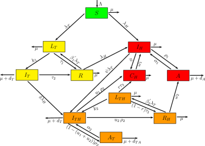
Figure 1: Model for TB-HIV/AIDS transmission.

The initial conditions are given in Table 2.

Cathegory	Description	Initial Value
$S$	Susceptible	$\frac{66N(0)}{120}$
${L}_{T}$	TB-Latent	$\frac{37N(0)}{120}$
$I_{T}$	TB-Active infected	$\frac{5N(0)}{120}$
$R$	TB-Recovered	$\frac{37N(0)}{120}$
$I_{H}$	HIV-Infected (pre-AIDS)	$\frac{2N(0)}{120}$
$A$	HIV-infected with AIDS symptoms	$\frac{37N(0)}{120}$
$C_{H}$	HIV-infected under ART therapy	$\frac{N(0)}{120}$
$L_{TH}$	TB-Latent co-infected with HIV (pre-AIDS)	$\frac{2N(0)}{120}$
$I_{TH}$	HIV-Infected (pre-AIDS) co-infected with active TB	$\frac{2N(0)}{120}$
$R_{H}$	TB-recovered with HIV-infection (pre-AIDS)	$\frac{N(0)}{120}$
$A_{T}$	HIV-Infected with AIDS symptoms co-infected with active TB	$\frac{N(0)}{120}$

Table 2: Initial conditions for the state variables of the TB-HIV/AIDS model (1), borrowed from [25].

Note that the period spent in class $I_{TH}$ does not change with the control measures because the controls represent the fraction of individuals that are treated both for TB and HIV and only for TB, and not the treatment duration. Indeed, the period spent in class $I_{TH}$ is given by the constant treatment rate $\rho_{2}$.

3 Multiobjective approach to an optimal control problem

Traditionally, the problem of finding a control law for a given system is addressed by optimal control theory [20].

3.1 Optimal control problem

In the optimal control approach, the aim is to find the optimal values $u_{1}^{*}$ and $u_{2}^{*}$ of the controls $u_{1}$ and $u_{2}$, such that the associated state trajectories $S^{*}$, $L_{T}^{*}$, $I_{T}^{*}$, $R^{*}$, $I_{H}^{*}$, $A^{*}$, $C_{H}^{*}$, $L_{TH}^{*}$, $I_{TH}^{*}$, $R_{H}^{*}$, $A_{T}^{*}$, are solution of system (1) in the time interval $[0,T]$, with the initial conditions in Table 2, and minimize an objective functional. Consider the state system of ordinary differential equations (1) and the set of admissible control functions given by

$$\Omega=\{(u_{1}(\cdot),u_{2}(\cdot))\in(L^{\infty}(0,T))^{2}\,|\, 0\leq u_{1}(t),u_{2}(t)\leq 0.95$$

$$\,\wedge\,u_{1}(t)+u_{2}(t)\leq 0.95,\,\forall t\in[0,T]\}.$$

According to [25], the objective functional can be defined as

$$J(u_{1}(\cdot),u_{2}(\cdot))=\int_{0}^{T}\left[A(t)+A_{T}(t)+w_{1}u_{1}^{2}(t)+w_{2}u_{2}^{2}(t)\right]dt,$$ (2)

where the constants $w_{1}$ and $w_{2}$ are a measure of the relative cost of the interventions associated with the controls $u_{1}$ and $u_{2}$, respectively. Note that the objective functional (2) is a function of state and control variables. Its minimization implies three important aspects: (i) reducing the number of individuals with AIDS symptoms, (ii) decreasing the number of individuals with AIDS symptoms and active TB disease and (iii) reducing the costs of implementing treatment policies. The optimal control problem consists in determining ($S^{*}$, $L_{T}^{*}$, $I_{T}^{*}$, $R^{*}$, $I_{H}^{*}$, $A^{*}$, $C_{H}^{*}$, $L_{TH}^{*}$, $I_{TH}^{*}$, $R_{H}^{*}$, $A_{T}^{*}$), associated to admissible controls $\left(u_{1}^{*}(\cdot),u_{2}^{*}(\cdot)\right)\in\Omega$ on the time interval $[0,T]$, satisfying (1), the initial conditions in Table 2, and minimizing the objective functional (2), i.e.,

$$J(u_{1}^{*}(\cdot),u_{2}^{*}(\cdot))=\min_{\Omega}J(u_{1}(\cdot),u_{2}(\cdot)).$$

The approach based on optimal control theory adopted in [25] allows to obtain the optimal solution to the cost functional (2), which is defined from some decision maker’s perspective by means of the constants $w_{1}$ and $w_{2}$. However, the choice of the values of $w_{1}$ and $w_{2}$ requires some knowledge about the problem and the decision maker’s preferences, which often are not available in advance. Another disadvantage consists in the fact that a single optimal solution to (2) does not provide all useful insights about the optimal strategies and corresponding dynamics. A large range of alternatives remain unexplored and the decision maker is limited in his/her options. In [25], numerical simulations to the optimal control problem are performed using $(w_{1},w_{2})=(25,25)$ and $(w_{1},w_{2})=(250,25)$. Both values are larger than one, which suggests that they are adapted to the scale of the objectives. The choice of the values of these parameters is not straightforward and there is no guarantee that the best compromise solution has been obtained.

3.2 Multiobjective optimization

Our work addresses the optimal control problem for the TB-HIV/AIDS coinfection model (1) from a multiobjective perspective. A multiojective optimization problem is formulated by decomposing the cost functional shown in (2) into two components, representing different aspects that must be taken into consideration when dealing with TB-HIV/AIDS. The problem of finding the optimal controls is defined as:

$$\begin{array}[]{rl}\text{minimize}&f_{1}(A(\cdot),A_{T}(\cdot))=\displaystyle\int_{0}^{T}\left[A(t)+A_{T}(t)\right]dt,\\[5.69046pt] &f_{2}(u_{1}(\cdot),u_{2}(\cdot))=\displaystyle\int_{0}^{T}\left[u_{1}^{2}(t)+u_{2}^{2}(t)\right]dt,\\[5.69046pt] \text{subject to}&0\leq u_{1}(t)\leq 0.95,\\ &0\leq u_{2}(t)\leq 0.95,\\ &u_{1}(t)+u_{2}(t)\leq 0.95.\end{array}$$ (3)

In the above formulation, the weights are absent and the two objectives represent the medical and economical perspectives, respectively. This naturally reflects the conflicting nature of the underlying decision making problem, hence, solving (3) is interesting and challenging.

3.3 Scalarization

A traditional mathematical programming approach to solving a multiojective optimization problem consists in transforming an original problem with multiple objectives into a number of single-objective subproblems. This is referred to as scalarization. The transformation is performed by means of a scalarizing function with some user-defined parameters. A single Pareto optimal solution is sought by optimizing each subproblem. Repeated runs with different parameter settings for the scalarizing function are used to approximate multiple Pareto optimal solutions.

Several approaches to scalarization have been developed. They differ in the way the scalarizing function is formulated. The weighted sum method suggests minimizing a weighted sum of the objectives [8]. The limitation of this method is that solutions can only be obtained in convex regions of the Pareto front. On the other hand, the $\epsilon$-constraint method [10] suggests optimizing one objective function and converting all other objectives into constraints by setting an upper bound to each of them. This method can find solutions in both convex and nonconvex regions of the Pareto front. The method of weighted metrics [16] seeks to minimize the distance between the feasible objective region and some reference point. This method is also known as compromise programming [32]. For measuring the distance, a weighted $L_{p}$ norm is utilized. When the value of $p$ is small, the method may fail to find solutions in nonconvex regions. When $p=\infty$, the method defines the weighted Chebyshev problem [2]. This problem consists in minimizing the largest weighted deviation of one objective. By optimizing the weighted Chebyshev problem, solutions from convex and nonconvex regions can be generated. A major drawback is that even when the original MOP is differentiable, the resulting single-objective problem is nondifferentiable. Weakly Pareto optimal solutions can be also obtained [16]. A relaxed formulation of the Chebyshev problem with differentiable scalarizing function is known as the Pascoletti–Serafini scalarization [19]. Though, this method introduces one additional variable and one constraint for each objective function. The normal boundary intersection [3] uses a hyperplane with evenly distributed points that passes through the extreme points of the Pareto front. For each point on the hyperplane, the method searches for the maximum distance along the normal pointing toward the origin. The normal constraint method [15] suggests optimizing one objective and employing an inequality constraint reduction of the feasible space using the points on the hyperplane. However, there is no guarantee that the solutions obtained by the normal boundary intersection and normal constraint methods are Pareto optimal. A comparative analysis of the different scalarization approaches on optimal control problems from epidemiology can be found in [6, 7].

Motivated by the results recently obtained in [7] for a TB model, we adopt here the $\epsilon$-constraint method [10]. This method suggests optimizing one objective function while converting all other objectives into constraints by setting an upper bound to each of them. The problem to be solved is of the following form:

$$\begin{array}[]{rlll}\underset{\boldsymbol{x}\in\Omega}{\text{minimize}}&f_{l}(\boldsymbol{x})&\\ \text{subject to}&f_{i}(\boldsymbol{x})\leq\epsilon_{i},&\forall i\in\{1,\ldots,m\}\wedge i\neq l,\end{array}$$ (4)

where the $l$th objective is minimized, the parameter $\epsilon_{i}$ represents an upper bound of the value of $f_{i}$ and $m$ is the number of objectives. The major reasons for using this method are as follows. The $\epsilon$-constraint method is able to find solutions in convex and nonconvex regions of the Pareto optimal front. When all the objective functions in the MOP are convex, problem (4) is also convex and has a unique solution. For any given upper bound vector $\boldsymbol{\epsilon}=\{\epsilon_{1},\ldots,\epsilon_{m-1}\}$, the unique solution of problem (4) is Pareto optimal [16]. Moreover, when considering different scenarios in the model, the optimal solutions obtained for the same values of $\epsilon$ can be used for comparison, as they will lie on the same line in the objective space determined by the corresponding value of $\epsilon$. This characteristic is convenient and helpful for the analysis of the dynamics in the TB-HIV/AIDS model.

4 Numerical simulations and discussion

This section presents and discusses numerical results for the optimal controls using the multiobjective optimization approach. Moreover, possible scenarios of applying the control strategies are investigated.

4.1 Experimental setup

The fourth-order Runge–Kutta method is used for numerically integrating system (1). The control and state variables are discretized using $100$ equally spaced time intervals over the period $[0,T]$. The integrals defining objective functions in (3) are calculated using the trapezoidal rule.

Using the formulation (4), the first objective in (3) is minimized and the second objective is set as the constraint bounded by the value of $\epsilon$. The Pareto front is discretized by defining 100 evenly distributed values of $\epsilon$ over the range of the second objective, $f_{2}$, which can be calculated as $f_{2}^{\min}$ for $\left(u_{1}(\cdot),u_{2}(\cdot)\right)\equiv 0$ and $f_{2}^{\max}$ for $u_{1}(t)+u_{2}(t)\equiv 0.95$. It is worth noting that the $\epsilon$-constraint method does not need the information about the range of $f_{1}$, which is not known beforehand due to the presence of the constraint imposed on $u_{1}(t)+u_{2}(t)$, whereas the majority of methods discussed in Section 4 may need this information. To solve the problems with different values of $\epsilon$, the MATLAB^® function fmincon with a sequential quadratic programming algorithm is used, setting the maximum number of function evaluations to $50,000$. The behavior of the dynamics in the TB-HIV/AIDS model are investigated for the cases when both the controls $u_{1}$ and $u_{2}$ are applied separately and simultaneously. In the following, the notation for resulting multiobjective optimization problems (MOPs) will be as shown in Table 3: MOP1 refers to the case when $u_{1}$ and $u_{2}$ are applied simultaneously; MOP2 refers to the case when $u_{1}$ is applied alone; MOP3 refers to the case when $u_{2}$ is applied alone. The components of the vector $\boldsymbol{f}=(f_{1},f_{2})^{\text{T}}$ are as shown in (3).

MOP1	MOP2	MOP3
$\boldsymbol{f}(u_{1}(\cdot),u_{2}(\cdot))$	$\boldsymbol{f}(u_{1}(\cdot))$	$\boldsymbol{f}(u_{2}(\cdot))$

Table 3: Different multiobjective optimization problems.

4.2 Results and discussion

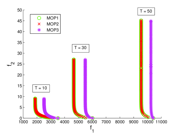
Figure 2: Trade-off curves for various periods of time.

Our study investigates optimal control strategies for different treatment periods. The trade-off curves for the treatment scenarios presented in Table 3, considering $T\in\{10,30,50\}$, are displayed in Figure 2. Overall, the larger period of study, the higher the number of individuals with AIDS and active TB. As expected, reducing the amount of control measures leads to the increase in the number of individuals with AIDS and active TB, whereas decrease in the number of individuals with AIDS and active TB can be achieved though rising expenses for treatment. These results clearly reflect the conflicting nature of the two objectives. Also, it can be seen that an efficient range of the control policies is limited, as starting from some point the reduction in the number of individuals with AIDS and active TB is possible through exponential increase in expenses for medication. Since available resources are often scarce, scenarios involving high expenses may be practically unacceptable. All curves share similar features and similar trends can be identified through analysis of the obtained solutions. Due to these facts and space limitation, in what follows the obtained results are discussed only for $T=10$.

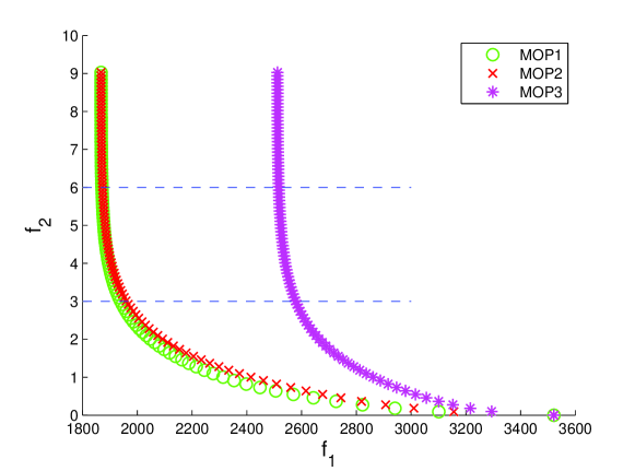
Figure 3: Trade-off curves for $T=10$.

Figure 3 shows the trade-off curves obtained for MOP1, MOP2 and MOP3, corresponding to $T=10$. As one can see, the three curves share a common point in the objective space. This represents an economic perspective, i.e., there is no treatment of TB and HIV/AIDS, the only focus is on saving money. Naturally, this leads to an uncontrollable spread of the diseases and higher numbers of individuals with AIDS and active TB. As control policies start being implemented, the response of $(A+A_{T})$ differs for the three considered cases. The best scenarios from the medical perspective, i.e., when the maximum amounts of controls are applied, are different. Interestingly, the lowest number of $(A+A_{T})$ is achieved when only implementing $u_{1}(\cdot)\equiv 0.95$, which corresponds to the treatment of patients for HIV/AIDS and TB together. In this case, scenarios resulting from MOP1 and MOP2 are identical, being represented by the same point in the objective space. However, when optimal strategies involve the treatment for TB, this allows to decrease the number of $(A+A_{T})$ in scenarios representing trade-off between the economic and medical perspectives. It can be understood observing all the intermediate solutions for MOP1 in Figure 3, which give a less value of $f_{1}$ when comparing with solutions for MOP2 involving the same amount of control measures. Though, treating patients only for TB appears to be an ineffective approach when comparing with scenarios represented by MOP1 and MOP2, as optimal solutions give significantly larger numbers of $(A+A_{T})$ along the whole Pareto optimal region.

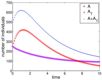
Figure 4: Dynamics of individuals with AIDS and active TB without controls.

(a) MOP1 and MOP2

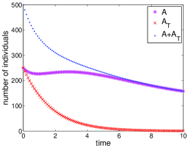
(b) MOP3

Figure 5: Dynamics of individuals with AIDS and active TB with maximum controls.

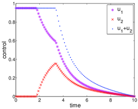
(a) MOP1

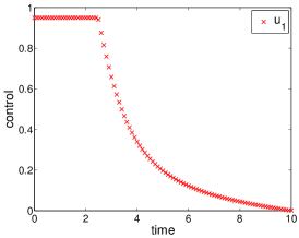
(b) MOP2

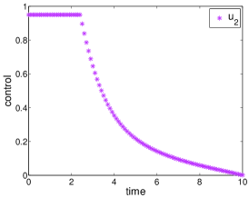
(c) MOP3

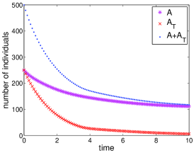
(d) MOP1

(e) MOP2

(f) MOP3

Figure 6: Controls and infected individuals for $f_{2}=3$.

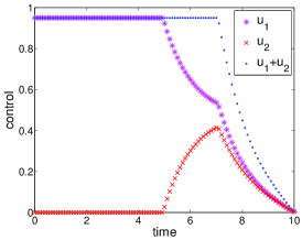
(a) MOP1

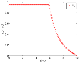
(b) MOP2

(c) MOP3

(d) MOP1

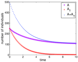
(e) MOP2

(f) MOP3

Figure 7: Controls and individuals with AIDS and active TB for $f_{2}=6$.

For the extreme solutions, i.e., those corresponding to the maximum and minimum amounts of controls applied though the period of study, the dynamics of $A$, $A_{T}$ and $(A+A_{T})$ can be observed in Figures 5 and 5. Without applying the controls, as discussed above, the corresponding dynamics are identical for MOP1, MOP2 and MOP3 and are presented in Figures 5. This scenario corresponds to the natural progression of the diseases. When only the control $u_{2}$ is applied, the number of $A$ and $A_{T}$, as well as their sum, are larger than for cases when $u_{1}$ and $u_{1}+u_{2}$ are implemented. The dynamics for $A$ and $A_{T}$ are identical for MOP1 and MOP3, which are depicted in Figure 5(a).

To analyze intermediate scenarios, two solutions lying on intermediate regions of the trade-off curves are selected. This is done as follows. The objective space is divided by two horizontal lines corresponding to $f_{2}=3$ and $f_{2}=6$ (dashed lines in Figure 3). The intersections of these lines with the trade-off curves give the three different solutions, with each of them corresponding to MOP1, MOP2 and MOP3. These solutions are selected for discussing the dynamics of the diseases. These lines can be interpreted as the constraints defining available resources for treatment. In turn, the selected solutions represent the best treatment options in such circumstances, as they allow to achieve the lowest values of $f_{1}$. It is worth noting that the solutions on different curves, shown in Figure 3, are identically distributed with respect to the values of $f_{2}$ due to the use of the $\epsilon$-constrain method. Since MOP1–3 were solved for the same values of $\epsilon$, the corresponding solutions can be used for a fair comparison. Figure 7 presents the trajectories of the control variables and the dynamics of $A$ and $A_{T}$ for solutions corresponding to $f_{2}=3$. From Figures 6(a)–6(c), it can be seen that the changes of the total amount of control measures are similar. For MOP1, the total control is composed of $u_{1}$ and $u_{2}$, which change differently during the period of study. There is a peak in $u_{2}$, taking place between the third and forth years, after which it decreases. The dynamics of $A$ and $A_{T}$ have similar trajectories, as shown in Figures 6(d)–6(f). However, there is a minor increase in $A$ for MOP3 in the beginning of the forth year. Similar trends for the control and state variables are observed in Figure 7. Though, the peak in $u_{2}$ occurs later with a higher value and the number of individuals with AIDS and active TB is lower due to the large amount of medication.

Solutions obtained using multiobjective optimization can provide comprehensive insights about the optimal strategies and the diseases dynamics resulting from implementation of those strategies. Since visual representations can help to better understand results and spot patterns that are not obvious at first, in what follows each of the variables $u_{1}$, $u_{2}$, $A$ and $A_{T}$ is defined as a function of time and the objective to which it is conflicting. By doing so, it is possible to provide the visualization of the entire optimal set of each variable. The set of optimal values defines a surface. Slicing a surface gives the trajectory of the corresponding dynamic over the period of study.

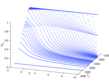
(a) $u_{1}$

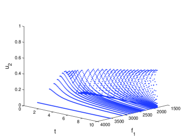
(b) $u_{2}$

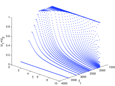
(c) $u_{1}+u_{2}$

Figure 8: Discrete representation of the optimal surface for $u_{1}$, $u_{2}$ and $u_{1}+u_{2}$.

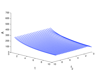
(a) $A$

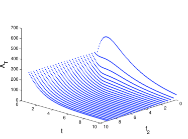
(b) $A_{T}$

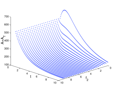
(c) $A+A_{T}$

Figure 9: Discrete representation of the optimal surface for $A$, $A_{T}$ and $A+A_{T}$.

Figure 9 shows the discrete representations of surfaces defined by the controls over the whole Pareto optimal region. On the other hand, the discrete representations of surfaces determined by the responses of $A$ and $A_{T}$ to optimal treatment strategies are illustrated in Figure 9. The plots for other classes of human population can be obtained in a similar way.

5 Conclusions

This paper investigates a mathematical model for TB-HIV/AIDS coinfection recently proposed in [25]. A multiobjective formulation is proposed. This approach avoids the use of weight parameters and allows to obtain a wide range of optimal control strategies, which offer useful information for effective decision making. Two clearly conflicting objectives are defined for search the optimal controls. The first objective reflects aspirations in controlling TB and HIV/AIDS diseases, whereas the second objective aims to reduce the costs of implementing control policies. The present study extends the previous work [25] by the extensive analysis of the optimal control in the TB-HIV/AIDS coinfection model, which enriches the knowledge about the model. Indeed, it is important not just to formulate a model but also to obtain useful information about the process modeled. Our simulation results reveal the optimal treatment strategies for TB and HIV infections and exposure to medication of different fractions of the population. This can be used as an input for planning activities to fight against TB and HIV. The choice of a final solution can be made including the goals of public healthcare and available funds. The results here obtained clearly demonstrate the usefulness and advantages of a multiobjective approach. The presence of the clearly conflicting objectives gives rise to a set of optimal solutions representing different trade-offs between them. Thus, each obtained solution reveals different perspectives on coping with AIDS and active TB diseases. The treatment of individuals infected by both HIV and TB can provide the best effects, except for the extreme scenarios. As analyses showed, the set of optimal trade-off solutions can offer to the decision maker an understanding of all possible trends in applying the controls. Moreover, the dynamics of different classes of individuals in the population appears as a response to the implemented treatment measures. The ability to obtain, analyze and choose from a set of alternatives, constitutes the major advantage of the proposed approach, motivating its practical use in the process of planning intervention measures by health authorities. As future work, we intend to study the effects of the parameters in the TB-HIV/AIDS coinfection model. Also, it would be interesting to investigate the population dynamics resulting from implementation of optimal treatment policies found by optimizing various types of objectives. Considering $L^{1}$ objectives in the optimal control problem is also the subject of future work.

References

- [1] Agusto, F.B., Adekunle, A.I.: Optimal control of a two-strain tuberculosis-HIV/AIDS co-infection model. Biosystems 119, 20–44 (2014)
- [2] Bowman Jr., V.J.: On the relationship of the Chebyshev norm and the efficient frontier of multiple criteria objectives. Lecture Notes in Economics and Mathematical Systems 130, 76–86 (1976)
- [3] Das, I., Dennis, J.E.: Normal-boundary intersection: A new method for generating the Pareto surface in nonlinear multicriteria optimization problems. SIAM Journal on Optimization 8(3), 631–657 (1998)
- [4] Deeks, S.G., Lewin, S.R., Havlir, D.V.: The end of AIDS: HIV infection as a chronic disease 382, 1525–1533 (2013)
- [5] Denysiuk, R., Rodrigues, H.S., Monteiro, M.T.T., Costa, L., Espírito Santo, I., Torres, D.F.M.: Multiobjective approach to optimal control for a dengue transmission model, Statistics, Optimization & Information Computing 3(3), 206–220 (2015) arXiv:1506.08019
- [6] Denysiuk, R., Rodrigues, H.S., Monteiro, M.T.T., Costa, L., Espírito Santo, I., Torres, D.F.M.: Dengue disease: a multiobjective viewpoint, Journal of Mathematical Analysis 7(1), 70–90 (2016) arXiv:1512.00914
- [7] Denysiuk, R., Silva, C.J., Torres, D.F.M.: Multiobjective approach to optimal control for a tuberculosis model. Optimization Methods and Software 30(5), 893–910 (2015) arXiv:1412.0528
- [8] Gass, S., Saaty, T.: The computational algorithm for the parametric objective function. Naval Research Logistics Quarterly 2(1), 39–45 (1955)
- [9] Getahun, H., Gunneberg, C., Granich, R., Nunn, P.: HIV infection-associated tuberculosis: The epidemiology and the response. Clin. Infect. Dis., 50, S201–S207 (2010)
- [10] Haimes, Y.Y., Lasdon, L.S., Wismer, D.A.: On a bicriterion formulation of the problems of integrated system identification and system optimization. IEEE Transactions on Systems, Man and Cybernetics 1(3), 296–297 (1971)
- [11] Jung, E., Lenhart, S., Feng, Z.: Optimal control of treatments in a two-strain tuberculosis model. Discrete and Continuous Dynamical Systems – Series B 2(4), 473–482 (2002)
- [12] Kirschner, D., Lenhart, S., Serbin, S.: Optimal control of the chemotherapy of HIV. J. Mathematical Biology 35, 775–792 (1996)
- [13] Lenhart, S., Workman, J.T.: Optimal control applied to biological models. Chapman & Hall/CRC, Boca Raton, FL (2007)
- [14] Magombedze, G., Mukandavire, Z., Chiyaka, C., Musuka, G.: Optimal control of a sex structured HIV/AIDS model with condom use. Mathematical Modelling and Analysis 14, 483–494 (2009)
- [15] Messac, A., Mattson, C.: Normal constraint method with guarantee of even representation of complete Pareto frontier. AIAA Journal 42, 2101–2111 (2004)
- [16] Miettinen, K.: Nonlinear multiobjective optimization, International Series in Operations Research and Management Science, vol. 12. Kluwer Academic Publishers (1999)
- [17] Morison, L.: The global epidemiology of HIV/AIDS. British Medical Bulletin 58, 7–18 (2001)
- [18] Okosun, K.O., Makinde, O.D.: A co-infection model of malaria and cholera diseases with optimal control. Mathematical Biosciences 258, 19–32 (2014)
- [19] Pascoletti, A., Serafini, P.: Scalarizing vector optimization problems. Journal of Optimization Theory and Applications 42(4), 499–524 (1984)
- [20] Pontryagin, L., Boltyanskii, V., Gramkrelidze, R., Mischenko, E.: The Mathematical Theory of Optimal Processes, 2nd edn. John Wiley (1962)
- [21] Rodrigues, P., Silva, C.J., Torres, D.F.M.: Cost-effectiveness analysis of optimal control measures for tuberculosis. Bulletin of Mathematical Biology 76(10), 2627–2645 (2014) arXiv:1409.3496
- [22] Roeger, L.W., Feng, Z., Castillo-Chavez, C.: Modeling TB and HIV co-infections. Math. Biosc. and Eng., 6, 815–837 (2009)
- [23] Rom, W.N., Markowitz, S.B.: Environmental and Occupational Medicine. Lippincott Williams & Wilkins (2007)
- [24] Silva, S.J., Torres, D.F.M.: Optimal control for a tuberculosis model with reinfection and post-exposure interventions. Mathematical Biosciences 244(2), 154–164 (2013) arXiv:1305.2145
- [25] Silva, C.J., Torres, D.F.M.: A TB-HIV/AIDS coinfection model and optimal control treatment. Discrete and Continuous Dynamical Systems – Series A 35(9), 4639–4663 (2015) arXiv:1501.03322
- [26] UNAIDS: Fact sheet 2014. Tech. Rep.
- [27] UNAIDS: Global report: UnAIDS report on the global AIDS epidemic 2013. Tech. Rep., Geneva
- [28] UNAIDS: People living with HIV. Tech. Rep., Geneva
- [29] WHO: http://www.who.int/topics/hiv_aids/en/
- [30] WHO, W.H.O.: Global tuberculosis report. WHO report, Geneva (2013)
- [31] WHO, W.H.O.: Global tuberculosis report. WHO report, Geneva (2014)
- [32] Zeleny, M.: The theory of the displaced ideal. In: M. Zeleny (ed.) Multiple Criteria Decision Making, pp. 153–206. Springer-Verlag, New York (1976)