The Faà di Bruno Hopf algebra for multivariable feedback recursions in the center problem for higher order Abel equations

Abstract

Poincaré’s center problem asks for conditions under which a planar polynomial system of ordinary differential equations has a center. It is well understood that the Abel equation naturally describes the problem in a convenient coordinate system. In 1989, Devlin described an algebraic approach for constructing sufficient conditions for a center using a linear recursion for the generating series of the solution to the Abel equation. Subsequent work by the authors linked this recursion to feedback structures in control theory and combinatorial Hopf algebras, but only for the lowest degree case. The present work introduces what turns out to be the nontrivial multivariable generalization of this connection between the center problem, feedback control, and combinatorial Hopf algebras. Once the picture is completed, it is possible to provide generalizations of some known identities involving the Abel generating series. A linear recursion for the antipode of this new Hopf algebra is also developed using coderivations. Finally, the results are used to further explore what is called the composition condition for the center problem.

MSC Classification: 34C07; 34C25; 16T05; 16T30

1 Introduction

The classical center problem first studied by Henri Poincaré Poincare_1928 considers a system of planar ordinary differential equations

$$\frac{dx}{dt}=X(x,y),\qquad\frac{dy}{dt}=Y(x,y),$$ (1)

where $X,Y$ are homogeneous polynomials with a linear part of center type. The equilibrium at the origin is a center if it is contained in an open neighborhood $U$ having no other equilibria, and every trajectory of system (1) in $U$ is closed with the same period $\omega$. The problem is usually studied in its canonical form via a reparametrization that transforms (1) into the Abel equation

$$\dot{z}(t)=v_{1}(t)z^{2}(t)+v_{2}(t)z^{3}(t),$$ (2)

where $v_{1}$ and $v_{2}$ are continuous real-valued functions Alwash-Lloyd_87 ; Cherkas_76 ; Lloyd_82 . In this setting, the origin $z=0$ is a center if $z(0)=z(\omega)=r$ for $r>0$ sufficiently small and $\omega>0$ fixed. The center problem is to determine the largest class of functions $v_{1}$ and $v_{2}$ that will render $z=0$ a center.

An algebraic approach to the center problem was first proposed by Devlin in 1989 Devlin_1989 ; Devlin_1991 , which was based on the work of Alwash and Lloyd Alwash-Lloyd_87 ; Lloyd_82 . In modern parlance, Devlin’s method was to first write the solution of the Abel equation (2) in terms of a Chen–Fliess functional expansion or Fliess operator Fliess_81 ; Fliess_83 whose coefficients are parameterized by $r$. A Fliess operator is simply a weighted sum of iterated integrals of $v_{1}$ and $v_{2}$ indexed by words in the noncommuting symbols $x_{1}$ and $x_{2}$, respectively. The concept is widely used, for example, in control theory to describe the input-output map of a system modeled in terms of ordinary differential equations. (For readers not familiar with this subject, the following references provide a good overview Fliess_81 ; Fliess_83 ; Isidori_95 ; Kawski-Sussmann_97 ; Nijmeijer-vanderSchaft_90 ; Wang-Sontag_92 ; Wang-Sontag_92a ; Wang-Sontag_95 ; Wang_90 ; Wang_95 .) Devlin showed that the generating series for his particular Fliess operator with $r=1$, which is a formal power series $c_{A}$ over words in the alphabet $X=\{x_{1},x_{2}\}$, can be decomposed as

$$c_{A}=\sum_{n=1}^{\infty}c_{A}(n),$$ (3)

where the polynomials $c_{A}(n)$, $n\geq 1$ satisfy the linear recursion

$$c_{A}(n)=(n-1)c_{A}(n-1)x_{1}+(n-2)c_{A}(n-2)x_{2},\quad n\geq 2$$ (4)

with $c_{A}(1)=1$ and $c_{A}(0)=0$. Here $\deg(x_{i}):=i$, and each letter $x_{i}$ encodes the contribution of $\nu_{i}$ to the series solution of $(\ref{Devlineq})$. His derivation used the underlying shuffle algebra induced by products of iterated integrals rather than the fact that the operator coefficients are differentially generated from the vector fields in the Abel equation (2) Fliess_81 ; Isidori_95 ; Nijmeijer-vanderSchaft_90 . Devlin also provided a recursion for the higher-order Abel equation

$$\dot{z}(t)=\sum_{i=1}^{m}v_{i}(t)z^{i+1}(t),\quad m\geq 2,$$ (5)

though the calculations become somewhat intractable. Using such recursions, it was then possible to synthesize various sufficient conditions on the $v_{i}$ under which the origin was a center. This included a generalization of the composition condition of Alwash-Lloyd_87 . The latter states that a sufficient condition for a center is the existence of a differentiable function $q$ such that $q(\omega)=q(0)$ for some $\omega>0$ and

$$v_{i}(t)=\bar{v}_{i}(q(t))\dot{q}(t),\quad i=1,\ldots,m,$$ (6)

where the $\bar{v}_{i}$ are continuous functions. For a time it was conjectured that this condition was also a necessary condition for a center if certain constraints were imposed on the $v_{i}$, for example, if they were polynomial functions of $\cos\omega t$ and $\sin\omega t$. However, a counterexample to this claim was later given by Alwash in Alwash_89 . It is still believed, however, to be a necessary condition when the $v_{i}$ are polynomials. This is now called the composition conjecture (see Alwash_09 ; Briskin-etal_10 ; Brinskin-Yomdin_05 ; Brudnyi_10 ; Yomdin_03 and the references in the survey article Gine-etal_16 ).

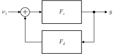
Figure 1: Feedback connection of Fliess operators $F_{c}$ and $F_{d}$

Recently, the authors revisited Devlin’s method in a combinatorial Hopf algebra setting in light of the fact that the Abel equation was found to play a central role in determining the radius of convergence of feedback connected Fliess operators as shown in Figure 1 Thitsa-Gray_12 . This recursive structure is described by the feedback equation

$$y(t)=F_{c}[\nu_{1}(t)+F_{d}[y(t)]],$$

which by a suitable choice of generating series $c$ and $d$ involving an arbitrary function $\nu_{2}(t)$ can be written directly in the form

$$\dot{z}(t) =z^{2}(t)[\nu_{1}(t)+\nu_{2}(t)y(t)]$$

$$=\nu_{1}(t)z^{2}(t)+\nu_{2}(t)z^{3}(t),$$

where $y(t)=z(t)$. It was shown in Ebrahimi-Fard-Gray_IMRN17 that the decomposition (3) is exactly the sum of the graded components of a Hopf algebra antipode applied to the formal power series $-c_{F}$, where

$$c_{F}=\sum_{k=0}^{\infty}k!\,x_{1}^{k}$$ (7)

is the Ferfera series, that is, the generating series for solution of the equation $\dot{z}=z^{2}u$, $z(0)=1$ Ferfera_79 ; Ferfera_80 . The link is made using the Hopf algebra of output feedback which encodes the composition of iterated integrals rather than their products DuffautEFG_2014 ; Gray-Duffaut_Espinosa_SCL11 ; Gray-et-al_SCL14 . As a consequence, another algebraic structure at play in Devlin’s approach beyond the shuffle algebra is a Faà di Bruno type Hopf algebra. Now it is a standard theorem that the antipode of every connected graded Hopf algebra can be computed recursively Figueroa-Gracia-Bondia_05 ; manchon2 . This fact was exploited, for example, in the authors’ application of the output feedback Hopf algebra to compute the feedback product, a device used to compute the generating series for Fliess operator representation of the interconnection shown in Figure 1 DuffautEFG_2014 ; Gray-et-al_MTNS14 . But somewhat surprisingly it was also shown in Ebrahimi-Fard-Gray_IMRN17 that for this Hopf algebra the antipode could be computed in general using a linear recursion of Devlin type. This method has been shown empirically to be more efficient than all existing methods for computing the antipode Berlin-etal_CISS17 , which is useful in control applications Duffaut_Espinosa-Gray_ACC17 ; Gray-Duffaut_Espinosa_FdB14 ; Gray-et-al_CDC15 ; Gray-et-al_Auto14 . What was not evident, however, was how all of these ideas could be related for higher order Abel equations, i.e., equation (5) when $m>2$.

The goal of this paper is to present what turns out to be the nontrivial generalization of the connection between the center problem, control theory, and combinatorial Hopf algebras for higher order Abel equations. It requires a new class of matrix-valued Fliess operators with a certain Toeplitz structure in order to provide the proper grading. In addition, a new type of multivariable output feedback Hopf algebra is needed, one which is distinct from that described in DuffautEFG_2014 ; Gray-Duffaut_Espinosa_SCL11 ; Gray-et-al_SCL14 and is more closely related to the output affine feedback Hopf algebra introduced in Gray-Ebrahimi-Fard_SIAMzz for the $m=2$ case with $v_{2}=1$ (so effectively the single-input–single-output case) to describe multiplicative output feedback. Once the picture is completed, it is possible to provide higher order extensions of some known identities for the Abel generating series, $c_{A}$. A linear recursion for the antipode of this new Hopf algebra is also developed using coderivations. Finally, a new sufficient condition for a center is given inspired by viewing the Abel equation in terms of a feedback condition. This in turn provides another way of interpreting the composition condition.

2 Linear recursions for differentially generated series and their inverses

The starting point is to show how any formal power series whose coefficients are differentially generated by a set of analytic vector fields can be written in terms of a linear recursion, as can its inverse in a certain compositional sense. This implicitly describes a group that will be utilized in the next section to describe recursions derived from feedback systems.

Consider the set of formal power series ${\mathbb{R}}\langle\langle X\rangle\rangle$ over the set of words $X^{\ast}$ generated by an alphabet of noncommuting symbols $X=\{x_{1},\ldots,x_{m}\}$. Elements of $X$ are called letters, and words over $X$ consist of finite sequences of letters, $\eta=x_{i_{1}}\cdots x_{i_{k}}\in X^{*}$. The length of a word $\eta$ is denoted $\left|\eta\right|$ and is equivalent to the number of letters it contains. When viewed as a graded vector space, where $\deg(x_{i}):=i$ and $\deg(\mathrm{e}):=0$ with $\mathrm{e}$ denoting the empty word $\emptyset\in X^{*}$, any $c\in\mbox{${\mathbb{R}}\langle\langle X\rangle\rangle$}$ can be uniquely decomposed into its homogeneous components $c=\sum_{n\geq 1}c(n)$ with $\deg(c(n))=n-1$, $n\geq 1$. In particular, if $X^{k}$ is the set of all words of length $k$, then $c(1)=\langle c,\mathrm{e}\rangle\mathrm{e}$ and

$$c(n)=\sum_{i=1}^{\min(m,n-1)}\sum_{\eta\in X^{n-1-i}}\langle c,\eta x_{i}\rangle\,\eta x_{i},\quad n\geq 2.$$ (8)

A series $c\in\mbox{${\mathbb{R}}\langle\langle X\rangle\rangle$}$ is said to be differentially generated if there exists a set of analytic vector fields $\{g_{1},g_{2},\ldots,g_{m}\}$ defined on a neighborhood $W$ of $z_{0}\in{\mathbb{R}}^{n}$ and an analytic function $h:W\to{\mathbb{R}}$ such that for every word $\eta$ in $X^{\ast}$ the corresponding coefficient of $c$ can be written as

$$\langle c,\eta\rangle=L_{g_{j_{1}}}\cdots L_{g_{j_{k}}}h(z_{0}),\quad\eta=x_{j_{k}}\cdots x_{j_{1}},$$

where the Lie derivative of $h$ with respect to $g_{j}$ is defined as the linear operator

$$L_{g_{j}}h:W\rightarrow{\mathbb{R}},\quad z\mapsto L_{g_{j}}h(z):=\frac{\partial h}{\partial z}(z)\,g_{j}(z).$$

The tuple $(g_{1},g_{2},\ldots,g_{m},z_{0},h)$ will be referred to as the generator of $c$. It follows directly that $c(n)=P_{n-1}(z_{0})$, where $P_{0}(z_{0})=h(z_{0})\mathrm{e}$ and for $n>0$, $P_{n}(z):=\sum_{\eta\in X^{n}}L_{g_{\eta}}h(z)\,\eta$, with $L_{g_{\eta}}:=L_{g_{j_{1}}}\cdots L_{g_{j_{k}}}$, and (8) can be rewritten as the linear recursion

$$P_{n}(z_{0})=\sum_{i=1}^{\min(m,n)}L_{g_{i}}P_{n-i}(z_{0})x_{i},\quad n\geq 1.$$ (9)

In this case the grading on ${\mathbb{R}}\langle\langle X\rangle\rangle$ can be encoded in the sequence $P_{n}(z_{0})$, $n\geq 1$, by assigning degrees to the vector fields, namely, $\deg(g_{i}):=\deg(x_{i})=i$, $i=1,\ldots,m$.

Example 1

Suppose $m=1$, $g_{1}(z)=z^{2}$, $z_{0}=1$, and $h(z)=z$. Then $c(1)=P_{0}(1)=h(1)\mathrm{e}=\mathrm{e}$ and

$$c(n)=P_{n-1}(1)=L_{z^{2}}P_{n-2}(1)x_{1}=(n-1)P_{n-2}(1)x_{1}=(n-1)c(n-1)x_{1},\quad n\geq 2.$$

In which case,

$$\sum_{n=1}^{\infty}c(n)=\sum_{n=1}^{\infty}(n-1)!\,x_{1}^{n-1}=\sum_{n=0}^{\infty}n!\,x_{1}^{n}=:c_{F}.$$

This is the well studied generating series of Ferfera Ferfera_79 ; Ferfera_80 .

Now suppose $d\in\mbox{${\mathbb{R}}\langle\langle X\rangle\rangle$}$ is differentially generated, and consider the corresponding Chen–Fliess series or Fliess operator

$$F_{d}[u](t):=\sum_{\eta\in X^{\ast}}\langle d,\eta\rangle\,E_{\eta}[u](t,t_{0}),$$

where $E_{\eta}[u]$ is defined inductively for each word $\eta\in X^{\ast}$ as an iterated integral over the controls $u:=(u_{1}(t),\ldots,u_{m}(t))$, $u_{i}:[t_{0},t]\rightarrow{\mathbb{R}}$, by $E_{\emptyset}[u]:=1$ and

$$E_{x_{i}\bar{\eta}}[u](t,t_{0}):=\int_{t_{0}}^{t}u_{i}(\tau)E_{\bar{\eta}}[u](\tau,t_{0})\,d\tau$$

with $x_{i}\in X$, $\bar{\eta}\in X^{\ast}$. If $u\in L_{1}^{m}[t_{0},t_{0}+T]$, that is, $u$ is measurable with finite $L_{1}$-norm, $\left\|u\right\|_{L_{1}}:=\max\{\left\|u_{i}\right\|_{1}:\ 1\leq i\leq m\}<R$, then the analyticity of the generator for $d$ is sufficient to guarantee that the Fliess operator $F_{d}[u](t)$ converges absolutely and uniformly on $[0,T]$ for sufficiently small $R,T>0$ Gray-Wang_SCL02 . Suppose next that $d=(d_{1},\ldots,d_{m-1})$ is a family of series $d_{i}\in\mbox{${\mathbb{R}}\langle\langle X\rangle\rangle$}$, $i=1,\ldots,m-1$ which are differentially generated by $(g_{1},\ldots,g_{m},z_{0},h_{1},\ldots,h_{m-1})$, and define the associated Toeplitz matrix

$$d_{{\rm{Toep}}}:=\left[\begin{array}[]{ccccc}1&d_{1}&d_{2}&\cdots&d_{m-1}\\ 0&1&d_{1}&\cdots&d_{m-2}\\ \vdots&\vdots&\vdots&\vdots&\vdots\\ 0&0&0&\cdots&d_{1}\\ 0&0&0&\cdots&1\end{array}\right]=I+\sum_{i=1}^{m-1}d_{i}N^{i},$$

where $I\in{\mathbb{R}}^{m\times m}$ is the identity matrix, and $N\in{\mathbb{R}}^{m\times m}$ is the nilpotent matrix consisting of zero entries except for a super diagonal of ones. The Toeplitz affine Fliess operator is taken to be $y=F_{d_{\delta}}[u]:=F_{d_{{\rm{Toep}}}}[u]u$, which can be written in expanded form as

$$\left[\begin{array}[]{c}y_{1}\\ y_{2}\\ \vdots\\ y_{m-1}\\ y_{m}\end{array}\right]=\left[\begin{array}[]{ccccc}1&F_{d_{1}}[u]&F_{d_{2}}[u]&\cdots&F_{d_{m-1}}[u]\\ 0&1&F_{d_{1}}[u]&\cdots&F_{d_{m-2}}[u]\\ \vdots&\vdots&\vdots&\vdots&\vdots\\ 0&0&0&\cdots&F_{d_{1}}[u]\\ 0&0&0&\cdots&1\end{array}\right]\left[\begin{array}[]{c}u_{1}\\ u_{2}\\ \vdots\\ u_{m-1}\\ u_{m}\end{array}\right].$$

Note in particular that $0_{{\rm{Toep}}}=I$ so that $F_{0_{\delta}}[u]=u$. The operator $F_{d_{\delta}}$ is realized by the analytic state space system

$$\dot{z} =\sum_{i=1}^{m}g_{i}(z)u_{i},\quad z(0)=z_{0}$$ (10a)

$$y =H(z)u,$$ (10b)

where

$$H=\left[\begin{array}[]{ccccc}1&h_{1}&h_{2}&\cdots&h_{m-1}\\ 0&1&h_{1}&\cdots&h_{m-2}\\ \vdots&\vdots&\vdots&\vdots&\vdots\\ 0&0&0&\cdots&h_{1}\\ 0&0&0&\cdots&1\end{array}\right]=I+\sum_{i=1}^{m-1}h_{i}N^{i},$$ (11)

in the sense that on some neighborhood $W$ of $z_{0}$, (10a) has a well defined solution $z(t)$ on $[t_{0},t_{0}+T]$ and $y=F_{d_{{\rm{Toep}}}}[u]u=H(z)u$ on this same interval. Since the Toeplitz matrix $H$ is always invertible and Toeplitz, it follows that the inverse operator $u=F_{d_{\delta}^{-1}}[y]:=F_{d_{{\rm{Toep}}}^{-1}}[y]y$ is another Toeplitz affine Fliess operator realized by the state space system

$$\dot{z} =\sum_{i=1}^{m}g_{i}(z)[H^{-1}(z)y]_{i},\quad z(0)=z_{0}$$ (12a)

$$u =H^{-1}(z)y.$$ (12b)

so that $F_{d_{\delta}}\circ F_{d_{\delta}^{-1}}=F_{d_{\delta}^{-1}}\circ F_{d_{\delta}}=I$. (Here $[y]_{i}$ denotes the $i$ component of $y\in{\mathbb{R}}^{m}$.) The generating series for the inverse operator, $d^{-1}=(d^{-1}_{1},\ldots,d^{-1}_{m-1})$, is differentially generated by $(\tilde{g}_{1},\ldots,\tilde{g}_{m},z_{0},\tilde{h}_{1},\ldots,\tilde{h}_{m-1})$, where $\tilde{g}_{i}:=\sum_{j=1}^{m}g_{j}H^{-1}_{ji}=g_{i}+\sum_{j=1}^{i-1}g_{i-j}\tilde{h}_{j}$ with $\tilde{h}_{j}:=H^{-1}_{1,1+j}$.

Example 2

For the case where $m=3$, system (12) becomes

$$\dot{z} =g_{1}y_{1}+(g_{2}-g_{1}h_{1})y_{2}+(g_{3}-g_{2}h_{1}+g_{1}(h_{1}^{2}-h_{2}))y_{3},\quad z(0)=z_{0}$$ (13a)

$$\left[\begin{array}[]{c}u_{1}\\ u_{2}\\ u_{3}\end{array}\right] =\left[\begin{array}[]{ccc}1&-h_{1}&h_{1}^{2}-h_{2}\\ 0&1&-h_{1}\\ 0&0&1\end{array}\right]\left[\begin{array}[]{c}y_{1}\\ y_{2}\\ y_{3}\end{array}\right].$$ (13k)

In which case,

$$F_{d_{\rm{Toep}}^{-1}}[y]=\left[\begin{array}[]{ccc}1&F_{d_{1}^{-1}}[y]&F_{d_{2}^{-1}}[y]\\ 0&1&F_{d_{1}^{-1}}[y]\\ 0&0&1\end{array}\right],$$

where $d^{-1}=(d_{1}^{-1},d_{2}^{-1})$ is generated by $(\tilde{g}_{1},\tilde{g}_{2},\tilde{g}_{3},z_{0},\tilde{h}_{1},\tilde{h}_{2})$ with $\tilde{g}_{1}:=g_{1}$, $\tilde{g}_{2}:=g_{2}-g_{1}h_{1}$, $\tilde{g}_{3}:=g_{3}-g_{2}h_{1}+g_{1}(h_{1}^{2}-h_{2})$, $\tilde{h}_{1}=-h_{1}$ and $\tilde{h}_{2}=h_{1}^{2}-h_{2}$. If coordinate functions are defined as linear maps on ${\mathbb{R}}^{2}\langle\langle X\rangle\rangle$ by

$$a^{i}_{\eta}(d):=(d_{i},\eta)=L_{g_{\eta}}h_{i}(z_{0}),\quad\eta\in X^{\ast},\;\;i=1,2,$$

and $S$ is defined as a mapping on ${\mathbb{R}}\langle X\rangle$ seen as dual space of ${\mathbb{R}}\langle\langle X\rangle\rangle$, so that

$$(S(a^{i}_{\eta}))(d):=(d_{i}^{-1},\eta)=L_{\tilde{g}_{\eta}}\tilde{h}_{i}(z_{0}),\quad\eta\in X^{\ast},\;\;i=1,2,$$

then the coordinates, i.e., coefficients of the inverse series are described compactly by the following polynomials:

$$S(a^{1}_{\mathrm{e}}) =-a^{1}_{\mathrm{e}}$$ (14a)

$$S(a^{2}_{\mathrm{e}}) =-a^{2}_{\mathrm{e}}+a^{1}_{\mathrm{e}}a^{1}_{\mathrm{e}}$$ (14b)

$$S(a^{1}_{x_{1}}) =-a^{1}_{x_{1}}$$ (14c)

$$S(a^{1}_{x_{2}}) =-a^{1}_{x_{2}}+a^{1}_{x_{1}}a^{1}_{\mathrm{e}}$$ (14d)

$$S(a^{2}_{x_{1}}) =-a^{2}_{x_{1}}+2a^{1}_{x_{1}}a^{1}_{\mathrm{e}}$$ (14e)

$$S(a^{1}_{x_{3}}) =-a^{1}_{x_{3}}+a^{1}_{x_{2}}a^{1}_{\mathrm{e}}-a^{1}_{x_{1}}a^{1}_{\mathrm{e}}a^{1}_{\mathrm{e}}+a^{1}_{x_{1}}a^{2}_{\mathrm{e}}$$ (14f)

$$S(a^{2}_{x_{2}}) =-a^{2}_{x_{2}}+2a^{1}_{x_{2}}a^{1}_{\mathrm{e}}-2a^{1}_{x_{1}}a^{1}_{\mathrm{e}}a^{1}_{\mathrm{e}}+a^{2}_{x_{1}}a^{1}_{\mathrm{e}}$$ (14g)

$$S(a^{2}_{x_{3}}) =-a^{2}_{x_{3}}+2a^{1}_{x_{3}}a^{1}_{\mathrm{e}}-2a^{1}_{x_{2}}a^{1}_{\mathrm{e}}a^{1}_{\mathrm{e}}+a^{2}_{x_{2}}a^{1}_{\mathrm{e}}-a^{2}_{x_{1}}a^{1}_{\mathrm{e}}a^{1}_{\mathrm{e}}+a^{2}_{x_{1}}a^{2}_{\mathrm{e}}+$$

$$\hskip 14.45377pt2a_{x_{1}}^{1}a_{\mathrm{e}}^{1}a_{\mathrm{e}}^{1}a_{\mathrm{e}}^{1}-2a^{1}_{x_{1}}a_{\mathrm{e}}^{1}a_{\mathrm{e}}^{2}$$ (14h)

$$\hskip 5.78172pt\vdots$$

It is not obvious in general whether the generators for the inverse series $d^{-1}_{i}$ will necessarily satisfy a linear recursion of the form (9). This is contingent on whether the new vector fields $\tilde{g}_{i}$ are consistent with the grading on ${\mathbb{R}}\langle\langle X\rangle\rangle$, that is, whether $\deg(\tilde{g}_{i})=\deg(g_{i})$, $i=1,\ldots,m$. The next theorem gives a sufficient condition under which the upper triangular Toeplitz structure of $H$ in (11) guarantees this property.

Theorem 2.1

Given any Toeplitz matrix of the form (11) and a set of vector fields $g_{i}$, $i=1,\ldots,m$ with $\deg(g_{i})=i$, it follows that $\tilde{g}_{i}:=\sum_{j=1}^{m}g_{j}H^{-1}_{ji}$ has the property $\deg(\tilde{g}_{i})=\deg(g_{i})$ provided $\deg(h_{i}):=\deg(g_{i})=i$, $i=1,\ldots,m-1$.

Proof

First observe that

$$H^{-1}=\left(I+\sum_{i=1}^{m-1}h_{i}N^{i}\right)^{-1}=\sum_{n=0}^{m-1}(-1)^{n}\left(\sum_{i=1}^{m-1}h_{i}N^{i}\right)^{n},$$

using the fact that $N^{n}=0$, $n\geq m$. Now applying the multinomial theorem gives

$$H^{-1} =I+\sum_{j=1}^{m-1}\left[\sum_{k=1}^{j}(-1)^{k}k!\sum_{k_{1}+k_{2}+\cdots+k_{j}=k\atop k_{1}+2k_{2}+\cdots+jk_{j}=j}\frac{1}{k_{1}!\cdots k_{j}!}h_{1}^{k_{1}}\cdots h_{j}^{k_{j}}\right]N^{j}.$$ (15)

$$=:I+\sum_{j=1}^{m-1}\tilde{h}_{j}N^{j}.$$

This means that $\deg(\tilde{h}_{j})=\deg(h_{1}^{k_{1}}\cdots h_{j}^{k_{j}})=k_{1}+2k_{2}+\cdots+jk_{j}=j$. Therefore, since $\tilde{g}_{i}=\sum_{j=1}^{m}g_{j}H^{-1}_{ji}=\sum_{j=0}^{i}g_{i-j}\tilde{h}_{j}$ and

$$\deg\left(g_{i-j}\tilde{h}_{j}\right)=\deg\left(g_{i-j}\right)+\deg(\tilde{h}_{j})=(i-j)+j=i,$$

it follows that $\deg(\tilde{g}_{i})=i$, $i=1,\ldots,m$ as required.

Example 3

Reconsider Example 2 in the particular case where $(g_{1},g_{2},g_{3},z_{0},h_{1},h_{2})=(z^{2},0,0,1,-z,0)$ so that $d=(-c_{F},0)$. This is an embedding of Example 1 into the case where $m=3$. The series $d^{-1}=(d_{1}^{-1},d_{2}^{-1})$ has the generator $(\tilde{g}_{1},\tilde{g}_{2},\tilde{g}_{3},z_{0},\tilde{h}_{1},\tilde{h}_{2})=(z^{2},z^{3},z^{4},1,z,z^{2})$. The system (13) reduces to the Abel system

$$\dot{z} =z^{2}y_{1}+z^{3}y_{2}+z^{4}y_{3},\quad z(0)=1$$

$$\left[\begin{array}[]{c}u_{1}\\ u_{2}\\ u_{3}\end{array}\right] =\left[\begin{array}[]{ccc}1&z&z^{2}\\ 0&1&z\\ 0&0&1\end{array}\right]\left[\begin{array}[]{c}y_{1}\\ y_{2}\\ y_{3}\end{array}\right],$$

and therefore, $c_{A,m}=d^{-1}_{1}$. Using (9) with the generator for $d_{1}^{-1}$, the Abel generating series $c_{A,3}$ can also be written as $c_{A,3}=\sum_{n\geq 1}c_{A,3}(n)$, where $c_{A,3}(1)=P_{0}(1)=\mathrm{e}$ and

$$c_{A,3}(n)=P_{n-1}(1)=L_{z^{2}}P_{n-2}(1)x_{1}+L_{z^{3}}P_{n-3}(1)x_{2}+L_{z^{4}}P_{n-4}(1)x_{3},\quad n\geq 2$$

($P_{n}(1):=0$ for $n<0$). A polynomial recursion follows from proving the identity $L_{z^{i+1}}P_{n-i-1}(1)=(n-i)P_{n-i-1}(1)$, $i=1,2,3$, so that

$$c_{A,3}(n)=(n-1)c_{A,3}(n-1)x_{1}+(n-2)c_{A,3}(n-2)x_{2}+(n-3)c_{A,3}(n-3)x_{3},\quad n\geq 2$$

($c_{A,3}(n)=0$ for $n<1$). The first few of these polynomials are:

$$c_{A,3}(1) =1$$ (16a)

$$c_{A,3}(2) =x_{1}$$ (16b)

$$c_{A,3}(3) =2x_{1}x_{1}+x_{2}$$ (16c)

$$c_{A,3}(4) =6x_{1}x_{1}x_{1}+3x_{2}x_{1}+2x_{1}x_{2}+x_{3}$$ (16d)

$$c_{A,3}(5) =24x_{1}x_{1}x_{1}x_{1}+12x_{2}x_{1}x_{1}+8x_{1}x_{2}x_{1}+4x_{3}x_{1}+6x_{1}x_{1}x_{2}+3x_{2}x_{2}+2x_{1}x_{3}.$$ (16e)

Note that each $c_{A,3}(n)$ consists only of words of degree $n-1$. These polynomials were first identified by Devlin in Devlin_1989 . The example can be generalized to any $m\geq 2$ so that

$$c_{A,m}=(I-c_{F}N)^{-1}_{1},$$ (17)

and the corresponding Abel series $c_{A,m}=\sum_{n\geq 1}c_{A,m}(n)$ can be computed from the recursion

$$c_{A,m}(n)=\sum_{i=1}^{m}(n-i)c_{A,m}(n-i)x_{i},\quad n\geq 2,$$

with $c_{A,m}(1)=1$ and $c_{A,m}(n)=0$ for $n<1$.

It is interesting to note that the construction above has some elements in common with the Faà di Bruno Hopf algebra ${\mathcal{H}}_{FdB}=(\mu,\Delta_{FdB})$ for the group $\mathcal{G}_{diff}$ of diffeomorphisms $h$ on ${\mathbb{R}}$ satisfying $h(0)=0$, $\dot{h}(0)=1$. See Figueroa-Gracia-Bondia_05 for details. First observe that (15) can also be written in terms of the Bell polynomials

$$B_{j,k}(t_{1},\ldots,t_{l}):=\sum_{k_{1}+k_{2}+\cdots+k_{l}=k\atop k_{1}+2k_{2}+\cdots+lk_{l}=j}\frac{j!}{k_{1}!\cdots k_{l}!}\left(\frac{t_{1}}{1!}\right)^{k_{1}}\cdots\left(\frac{t_{l}}{l!}\right)^{k_{l}},$$

where $l=j-k+1$, using the Faà di Bruno formula

$$f(h(t))=\sum_{j=0}^{\infty}\sum_{k=1}^{j}\beta_{k}B_{j,k}(\alpha_{1},\ldots,\alpha_{j-k+1})\frac{t^{j}}{j!}$$

with $f(t):=\sum_{n=0}^{\infty}\beta_{n}t^{n}/n!$ and $h(t)=\sum_{n=0}^{\infty}\alpha_{n}t^{n}/n!$. Specifically, setting

$$f(t) =\frac{1}{1+t}=1+\sum_{n=1}^{\infty}(-1)^{n}n!\frac{t^{n}}{n!}$$

$$h(t) =\sum_{n=1}^{m-1}n!h_{n}\frac{t^{n}}{n!}$$

gives

$$H^{-1}=f(h(N))=I+\sum_{j=1}^{m-1}\sum_{k=1}^{j}(-1)^{k}\left[\frac{k!}{j!}B_{j,k}(h_{1},2!h_{2},\ldots,(j-k+1)!h_{j-k+1})\right]N^{j}.$$

The expressions in brackets above, i.e., the ordinary Bell polynomials, are used in Brudnyi_xxBdSM to define a variation (flipped/co-opposite version) of the coproduct $\bar{\Delta}_{FdB}$ on ${\mathcal{H}}_{FdB}$ (see equations (4.1)-(4.2) in this citation). A faithful representation of the group $\mathcal{G}_{diff}$ is

$$M_{h} :=\left[\frac{k!}{j!}B_{j,k}(h_{1},2!h_{2},\ldots,(j-k+1)!h_{j-k+1})\right]^{T}$$

$$=\left[\begin{array}[]{cccccc}h_{1}&h_{2}&h_{3}&h_{4}&h_{5}&\cdots\\ 0&h_{1}^{2}&2h_{1}h_{2}&h_{2}^{2}+2h_{1}h_{3}&2h_{2}h_{3}+2h_{1}h_{4}&\cdots\\ 0&0&h_{1}^{3}&3h_{1}^{2}h_{2}&3h_{1}h_{2}^{2}+3h_{1}^{2}h_{3}&\cdots\\ 0&0&0&h_{1}^{4}&4h_{1}^{3}h_{2}&\cdots\\ 0&0&0&0&h_{1}^{5}&\cdots\\ \vdots&\vdots&\vdots&\vdots&\vdots\end{array}\right]$$

(cf. manchonfrabetti ) and

$$H^{-1}=I+\sum_{j=1}^{m-1}[{\rm\,l\!l}M_{h}]_{j}N^{j}=I+\sum_{j=1}^{m-1}\tilde{h}_{j}N^{j},$$

where ${\rm\,l\!l}:=[-1\;1\;-1\;\cdots]$. Therefore, defining the coordinate functions $a_{i}(h)=h_{i}$, $i\geq 1$, it follows that $\tilde{h}_{i}=\mu(\bar{\Delta}_{FdB}a_{i}({\rm\,l\!l},h)).$ For example,

$$\tilde{h}_{3} =\mu(\bar{\Delta}_{FdB}(a_{3})({\rm\,l\!l},h))$$

$$=\mu((a_{1}\otimes a_{3}+a_{2}\otimes 2a_{1}a_{2}+a_{3}\otimes a_{1}^{3})({\rm\,l\!l},h))$$

$$=-h_{3}+2h_{1}h_{2}-h_{1}^{3}.$$

Further observe, setting $h_{1}=1$, that the antipode $S_{FdB}$ of ${\mathcal{H}}_{FdB}$ can be identified from the top row of

$$M_{h}^{-1}=\left[\begin{array}[]{cccccc}1&-h_{2}&2h_{2}^{2}-h_{3}&-5h_{2}^{3}+5h_{2}h_{3}-h_{4}&14h_{2}^{4}-21h_{2}^{2}h_{3}+3h_{3}^{2}+6h_{2}h_{4}-h_{5}&\cdots\\ 0&1&-2h_{2}&5h_{2}^{2}-2h_{3}&-14h_{2}^{3}+12h_{2}h_{3}-2h_{4}&\cdots\\ 0&0&1&-3h_{2}&9h_{2}^{2}-3h_{3}&\cdots\\ 0&0&0&1&-4h_{2}&\cdots\\ 0&0&0&0&1&\cdots\\ \vdots&\vdots&\vdots&\vdots&\vdots\end{array}\right].$$

That is, using a standard expression for $S_{FdB}$ (see Figueroa-Gracia-Bondia_05 ), the $(j+1)th$ entry in the top row of $M_{h}^{-1}$ is given by

$$(S_{FdB}(a_{j+1}))(h) =\sum_{k=1}^{j}(-1)^{k}B_{j+k,k}(0,2!h_{2},3!h_{3},\ldots,(j+1)!h_{j+1}),\quad j\geq 1.$$

The assertion to be explored in Section 4 is that this construction has deeper connections to another kind of Faà di Bruno type Hopf algebra, one that is derived from a group of Fliess operators and used to described their feedback interconnection. In fact, the compositional inverse described above corresponds to the group inverse.

3 Devlin’s polynomials and feedback recursions

It was shown in Ebrahimi-Fard-Gray_IMRN17 that the Devlin polynomials describing the Abel generating series $c_{A,m}$ when $m=2$ can be related to a certain feedback structure commonly encountered in control theory. This in turn led to a Hopf algebra interpretation of these polynomials since feedback systems have been characterized in such terms in DuffautEFG_2014 ; Gray-Duffaut_Espinosa_SCL11 ; Gray-Duffaut_Espinosa_FdB14 ; Gray-et-al_MTNS14 ; Gray-et-al_SCL14 . In this section, the generalization of the theory is given for any $m\geq 2$. This will again provide a Hopf algebra interpretation of Devlin’s polynomials as well as a shuffle formula for the Abel series which is distinct from that derived directly from the Abel equation, namely, the non-linear recursion

$$c_{A,m}=1+\sum_{i=1}^{m}x_{i}c_{A,m}^{{\scriptscriptstyle\;\sqcup\sqcup\;}\,i+1},\quad m\geq 2,$$

where $c_{A,m}^{{\scriptscriptstyle\;\sqcup\sqcup\;}\,i}$ denotes the $i$-th shuffle power of $c_{A,m}$. Recall that ${\mathbb{R}}\langle\langle X\rangle\rangle$ consisting of all formal power series over the alphabet $X$ with coefficients in $\mathbb{R}$ forms an unital associative ${\mathbb{R}}$-algebra under the concatenation product and an unital, commutative and associative ${\mathbb{R}}$-algebra under the shuffle product, denoted here by the shuffle symbol ${\scriptscriptstyle\;\sqcup\sqcup\;}$. The latter is the ${\mathbb{R}}$-bilinear extension of the shuffle product of two words, which is defined inductively by

$$(x_{i}\eta){\scriptscriptstyle\;\sqcup\sqcup\;}(x_{j}\xi)=x_{i}(\eta{\scriptscriptstyle\;\sqcup\sqcup\;}(x_{j}\xi))+x_{j}((x_{i}\eta){\scriptscriptstyle\;\sqcup\sqcup\;}\xi)$$ (18)

with $\eta{\scriptscriptstyle\;\sqcup\sqcup\;}\emptyset=\emptyset{\scriptscriptstyle\;\sqcup\sqcup\;}\eta=\eta$ for all words $\eta,\xi\in X^{\ast}$ and letters $x_{i},x_{j}\in X$ Fliess_81 ; reutenauer . For instance, $x_{i}{\scriptscriptstyle\;\sqcup\sqcup\;}x_{j}=x_{i}x_{j}+x_{j}x_{i}$ and

$$x_{i_{1}}x_{i_{2}}{\scriptscriptstyle\;\sqcup\sqcup\;}x_{i_{3}}x_{i_{4}}=x_{i_{1}}x_{i_{2}}x_{i_{3}}x_{i_{4}}+x_{i_{3}}x_{i_{4}}x_{i_{1}}x_{i_{2}}+x_{i_{1}}x_{i_{3}}(x_{i_{2}}{\scriptscriptstyle\;\sqcup\sqcup\;}x_{i_{4}})+x_{i_{3}}x_{i_{1}}(x_{i_{2}}{\scriptscriptstyle\;\sqcup\sqcup\;}x_{i_{4}}).$$

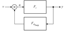
Figure 2: Multiplicative feedback system

Consider the (componentwise) multiplicative feedback interconnection shown in Figure 2 consisting of a Fliess operator $F_{c}$ in the forward path, where $c\in\mbox{${\mathbb{R}}^{m}\langle\langle X\rangle\rangle$}$, and an $m\times m$ matrix-valued Toeplitz Fliess operator $F_{d_{\rm{Toep}}}$ in the feedback path. It is useful here to define a generalized unital series, $\delta_{i}$, so that $F_{\delta_{i}}[y]:=y_{i}$ for all $i=1,\ldots,m$ and $F_{\delta_{i}^{{\scriptscriptstyle\;\sqcup\sqcup\;}j}}[y]:=(F_{\delta_{i}}[y])^{j}=y_{i}^{j}$. With $d=(\delta_{1},\delta_{1}^{{\scriptscriptstyle\;\sqcup\sqcup\;}2},\ldots,\delta_{1}^{{\scriptscriptstyle\;\sqcup\sqcup\;}m-1})$, the closed-loop system shown in Figure 2 is described by

$$y=F_{c}[u],\quad u=F_{d_{\rm{Toep}}}[y]v=v+\sum_{i=1}^{m-1}y_{1}^{i}N^{i}v,$$

and, in particular,

$$u_{1}=v_{1}+y_{1}v_{2}+y_{1}^{2}v_{3}+\cdots+y_{1}^{m-1}v_{m}.$$ (19)

Example 4

Suppose $c_{F,m}=[c_{F},0,\ldots,0]\in\mbox{${\mathbb{R}}^{m}\langle\langle X\rangle\rangle$}$, where $c_{F}=\sum_{k=0}^{\infty}k!\,x_{1}^{k}$ as in Example 1. In which case, $y_{1}=F_{c_{F}}[u]$ is realized by the one dimensional state space model

$$\dot{z}=z^{2}u_{1},\quad z(0)=1,\quad y_{1}=z.$$

Applying the feedback (19) gives the following realization for the closed-loop system

$$\dot{z}=\sum_{i=1}^{m}v_{i}z^{i+1},\quad z(0)=1,\;\;y_{1}=z,\quad i=1,\ldots,m.$$

Hence, the generating series for the closed-loop system, denoted here by $c_{F,m}@d_{\rm{Toep}}$, has the property that

$$c_{A,m}=[c_{F,m}@d_{\rm{Toep}}]_{1}.$$ (20)

This is a generalization of the result given in Ebrahimi-Fard-Gray_IMRN17 for the $m=2$ case.

In control theory, feedback is often described algebraically in terms of transformation groups. This approach is useful here as it will lead to an explicit way to compute the generating series of any closed-loop system as shown in Figure 2. Consider the group of Toeplitz affine Fliess operators

$${\mathcal{T}}:=\left\{y=F_{d_{\delta}}[u]=F_{d_{\rm{Toep}}}[u]u:d\in{\mathbb{R}}^{m-1}\langle\langle X\rangle\rangle\right\}$$

under the operator composition

$$(F_{c_{\delta}}\circ F_{d_{\delta}})[u]=F_{c_{\rm{Toep}}}[F_{d_{\rm{Toep}}}[u]u]F_{d_{\rm{Toep}}}[u]u,$$

which is associative and has the identity element $F_{0_{\delta}}$. Strictly speaking, one should limit the definition of the group to those generating series whose corresponding Fliess operators converge. But the algebraic set up presented here carries through in general if one considers the non-convergent case in a formal sense (see Gray-Wang_MTNS08 ). The group inverse has already been described for the case where $d$ is differentially generated, i.e., by equation (12). It can be shown by other arguments to exist in general (via contractive maps on ultrametric spaces, see Gray-Ebrahimi-Fard_SIAMzz ). The group product on ${\mathcal{T}}$ in turn induces a formal power series product on ${\mathbb{R}}^{m-1}\langle\langle X\rangle\rangle$ denoted by $c_{\delta}\circ d_{\delta}$ satisfying $F_{c_{\delta}\circ d_{\delta}}=F_{c_{\delta}}\circ F_{d_{\delta}}.$ Given that generating series are unique and the bijection between ${\mathbb{R}}^{m-1}\langle\langle X\rangle\rangle$ and their associated Toeplitz matrices, this means that ${\mathbb{R}}^{m-1}\langle\langle X\rangle\rangle$ inherits a group structure. A right action of the group $\mathcal{T}$ on the set of all Fliess operators $F_{c}$, $c\in\mbox{${\mathbb{R}}^{m}\langle\langle X\rangle\rangle$}$ is given by

$$(F_{c}\circ F_{d_{\delta}})[u]=F_{c}[F_{d_{\rm{Toep}}}[u]u]=F_{c}\left[u+\sum_{i=1}^{m-1}F_{d_{i}}[u]N^{i}u\right].$$

This composition induces a second formal power series product, the mixed composition product $c\>\tilde{\circ}\,d_{\delta}$, satisfying

$$F_{c}\circ F_{d_{\delta}}=F_{c\>\tilde{\circ}\,d_{\delta}}.$$ (21)

It can be viewed as a right action of the group ${\mathbb{R}}^{m-1}\langle\langle X\rangle\rangle$ on the set ${\mathbb{R}}^{m}\langle\langle X\rangle\rangle$. This product is left linear, nonassociative, and can be computed explicitly when $c\in\mbox{${\mathbb{R}}\langle\langle X\rangle\rangle$}$ by

$$c\>\tilde{\circ}\,d_{\delta}=\phi_{d}(c)(\mathbf{1})=\sum_{\eta\in X^{\ast}}\langle c,\eta\rangle\,\phi_{d}(\eta)(\mathbf{1}),$$

where $\mathbf{1}:=1\mathrm{e}$, and $\phi_{d}$ is the continuous (in the ultrametric sense) algebra homomorphism from ${\mathbb{R}}\langle\langle X\rangle\rangle$ to ${\rm End}(\mbox{${\mathbb{R}}\langle\langle X\rangle\rangle$})$ uniquely specified by $\phi_{d}(x_{i}\eta)=\phi_{d}(x_{i})\circ\phi_{d}(\eta)$ with

$$\phi_{d}(x_{i})(e)=x_{i}e+\sum_{j=1}^{m-i}x_{i+j}(d_{j}{\scriptscriptstyle\;\sqcup\sqcup\;}e),\quad i=1,\ldots,m$$ (22)

for any $e\in\mbox{${\mathbb{R}}\langle\langle X\rangle\rangle$}$, and where $\phi_{d}(\emptyset)$ denotes the identity map on ${\mathbb{R}}\langle\langle X\rangle\rangle$. For any $c\in{\mathbb{R}}^{i\times j}\langle\langle X\rangle\rangle$ the product is extended componentwise such that

$$[c\>\tilde{\circ}\,d]_{kl}=[c]_{kl}\>\tilde{\circ}\,d$$ (23)

for all $k=1,2,\ldots,i$ and $l=1,2,\ldots,j$. The following pre-Lie product results from the right linearization of the mixed composition product

$$x_{i}\eta\ \triangleleft\ d:=x_{i}(\eta\ \triangleleft\ d)+\sum_{j=1}^{m-i}x_{i+j}(d_{j}{\scriptscriptstyle\;\sqcup\sqcup\;}\eta)$$

with $\emptyset\triangleleft d:=0$. In which case, $c\>\tilde{\circ}\,d_{\delta}=c+c\triangleleft d+O(d^{2})$. In particular, it can be shown directly that

$$(c_{\delta}\circ d_{\delta})_{\rm{Toep}}=(c_{\rm{Toep}}\>\tilde{\circ}\,d_{\delta}){\scriptscriptstyle\;\sqcup\sqcup\;}d_{\rm{Toep}},$$

where the shuffle product on matrix-valued series is defined componentwise. Another useful composition product is the (unmixed) composition product $c\circ d$ induced simply by $F_{c\circ d}=F_{c}\circ F_{d}$.

With these various formal power series products defined, it is now possible to give a general formula for the feedback product $c@d_{\rm{Toep}}$ describing the generating series for the interconnected system in Figure 2. The following lemma is needed.

Lemma 1

The set $\mathcal{G}_{{\scriptscriptstyle\;\sqcup\sqcup\;}}:=\{c\in\mbox{${\mathbb{R}}^{m\times m}\langle\langle X\rangle\rangle$}:\langle c,\mathrm{e}\rangle\in Gl_{m}({\mathbb{R}})\}$ is a group under the shuffle product with the identity element being the constant series $\mathbf{I}:=I\mathrm{e}$, and the inverse of any $c\in\mathcal{G}_{{\scriptscriptstyle\;\sqcup\sqcup\;}}$ is

$$c^{{\scriptscriptstyle\;\sqcup\sqcup\;}-1}=(\langle c,\mathrm{e}\rangle(\mathbf{I}-c^{\prime}))^{{\scriptscriptstyle\;\sqcup\sqcup\;}-1}=(c^{\prime})^{{\scriptscriptstyle\;\sqcup\sqcup\;}\ast}\langle c,\mathrm{e}\rangle^{-1},$$

where $c^{\prime}$ is proper (i.e, $\langle c^{\prime},\mathrm{e}\rangle=0$), and $(c^{\prime})^{{\scriptscriptstyle\;\sqcup\sqcup\;}\ast}:=\sum_{k\geq 0}(c^{\prime})^{{\scriptscriptstyle\;\sqcup\sqcup\;}k}$.

Theorem 3.1

For any $c\in\mbox{${\mathbb{R}}^{m}\langle\langle X\rangle\rangle$}$ and $d\in\mbox{${\mathbb{R}}^{m-1}\langle\langle X\rangle\rangle$}$ it follows that $c@d_{\rm{Toep}}=c\>\tilde{\circ}\,((d_{\rm{Toep}}\circ c)^{{\scriptscriptstyle\;\sqcup\sqcup\;}-1})_{\delta}^{-1}$.

Proof

The feedback law requires that $u=F_{d_{\rm{Toep}}}[y]v=F_{d_{\rm{Toep}}}[F_{c}[u]]v=F_{d_{\rm{Toep}}\circ c}[u]v$. From Lemma 1 it follows that

$$v=F_{(d_{\rm{Toep}}\circ c)^{{\scriptscriptstyle\;\sqcup\sqcup\;}-1}}[u]u=F_{((d_{\rm{Toep}}\circ c)^{{\scriptscriptstyle\;\sqcup\sqcup\;}-1})_{\delta}}[u].$$

As the latter is now a group element in ${\mathcal{T}}$, one can write

$$u=F_{((d_{\rm{Toep}}\circ c)^{{\scriptscriptstyle\;\sqcup\sqcup\;}-1})_{\delta}^{-1}}[v].$$

Making this substitution for $u$ into $y=F_{c}[u]$ and writing the result in terms of the group action gives

$$y=F_{c@d_{\rm{Toep}}}[v]=F_{c}[F_{((d_{\rm{Toep}}\circ c)^{{\scriptscriptstyle\;\sqcup\sqcup\;}-1})_{\delta}^{-1}}[v]]=F_{c\>\tilde{\circ}\,((d_{\rm{Toep}}\circ c)^{{\scriptscriptstyle\;\sqcup\sqcup\;}-1})_{\delta}^{-1}}[v].$$

As generating series are known to be unique, the theorem is proved.

Corollary 1

The feedback product satisfies the fixed point equation $c@d_{\rm{Toep}}=c\>\tilde{\circ}\,(d_{\rm{Toep}}\circ(c@d_{\rm{Toep}}))_{\delta}$.

Proof

Observe that $y=F_{c}[F_{d_{\rm{Toep}}}[y]v]$. So if $y=F_{c@d_{\rm{Toep}}}[v]$ then necessarily

$$y=F_{c}[F_{d_{\rm{Toep}}}[F_{c@d_{\rm{Toep}}}[v]]v]=F_{c}[F_{d_{\rm{Toep}}\circ(c@d_{\rm{Toep}})}[v]v]=F_{c\>\tilde{\circ}\,(d_{\rm{Toep}}\circ(c@d_{\rm{Toep}}))_{\delta}}[v].$$

The uniqueness of generating series then proves the claim.

The tools above are now applied to compute the feedback product $c_{F,m}@d_{\rm{Toep}}$ in (20). This will in turn render identities satisfied by the Abel series. The following lemma is useful.

Lemma 2

If in (11) $h_{i}=h^{i}$, $i=1,\ldots,m-1$ for some $h\in C^{\omega}$ then $H^{-1}=I-hN$.

Proof

Given that $H=I+hN+h^{2}N^{2}+\cdots+h^{m-1}N^{m-1},$ observe

$$H^{-1} =((I-hN)^{-1}-(hN)^{m}(I-hN)^{-1})^{-1}$$

$$=(I-hN)(I-(hN)^{m})^{-1}$$

$$=I-hN+O((hN)^{m})$$

$$=I-hN,$$

since $N^{n}=0$ when $n\geq m$.

Theorem 3.2

For any $m\geq 2$, $c_{A,m}=c_{F}\>\tilde{\circ}\,(I-c_{F}N)^{-1}_{\delta}$.

Proof

Starting from the formula in Theorem 3.1 for the feedback product with $c=c_{F,m}=[c_{F},0,\ldots,0]$ and $d=(\delta_{1},\delta_{1}^{{\scriptscriptstyle\;\sqcup\sqcup\;}2},\ldots,\delta_{1}^{{\scriptscriptstyle\;\sqcup\sqcup\;}m-1})$ and using the definition of the shuffle inverse in Lemma 1, observe that

$$c_{F,m}@d_{\rm{Toep}} =c_{F,m}\>\tilde{\circ}\,((d_{\rm{Toep}}\circ c_{F,m})^{{\scriptscriptstyle\;\sqcup\sqcup\;}-1})_{\delta}^{-1}$$

$$=c_{F,m}\>\tilde{\circ}\,\left(\left(\left(I+\sum_{i=1}^{m-1}\delta_{1}^{{\scriptscriptstyle\;\sqcup\sqcup\;}i}N^{i}\right)\circ c_{F,m}\right)^{{\scriptscriptstyle\;\sqcup\sqcup\;}-1}\right)_{\delta}^{-1}$$

$$=c_{F,m}\>\tilde{\circ}\,\left(\left(\sum_{i=0}^{m-1}c_{F}^{{\scriptscriptstyle\;\sqcup\sqcup\;}i}N^{i}\right)^{{\scriptscriptstyle\;\sqcup\sqcup\;}-1}\right)_{\delta}^{-1}.$$

Now note that if $h$ in Lemma 2 is identified with $F_{c_{F}}$ then $h^{i}=F^{i}_{c_{F}}=F_{c_{F}^{{\scriptscriptstyle\;\sqcup\sqcup\;}i}}$. So the shuffle version of the identity in this lemma is $\left(\sum_{i=0}^{m-1}c_{F}^{{\scriptscriptstyle\;\sqcup\sqcup\;}i}N^{i}\right)^{{\scriptscriptstyle\;\sqcup\sqcup\;}-1}=I-c_{F}N$. In which case, $c_{F,m}@d_{\rm{Toep}}=c_{F,m}\>\tilde{\circ}\,(I-c_{F}N)_{\delta}^{-1}.$ Next, in light of (20) and (23), it is clear that $c_{A,m}=[c_{F,m}\>\tilde{\circ}\,(I-c_{F}N)_{\delta}^{-1}]_{1}=c_{F}\>\tilde{\circ}\,(I-c_{F}N)_{\delta}^{-1}$ as claimed.

Example 5

Consider evaluating $c_{A,m}=c_{F}\>\tilde{\circ}\,(I-c_{F}N)^{-1}_{\delta}$ when $m=3$. In this case

$$c_{F}\>\tilde{\circ}\,(I-c_{F}N)^{-1}_{\delta}=\sum_{k=0}^{\infty}k!\;\phi_{d}(x_{1}^{k})(\mathbf{1}),$$

where

$$\phi_{d}(x_{1})(e)=x_{1}e+x_{2}(d_{1}{\scriptscriptstyle\;\sqcup\sqcup\;}e)+x_{3}(d_{2}{\scriptscriptstyle\;\sqcup\sqcup\;}e)$$

with $d_{1}=(I-c_{F}N)^{-1}_{1}$ and $d_{2}=(I-c_{F}N)^{-1}_{2}$. Using (14) to compute the inverses gives

$$\langle d_{1},\mathrm{e}\rangle =S(a^{1}_{\mathrm{e}})(-c_{F})=-a^{1}_{\mathrm{e}}(-c_{F})=-\langle-c_{F},\mathrm{e}\rangle=1$$

$$\langle d_{1},x_{1}\rangle =S(a^{1}_{x_{1}})(-c_{F})=-a^{1}_{x_{1}}(-c_{F})=-\langle-c_{F},x_{1}\rangle=1$$

$$\langle d_{1},x_{2}\rangle =S(a^{1}_{x_{2}})(-c_{F})=(-a^{1}_{x_{2}}+a^{1}_{x_{1}}a^{1}_{\mathrm{e}})(-c_{F})$$

$$=-\langle-c_{F},x_{2}\rangle+\langle-c_{F},x_{1}\rangle\langle-c_{F},\mathrm{e}\rangle=1$$

$$\langle d_{1},x_{3}\rangle =S(a^{1}_{x_{3}})(-c_{F})=(-a^{1}_{x_{3}}+a^{1}_{x_{2}}a^{1}_{\mathrm{e}}-a^{1}_{x_{1}}a^{1}_{\mathrm{e}}a^{1}_{\mathrm{e}}+a^{1}_{x_{1}}a^{2}_{\mathrm{e}})(-c_{F})$$

$$=-\langle-c_{F},x_{3}\rangle+\langle-c_{F},x_{2}\rangle\langle-c_{F},\mathrm{e}\rangle-\langle-c_{F},x_{1}\rangle\langle-c_{F},\mathrm{e}\rangle^{2}+\langle-c_{F},x_{1}\rangle\langle 0,\mathrm{e}\rangle$$

$$=1.$$

Therefore, $d_{1}=1+x_{1}+x_{2}+x_{3}+\cdots$, which from (17) should be $c_{A,3}$. Similarly, $d_{2}=1+2x_{1}+2x_{2}+2x_{3}$, so that

$$c_{F}\>\tilde{\circ}\,(I-c_{F}N)^{-1}_{\delta} =1+x_{1}+x_{2}+x_{3}+2x_{1}x_{1}+2x_{1}x_{2}+2x_{1}x_{3}+3x_{2}x_{1}+3x_{2}x_{2}$$

$$\hskip 13.00806pt+3x_{2}x_{3}+4x_{3}x_{1}+4x_{3}x_{2}+4x_{3}x_{3}+\cdots,$$

which is also equivalent to $c_{A,3}$ as expected.

Theorem 3.3

For any $m\geq 2$

$$c_{A,m}=1+c_{A,m}{\scriptscriptstyle\;\sqcup\sqcup\;}\left(\sum_{i=1}^{m}x_{i}c_{A,m}^{{\scriptscriptstyle\;\sqcup\sqcup\;}i-1}\right).$$

Proof

Applying Corollary 1, Theorem 3.2, and the fact that the mixed composition product distributes to the left over the shuffle product gives

$$c_{A,m} =c_{F}\>\tilde{\circ}\,(d_{\rm Toep}\circ c_{A,m})_{\delta}=c_{F}\>\tilde{\circ}\,\left(\sum_{i=0}^{m}c_{A}^{{\scriptscriptstyle\;\sqcup\sqcup\;}i}N^{i}\right)_{\delta}$$

$$=\sum_{k=0}^{\infty}x_{1}^{{\scriptscriptstyle\;\sqcup\sqcup\;}k}\>\tilde{\circ}\,\left(\sum_{i=0}^{m}c_{A}^{{\scriptscriptstyle\;\sqcup\sqcup\;}i}N^{i}\right)_{\delta}=\sum_{k=0}^{\infty}\left(x_{1}\>\tilde{\circ}\,\left(\sum_{i=0}^{m}c_{A}^{{\scriptscriptstyle\;\sqcup\sqcup\;}i}N^{i}\right)_{\delta}\right)^{{\scriptscriptstyle\;\sqcup\sqcup\;}k}$$

$$=\sum_{k=0}^{\infty}\left(\sum_{i=1}^{m}x_{i}c_{A,m}^{{\scriptscriptstyle\;\sqcup\sqcup\;}i-1}\right)^{{\scriptscriptstyle\;\sqcup\sqcup\;}k}.$$

Hence, the identity in question then follows directly.

Theorem 3.3 was first observed in functional form for the $m=2$ case in Lijun-Yun_01 (see equation (2.3)). In fact, one of the main results of this paper (Theorem 4.1) is actually just a graded version of this result as described next.

Corollary 2

For any $m,n\geq 2$

$$c_{A,m}(n)=c_{A,m}(n-1){\scriptscriptstyle\;\sqcup\sqcup\;}x_{1}+\sum_{i=2}^{m}\sum_{k_{1}+\cdots+k_{i}=n-1}c_{A,m}(k_{1}){\scriptscriptstyle\;\sqcup\sqcup\;}(x_{i}(c_{A,m}(k_{2}){\scriptscriptstyle\;\sqcup\sqcup\;}\cdots c_{A,m}(k_{i}))).$$

Example 6

When $m=3$ observe $c_{A,3}=1+c_{A,3}{\scriptscriptstyle\;\sqcup\sqcup\;}(x_{1}+x_{2}c_{A,3}+x_{3}c_{A,3}^{{\scriptscriptstyle\;\sqcup\sqcup\;}2}).$ Therefore, if $a:=F_{c_{A,3}}$ then

$$a(t)=1+a(t)\left[\int_{0}^{t}u_{1}(\tau)\,d\tau+\int_{0}^{t}u_{2}(\tau)a(\tau)\,d\tau+\int_{0}^{t}u_{3}(\tau)a^{2}(\tau)\,d\tau\right].$$

Defining $a_{n}=F_{c_{A,3}(n)}$, $n\geq 1$ gives the recursion

$$a_{n}(t) =a_{n-1}(t)\int_{0}^{t}u_{1}(\tau)\,d\tau+\sum_{k_{1}+k_{2}=n-1}a_{k_{1}}(t)\int_{0}^{t}u_{2}(\tau)a_{k_{2}}(\tau)\,d\tau+$$

$$\hskip 14.45377pt\sum_{k_{1}+k_{2}+k_{3}=n-1}a_{k_{1}}(t)\int_{0}^{t}u_{3}(\tau)a_{k_{2}}(\tau)a_{k_{3}}(\tau)\,d\tau.$$

The $m=2$ case of this recursion appears in Lijun-Yun_01 as equation (1.7).

The final theorem will be generalized in Section 5 to provide a sufficient condition for a center of the Abel equation.

Theorem 3.4

Let $v_{1},v_{2},\ldots,v_{m}\in L_{1}[0,\omega]$ and $m\geq 2$ be fixed. Then the $m+1$ degree Abel equation (5) with $z(0)=1$ has the solution

$$z(t)=\frac{1}{1-E_{x_{1}}[u](t)},$$

if there exists functions $u_{1},u_{2},\ldots,u_{m}\in L_{1}[0,\omega]$ satisfying

$$v_{1}(t) =u_{1}(t)-\frac{u_{2}(t)}{1-E_{x_{1}}[u](t)}$$

$$v_{2}(t) =u_{2}(t)-\frac{u_{3}(t)}{1-E_{x_{1}}[u](t)}$$

$$\hskip 7.22743pt\vdots$$

$$v_{m-1}(t) =u_{m-1}(t)-\frac{u_{m}(t)}{1-E_{x_{1}}[u](t)}$$

$$v_{m}(t) =u_{m}(t),$$

with $E_{x_{1}}[u](t):=\int_{0}^{t}u_{1}(\tau)\,d\tau<1$ on $[0,\omega]$.

Proof

In light of Theorem 3.2, it is clear that $c_{A,m}=c_{F}\>\tilde{\circ}\,(I-c_{F}N)^{-1}_{\delta},$ and thus, $c_{F}=c_{A,m}\>\tilde{\circ}\,(I-c_{F}N)_{\delta}.$ So assume there exists $u\in L^{m}_{1}[0,\omega]$ such that

$$v=F_{(I-c_{F}N)_{\delta}}[u]=\left[\begin{array}[]{c}u_{1}-F_{c_{F}}[u]u_{2}\\ u_{2}-F_{c_{F}}[u]u_{3}\\ \vdots\\ u_{m-1}-F_{c_{F}}[u]u_{m}\\ u_{m}\end{array}\right].$$

Then, observing that $F_{c_{F}}[u]=1/(1-E_{x_{1}}[u])$, it follows from (21) that

$$z(t)=F_{c_{A,m}}[v]=F_{c_{A.m}}[F_{(I-c_{F}N)_{\delta}}[u]]=F_{c_{A,m}\>\tilde{\circ}\,(I-c_{F}N)_{\delta}}[u]=F_{c_{F}}[u]=\frac{1}{1-E_{x_{1}}[u](t)}.$$

In the next section a Hopf algebra structure is defined on the coordinate functions.

4 Multivariable Hopf algebra for Toeplitz multiplicative output feedback

All algebraic structures considered in this section are over the field $\mathbb{K}$ of characteristic zero. Let $X=\{x_{1},\ldots,x_{m}\}$ be a finite alphabet with $m$ letters. Each letter has an integer degree $\deg(x_{k}):=k$. The monoid of words is denoted by $X^{*}$ and includes the empty word $\mathrm{e}=\emptyset$ for which $\deg(\mathrm{e})=0$. The degree of a word $\eta=x_{i_{1}}\cdots x_{i_{n}}\in X^{*}$ of length $|\eta|:=n$ is defined by

$$\deg(\eta):=\sum_{k=1}^{m}k|\eta|_{k}.$$

Here $|\eta|_{k}$ denotes the number of times the letter $x_{k}\in X$ appears in the word $\eta$.

Consider the polynomial algebra $H^{(\bar{m})}$ generated by the coordinate functions $a^{k}_{\eta}$, where $\eta\in X^{*}$ and the so called root index $k\in[\bar{m}]:=\{1,\ldots,\bar{m}\}$, $\bar{m}\leq m$. By defining the degree

$$\|a^{k}_{\eta}\|:=k+\deg(\eta),$$

$H^{(\bar{m})}$ becomes a graded connected algebra, $H^{(\bar{m})}:=\bigoplus_{n\geq 0}H^{(\bar{m})}_{n}$, and $\|a^{k}_{\eta}a^{l}_{\kappa}\|=\|a^{k}_{\eta}\|+\|a^{l}_{\kappa}\|$. The unit in $H^{(\bar{m})}$ is denoted by $\mathbf{1}$, and $\|\mathbf{1}\|=0$, whereas $\|a^{k}_{\mathrm{e}}\|=k$.

The left- and right-shift maps, ${\theta}_{x_{j}}:H^{(\bar{m})}\to H^{(\bar{m})}$ respectively $\tilde{\theta}_{x_{j}}:H^{(\bar{m})}\to H^{(\bar{m})}$, for $x_{j}\in X$, are taken to be

$${\theta}_{x_{j}}a^{p}_{\eta}:=a^{p}_{x_{j}\eta},\qquad\ \tilde{\theta}_{x_{j}}a^{p}_{\eta}:={a}^{p}_{\eta x_{j}}$$

with $\theta_{x_{j}}\hbox{\bf 1}=\tilde{\theta}_{x_{j}}\hbox{\bf 1}=0$. On products in $H^{(\bar{m})}$ both these maps act as derivations

$${\theta}_{x_{j}}a^{p}_{\eta}a^{q}_{\mu}:=({\theta}_{x_{j}}a^{p}_{\eta})a^{q}_{\mu}+a^{p}_{\eta}({\theta}_{x_{j}}a^{q}_{\mu}),$$

and analogously for $\tilde{\theta}_{x_{j}}$. For a word $\eta=x_{i_{1}}\cdots x_{i_{n}}\in X^{*}$

$${\theta}_{\eta}:={\theta}_{x_{i_{1}}}\cdots{\theta}_{x_{i_{n}}},\qquad\ \tilde{\theta}_{\eta}:=\tilde{\theta}_{x_{i_{n}}}\cdots\tilde{\theta}_{x_{i_{1}}}.$$

Hence, any element $a^{i}_{\eta}\in H^{(\bar{m})}$ with $\eta=x_{i_{1}}\cdots x_{i_{n}}\in X^{*}$ can be written

$$a^{i}_{\eta}={\theta}_{\eta}a_{\mathrm{e}}^{i}=\tilde{\theta}_{\eta}a_{\mathrm{e}}^{i}.$$

In the following it will be shown how $\tilde{\theta}_{\eta}$ can be employed to define a coproduct $\Delta:H^{(\bar{m})}\to H^{(\bar{m})}\otimes H^{(\bar{m})}$. First, for the coordinate functions with respect to the empty word, $a_{\mathrm{e}}^{l}$, $1\leq l\leq\bar{m}$, the coproduct is defined to be

$$\Delta a_{\mathrm{e}}^{l}:=a_{\mathrm{e}}^{l}\otimes\hbox{\bf 1}+\hbox{\bf 1}\otimes a_{\mathrm{e}}^{l}+\sum_{k=1}^{l-1}a_{\mathrm{e}}^{k}\otimes a_{\mathrm{e}}^{l-k}.$$ (24)

Note that $a_{\mathrm{e}}^{1}$ is by definition primitive, i.e., $\Delta a_{\mathrm{e}}^{1}=a_{\mathrm{e}}^{1}\otimes\hbox{\bf 1}+\hbox{\bf 1}\otimes a_{\mathrm{e}}^{1}$. The next step is to define $\Delta$ on any $a^{i}_{\eta}$ with $1\leq i\leq\bar{m}$ and $|\eta|>0$ by specifying intertwining relations between the maps $\tilde{\theta}_{x_{i}}$ and the coproduct

$$\Delta\circ{\tilde{\theta}}_{x_{i}}:=\left(\tilde{\theta}_{x_{i}}\otimes{\rm id}+{\rm id}\otimes\tilde{\theta}_{x_{i}}+\sum_{j=1}^{i-1}\tilde{\theta}_{x_{j}}\otimes A_{\mathrm{e}}^{(i-j)}\right)\circ\Delta.$$ (25)

The map $A_{\mathrm{e}}^{(k)}$ is defined by

$$A_{\mathrm{e}}^{(k)}a^{i}_{\eta}:=a^{i}_{\eta}a_{\mathrm{e}}^{k}.$$

The following notation is used, $\Delta\circ{\tilde{\theta}}_{x_{i}}={\tilde{\Theta}}_{x_{i}}\circ\Delta$, where

$${\tilde{\Theta}}_{x_{i}}:=\tilde{\theta}_{x_{i}}\otimes{\rm id}+{\rm id}\otimes\tilde{\theta}_{x_{i}}+\sum_{j=1}^{i-1}\tilde{\theta}_{x_{j}}\otimes A_{\mathrm{e}}^{(i-j)},$$

and ${\tilde{\Theta}}_{\eta}:={\tilde{\Theta}}_{x_{i_{n}}}\cdots{\tilde{\Theta}}_{x_{i_{1}}}$ for $\eta=x_{i_{1}}\cdots x_{i_{n}}\in X^{*}$. In this setting, $a^{1}_{x_{1}}$ is primitive since

$$\Delta a^{1}_{x_{1}}=\Delta\circ{\tilde{\theta}}_{x_{1}}a^{1}_{\mathrm{e}}={\tilde{\Theta}}_{x_{1}}\circ\Delta a^{1}_{\mathrm{e}}=(\tilde{\theta}_{x_{1}}\otimes{\rm id}+{\rm id}\otimes\tilde{\theta}_{x_{1}})(a_{\mathrm{e}}^{1}\otimes\hbox{\bf 1}+\hbox{\bf 1}\otimes a_{\mathrm{e}}^{1})=a^{1}_{x_{1}}\otimes\hbox{\bf 1}+\hbox{\bf 1}\otimes a^{1}_{x_{1}},$$

which follows from $\tilde{\theta}_{x_{j}}\hbox{\bf 1}=0$. The coproduct of $a^{l}_{x_{2}}$ is

$$\Delta a^{l}_{x_{2}}=\Delta\circ\tilde{\theta}_{x_{2}}a_{\mathrm{e}}^{l}={\tilde{\Theta}}_{x_{2}}\circ\Delta a_{\mathrm{e}}^{l}=\big{(}\tilde{\theta}_{x_{2}}\otimes{\rm id}+{\rm id}\otimes\tilde{\theta}_{x_{2}}+\tilde{\theta}_{x_{1}}\otimes A_{\mathrm{e}}^{(1)}\big{)}\circ\Delta a_{\mathrm{e}}^{l}$$

$$=a^{l}_{x_{2}}\otimes\hbox{\bf 1}+\hbox{\bf 1}\otimes a^{l}_{x_{2}}+a^{l}_{x_{1}}\otimes a^{1}_{\mathrm{e}}+\sum_{k=1}^{l-1}a_{x_{2}}^{k}\otimes a_{\mathrm{e}}^{l-k}+\sum_{k=1}^{l-1}a_{\mathrm{e}}^{k}\otimes a_{x_{2}}^{l-k}+\sum_{k=1}^{l-1}a_{x_{1}}^{k}\otimes a_{\mathrm{e}}^{1}a_{\mathrm{e}}^{l-k}.$$

The coproduct of a general $a^{l}_{x_{i}}$ is

$$\Delta a^{l}_{x_{i}} =\Delta\circ\tilde{\theta}_{x_{i}}a_{\mathrm{e}}^{l}={\tilde{\Theta}}_{x_{i}}\circ\Delta a_{\mathrm{e}}^{l}=\big{(}\tilde{\theta}_{x_{i}}\otimes{\rm id}+{\rm id}\otimes\tilde{\theta}_{x_{i}}+\sum_{j=1}^{i-1}\tilde{\theta}_{x_{j}}\otimes A_{\mathrm{e}}^{(i-j)}\big{)}\circ\Delta a_{\mathrm{e}}^{l}$$

$$=a^{l}_{x_{i}}\otimes\hbox{\bf 1}+\hbox{\bf 1}\otimes a^{l}_{x_{i}}+\sum_{j=1}^{i-1}a^{l}_{x_{j}}\otimes a^{i-j}_{\mathrm{e}}+\sum_{k=1}^{l-1}a_{x_{i}}^{k}\otimes a_{\mathrm{e}}^{l-k}+\sum_{k=1}^{l-1}a_{\mathrm{e}}^{k}\otimes a_{x_{i}}^{l-k}$$

$$\hskip 14.45377pt+\sum_{j=1}^{i-1}\sum_{k=1}^{l-1}a_{x_{j}}^{k}\otimes a_{\mathrm{e}}^{i-j}a_{\mathrm{e}}^{l-k}.$$ (26)

Observe that the grading is preserved. A few examples may be helpful

$$\Delta^{\prime}a^{2}_{x_{1}} =a^{1}_{x_{1}}\otimes a^{1}_{\mathrm{e}}+a^{1}_{\mathrm{e}}\otimes a^{1}_{x_{1}}$$

$$\Delta^{\prime}a^{1}_{x_{2}} =a^{1}_{x_{1}}\otimes a^{1}_{\mathrm{e}}$$

$$\Delta^{\prime}a^{2}_{x_{2}} =a^{2}_{x_{1}}\otimes a^{1}_{\mathrm{e}}+a_{x_{2}}^{1}\otimes a_{\mathrm{e}}^{1}+a_{\mathrm{e}}^{1}\otimes a_{x_{2}}^{1}+a_{x_{1}}^{1}\otimes a_{\mathrm{e}}^{1}a_{\mathrm{e}}^{1}.$$

$$\Delta^{\prime}a^{1}_{x_{3}} =a^{1}_{x_{1}}\otimes a^{2}_{\mathrm{e}}+a^{1}_{x_{2}}\otimes a^{1}_{\mathrm{e}}$$

$$\Delta^{\prime}a^{2}_{x_{3}} =a^{2}_{x_{1}}\otimes a^{2}_{\mathrm{e}}+a^{2}_{x_{2}}\otimes a^{1}_{\mathrm{e}}+a_{x_{3}}^{1}\otimes a_{\mathrm{e}}^{1}+a_{\mathrm{e}}^{1}\otimes a_{x_{3}}^{1}+a_{x_{1}}^{1}\otimes a_{\mathrm{e}}^{2}a_{\mathrm{e}}^{1}+a_{x_{2}}^{1}\otimes a_{\mathrm{e}}^{1}a_{\mathrm{e}}^{1},$$

where $\Delta^{\prime}a^{l}_{\eta}:=\Delta a^{l}_{\eta}-a^{l}_{\eta}\otimes\hbox{\bf 1}-\hbox{\bf 1}\otimes a^{l}_{\eta}$ is the reduced coproduct. For the element $a^{l}_{x_{2}x_{1}}$ one finds the following coproduct

$$\Delta a^{l}_{x_{2}x_{1}}=\Delta\circ\tilde{\theta}_{x_{1}}\tilde{\theta}_{x_{2}}a_{\mathrm{e}}^{l}={\tilde{\Theta}}_{x_{1}}{\tilde{\Theta}}_{x_{2}}\circ\Delta a_{\mathrm{e}}^{l}$$

$$=a^{l}_{x_{2}x_{1}}\otimes\hbox{\bf 1}+\hbox{\bf 1}\otimes a^{l}_{x_{2}x_{1}}+a^{l}_{x_{1}}\otimes a^{1}_{x_{1}}+a^{l}_{x_{1}x_{1}}\otimes a^{1}_{\mathrm{e}}+\sum_{k=1}^{l-1}a_{x_{2}x_{1}}^{k}\otimes a_{\mathrm{e}}^{l-k}$$

$$+\sum_{k=1}^{l-1}a_{x_{1}}^{k}\otimes a_{x_{2}}^{l-k}+\sum_{k=1}^{l-1}a_{x_{1}x_{1}}^{k}\otimes a_{\mathrm{e}}^{1}a_{\mathrm{e}}^{l-k}+\sum_{k=1}^{l-1}a_{x_{2}}^{k}\otimes a_{x_{1}}^{l-k}+\sum_{k=1}^{l-1}a_{\mathrm{e}}^{k}\otimes a_{x_{2}x_{1}}^{l-k}$$

$$+\sum_{k=1}^{l-1}a_{x_{1}}^{k}\otimes a_{x_{1}}^{1}a_{\mathrm{e}}^{l-k}+\sum_{k=1}^{l-1}a_{x_{1}}^{k}\otimes a_{\mathrm{e}}^{1}a_{x_{1}}^{l-k}.$$

The general formula for words of length two is

$$\Delta a^{l}_{x_{j}x_{i}}=\Delta\circ\tilde{\theta}_{x_{i}}\tilde{\theta}_{x_{j}}a_{\mathrm{e}}^{l}={\tilde{\Theta}}_{x_{i}}{\tilde{\Theta}}_{x_{j}}\circ\Delta a_{\mathrm{e}}^{l}$$

$$=a^{l}_{x_{j}x_{i}}\otimes\hbox{\bf 1}+\hbox{\bf 1}\otimes a^{l}_{x_{j}x_{i}}+\sum_{n=1}^{j-1}a^{l}_{x_{n}x_{i}}\otimes a^{j-n}_{\mathrm{e}}+\sum_{n=1}^{j-1}a^{l}_{x_{n}}\otimes a^{j-n}_{x_{i}}+\sum_{s=1}^{i-1}a^{l}_{x_{j}x_{s}}\otimes a_{\mathrm{e}}^{i-s}$$

$$+\sum_{s=1}^{i-1}\sum_{n=1}^{j-1}a^{l}_{x_{n}x_{s}}\otimes a_{\mathrm{e}}^{i-s}a^{j-n}_{\mathrm{e}}+\sum_{k=1}^{l-1}a_{x_{j}x_{i}}^{k}\otimes a_{\mathrm{e}}^{l-k}+\sum_{k=1}^{l-1}a_{x_{i}}^{k}\otimes a_{x_{j}}^{l-k}+\sum_{n=1}^{j-1}\sum_{k=1}^{l-1}a_{x_{n}x_{i}}^{k}\otimes a_{\mathrm{e}}^{j-n}a_{\mathrm{e}}^{l-k}$$

$$+\sum_{k=1}^{l-1}a_{x_{j}}^{k}\otimes a_{x_{i}}^{l-k}+\sum_{k=1}^{l-1}a_{\mathrm{e}}^{k}\otimes a_{x_{j}x_{i}}^{l-k}+\sum_{n=1}^{j-1}\sum_{k=1}^{l-1}a_{x_{n}}^{k}\otimes a_{x_{i}}^{j-n}a_{\mathrm{e}}^{l-k}+\sum_{n=1}^{j-1}\sum_{k=1}^{l-1}a_{x_{n}}^{k}\otimes a_{\mathrm{e}}^{j-n}a_{x_{i}}^{l-k}$$

$$+\sum_{s=1}^{i-1}\sum_{k=1}^{l-1}a_{x_{j}x_{s}}^{k}\otimes a_{\mathrm{e}}^{i-s}a_{\mathrm{e}}^{l-k}+\sum_{s=1}^{i-1}\sum_{k=1}^{l-1}a_{x_{s}}^{k}\otimes a_{\mathrm{e}}^{i-s}a_{x_{j}}^{l-k}+\sum_{s=1}^{i-1}\sum_{n=1}^{j-1}\sum_{k=1}^{l-1}a_{x_{n}x_{s}}^{k}\otimes a_{\mathrm{e}}^{i-s}a_{\mathrm{e}}^{j-n}a_{\mathrm{e}}^{l-k}.$$

The coproduct is then extended multiplicatively to all of $H^{(\bar{m})}$ and $\Delta(\hbox{\bf 1}):=\hbox{\bf 1}\otimes\hbox{\bf 1}$.

Theorem 4.1

$H^{(\bar{m})}$ is a connected graded commutative non-cocommutative Hopf algebra with unit map $u:\mathbb{K}\to H^{(\bar{m})}$, counit $\epsilon:H^{(\bar{m})}\to\mathbb{K}$ and coproduct $\Delta:H^{(\bar{m})}\to H^{(\bar{m})}\otimes H^{(\bar{m})}$

$$\Delta a_{\eta}^{k}={\tilde{\Theta}}_{\eta}\circ\Delta a^{k}_{\mathrm{e}}.$$ (27)

Proof

$H^{(\bar{m})}=\bigoplus_{n\geq 0}H_{n}^{(\bar{m})}$ is connected graded and commutative by construction. In addition, it is clear that the coproduct is non-cocommutative. What is left to be shown is coassociativity. This is done by first proving the claim for $a_{\mathrm{e}}^{l}$, which follows from the identity

$$\sum_{k=1}^{l-1}\sum_{p=1}^{k-1}a_{\mathrm{e}}^{p}\otimes a_{\mathrm{e}}^{k-p}\otimes a_{\mathrm{e}}^{l-k}=\sum_{k=1}^{l-1}\sum_{p=1}^{l-k-1}a_{\mathrm{e}}^{k}\otimes a_{\mathrm{e}}^{p}\otimes a_{\mathrm{e}}^{l-k-p}.$$

From $\Delta(a_{\eta x_{i}}^{k})=\Delta\circ\tilde{\theta}_{x_{i}}(a_{\eta}^{k})=\tilde{\Theta}_{x_{i}}\circ\Delta(a_{\eta}^{k})$ it follows that

$$(\Delta\otimes{\rm id})\circ\Delta(a_{\eta x_{i}}^{k})=(\Delta\otimes{\rm id})\circ\tilde{\Theta}_{x_{i}}\circ\Delta(a_{\eta}^{k})$$

$$=\Big{(}\Delta\circ\tilde{\theta}_{x_{i}}\otimes{\rm id}+{\rm id}\otimes{\rm id}\otimes\tilde{\theta}_{x_{i}}+\sum_{j=1}^{i-1}\Delta\circ\tilde{\theta}_{x_{j}}\otimes A_{\mathrm{e}}^{(i-j)}\Big{)}\circ\Delta(a_{\eta}^{k})$$

$$=\Big{(}\tilde{\Theta}_{x_{i}}\otimes{\rm id}+{\rm id}\otimes{\rm id}\otimes\tilde{\theta}_{x_{i}}+\sum_{j=1}^{i-1}\tilde{\Theta}_{x_{j}}\otimes A_{\mathrm{e}}^{(i-j)}\Big{)}(\Delta\otimes{\rm id})\circ\Delta(a_{\eta}^{k})$$

$$=\Big{(}\tilde{\theta}_{x_{i}}\otimes{\rm id}\otimes{\rm id}+{\rm id}\otimes\tilde{\theta}_{x_{i}}\otimes{\rm id}+{\rm id}\otimes{\rm id}\otimes\tilde{\theta}_{x_{i}}$$

$$+\sum_{j=1}^{i-1}\tilde{\theta}_{x_{j}}\otimes A_{\mathrm{e}}^{(i-j)}\otimes{\rm id}+\sum_{j=1}^{i-1}\tilde{\theta}_{x_{j}}\otimes{\rm id}\otimes A_{\mathrm{e}}^{(i-j)}$$

$$+\sum_{j=1}^{i-1}{\rm id}\otimes\tilde{\theta}_{x_{j}}\otimes A_{\mathrm{e}}^{(i-j)}+\sum_{j=1}^{i-1}\sum_{k=1}^{j-1}\tilde{\theta}_{x_{k}}\otimes A_{\mathrm{e}}^{(j-k)}\otimes A_{\mathrm{e}}^{(i-j)}\Big{)}({\rm id}\otimes\Delta)\circ\Delta(a_{\eta}^{k})$$

$$=\Big{(}\tilde{\theta}_{x_{i}}\otimes{\rm id}\otimes{\rm id}+{\rm id}\otimes\tilde{\Theta}_{x_{i}}+\sum_{j=1}^{i-1}\tilde{\theta}_{x_{j}}\otimes\Big{(}A_{\mathrm{e}}^{(i-j)}\otimes{\rm id}+{\rm id}\otimes A_{\mathrm{e}}^{(i-j)}\Big{)}$$

$$+\sum_{j=1}^{i-1}\sum_{k=1}^{j-1}\tilde{\theta}_{x_{k}}\otimes A_{\mathrm{e}}^{(j-k)}\otimes A_{\mathrm{e}}^{(i-j)}\Big{)}({\rm id}\otimes\Delta)\circ\Delta(a_{\eta}^{k}).$$

As noted above, the last sum can be rewritten as

$$\sum_{j=1}^{i-1}\sum_{k=1}^{j-1}\tilde{\theta}_{x_{k}}\otimes A_{\mathrm{e}}^{(j-k)}\otimes A_{\mathrm{e}}^{(i-j)}=\sum_{j=1}^{i-2}\sum_{k=1}^{i-j-1}\tilde{\theta}_{x_{j}}\otimes A_{\mathrm{e}}^{(k)}\otimes A_{\mathrm{e}}^{(i-j-k)}$$

so that

$$\Big{(}\tilde{\theta}_{x_{i}}\otimes{\rm id}\otimes{\rm id}+{\rm id}\otimes\tilde{\Theta}_{x_{i}}+\sum_{j=1}^{i-1}\tilde{\theta}_{x_{j}}\otimes\big{(}A_{\mathrm{e}}^{(i-j)}\otimes{\rm id}+{\rm id}\otimes A_{\mathrm{e}}^{(i-j)}\big{)}$$

$$+\sum_{j=1}^{i-1}\sum_{k=1}^{j-1}\tilde{\theta}_{x_{k}}\otimes A_{\mathrm{e}}^{(j-k)}\otimes A_{\mathrm{e}}^{(i-j)}\Big{)}({\rm id}\otimes\Delta)\circ\Delta(a_{\eta}^{k})$$

$$=\Big{(}\tilde{\theta}_{x_{i}}\otimes{\rm id}\otimes{\rm id}+{\rm id}\otimes\tilde{\Theta}_{x_{i}}$$

$$+\sum_{j=1}^{i-1}\tilde{\theta}_{x_{j}}\otimes\Big{(}A_{\mathrm{e}}^{(i-j)}\otimes{\rm id}+{\rm id}\otimes A_{\mathrm{e}}^{(i-j)}+\sum_{k=1}^{i-j-1}A_{\mathrm{e}}^{(k)}\otimes A_{\mathrm{e}}^{(i-j-k)}\Big{)}\Big{)}({\rm id}\otimes\Delta)\circ\Delta(a_{\eta}^{k})$$

$$=({\rm id}\otimes\Delta)\circ\Big{(}\tilde{\theta}_{x_{i}}\otimes{\rm id}+{\rm id}\otimes\tilde{\theta}_{x_{i}}+\sum_{j=1}^{i-1}\tilde{\theta}_{x_{j}}\otimes A_{\mathrm{e}}^{(i-j)}\Big{)}\circ\Delta(a_{\eta}^{k})$$

$$=({\rm id}\otimes\Delta)\circ\Delta(a_{\eta x_{i}}^{k}).$$

The following was also used in the calculation above

$$\Delta\circ A_{\mathrm{e}}^{(i-j)}=\Big{(}A_{\mathrm{e}}^{(i-j)}\otimes{\rm id}+{\rm id}\otimes A_{\mathrm{e}}^{(i-j)}+\sum_{k=1}^{i-j-1}A_{\mathrm{e}}^{(k)}\otimes A_{\mathrm{e}}^{(i-j-k)}\Big{)}\circ\Delta,$$

which follows from $A_{\mathrm{e}}^{(l)}a_{\eta}^{k}=a_{\mathrm{e}}^{l}a_{\eta}^{k}$ together with the multiplicativity of $\Delta$.

In the following, a variant of Sweedler’s notation Sweedler_69 is used for the reduced coproduct, i.e., $\Delta^{\prime}(a^{l}_{\eta})=\sum a^{l^{\prime}}_{\eta^{\prime}}\otimes a^{l^{\prime\prime}}_{\eta^{\prime\prime}}$, as well as for the full coproduct

$$\Delta(a^{l}_{\eta})=\sum a^{l^{\prime}}_{\eta_{(1)}}\otimes a^{l^{\prime\prime}}_{\eta_{(2)}}=a^{l}_{\eta}\otimes{\bf{1}}+{\bf{1}}\otimes a^{l}_{\eta}+\Delta^{\prime}(a^{l}_{\eta}).$$

Connectedness of $H^{(\bar{m})}$ implies for the antipode $S:H^{(\bar{m})}\to H^{(\bar{m})}$ the well known recursions

$$Sa^{l}_{\eta}=-a^{l}_{\eta}-\sum S(a^{l^{\prime}}_{\eta^{\prime}})a^{l^{\prime\prime}}_{\eta^{\prime\prime}}=-a^{l}_{\eta}-\sum a^{l^{\prime}}_{\eta^{\prime}}S(a^{l^{\prime\prime}}_{\eta^{\prime\prime}}).$$ (28)

A few examples are given first. Coproduct (24) implies for the elements $a^{k}_{\mathrm{e}}$ that

$$Sa^{k}_{\mathrm{e}}=-a^{k}_{\mathrm{e}}+\sum_{i=2}^{k}(-1)^{i}\sum_{p_{1}+\cdots+p_{i}=k\atop p_{j}>0}a^{p_{1}}_{\mathrm{e}}\cdots a^{p_{i}}_{\mathrm{e}}.$$ (29)

For example,

$$Sa^{1}_{\mathrm{e}}=-a^{1}_{\mathrm{e}},\qquad Sa^{2}_{\mathrm{e}}=-a^{2}_{\mathrm{e}}+a^{1}_{\mathrm{e}}a^{1}_{\mathrm{e}},\qquad Sa^{3}_{\mathrm{e}}=-a^{3}_{\mathrm{e}}+2a^{1}_{\mathrm{e}}a^{2}_{\mathrm{e}}-a^{1}_{\mathrm{e}}a^{1}_{\mathrm{e}}a^{1}_{\mathrm{e}}.$$

The following examples are given for comparison with (14):

$$Sa^{1}_{x_{1}} =-a^{1}_{x_{1}}$$

$$Sa^{1}_{x_{2}} =-a^{1}_{x_{2}}+a^{1}_{x_{1}}a^{1}_{\mathrm{e}}$$

$$Sa^{1}_{x_{3}} =-a^{1}_{x_{3}}+a^{1}_{x_{1}}a^{2}_{\mathrm{e}}-a^{1}_{x_{1}}a^{1}_{\mathrm{e}}a^{1}_{\mathrm{e}}+a^{1}_{x_{2}}a^{1}_{\mathrm{e}}$$

$$Sa^{2}_{x_{1}} =-a^{2}_{x_{1}}+2a^{1}_{x_{1}}a^{1}_{\mathrm{e}}$$

$$Sa^{2}_{x_{2}} =-a^{2}_{x_{2}}+a^{2}_{x_{1}}a^{1}_{\mathrm{e}}-2a^{1}_{x_{1}}a^{1}_{\mathrm{e}}a^{1}_{\mathrm{e}}+2a^{1}_{x_{2}}a^{1}_{\mathrm{e}}$$

$$Sa^{2}_{x_{3}} =-a^{2}_{x_{3}}+2a^{1}_{x_{3}}a^{1}_{\mathrm{e}}-2a^{1}_{x_{2}}a^{1}_{\mathrm{e}}a^{1}_{\mathrm{e}}+a^{2}_{x_{2}}a^{1}_{\mathrm{e}}-a^{2}_{x_{1}}a^{1}_{\mathrm{e}}a^{1}_{\mathrm{e}}+a^{2}_{x_{1}}a^{2}_{\mathrm{e}}$$

$$\hskip 14.45377pt-2a^{1}_{x_{1}}a^{1}_{\mathrm{e}}a^{2}_{\mathrm{e}}+2a^{1}_{x_{1}}a^{1}_{\mathrm{e}}a^{1}_{\mathrm{e}}a^{1}_{\mathrm{e}}$$

The next theorem uses the coproduct formula (25) to provide a simple formula for the antipode of $H^{(\bar{m})}$.

Theorem 4.2

For any nonempty word $\eta=x_{i_{1}}\cdots x_{i_{l}}\in X^{\ast}$, the antipode $S:H^{(\bar{m})}\to H^{(\bar{m})}$ can be written as

$$Sa^{k}_{\eta}=\tilde{\Theta}^{\prime}_{\eta}(Sa^{k}_{\mathrm{e}}),$$ (30)

where $\tilde{\Theta}^{\prime}_{\eta}:=\tilde{\theta}^{\prime}_{x_{i_{l}}}\circ\cdots\circ\tilde{\theta}^{\prime}_{x_{i_{1}}}$ with

$$\tilde{\theta}^{\prime}_{x_{l}} :=\tilde{\theta}_{x_{l}}+\sum_{j=1}^{l-1}S(a_{\mathrm{e}}^{l-j})\tilde{\theta}_{x_{j}}.$$

For instance, calculating

$$\tilde{\Theta}^{\prime}_{x_{1}}(Sa^{3}_{\mathrm{e}}) =\tilde{\theta}_{x_{1}}(-a^{3}_{\mathrm{e}}+2a^{1}_{\mathrm{e}}a^{2}_{\mathrm{e}}-a^{1}_{\mathrm{e}}a^{1}_{\mathrm{e}}a^{1}_{\mathrm{e}})=-a^{3}_{x_{1}}+2a^{1}_{x_{1}}a^{2}_{\mathrm{e}}+2a^{1}_{\mathrm{e}}a^{2}_{x_{1}}-3a^{1}_{x_{1}}a^{1}_{\mathrm{e}}a^{1}_{\mathrm{e}},$$

which coincides with $Sa^{3}_{x_{1}}$. Another example is

$$\tilde{\Theta}^{\prime}_{x_{2}}(Sa^{2}_{\mathrm{e}})=(\tilde{\theta}_{x_{2}}+S(a_{\mathrm{e}}^{1})\tilde{\theta}_{x_{1}})(-a^{2}_{\mathrm{e}}+a^{1}_{\mathrm{e}}a^{1}_{\mathrm{e}})=-a^{2}_{x_{2}}+2a^{1}_{x_{2}}a^{1}_{\mathrm{e}}+a^{2}_{x_{1}}a^{1}_{\mathrm{e}}-2a^{1}_{x_{1}}a^{1}_{\mathrm{e}}a^{1}_{\mathrm{e}}.$$

Proof

The proof follows by a nested induction using the weight of the root index and word length. First, formula (30) is shown to hold for words of length one. Note that the recursions (28) can be written in terms of the convolution product, i.e., $-S=P*S=S*P$, which is defined in terms of the coproduct (27)

$$S=-m_{H^{(\bar{m})}}\circ\big{(}P\otimes S\big{)}\circ\Delta=-m_{H^{(\bar{m})}}\circ\big{(}S\otimes P\big{)}\circ\Delta.$$

Here $m_{H^{(\bar{m})}}$ denotes the product in $H^{(\bar{m})}$ and $P:={\rm id}-u\circ\epsilon$ is the projector that maps the unit 1 in ${H^{(\bar{m})}}$ to zero and reduces to the identity on $H_{+}^{(\bar{m})}=\bigoplus_{n>0}H_{n}^{(\bar{m})}$. Formula (30) applied to $a^{1}_{x_{l}}$ gives

$$\tilde{\Theta}^{\prime}_{x_{l}}(Sa^{1}_{\mathrm{e}})=\Big{(}\tilde{\theta}_{x_{l}}+\sum_{j=1}^{l-1}S(a_{\mathrm{e}}^{l-j})\tilde{\theta}_{x_{j}}\Big{)}Sa^{1}_{\mathrm{e}}=-a^{1}_{x_{l}}-\sum_{j=1}^{l-1}S(a_{\mathrm{e}}^{l-j})a^{1}_{x_{j}},$$

where (29) was used. This coincides with

$$Sa^{1}_{x_{l}} =-m_{H^{(\bar{m})}}\circ\big{(}P\otimes S\big{)}\circ\Delta a^{1}_{x_{l}}$$

$$=-m_{H^{(\bar{m})}}\circ\big{(}P\otimes S\big{)}\Big{(}a^{1}_{x_{l}}\otimes\hbox{\bf 1}+\hbox{\bf 1}\otimes a^{1}_{x_{l}}+\sum_{j=1}^{l-1}a^{1}_{x_{j}}\otimes a^{l-j}_{\mathrm{e}}\Big{)}$$

$$=-a^{1}_{x_{l}}-\sum_{j=1}^{l-1}S(a_{\mathrm{e}}^{l-j})a^{1}_{x_{j}}.$$

Now (30) applied to $a^{k}_{x_{l}}$ gives

$$\tilde{\Theta}^{\prime}_{x_{l}}(Sa^{k}_{\mathrm{e}}) =\Big{(}\tilde{\theta}_{x_{l}}+\sum_{j=1}^{l-1}S(a_{\mathrm{e}}^{l-j})\tilde{\theta}_{x_{j}}\Big{)}Sa^{k}_{\mathrm{e}}$$

$$=\Big{(}\tilde{\theta}_{x_{l}}+\sum_{j=1}^{l-1}S(a_{\mathrm{e}}^{l-j})\tilde{\theta}_{x_{j}}\Big{)}\Big{(}-a^{k}_{\mathrm{e}}-\sum_{w=1}^{k-1}a^{w}_{\mathrm{e}}Sa^{k-w}_{\mathrm{e}}\Big{)}$$

$$=-a^{k}_{x_{l}}-\sum_{j=1}^{l-1}S(a_{\mathrm{e}}^{l-j})a^{k}_{x_{j}}-\sum_{w=1}^{k-1}a^{w}_{x_{l}}Sa^{k-w}_{\mathrm{e}}-\sum_{j=1}^{l-1}\sum_{w=1}^{k-1}a^{w}_{x_{j}}S(a_{\mathrm{e}}^{l-j})S(a^{k-w}_{\mathrm{e}})$$

$$\hskip 14.45377pt-\sum_{w=1}^{k-1}a^{w}_{\mathrm{e}}\tilde{\Theta}^{\prime}_{x_{l}}Sa^{k-w}_{\mathrm{e}}.$$

Using the induction hypothesis on the last term, namely, $\tilde{\Theta}^{\prime}_{x_{l}}Sa^{k-w}_{\mathrm{e}}=Sa^{k-w}_{x_{l}}$, gives

$$\tilde{\Theta}^{\prime}_{x_{l}}(Sa^{k}_{\mathrm{e}}) =-a^{k}_{x_{l}}-\sum_{j=1}^{l-1}S(a_{\mathrm{e}}^{l-j})a^{k}_{x_{j}}-\sum_{w=1}^{k-1}a^{w}_{x_{l}}Sa^{k-w}_{\mathrm{e}}-\sum_{j=1}^{l-1}\sum_{w=1}^{k-1}a^{w}_{x_{j}}S(a_{\mathrm{e}}^{l-j})S(a^{k-w}_{\mathrm{e}})$$

$$\hskip 14.45377pt-\sum_{w=1}^{k-1}a^{w}_{\mathrm{e}}Sa^{k-w}_{x_{l}}.$$

This coincides with the antipode computed via the coproduct in (26) since

$$Sa^{k}_{x_{l}} =-m_{H^{(\bar{m})}}\circ\big{(}P\otimes S\big{)}\circ\Delta a^{k}_{x_{l}}$$

$$=-m_{H^{(\bar{m})}}\circ\big{(}P\otimes S\big{)}\Big{(}a^{k}_{x_{l}}\otimes\hbox{\bf 1}+\hbox{\bf 1}\otimes a^{k}_{x_{l}}+\sum_{j=1}^{l-1}a^{k}_{x_{j}}\otimes a^{l-j}_{\mathrm{e}}$$

$$\hskip 14.45377pt+\sum_{w=1}^{k-1}a_{x_{l}}^{w}\otimes a_{\mathrm{e}}^{k-w}+\sum_{j=1}^{l-1}\sum_{w=1}^{k-1}a_{x_{j}}^{w}\otimes a_{\mathrm{e}}^{l-j}a_{\mathrm{e}}^{k-w}+\sum_{w=1}^{k-1}a_{\mathrm{e}}^{w}\otimes a_{x_{l}}^{k-w}\Big{)}.$$

Now suppose (30) holds for all words $\nu\in X^{*}$ up to length $|\nu|=n-1$. The final step is to consider $a^{l}_{\eta}$, where $\eta=x_{i_{1}}\cdots x_{i_{n}}=\bar{\eta}x_{i_{n}}$, i.e., $|\eta|=n$, and $l\in[\bar{m}]$. Observe

$$\tilde{\Theta}^{\prime}_{\eta}(a^{l}_{\mathrm{e}}) =\tilde{\Theta}^{\prime}_{x_{i_{n}}}S(a^{l}_{\bar{\eta}})$$

$$=-\tilde{\Theta}^{\prime}_{x_{i_{n}}}m_{H^{(\bar{m})}}\circ\big{(}P\otimes S\big{)}\circ\Delta a^{l}_{\bar{\eta}}$$

$$=-m_{H^{(\bar{m})}}\circ\big{(}(\tilde{\Theta}^{\prime}_{x_{i_{n}}}\otimes{\rm id}+{\rm id}\otimes\tilde{\Theta}^{\prime}_{x_{i_{n}}})\circ(P\otimes S)\big{)}\circ\Delta a^{l}_{\bar{\eta}}$$

$$=-m_{H^{(\bar{m})}}\circ\big{(}P\circ\tilde{\Theta}^{\prime}_{x_{i_{n}}}\otimes S+P\otimes\tilde{\Theta}^{\prime}_{x_{i_{n}}}\circ S\big{)}\circ\Delta a^{l}_{\bar{\eta}}$$

$$=-m_{H^{(\bar{m})}}\circ\Big{(}P\circ\tilde{\theta}_{x_{i_{n}}}\otimes S+P\circ\sum_{j=1}^{i_{n}-1}S(a_{\mathrm{e}}^{i_{n}-j})\tilde{\theta}_{x_{j}}\otimes S+P\otimes S\circ\tilde{\theta}_{x_{i_{n}}}\Big{)}\circ\Delta a^{l}_{\bar{\eta}}$$

$$=-m_{H^{(\bar{m})}}\circ\Big{(}(P\otimes S)\circ\big{(}\tilde{\theta}_{x_{i_{n}}}\otimes{\rm id}+\sum_{j=1}^{i_{n}-1}\tilde{\theta}_{x_{j}}\otimes A_{\mathrm{e}}^{(i_{n}-j)}+{\rm id}\otimes\tilde{\theta}_{x_{i_{n}}}\big{)}\Big{)}\circ\Delta a^{l}_{\bar{\eta}}$$

$$=-m_{H^{(\bar{m})}}\circ\big{(}P\otimes S\big{)}\circ\tilde{\Theta}_{x_{i_{n}}}\circ\Delta a^{l}_{\bar{\eta}}$$

$$=-m_{H^{(\bar{m})}}\circ\big{(}P\otimes S\big{)}\circ\Delta a^{l}_{\eta}=Sa^{l}_{\eta}.$$

The third equality above came from that fact the $\tilde{\Theta}^{\prime}_{x_{i_{n}}}$ is a sum of derivations. The fourth equality is a consequence of the identity $P\circ\tilde{\theta}_{x_{i_{n}}}=\tilde{\theta}_{x_{i_{n}}}\circ P$. The step from the fourth to the fifth equality used the induction hypothesis to get $P\otimes\tilde{\Theta}^{\prime}_{x_{i_{n}}}\circ S=P\otimes S\circ\tilde{\theta}_{x_{i_{n}}}$, which holds due to the projector $P$ being on the left-hand side. In addition, the following identity was used:

$$m_{H^{(\bar{m})}}\circ\Big{(}P\circ\sum_{j=1}^{i_{n}-1}S(a_{\mathrm{e}}^{i_{n}-j})\tilde{\theta}_{x_{j}}\otimes S\Big{)}\circ\Delta=m_{H^{(\bar{m})}}\circ\Big{(}(P\otimes S)\circ\sum_{j=1}^{i_{n}-1}\tilde{\theta}_{x_{j}}\otimes A_{\mathrm{e}}^{(i_{n}-j)}\Big{)}\circ\Delta,$$

which holds due to $S$ being an algebra morphism.

The final result is evident from the fact that the feedback structures in Figures 1 and 2 coincide when condition (19) holds with $m=2$.

Corollary 3

For the alphabet $X:=\{x_{1},x_{2}\}$ the Hopf algebra $H^{(1)}$ coincides with the Faà di Bruno-type Hopf algebra for single-input, single-output (SISO) output feedback given in Foissy_13 ; Gray-Duffaut_Espinosa_SCL11 ; Gray-Duffaut_Espinosa_FdB14 .

5 Sufficient condition for a center of the Abel equation

Consider first a new sufficient condition for a center inspired by viewing the Abel equation in terms of a feedback connection as described in Section 3.

Theorem 5.1

Let $v_{1},v_{2},\ldots,v_{m}\in L_{1}[0,\omega]$ and $m\geq 2$ be fixed. Then the $m+1$ degree Abel equation (5) has a center at $z=0$ if there exists an $R>0$ such that for every $r<R$ the system of equations

$$v_{1}(t) =u_{1}(t)-\frac{ru_{2}(t)}{1-rE_{x_{1}}[u](t)}$$ (31a)

$$v_{2}(t) =u_{2}(t)-\frac{ru_{3}(t)}{1-rE_{x_{1}}[u](t)}$$ (31b)

$$\hskip 7.22743pt\vdots$$

$$v_{m-1}(t) =u_{m-1}(t)-\frac{ru_{m}(t)}{1-rE_{x_{1}}[u](t)}$$ (31c)

$$v_{m}(t) =u_{m}(t),$$ (31d)

has a solution $u_{1},u_{2},\ldots,u_{m}\in L_{1}[0,\omega]$ with $E_{x_{1}}[u](t):=\int_{0}^{t}u_{1}(\tau)\,d\tau<1/r$ on the interval $[0,\omega]$ and $E_{x_{1}}[u](\omega)=0$.

Proof

The claim is proved by showing that if the system (31) has the solution $u_{1}$, $u_{2}$,…, $u_{m}$ then the Abel equation (5) with $z(0)=r<R$ has the solution

$$z(t)=\frac{r}{1-rE_{x_{1}}[u](t)}.$$ (32)

In which case, $z(0)=z(\omega)=r$ for all $r<R$ so that $z=0$ is a center.

Consider the case where $m=2$ for simplicity. The proposed solution for (5) can be checked by direct substitution. That is,

$$\dot{z}(t)=\frac{r^{2}}{\left(1-rE_{x_{1}}[u](t)\right)^{2}}u_{1}(t),$$

so that

$$v_{1}(t)z^{2}(t)+v_{2}(t)z^{3}(t) =\left[u_{1}(t)-\frac{ru_{2}(t)}{1-rE_{x_{1}}[u](t)}\right]\left[\frac{r}{1-rE_{x_{1}}[u](t)}\right]^{2}+$$

$$\hskip 13.00806ptu_{2}(t)\left[\frac{r}{1-rE_{x_{1}}[u](t)}\right]^{3}$$

$$=\frac{r^{2}}{(1-rE_{x_{1}}[u](t))^{2}}u_{1}(t)$$

as expected.

Recall it was shown in Theorem 3.4 where $z(0)=1$ that $z(t)=F_{c_{A,m}}[v](t)=1/(1-E_{x_{1}}[u](t))$. So for sufficiently small $R>0$ and given any $r<R$ the solution to equation (5) with $z(0)=r$ can be written in the form

$$z(t)=r\sum_{n=1}^{\infty}F_{c_{A,m}(n)}[v](t)r^{n}=r\sum_{n=1}^{\infty}F_{r^{n}c_{A,m}(n)}[v](t)=:r\sum_{n=1}^{\infty}F_{c^{\prime}_{A,m}(n)}[v](t).$$

So letting $c_{A,m}^{\prime}:=\sum_{n=1}^{\infty}c_{A,m}^{\prime}(n)$, the composition condition (6) ensures periodic solutions because

$$z(\omega) =rF_{c_{A.m}^{\prime}}[v](\omega)=r\sum_{\eta\in X^{\ast}}\langle c_{A,m}^{\prime},\eta\rangle E_{\eta}[v](\omega)$$

$$=r\sum_{\eta\in X^{\ast}}\langle c_{A,m}^{\prime},\eta\rangle E_{\eta}[\bar{v}](q(\omega))=r\sum_{\eta\in X^{\ast}}\langle c_{A,m}^{\prime},\eta\rangle E_{\eta}[\bar{v}](q(0))$$

$$=rE_{\emptyset}[\bar{v}](q(0))=r=z(0),$$

using the fact that $E_{\eta}[\bar{v}](q(0))=0$ for all $\eta\neq\emptyset$. Put another way, the composition condition gives periodic solutions by simply ensuring that $E_{\eta}[v](\omega)=0$ for every nonempty word $\eta\in X^{\ast}$. In which case, it is immediate from the shuffle identity $x_{i}^{{\scriptscriptstyle\;\sqcup\sqcup\;}k}=k!x_{i}^{k}$ that the moment conditions with respect to $v$

$$\int_{0}^{\omega}v_{i}(\tau)E^{k}_{x_{1}}[v](\tau)\,d\tau=k!E_{x_{i}x_{1}^{k}}[v](\omega)=0,\quad i=2,3,\ldots,m,\;\;k\geq 0$$

are satisfied. It is known for polynomial $v_{i}$, however, that the moment conditions do not imply the composition condition Gine-etal_16 . The following theorem indicates a condition under which the two conditions are satisfied with respect to the $u_{i}$ functions.

Theorem 5.2

Suppose the $v_{1},v_{2},\ldots,v_{m}\in L_{1}[0,\omega]$ satisfy the composition condition. Let $u_{1},u_{2},\ldots,u_{m}\in L_{1}[0,\omega]$ be any solution to (31) with $E_{x_{1}}[u](t):=\int_{0}^{t}u_{1}(\tau)\,d\tau<1/r$ on the interval $[0,\omega]$. Then the composition condition and the moment conditions with respect to the $u_{i}$ are equivalent.

Proof

Integrating both sides of (31) over $[0,\omega]$ gives

$$E_{x_{i}}[v](\omega) =E_{x_{i}}[u](\omega)-r\sum_{k=0}^{\infty}r^{k}\int_{0}^{\omega}u_{i+1}(t)E^{k}_{x_{1}}[u](\tau)\,d\tau$$

$$= E_{x_{i}}[u](\omega)-r\sum_{k=0}^{\infty}r^{k}k!E_{x_{i+1}x^{k}_{1}}[u](\omega)$$

for $i=1,2,\ldots,m-1$ with $E_{x_{m}}[v](\omega)=E_{x_{m}}[u](\omega)$. Therefore, if the $v_{i}$ satisfy the composition condition then the left-hand side of this equation is zero. In which case, the claim follows immediately.

References

• (1) M. A. M. Alwash, On a condition for a center of cubic non-autonomous equations, Proc. Roy. Soc. Edinburgh 113 (1989) 289–291.
• (2) M. A. M. Alwash, The composition conjecture for Abel equation, Expo. Math. 27 (2009) 241–250.
• (3) M. A. M. Alwash, N. G. Lloyd, Nonautonomous equations related to polynomial two-dimensional systems, Proc. Roy. Soc. Edinburgh 105A (1987) 129–152.
• (4) L. Berlin, W. S. Gray, L. A. Duffaut Espinosa, K. Ebrahimi-Fard, On the performance of antipode algorithms for the multivariable output feedback Hopf algebra, in Proc. 51st Conference on Information Sciences and Systems, Baltimore, Maryland, 2017.
• (5) M. Briskin, N. Roytvarf, Y. Yomdin, Center conditions at infinity for Abel differential equation, Ann. of Math. 172 (2010) 437–483.
• (6) M. Briskin, Y. Yomdin, Tangential version of Hilbert 16th problem for the Abel equation, Moscow Math. J. 5 (2005) 23–53.
• (7) A. Brudnyi, Some algebraic aspects of the center problem for ordinary differential equations, Qual. Theory Dyn. Syst. 9 (2010) 9–28.
• (8) A. Brudnyi, Shuffle and Faà di Bruno Hopf algebras in the center problem for ordinary differential equations, Bull. Sci. Math. 140 (7), (2016) 830–863.
• (9) L. Cherkas, Number of limit cycles of an autonomous second-order system, Differ. Uravn. 12 (1976) 944–946.
• (10) J. Devlin, Word problems related to periodic solutions of a nonautonomous system, Math. Proc. Cambridge Philos. Soc. 108 (1990) 127–151.
• (11) J. Devlin, Word problems related to derivatives of the displacement map, Math. Proc. Cambridge Philos. Soc. 110 (1991) 569–579.
• (12) L. A. Duffaut Espinosa, K. Ebrahimi-Fard, W. S. Gray, A combinatorial Hopf algebra for nonlinear output feedback control systems, J. Algebra 453 (2016) 609–643.
• (13) L. A. Duffaut Espinosa, W. S. Gray, Integration of output tracking and trajectory generation via analytic left inversion, in Proc. 21st International Conference on System Theory, Control and Computing, Sinaia, Romania, 2017, pp. 802–807.
• (14) K. Ebrahimi-Fard, W. S. Gray, Center problem, Abel equation and the Faà di Bruno Hopf algebra for output feedback, Int. Math. Res. Not. 2017 (2017) 5415–5450.
• (15) A. Ferfera, Combinatoire du Monoïde Libre Appliquée à la Composition et aux Variations de Certaines Fonctionnelles Issues de la Théorie des Systèmes, Doctoral dissertation, University of Bordeaux I, 1979.
• (16) A. Ferfera, Combinatoire du monoïde libre et composition de certains systèmes non linéaires, Astérisque 7576 (1980) 87–93.
• (17) H. Figueroa, J. M. Gracia-Bondíia, Combinatorial Hopf algebras in quantum field theory I, Rev. Math. Phys. 17 (2005) 881–976.
• (18) M. Fliess, Fonctionnelles causales non linéaires et indéterminées non commutatives, Bull. Soc. Math. France 109 (1981) 3–40.
• (19) M. Fliess, Réalisation locale des systèmes non linéaires, algèbres de Lie filtrées transitives et séries génératrices non commutatives, Invent. Math. 71 (1983) 521–537.
• (20) L. Foissy, The Hopf algebra of Fliess operators and its dual pre-Lie algebra, Comm. Algebra 43 (2015) 4528–4552.
• (21) A. Frabetti, D. Manchon, Five interpretations of Faà di Bruno’s formula, in “Faà di Bruno Hopf Algebras, Dyson-Schwinger Equations, and Lie-Butcher Series”, K. Ebrahimi-Fard and F. Fauvet, Eds., IRMA Lect. Math. Theor. Phys. 21, Eur. Math. Soc., Zürich, Switzerland, 2015, pp. 91–147.
• (22) J. Giné, M. Grau, X. Santallusia, The center problem and composition condition for Abel differential equations, Expo. Math. 34 (2016) 210-222.
• (23) W. S. Gray, L. A. Duffaut Espinosa, A Faà di Bruno Hopf algebra for a group of Fliess operators with applications to feedback, Systems Control Lett. 60 (2011) 441–449.
• (24) W. S. Gray, L. A. Duffaut Espinosa, A Faà di Bruno Hopf algebra for analytic nonlinear feedback control systems, in “Faà di Bruno Hopf Algebras, Dyson-Schwinger Equations, and Lie-Butcher Series,” K. Ebrahimi-Fard and F. Fauvet, Eds., IRMA Lect. Math. Theor. Phys. 21, Eur. Math. Soc., Zürich, Switzerland, 2015, pp. 149–217.
• (25) W. S. Gray, L. A. Duffaut Espinosa, K. Ebrahimi-Fard, Recursive algorithm for the antipode in the SISO feedback product, in Proc. 21st International Symposium on the Mathematical Theory of Networks and Systems, Groningen, The Netherlands, 2014, pp. 1088–1093.
• (26) W. S. Gray, L. A. Duffaut Espinosa, K. Ebrahimi-Fard, Faà di Bruno Hopf algebra of the output feedback group for multivariable Fliess operators, Systems Control Lett. 74 (2014) 64–73.
• (27) W. S. Gray, L. A. Duffaut Espinosa, K. Ebrahimi-Fard, Analytic left inversion of multivariable Lotka-Volterra models, in Proc. 54nd IEEE Conf. on Decision and Control, Osaka, Japan, 2015, pp. 6472–6477.
• (28) W. S. Gray, L. A. Duffaut Espinosa, M. Thitsa, Left inversion of analytic nonlinear SISO systems via formal power series methods, Automatica 50 (2014) 2381–2388.
• (29) W. S. Gray, K. Ebrahimi-Fard, SISO affine feedback transformation group and its Faà di Bruno Hopf algebra, SIAM J. Control Optim. 55 (2017) 885–912.
• (30) W. S. Gray, Y. Wang, Fliess operators on $L_{p}$ spaces: Convergence and continuity, Systems Control Lett. 46 (2002) 67–74.
• (31) W. S. Gray, Y. Wang, Formal Fliess operators with applications to feedback interconnections, in Proc. 18th Inter. Symp. Mathematical Theory of Networks and Systems, Blacksburg, Virginia, 2008.
• (32) A. Isidori, Nonlinear Control Systems, 3rd edition, Springer-Verlag, London, 1995.
• (33) M. Kawski, H. J. Sussmann, Noncommutative power series and formal Lie-algebraic techniques in nonlinear control theory, in “Operators, Systems, and Linear Algebra: Three Decades of Algebraic Systems Theory,” U. Helmke, D. Pratzel-Wolters and E. Zerz, Eds., B. G. Teubner, Stuttgart, 1997, pp. 111–128.
• (34) Y. Lijun, T. Yun, Some new results on Abel equations, J. Math. Anal. Appl. 261 (2001) 100–112.
• (35) N. G. Lloyd, Small amplitude limit cycles of polynomial differential equations, in “Ordinary Differential Equations and Operators”, W. N. Everitt and R. T. Lewis, Eds., Lecture Notes in Mathematics 1032, Springer, Berlin, 1982, pp. 346–357.
• (36) D. Manchon, Hopf algebras and renormalisation, in “Handbook of Algebra”, 5, M. Hazewinkel, Ed., Elsevier, Amsterdam, 2008, pp. 365–427.
• (37) H. Nijmeijer, A. J. van der Schaft, Nonlinear Dynamical Control Systems, Springer-Verlag, New York, 1990.
• (38) H. Poincaré, Sur les courbes définies par une équation différentielle, Oeuvres, t.1, Gauthier–Villars et Cie, Paris, 1928.
• (39) C. Reutenauer, Free Lie algebras, Oxford University Press, New York, 1993.
• (40) M. E. Sweedler, Hopf Algebras, W. A. Benjamin, Inc., New York, 1969.
• (41) M. Thitsa, W. S. Gray, On the radius of convergence of interconnected analytic nonlinear input-output systems, SIAM J. Control Optim. 50 (2012) 2786–2813.
• (42) Y. Wang, Differential equations and nonlinear control systems, Ph.D. dissertation, Rutgers University, New Brunswick, New Jersey, 1990.
• (43) Y. Wang, Analytic constraints and realizability for analytic input/output operators J. Math. Control Inf. 12 (1995) 331–346.
• (44) Y. Wang, E. D. Sontag, Generating series and nonlinear systems: analytic aspects, local realizability and i/o representations, Forum Math. 4 (1992) 299–322.
• (45) Y. Wang, E. D. Sontag, Algebraic differential equations and rational control systems, SIAM J. Control Optim. 30 (1992) 1126–1149.
• (46) Y. Wang, E. D. Sontag, Orders of input/output differential equations and state-space dimensions, SIAM J. Control Optim. 33 (1995) 1102–1126.
• (47) Y. Yomdin, The center problem for the Abel equations, compositions of functions, and moment conditions, Moscow Math. J. 3 (2003) 1167–1195.