Illuminant Estimation using Ensembles of Multivariate Regression Trees

Abstract

White balancing is a fundamental step in the image processing pipeline. The process involves estimating the chromaticity of the illuminant or light source and using the estimate to correct the image to remove any color cast. Given the importance of the problem, there has been much previous work on illuminant estimation. Recently, an approach based on ensembles of univariate regression trees that are fit using the squared-error loss function has been proposed and shown to give excellent performance. In this paper, we show that a simpler and more accurate ensemble model can be learned by (i) using multivariate regression trees to take into account that the chromaticity components of the illuminant are correlated and constrained, and (ii) fitting each tree by directly minimizing a loss function of interest—such as recovery angular error or reproduction angular error—rather than indirectly using the squared-error loss function as a surrogate. We show empirically that overall our method leads to improved performance on diverse image sets.

1 Introduction

White balancing is a fundamental step in the image processing pipeline both for digital photography and for many computer vision tasks. The process involves estimating the chromaticity of the illuminant or light source and using the estimate to correct the image to remove any color cast. The goal is to have the colors in the image, especially the neutral colors, accurately reflect how these colors appear to the human visual system when viewing the original scene being imaged. White balancing is either performed onboard the camera—if the image delivered by the camera is in JPEG format, for example—or in a post-processing phase—if the image delivered by the camera is in the camera’s native RAW format. When done onboard the camera, real-time and space considerations place additional restrictions on white balancing algorithms.

Given the importance of the problem, there has been much previous work on illuminant estimation (see [24] for a recent survey). Previous work can be roughly classified as either static or learning-based. Static approaches can be applied directly to an image to estimate the illuminant without the need for a training phase. Examples of static methods include the gray-world, white-patch, and shades-of-gray [18] algorithms. Static algorithms are used by the majority of cameras [14] as they have the advantage of being fast, albeit at the expense of accuracy [12].

In learning-based approaches, a set of examples is used to fit—in an offline manner—a predictive model and the model is used to estimate the illuminant. Examples of learning-based approaches include (in chronological order): learning a probabilistic model based on the distribution of colors in an image [17, 34]; neural networks [9]; support vector regression [39]; learning a probabilistic model of the image formation process [20]; algorithm selection using ensembles of classification trees [4] and maximum likelihood classifiers [21]; learning a canonical gamut and performing gamut mapping [23]; learning a correction to a moment-based algorithm such as gray-world [16]; nearest-neighbor regression [38]; $k$-means clustering and voting [1]; and convolutional neural networks [5, 37]. Learning-based algorithms have the advantage of being accurate, albeit often at the expense of speed [12].

Recently, Cheng et al. [12] proposed a method based on learning an ensemble of regression trees—a collection of trees whose individual predictions are combined to produce a single prediction for a new example [6, 15]. Cheng et al.’s [12] method is both fast and accurate, leading to the best overall performance to date on diverse image sets. Their method uses (ordinary) univariate regression trees, where each tree predicts a single response variable. Thus, to estimate an illuminant $\mathbf{e}=(r,g,b)$, Cheng et al. [12] predict the $r$ chromaticity and the $g$ chromaticity independently and from these two values the estimate of the $b$ chromaticity can be determined using $b=1-r-g$. As well, they use the (ordinary) squared-error loss function when fitting each regression tree.

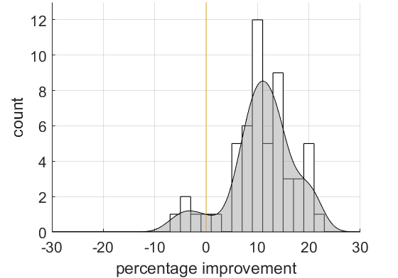
Figure 1: Percentage improvement of our method over Cheng et al. [12] for the median of the distance measures for an image set, where each image set is captured by a single model of a camera, and there are 11 image sets and 5 distance measures for each image set. For 50 (/55) times our method gave an improvement in the median. For 4 (/55) times, our method gave an increase in the median; the increases were all on one camera, the Canon 600D.

1.1 Contributions

Building on the work of Cheng et al. [12], in this paper we make the following contributions.

1. We show how multivariate regression trees [35, 13, 29], where each tree predicts multiple responses, can be used to effectively estimate an illuminant. In the case of multiple responses, multivariate trees are more compact than univariate trees and can be more accurate when the response variables are correlated [31]. In our method for illuminant estimation, each tree simultaneously predicts all three chromaticity components of an illuminant $\mathbf{e}=(r,g,b)$, rather than predicting them independently, thus taking into account that the chromaticity components of the illuminant are correlated and constrained.

2. We show how to fit a multivariate regression tree by directly minimizing a distance measure (loss function) of interest. Previous work on multivariate regression trees has addressed only variants of the well-known squared-error loss function [13, 30, 35]. However, for the distance or performance measures that have been proposed for white balancing, such as recovery angular error and reproduction angular error (see, e.g., [19, 22] and Section 2), the squared error is not the best surrogate for the distance measure of interest. We show how to efficiently fit multivariate trees for distance measures that have been proposed for white balancing.

3. We show empirically that overall our method leads to improved performance on diverse image sets. Our ensembles of multivariate regression trees are, with some exceptions, more accurate (see Figure 1 for a preliminary presentation of the improvement in accuracy) and are considerably simpler, while inheriting the fast run-time of Cheng et al.’s [12] approach.

2 Distance Measures

In this section, we review distance or performance measures that have been proposed for evaluating the effectiveness of white balancing algorithms. Although the distance measures are of course correlated, Finlayson and Zakizadeh [19] have shown that the ranking of white balancing algorithms will change depending on the chosen distance measure. The distance measures assume normalized RGB,

$$r=\frac{R}{R+G+B},~{}~{}~{}g=\frac{G}{R+G+B},~{}~{}~{}b=\frac{B}{R+G+B}$$

where $R$, $G$, and $B$ are the red, green, and blue channel measurements and $r+g+b=1$. In what follows, let all vectors be row vectors, $\hat{\mathbf{e}}=(\hat{r},\hat{g},\hat{b})$ be the estimated illuminant, and $\mathbf{e}=(r,g,b)$ be the ground truth illuminant.

The most widely used distance measure [22, 27], recovery angular error, measures the angular distance between the estimated illuminant and the ground truth illuminant,

$$\mathit{dist}_{\mathit{\theta}}(\bm{\hat{}}{\mathbf{e}},\mathbf{e})=\cos^{-1}\left(\frac{\bm{\hat{}}{\mathbf{e}}\cdot\mathbf{e}^{T}}{\|\bm{\hat{}}{\mathbf{e}}\|\|\mathbf{e}\|}\right),$$

where $\bm{\hat{}}{\mathbf{e}}\cdot\mathbf{e}^{T}$ is the dot product of the vectors, $\|\cdot\|$ is the Euclidean norm, and we assume the angular distance is measured in degrees. Gijsenij, Gevers, and Lucassen [22] note that human observers sometimes judge the recovery angular error to underestimate the perceived differences between two images. One reason is that the recovery angular error ignores the direction of the deviation from the ground truth, which can be important from a perceptual point of view.

Finlayson and Zakizadeh [19] propose reproduction angular error as a distance measure, where the angular error is determined after the image has been corrected with the estimated illuminant. Given an estimated illuminant $\bm{\hat{}}{\mathbf{e}}=(\bm{\hat{}}{r},\bm{\hat{}}{g},\bm{\hat{}}{b})$, a diagonal correction matrix is given by $D=\mathrm{diag}(\bm{\hat{}}{g}/\bm{\hat{}}{r},\bm{\hat{}}{g}/\bm{\hat{}}{g},\bm{\hat{}}{g}/\bm{\hat{}}{b})$. Once the correction has been applied to an image, the angular error between the white balanced ground truth and the target of uniform gray $\mathbf{1}=(1,1,1)$ can be determined,

$$\mathit{dist}_{\mathit{rep}}(\bm{\hat{}}{\mathbf{e}},\mathbf{e})= \cos^{-1}\left(\frac{(D\mathbf{e}^{T})^{T}\cdot\mathbf{1}^{T}}{\|D\mathbf{e}^{T}\|\|\mathbf{1}\|}\right)$$

$$= \cos^{-1}\left(\frac{r/\bm{\hat{}}{r}+g/\bm{\hat{}}{g}+b/\bm{\hat{}}{b}}{\sqrt{(r/\bm{\hat{}}{r})^{2}+(g/\bm{\hat{}}{g})^{2}+(b/\bm{\hat{}}{b})^{2}}\;\sqrt{3\vphantom{\bm{\hat{}}{b}^{2}}}}\right).$$

In other words, given a part of the image that is known to be achromatic, we are measuring how close in degrees it is to being achromatic once the image has been white balanced using the estimated illuminant.

Gijsenij et al. [22] discuss the use of the Minkowski distance for measuring the distance between the estimated and the ground truth illuminant. Two special cases are the Taxicab distance,

$$\mathit{dist}_{1}(\bm{\hat{}}{\mathbf{e}},\mathbf{e})=|\bm{\hat{}}{r}-r|+|\bm{\hat{}}{g}-g|+|\bm{\hat{}}{b}-b|,$$

and the Euclidean distance,

$$\mathit{dist}_{2}(\bm{\hat{}}{\mathbf{e}},\mathbf{e})=\sqrt{(\bm{\hat{}}{r}-r)^{2}+(\bm{\hat{}}{g}-g)^{2}+(\bm{\hat{}}{b}-b)^{2}}.$$

Gijsenij et al. [22] note that the Euclidean distance treats each of the RGB channels uniformly whereas it is known that the sensitivity of the human eye to perceived differences varies across color channels. To this end, Gijsenij et al. [22] define the perceptual Euclidean error,

$$\mathit{dist}_{\mathit{ped}}(\bm{\hat{}}{\mathbf{e}},\mathbf{e})=\sqrt{w_{r}(\bm{\hat{}}{r}-r)^{2}+w_{g}(\bm{\hat{}}{g}-g)^{2}+w_{b}(\bm{\hat{}}{b}-b)^{2}},$$

where weights $w_{r}$, $w_{g}$, and $w_{b}$ capture this sensitivity and $w_{r}+w_{g}+w_{b}=1$. In experiments, Gijsenij et al. [22] found that the weight vector $(w_{r},w_{g},w_{b})=(0.21,0.71,0.08)$ gave a higher correlation with the judgment of human observers than that of $\mathit{dist}_{\mathit{\theta}}$, $\mathit{dist}_{1}$, and $\mathit{dist}_{2}$.

3 Our Proposal

In this section, we present our approach for white balancing based on ensembles of multivariate regression trees. We begin with a brief review of univariate (ordinary) regression trees and how they were applied by Cheng et al. [12] for white balancing.

3.1 Univariate regression trees

Univariate regression trees are constructed in a greedy, top-down manner from a set of labeled training examples $\{(\mathbf{x}_{1},y_{1}),\ldots,(\mathbf{x}_{n},y_{n})\}$, where $\mathbf{x}_{i}=(x_{i1},\ldots,x_{im})$ is a vector of feature values and $y_{i}$ is a scalar response variable (see, e.g., [8, 33, 25]). As it is sufficient for our purposes, we assume that the feature values and the response variable are real-valued. The root node of the tree is associated with all the training examples. At each step in the construction of the tree, the training examples at a node are partitioned by choosing the feature $j\in\{1,\ldots,m\}$ and partition $p$ that minimizes the total of the squared-error loss functions,

$$\operatorname*{argmin}_{c_{1}}{\sum}_{i\in L(j,p)}(y_{i}-c_{1})^{2}~{}+~{}\operatorname*{argmin}_{c_{2}}{\sum}_{i\in R(j,p)}(y_{i}-c_{2})^{2},$$ (1)

where the partition is into two subsets, $L(j,p)$ and $R(j,p)$, formed by branching on feature $j$ according to $x_{ij}\leq p$ and $x_{ij}>p$, respectively. For the squared-error loss function, for any choice of feature $j$ and partition $p$ the minimization is solved by taking the scalar $c_{1}$ to be the mean of the $y_{i}$ values in the left branch and the scalar $c_{2}$ to be the mean of the $y_{i}$ values in the right branch (see, e.g., [25]). Once the best pair ($j,p)$ is found, a left child node and right child node are added to the tree and are associated with the subsets $L(j,p)$ and $R(j,p)$. The partitioning continues until some stopping criterion is met, in which case the node is a leaf and is labeled with the scalar $c$ associated with the subset of examples at the node.

To estimate an illuminant $\mathbf{e}=(r,g,b)$, Cheng et al. [12] predict the $r$ chromaticity and the $g$ chromaticity independently using separate univariate trees fit with the squared-error loss function and from these two values the estimate of the $b$ chromaticity can be determined using $b=1-r-g$. Cheng et al. [12] use four pairs of simple features in their univariate trees: ($f_{r}^{1}$, $f_{g}^{1}$), the mean color chromaticity as provided by the gray-world algorithm; ($f_{r}^{2}$, $f_{g}^{2}$), the brightest color chromaticity, an adaptation of the white-patch algorithm; ($f_{r}^{3}$, $f_{g}^{3}$), the bin average of the mode of the RGB histogram, and ($f_{r}^{4}$, $f_{g}^{4}$), the mode of the kernel density estimate from the normalized chromaticity plane. An important contribution of their work is a novel method for training and combining the predictions of an ensemble of trees using these features that is both fast and accurate, leading to the best overall performance to date on diverse image sets.

Two important points are that Cheng et al.’s [12] method (i) predicts the $r$ and $g$ chromaticities independently, and (ii) minimizes the distance measure of interest—in their work, the recovery angular error—indirectly by minimizing the squared-error loss function. Our starting point is (i) the observation that our response variable is not a scalar but a vector $\mathbf{e}=(r,g,b)$ of chromaticities, and (ii) the related observation that independently fitting using the squared-error loss function is not necessarily a good surrogate for minimizing distance measures used in white balancing (see Example 1).

Example 1.

Let $\mathbf{e}=(r,g,b)$ be the ground truth illuminant. Consider the two estimates of the illuminant $\bm{\hat{}}{\mathbf{e}}_{1}=(\bm{\hat{}}{r}_{1},\bm{\hat{}}{g}_{1},\bm{\hat{}}{b}_{1})$ and $\bm{\hat{}}{\mathbf{e}}_{2}=(\bm{\hat{}}{r}_{2},\bm{\hat{}}{g}_{2},\bm{\hat{}}{b}_{2})$, where

$$\bm{\hat{}}{r}_{1} =r+\alpha, \bm{\hat{}}{r}_{2} =r+\alpha,$$

$$\bm{\hat{}}{g}_{1} =g+\alpha, \bm{\hat{}}{g}_{2} =g-\alpha,$$

$$\bm{\hat{}}{b}_{1} =1-\bm{\hat{}}{r}_{1}-\bm{\hat{}}{g}_{1}=b-2\alpha, \bm{\hat{}}{b}_{2} =1-\bm{\hat{}}{r}_{2}-\bm{\hat{}}{g}_{2}=b,$$

and $\alpha>0$ is some residual error. Here, the pair of estimates $\bm{\hat{}}{r}_{1}$ and $\bm{\hat{}}{r}_{2}$ and the pair of estimates $\bm{\hat{}}{g}_{1}$ and $\bm{\hat{}}{g}_{2}$ both have equal squared error ($\alpha^{2}$). Thus, from the point of view of independently fitting using the squared-error loss function, the two estimates of the illuminant have equal error. However, for distance measures that have been proposed for white balancing (see Section 2), the error of the estimate $\bm{\hat{}}{\mathbf{e}}_{1}$ is larger (and can be much larger) than that of $\bm{\hat{}}{\mathbf{e}}_{2}$. For example, let $\mathbf{e}=(\frac{1}{3},\frac{1}{3},\frac{1}{3})$ and $\alpha=0.05$. For the recovery angular error, $\mathit{dist}_{\mathit{\theta}}(\bm{\hat{}}{\mathbf{e}}_{1},\mathbf{e})=11.977$ and $\mathit{dist}_{\mathit{\theta}}(\bm{\hat{}}{\mathbf{e}}_{2},\mathbf{e})=6.983$. Thus, minimizing the squared error is not necessarily a good surrogate for minimizing a distance measure of interest in white balancing.

Figure 2: An example multivariate regression tree when the distance measure is recovery angular error, showing only the first four layers (out of 18 layers). The three (green) leaf nodes are labeled with the number of training examples at that node and the illuminant estimation if that node is reached. Also shown are the four images associated with the bottom-most leaf node; the images have been gamma corrected for presentation.

3.2 Multivariate regression trees

Multivariate regression trees are constructed in a greedy, top-down manner from a set of labeled training examples $\{(\mathbf{x}_{1},\mathbf{y}_{1}),\ldots,(\mathbf{x}_{n},\mathbf{y}_{n})\}$, where as before $\mathbf{x}_{i}$ is a vector of feature values but now $\mathbf{y}_{i}=(y_{i1},\ldots,y_{ik})$ is a vector of response variables [35, 13, 29].

Our proposed method for illuminant estimation is for a single tree to simultaneously predict all three chromaticity components of an illuminant $\mathbf{e}=(r,g,b)$, rather than multiple trees predicting them independently, thus taking into account that the chromaticity components of the illuminant are correlated and constrained (see Figure 2). An innovation of our approach is to fit a multivariate regression tree by directly minimizing a distance measure (loss function) of interest. Previous work on multivariate regression trees has addressed only loss functions that are variants of the well-known squared-error loss function [13, 35]. In our proposed method, at each step in the construction of the multivariate regression tree, the training examples at a node are partitioned by choosing a feature $j\in\{1,\ldots,m\}$ and partition $p$ that minimizes the total of the loss functions,

$$\operatorname*{argmin}_{\bm{\hat{}}{\mathbf{e}}_{1}}{\sum}_{i\in L(j,p)}\mathit{dist}(\bm{\hat{}}{\mathbf{e}}_{1},\mathbf{e}_{i})~{}+~{}\operatorname*{argmin}_{\bm{\hat{}}{\mathbf{e}}_{2}}{\sum}_{i\in R(j,p)}\mathit{dist}(\bm{\hat{}}{\mathbf{e}}_{2},\mathbf{e}_{i}),$$ (2)

where the partition is into two subsets, $L(j,p)$ and $R(j,p)$, formed by branching on feature $j$ according to $x_{ij}\leq p$ and $x_{ij}>p$, respectively; $\mathit{dist}(\cdot,\cdot)$ is a distance measure that has been proposed for white balancing (see Section 2); and $\bm{\hat{}}{\mathbf{e}}_{1}$, $\bm{\hat{}}{\mathbf{e}}_{2}$, and $\mathbf{e}_{i}$ are normalized RGB vectors in $\mathbb{R}^{3}$, i.e., the chromaticities sum to one. The partitioning continues until some stopping criteria is met, in which case the node is a leaf and is labeled with the estimated illuminant $\bm{\hat{}}{\mathbf{e}}$ associated with the subset of examples at the node. When such a tree is used in white balancing an image that has not been seen before, one starts at the root and repeatedly tests the feature at a node and follows the appropriate branch until a leaf is reached. The label of the leaf is the estimated illuminant of the image.

3.3 Ensembles of multivariate regression trees

To improve predictive accuracy, an ensemble of trees is learned where each tree is a multivariate regression tree. Various methods have been proposed for constructing ensembles including manipulating the training examples, manipulating the input features, injecting randomness into the learning algorithm, and combinations of these methods (see [15]). We adopt the method for constructing ensembles that injects randomness into the construction of an individual tree. When constructing the tree, each feature $j$ partition $p$ pair considered in Equation 2 is accumulated along with the total of the loss functions associated with the pair. Rather than taking the $(j,p)$ pair that minimizes the total of the loss functions, a $(j,p)$ pair is chosen at random from all of the pairs that are within a given percentage of the minimum. This ensures that diverse yet accurate trees are constructed. We also experimented with bagging [6] and Cheng et al.’s method [12], two methods that manipulate the training examples to construct diverse trees, and with random forests [26, 7], a method that manipulates both the training examples and the input features. However, in each case the alternative led to a decrease in accuracy.

Given a new image, the individual predictions of the trees in the ensemble are combined into a single estimated illuminant $\bm{\hat{}}{\mathbf{e}}$ for the image as follows (see Figure 3). Let $S=\{\bm{\hat{}}{\mathbf{e}}_{1},\ldots,\bm{\hat{}}{\mathbf{e}}_{k}\}$ be the set of predictions from the individual trees. The final estimated illuminant is the normalized RGB vector $\bm{\hat{}}{\mathbf{e}}=(\bm{\hat{}}{r},\bm{\hat{}}{g},\bm{\hat{}}{b})$ that minimizes $\sum_{i\in S}\mathit{dist}(\bm{\hat{}}{\mathbf{e}},\bm{\hat{}}{\mathbf{e}}_{i})$; i.e., the same minimization problem as the one that is solved in partitioning the training examples at a node and in labeling a leaf when constructing the trees (Equation 2).

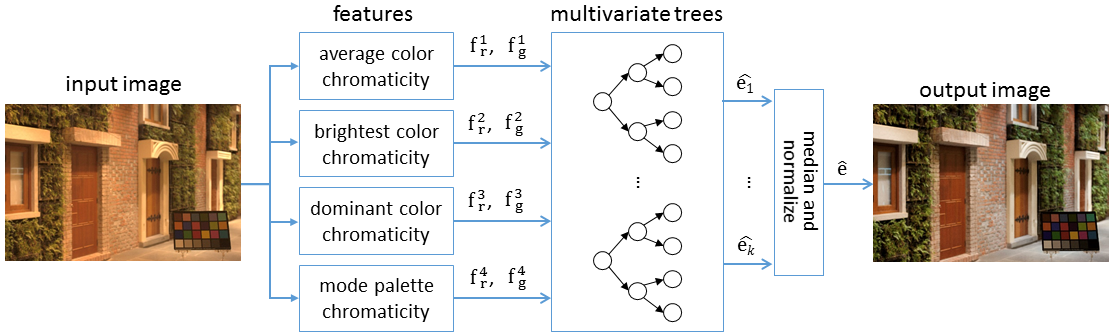
Figure 3: Our adaptation of Cheng et al.’s [12] learning-based method. Given an input image, four pairs of feature values are calculated, the feature values are used by each tree in the ensemble to predict the illumination, and the individual predictions $\{\bm{\hat{}}{\mathbf{e}}_{1},\ldots,\bm{\hat{}}{\mathbf{e}}_{k}\}$ are combined into a single estimate $\bm{\hat{}}{\mathbf{e}}$ of the illuminant that is used to white balance the image.

3.4 Fitting multivariate regression trees

In fitting a multivariate regression tree to a set of labeled training examples, the idea is to repeatedly, in a greedy and top-down manner, find the best feature $j$ and partition $p$ that results in the largest drop in the total error, as measured by a given distance measure (see Equation 2). The minimization in Equation 2 is a constrained, non-linear optimization problem. The problem must be solved many times when learning the ensemble of trees (approximately 40,000 calls to the minimization routine is typical for constructing a single tree) and also once every time the ensemble is applied to a new image and the individual predictions of the trees are combined to obtain a final estimated illuminant. Note that learning the trees is an offline process that occurs once while applying the ensemble to a new image is an online process that will occur many times, as it occurs each time an image is captured by the camera.

The minimization problem can be solved using exact but sophisticated and computationally expensive numerical optimization routines such as those based on interior-point or sequential quadratic programming methods. Exact methods are suitable for offline learning of a single ensemble of multivariate trees, but unfortunately are too slow for experimental evaluation where cross-validation and repeated trials are necessary to obtain accurate estimates of performance. This impediment also arises in univariate trees when using loss functions other than squared error (see, e.g., [25, p. 342]). As well, sophisticated exact methods are unlikely to be suitable for online application of the ensemble onboard the camera, given the real-time and space considerations.

Our proposed method is to solve the minimization problem approximately by taking the median of the ground truth illuminants of the training examples at a node and normalizing so that the RGB values sum to one (see Example 2). The method is simple and fast. As we show in supplementary material, the method often finds the exact solution and otherwise finds good quality approximate solutions for distance measures that arise in white balancing. Further, solving the minimization problem approximately does not appear to have a significant impact on the accuracy of the multivariate regression trees, perhaps because the tree construction itself is a greedy (and hence approximate) process.

Example 2.

Consider the follow three training examples, where the ground truth illuminants are shown but feature values are not shown, and let $\mathit{dist}_{2}$ be the distance measure.

example	r	g	b
$\mathbf{e}_{1}$	0.4285	0.4468	0.1247
$\mathbf{e}_{2}$	0.4221	0.4473	0.1306
$\mathbf{e}_{3}$	0.4098	0.4682	0.1220

Taking the median of the training examples gives (0.4221, 0.4473, 0.1247) and normalizing so that the RGB values sum to one results in the illuminant estimate (0.4246, 0.4500, 0.1254) with an associated cost of 3.5134. Taking the mean of the training examples results in the illuminant estimate (0.42012, 0.45411, 0.12577) with an associated cost of 3.7619. The illuminant estimate that exactly minimizes the sum of the distance measure over the training examples is (0.4228, 0.4487, 0.1285) with an associated cost of 3.4049.

4 Experimental Evaluation

In this section, we compare a MATLAB implementation of our multivariate regression tree method to Cheng et al.’s [12] method.

4.1 Image sets

We used the following image sets in our experiments.

SFU Laboratory image set. The SFU Laboratory image set consists of images of objects in a laboratory setting captured by a video camera under 11 different illuminants [2]. Following previous work, we use a common subset of 321 images (the minimal specularities and non-negligible dielectric specularities subset). A single image is the average of 50 video frames and is stored as a 16-bit TIFF file. In contrast to more recent image sets, the images are not captured as a camera RAW image file and thus have been processed by the camera. A white reference standard was used to determine ground truth, but the white reference does not appear in the images.

Gehler-Shi image set. The Gehler-Shi image set consists of 568 indoor and outdoor images captured by two different cameras [20, 36]. As done in previous work, we used the reprocessed version of the image set which starts from a camera RAW image file that has been minimally processed by the camera and creates a linearly processed, lossless 12-bit PNG file using the well-known dcraw program. Each image contains a color checker for determining ground truth.

NUS and NUS-Laboratory 8-camera image sets. The NUS 8-camera image set consists of 1736 images captured by eight different cameras [10], where in most cases each camera has photographed the same scene. Each image is captured as a minimally processed camera RAW image file and is linearly processed to create a lossless 16-bit PNG file. Each image contains a color checker for determining ground truth. The NUS-Laboratory 8-camera image set is a complementary laboratory set of 840 images captured with the same cameras. These additional images correct for a bias towards images captured outdoors in daylight [11].

Table 1: Comparison of accuracy of our proposed ensembles of multivariate regression trees against Cheng et al. [12] on the SFU Laboratory [2] image set, for various performance measures.

				tri-	best	worst
meas.	meth.	mean	med.	mean	25%	25%
Sony DXC-930, 321 images
$\mathit{dist}_{\mathit{\theta}}$	Cheng	4.24	2.24	2.85	0.35	11.29
	Ours	4.04	1.85	2.50	0.25	11.20
$\mathit{dist}_{\mathit{rep}}$	Cheng	4.62	2.68	3.24	0.43	11.95
	Ours	4.45	2.40	2.89	0.30	12.03
$\mathit{dist}_{\mathit{ped}}$	Cheng	2.07	1.18	1.45	0.19	5.35
	Ours	1.99	1.04	1.33	0.14	5.38

4.2 Experimental methodology

The main goal of our experiments is to compare our multivariate regression tree method—where each tree simultaneously predicts all three chromaticity components of an illuminant and the trees are fit by directly minimizing a distance measure of interest—to Cheng et al.’s [12] univariate tree method. To that end, we followed Cheng et al.’s [12] original experimental setup closely. In particular, we used the following methodology in our experimental evaluation.

Training data generation. Cheng et al. [12] use four pairs of simple features in their univariate trees (see the description in Section 3.1) and in our main set of experiments, we used the same features. In both approaches, training and testing is done on each camera separately; i.e., a predictive model is built for a particular model of camera rather than a generic model that can be used by any camera. To construct the machine learning data for a camera, each image taken by the camera in an image set is processed by (i) normalizing the image to a [0, 1] image, using the saturation level and darkness level of the camera, (ii) masking out the saturated pixels and the color checker, if present, (iii) determining the feature values for the image, and (iv) labeling the example using the ground truth illuminant. The result is a set of labeled training examples $\{(\mathbf{x}_{1},\mathbf{y}_{1}),\ldots,(\mathbf{x}_{n},\mathbf{y}_{n})\}$, where $\mathbf{x}_{i}=(f_{r}^{1},f_{g}^{1},\ldots,f_{r}^{4},f_{g}^{4})$ is a vector of feature values and $\mathbf{y}_{i}=(r_{i},g_{i},b_{i})$ is the ground truth illuminant.

Table 2: Comparison of accuracy of our proposed ensembles of multivariate regression trees against Cheng et al. [12] on the Gehler-Shi [36, 20] image set, for various distance measures.

				tri-	best	worst
meas.	meth.	mean	med.	mean	25%	25%
Canon 1D, 86 images
$\mathit{dist}_{\mathit{\theta}}$	Cheng	3.74	2.83	2.91	0.74	8.30
	Ours	3.57	2.45	2.75	0.81	8.13
$\mathit{dist}_{\mathit{rep}}$	Cheng	4.62	3.59	3.73	0.89	10.10
	Ours	4.38	3.21	3.53	0.92	9.66
$\mathit{dist}_{\mathit{ped}}$	Cheng	1.58	1.23	1.27	0.36	3.40
	Ours	1.53	1.10	1.20	0.37	3.41
Canon 5D, 482 images
$\mathit{dist}_{\mathit{\theta}}$	Cheng	2.18	1.37	1.54	0.35	5.42
	Ours	2.06	1.20	1.38	0.27	5.32
$\mathit{dist}_{\mathit{rep}}$	Cheng	2.85	1.77	2.00	0.42	7.13
	Ours	2.68	1.54	1.77	0.34	6.96
$\mathit{dist}_{\mathit{ped}}$	Cheng	0.96	0.63	0.70	0.17	2.30
	Ours	0.92	0.57	0.63	0.15	2.29

Parameter selection. In both approaches, parameters were set on 1/3 of the Gehler-Shi image set using $\mathit{dist}_{\mathit{\theta}}$ as the distance measure. The parameters were then fixed for all other cameras, image sets, and distance measures. Cheng et al. [12] set the following parameters: (i) the number of trees in an ensemble ($30\times 4\times 2=240$ trees, where each feature pair is used to build a tree for predicting $r$ and a tree for predicting $g$, and this is repeated 30 times), (ii) the amount of overlap and the number of slices of the training data used in constructing the ensemble, and (iii) a threshold value for determining the consensus of the ensemble. In our method, we set the following parameters: (i) the number of trees in an ensemble (30 trees), (ii) the amount of randomization used in constructing the ensemble (10%; see 3.3), and (iii) a threshold value, where a node is partitioned only if the average error at the node is greater than the threshold (0.5).

As well, Cheng et al. [12] use the MATLAB routine fitrtree for fitting a tree using the squared-error loss function. The routine has two parameters that were used at their default values: each branch node in the tree has at least “MinParentSize = 10” examples and each leaf has at least “MinLeafSize = 1” examples per tree leaf. These values are used as a stopping criteria when building the tree. We used the same stopping criteria in our implementation for fitting a tree using a chosen white balancing distance measure.

Table 3: Part I: Comparison of accuracy of our proposed ensembles of multivariate regression trees against Cheng et al. [12] on the combined NUS [10] and NUS-Laboratory 8-camera [11] image sets, for various distance measures.

				tri-	best	worst
meas.	meth.	mean	med.	mean	25%	25%
Canon EOS-1Ds Mark III, 364 images
$\mathit{dist}_{\mathit{\theta}}$	Cheng	2.13	1.45	1.61	0.36	5.06
	Ours	2.03	1.25	1.46	0.26	5.09
$\mathit{dist}_{\mathit{rep}}$	Cheng	2.81	1.89	2.14	0.46	6.71
	Ours	2.64	1.56	1.88	0.35	6.60
$\mathit{dist}_{\mathit{ped}}$	Cheng	1.00	0.70	0.76	0.19	2.32
	Ours	0.96	0.60	0.69	0.14	2.37
Canon EOS 600D, 305 images
$\mathit{dist}_{\mathit{\theta}}$	Cheng	2.21	1.55	1.67	0.45	5.12
	Ours	2.26	1.61	1.74	0.33	5.30
$\mathit{dist}_{\mathit{rep}}$	Cheng	2.92	2.04	2.23	0.57	6.76
	Ours	2.96	2.07	2.29	0.43	6.92
$\mathit{dist}_{\mathit{ped}}$	Cheng	1.01	0.72	0.78	0.23	2.32
	Ours	1.02	0.72	0.78	0.15	2.40
Fujifilm X-M1, 301 images
$\mathit{dist}_{\mathit{\theta}}$	Cheng	2.17	1.35	1.54	0.31	5.39
	Ours	2.19	1.21	1.46	0.23	5.72
$\mathit{dist}_{\mathit{rep}}$	Cheng	2.94	1.77	2.07	0.40	7.37
	Ours	3.00	1.60	1.99	0.32	7.94
$\mathit{dist}_{\mathit{ped}}$	Cheng	1.04	0.66	0.75	0.17	2.54
	Ours	1.04	0.59	0.72	0.12	2.72
Nikon D5200, 305 images
$\mathit{dist}_{\mathit{\theta}}$	Cheng	2.07	1.30	1.47	0.39	5.02
	Ours	2.03	1.15	1.34	0.30	5.18
$\mathit{dist}_{\mathit{rep}}$	Cheng	2.92	1.89	2.11	0.49	7.11
	Ours	2.87	1.64	1.95	0.40	7.36
$\mathit{dist}_{\mathit{ped}}$	Cheng	1.03	0.66	0.76	0.23	2.43
	Ours	0.99	0.59	0.69	0.16	2.46

Table 4: Part II: Comparison of accuracy of our proposed ensembles of multivariate regression trees against Cheng et al. [12] on the combined NUS [10] and NUS-Laboratory 8-camera [11] image sets, for various distance measures.

				tri-	best	worst
meas.	meth.	mean	med.	mean	25%	25%
Olympus E-PL6, 313 images
$\mathit{dist}_{\mathit{\theta}}$	Cheng	1.77	1.11	1.25	0.26	4.38
	Ours	1.77	1.02	1.18	0.23	4.56
$\mathit{dist}_{\mathit{rep}}$	Cheng	2.45	1.49	1.70	0.36	6.15
	Ours	2.46	1.39	1.60	0.32	6.41
$\mathit{dist}_{\mathit{ped}}$	Cheng	0.87	0.56	0.63	0.15	2.11
	Ours	0.86	0.50	0.58	0.13	2.20
Panasonic Lumix DMC-GX1, 308 images
$\mathit{dist}_{\mathit{\theta}}$	Cheng	2.22	1.41	1.57	0.36	5.47
	Ours	2.12	1.17	1.35	0.23	5.63
$\mathit{dist}_{\mathit{rep}}$	Cheng	3.02	1.92	2.17	0.45	7.44
	Ours	2.88	1.53	1.87	0.29	7.68
$\mathit{dist}_{\mathit{ped}}$	Cheng	1.03	0.68	0.75	0.21	2.44
	Ours	0.98	0.59	0.66	0.13	2.50
Samsung NX2000, 307 images
$\mathit{dist}_{\mathit{\theta}}$	Cheng	2.16	1.38	1.52	0.39	5.33
	Ours	2.15	1.30	1.47	0.33	5.45
$\mathit{dist}_{\mathit{rep}}$	Cheng	2.96	1.85	2.07	0.49	7.38
	Ours	2.94	1.71	1.97	0.42	7.55
$\mathit{dist}_{\mathit{ped}}$	Cheng	1.08	0.73	0.80	0.23	2.55
	Ours	1.08	0.71	0.77	0.19	2.62
Sony SLT-A57, 373 images
$\mathit{dist}_{\mathit{\theta}}$	Cheng	1.99	1.37	1.49	0.38	4.68
	Ours	1.86	1.09	1.29	0.28	4.65
$\mathit{dist}_{\mathit{rep}}$	Cheng	2.76	1.88	2.05	0.49	6.55
	Ours	2.54	1.49	1.78	0.38	6.37
$\mathit{dist}_{\mathit{ped}}$	Cheng	0.98	0.68	0.75	0.21	2.26
	Ours	0.94	0.55	0.66	0.16	2.34

Performance evaluation. We used standard $k$-fold cross validation, to evaluate and compare the accuracy of our method and Cheng et al.’s [12] method. In $k$-fold cross validation, the image set is randomly partitioned into $k$ approximately equal folds and each of the folds is, in turn, used as a testing set and the remaining $k-1$ folds are used as a training set. In our experiments we used 10-fold cross validation, as 10-fold is the most widely recommended, especially for our setting where the amount of data per camera is limited in some regions of the output space [28, 3, 25]. To reduce variance, the statistics we report are the result of performing 30 runs of 10-fold cross validation with different random seeds. Both methods share the same random seeds so that the partitions into training and test are the same for each algorithm for each experiment. Although for space considerations we only directly compare against Cheng et al.’s [12] method, we note that results comparing [12] to many other algorithms can be found in their original paper (the results reported here differ somewhat to those reported in [12] on common image sets as that paper uses 3-fold cross validation and reports results based on only a single run).

4.3 Experimental results

We compared the two approaches on accuracy, simplicity, and speed. All experiments were performed on a PC with an Intel i7-6700K, 4GHz running MATLAB R2016a.

Accuracy. Tables 1–4 show a comparison of the accuracy of our method of ensembles of multivariate regression trees against Cheng et al.’s [12] method on three distance measures (for space reasons results for distance measures $\mathit{dist}_{1}$ and $\mathit{dist}_{2}$ are omitted). For uniformity of presentation, the results for $\mathit{dist}_{\mathit{ped}}$ are multiplied by $10^{2}$. Note that, for each camera, in Cheng et al.’s [12] method an ensemble is fit once using the squared error and then evaluated on each of the distance measures, whereas in our method an ensemble is fit and evaluated on each of the distance measures. In practice, of course, in our method one would choose the distance measure that best fit with the intended purpose. It has been noted that the mean is a poor summary statistic in this context and more appropriate statistical measures are the median and the trimean [22, 27]. We also report the mean of the best 25% errors, and the mean of the worst 25% errors. Figure 1 summarizes the percentage improvement in accuracy for the median of all the distance measures. On these image sets, our method has improved accuracy for 10 out of 11 cameras and 50 out of 55 combinations of camera and distance measure. Only for one camera does our method lead to a decrease in accuracy and the percentage decrease in the median is bounded by 4.5%.

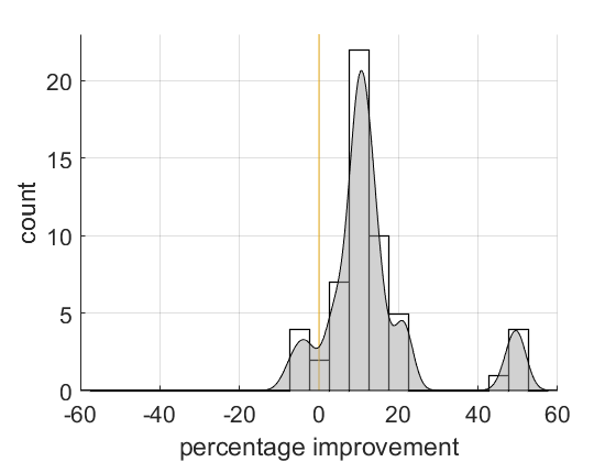
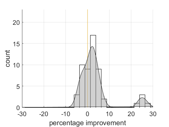
(a)	(b)

Figure 4: Percentage improvement of our method over Cheng et al. [12] when adding the feature shades-of-gray for (a) the median and (b) the mean of the worst 25% of the distance measures for an image set, where each image set is captured by a single model of a camera, and there are 11 image sets and 5 distance measures for each image set. For 50 (/55) times our method gave an improvement in the median and for 38 (/55) times our method gave an improvement in the mean of the worst 25%.

As can be seen in Figure 1 and Tables 1–4, our method compares favorably on the two statistics—median and trimean—that are arguably the most important in white balancing. Nevertheless, it can also be seen that Cheng et al.’s [12] method consistently outperforms our method on the mean of the worst 25% errors and it has been contended that reducing worst-case performance is also important [32]. In the experiments reported so far, we followed Cheng et al.’s [12] original experimental setup closely including using the same features. However, an examination of why our method did more poorly on the mean of the worst 25% errors suggested that our method was running out of predictive features when building our multivariate trees. We thus pursued a secondary set of experiments where we added one additional pair of features: ($f_{r}^{sg}$, $f_{g}^{sg}$), the color chromaticity as provided by the shades-of-gray algorithm [18]. The shades-of-gray algorithm is based on the $l_{p}$-norm, for $p=5$. Figure 4 summarizes the results and it can be seen that the addition of the feature improved the performance of our method on the worst cases, albeit at the expense of reducing the improvement on the median.

Simplicity. We also compared the size of the trees constructed by both methods. For the Canon 1Ds Mark III camera, we recorded the size of each tree and the size of each ensemble of trees, as measured by the number of nodes. The following table shows averages over 30 runs.

method	measure	tree	ensemble
Cheng	all	206.6	49,575.0
Ours	$\mathit{dist}_{\mathit{\theta}}$	143.9	4,317.2
	$\mathit{dist}_{\mathit{rep}}$	153.6	4,609.0
	$\mathit{dist}_{1}$	153.3	4,598.4
	$\mathit{dist}_{2}$	147.8	4,435.0
	$\mathit{dist}_{\mathit{ped}}$	110.9	3,327.6

It can be seen that our method leads to ensembles that are an order of magnitude smaller.

Speed. We also compared the speed of both methods. For the offline training of the trees, building our multivariate trees is considerably slower. For example, for the Canon EOS-1Ds Mark III camera and an image set of 364 images the times were 14.6 seconds versus 311.3 seconds. A partial reason is that Cheng et al. [12] use the MATLAB routine fitrtree for fitting a tree which automatically parallelizes training. For the online run-time, the two methods are for practical purposes identical, ours being negligibly faster due to having fewer trees in an ensemble, but both completing in approximately 0.5 seconds or less.

We conclude the experimental evaluation with a brief comparison to the current best-performing convolutional neural network (CNN) approach [37]. In terms of accuracy, on the NUS 8-camera image set, Shi et al. [37] report percentage improvements over Cheng et al. [12] of 5.1% for the mean, 8.2% for the median, and 3.4% for the trimean, where the improvement is measured over the geometric means of the eight cameras. As a point of comparison, on the combined NUS and NUS-Laboratory 8-camera image set, we achieve an improvement of 1.9% for the mean, 10.7% for the median, and 7.1% for the trimean, again as measured over the geometric means. In terms of simplicity and speed, the CNN approach is at a definite disadvantage. For example, Shi et al. [37] state that processing an image takes approximately 3 seconds on a GPU.

5 Conclusion

We show how multivariate regression trees, where each tree predicts multiple responses, can be used to effectively estimate an illuminant for white balancing an image. In our proposed method a multivariate regression tree is fit by directly minimizing a distance measure of interest. We show empirically that overall our method leads to improved performance on diverse image sets. Our ensembles of multivariate regression trees are, with some exceptions, more accurate and considerably simpler, while inheriting the fast run-time of previous work.

Appendix A Approximation error

Our proposed method is to solve approximately the minimization problem posed in Equation 2 for fitting multivariate trees (see Section 3.4). In this appendix, we report on experiments investigating the quality of the approximate solutions.

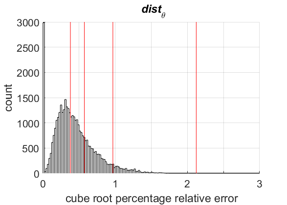
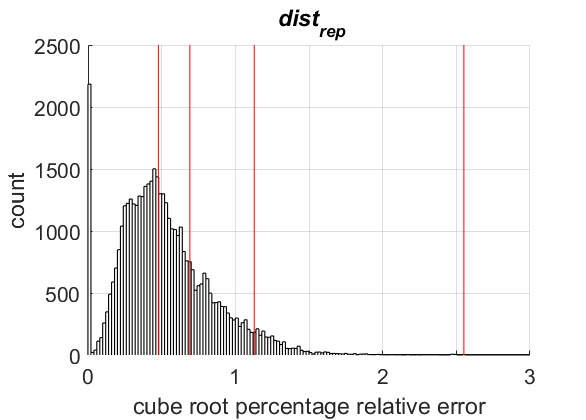
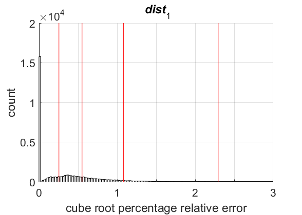
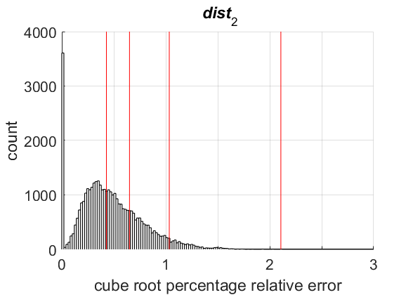
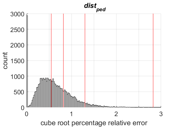
Figure 5: Percent relative approximation error on each call to the minimization routine when building one tree for the Canon EOS-1Ds Mark III camera. The red bars show the median, the 75th percentile, the 95th percentile, and the maximum. For visualization purposes, the results were transformed by taking the cube root of the percentage relative error.

For determining the exact solution to the minimization problems we used the MATLAB routine fmincon. Figure 5 shows how close to optimal the approximate solutions were for the various distance measures. The majority of the approximate solutions are within 1% of optimal.

References

- [1] N. Banić and S. Lonc̆arić. Color dog: Guiding the global illumination estimation to better accuracy. In Proceedings of the International Conference on Computer Vision Theory and Applications, 2015.
- [2] K. Barnard, L. Martin, A. Coath, and B. Funt. A comparison of computational color constancy algorithms II: Experiments with image data. IEEE Trans. on Image Processing, 11:985–996, 2002.
- [3] Y. Bengio and Y. Grandvalet. No unbiased estimator of the variance of k-fold cross-validation. Journal of Machine Learning Research, 5:1089–1105, 2004.
- [4] S. Bianco, G. Ciocca, C. Cusano, and R. Schettini. Automatic color constancy algorithm selection and combination. Pattern Recognition, 43:695–705, 2010.
- [5] S. Bianco, C. Cusano, and R. Schettini. Color constancy using CNNs. CoRR, abs/1504.04548, 2015.
- [6] L. Breiman. Bagging predictors. Machine Learning, 24:123–140, 1996.
- [7] L. Breiman. Random forests. Machine Learning, 45:5–32, 2001.
- [8] L. Breiman, J. Friedman, C. Stone, and R. Olshen. Classification and Regression Trees. CRC press, 1984.
- [9] V. C. Cardei, B. Funt, and K. Barnard. Estimating the scene illumination chromaticity by using a neural network. JOSA A, 19:2374–2386, 2002.
- [10] D. Cheng, D. K. Prasad, and M. S. Brown. Illuminant estimation for color constancy: Why spatial-domain methods work and the role of the color distribution. JOSA A, 31:1049–1058, 2014.
- [11] D. Cheng, B. Price, S. Cohen, and M. S. Brown. Beyond white: Ground truth colors for color constancy correction. In Proceedings of the IEEE International Conference on Computer Vision, pages 298–306, 2015.
- [12] D. Cheng, B. Price, S. Cohen, and M. S. Brown. Effective learning-based illuminant estimation using simple features. In Proceedings of the IEEE Conference on Computer Vision and Pattern Recognition, pages 1000–1008, 2015.
- [13] G. De’Ath. Multivariate regression trees: A new technique for modeling species-environment relationships. Ecology, 83(4):1105–1117, 2002.
- [14] Z. Deng, A. Gijsenij, and J. Zhang. Source camera identification using auto-white balance approximation. In Proceedings of the IEEE International Conference on Computer Vision, pages 57–64, 2011.
- [15] T. G. Dietterich. Ensemble methods in machine learning. In Proceedings of the International Workshop on Multiple Classifier Systems, pages 1–15, 2000. Available as: Springer Lecture Notes in Computer Science 1857.
- [16] G. D. Finlayson. Corrected-moment illuminant estimation. In Proceedings of the IEEE International Conference on Computer Vision, pages 1904–1911, 2013.
- [17] G. D. Finlayson, S. D. Hordley, and P. M. Hubel. Color by correlation: A simple, unifying framework for color constancy. IEEE Trans. on Pattern Analysis and Machine Intelligence, 23:1209–1221, 2001.
- [18] G. D. Finlayson and E. Trezzi. Shades of gray and colour constancy. In Proceedings of the Color and Imaging Conference, 2004.
- [19] G. D. Finlayson and R. Zakizadeh. Reproduction angular error: An improved performance metric for illuminant estimation. In Proceedings of the British Machine Vision Conference, 2014.
- [20] P. V. Gehler, C. Rother, A. Blake, T. Minka, and T. Sharp. Bayesian color constancy revisited. In Proceedings of the IEEE Conference on Computer Vision and Pattern Recognition, pages 1–8, 2008.
- [21] A. Gijsenij and T. Gevers. Color constancy using natural image statistics and scene semantics. IEEE Trans. on Pattern Analysis and Machine Intelligence, 33:687–698, 2011.
- [22] A. Gijsenij, T. Gevers, and M. P. Lucassen. Perceptual analysis of distance measures for color constancy algorithms. JOSA A, 26:2243–2256, 2009.
- [23] A. Gijsenij, T. Gevers, and J. van de Weijer. Generalized gamut mapping using image derivative structures for color constancy. IJCV, 86:127–139, 2010.
- [24] A. Gijsenij, T. Gevers, and J. van de Weijer. Computational color constancy: Survey and experiments. IEEE Trans. on Image Processing, 20:2475–2489, 2011.
- [25] T. Hastie, R. Tibshirani, and J. Friedman. The Elements of Statistical Learning: Data mining, Inference and Prediction. Springer, 2nd edition, 2009.
- [26] T. K. Ho. Random decision forests. In Proceedings of the 3rd International Conference on Document Analysis and Recognition, pages 278–282, 1995.
- [27] S. D. Hordley and G. D. Finlayson. Reevaluation of color constancy algorithm performance. JOSA A, pages 1008–1020, 2006.
- [28] R. Kohavi. A study of cross-validation and bootstrap for accuracy estimation and model selection. In Proceedings of the International Joint Conference on Artificial Intelligence, pages 1137–1145, 1995.
- [29] D. R. Larsen and P. L. Speckman. Multivariate regression trees for analysis of abundance data. Biometrics, 60(2):543–549, 2004.
- [30] W.-Y. Loh. Fifty years of classification and regression trees. International Statistical Review, 82(3):329–348, 2014.
- [31] W.-Y. Loh and W. Zheng. Regression trees for longtitudinal and multiresponse data. The Annals of Applied Statistics, 7(1):495–522, 2013.
- [32] M. Mosny and B. Funt. Reducing worst-case illumination estimates for better automatic white balance. In Proceedings of the Color and Imaging Conference, pages 52–56. Society for Imaging Science and Technology, 2012.
- [33] J. R. Quinlan. Induction of decision trees. Machine learning, 1(1):81–106, 1986.
- [34] C. Rosenberg, M. Hebert, and S. Thrun. Color constancy using KL-divergence. In Proceedings of the IEEE International Conference on Computer Vision, pages 239–246, 2001.
- [35] M. R. Segal. Tree structured methods for longitudinal data. J. American Statistical Association, 87:407–418, 1992.
- [36] L. Shi and B. Funt. Re-processed version of the Gehler color constancy dataset of 568 images. http://www.cs.sfu.ca/~colour/data.
- [37] W. Shi, C. C. Loy, and X. Tang. Deep specialized network for illuminant estimation. In Proceedings of the European Conference on Computer Vision, pages 371–387, 2016.
- [38] H. Vaezi Joze and M. Drew. Exemplar-based colour constancy and multiple illumination. IEEE Trans. on Pattern Analysis and Machine Intelligence, 36:860–873, 2014.
- [39] W. Xiong and B. Funt. Estimating illumination chromaticity via support vector regression. Journal of Imaging Science and Technology, 50(4):341–348, 2006.