Velocity-Density Correlations from the cosmicflows-3 Distance Catalog and the 2MASS Redshift Survey

Adi Nusser adi@physics.technion.ac.ilPhysics Department and the Asher Space Science Institute-Technion, Haifa 32000, Israel
Abstract

The peculiar velocity of a mass tracer is on average aligned with the dipole modulation of the surrounding mass density field. We present a first measurement of the correlation between radial peculiar velocities of objects in the cosmicflows-3 catalog and the dipole moment of the 2MRS galaxy distribution in concentric spherical shells centered on these objects. Limiting the analysis to cosmicflows-3 objects with distances of 100h1Mpc100superscript1Mpc100h^{-1}\,{\rm Mpc}, the correlation function is detected at a confidence level >4σsuperscriptsimilar-toabsent4𝜎\lower 2.15277pt\hbox{$\;\buildrel>\over{\sim}\;$}4\sigma. The measurement is found consistent with the standard ΛΛ\LambdaCDM model at <1.7σsuperscriptsimilar-toabsent1.7𝜎\lower 2.15277pt\hbox{$\;\buildrel<\over{\sim}\;$}1.7\sigma level. We formally derive the constraints 0.32<Ω0.55σ8<0.480.32superscriptΩ0.55subscript𝜎80.480.32<\Omega^{0.55}\sigma_{8}<0.48 (68%percent6868\% confidence level) or equivalently 0.34<Ω0.55/b<0.520.34superscriptΩ0.55𝑏0.520.34<\Omega^{0.55}/b<0.52, where b𝑏b is the galaxy bias factor. Deeper and improved peculiar velocity catalogs will substantially reduce the uncertainties, allowing tighter constraints from this type of correlations.

keywords:
dark matter – large-scale structure of Universe
pagerange: Velocity-Density Correlations from the cosmicflows-3 Distance Catalog and the 2MASS Redshift SurveyLABEL:lastpage

1 Introduction

The peculiar velocity of a galaxy is expected to be correlated with its surrounding matter distribution. A classic example is the motion of the Local Group (LG) of galaxies relative to the frame of reference defined by the temperature anisotropy of the cosmic microwave background (CMB). The dipole component of the CMB temperature implies a motion of Vlg=627±22kms1subscript𝑉l𝑔plus-or-minus62722kmsuperscripts1V_{\mathrm{l}g}=627\pm 22\ {\rm km\,s^{-1}} in the direction (l,b)=(276±3,30±3)𝑙𝑏plus-or-minussuperscript276superscript3plus-or-minussuperscript30superscript3(l,b)=(276^{\circ}\pm 3^{\circ},30^{\circ}\pm 3^{\circ}) (e.g. Kogut et al., 1993). In accordance with gravitational instability theory for structure formation (Peebles, 1980), this motion is produced by the cumulative gravitational pull of the observed large scale structure as probed by a variety of surveys of the galaxy distribution (e.g Strauss & Davis, 1988; Lynden-Bell et al., 1989; Schmoldt et al., 1999; Ciecielag & Chodorowski, 2004; Bilicki et al., 2011; Carrick et al., 2015). Any deviations can easily be explained within the limitations of current surveys (Nusser et al., 2014). More generally, the analysis of Davis et al. (2011) demonstrated a tight correlation between the observed radial velocities of galaxies in the SFI++ (Springob et al., 2007) catalog and the gravitational force field corresponding to the galaxy distribution in the Ks11.25subscript𝐾𝑠11.25K_{s}\leq 11.25 Two Mass Galaxy Redshift survey (2MRS) (Huchra et al., 2012).

The analyses above required a derivation of the gravitational field from a given distribution of galaxies in a redshift survey. In the case of the radial peculiar velocity versus gravity comparison, equivalent smoothing of the two fields is also essential. Here we aim at a simpler approach which can be implemented more directly, alleviating the complex steps in the analysis above. We aim at a direct measurement of the uδ𝑢𝛿u-\delta correlation between radial motion, u𝑢u, of galaxies and the dipole moment of the density contrast, δ𝛿\delta, on spherical shells centered on the galaxies. We will perform the correlation using the radial peculiar velocities from the cosmicflows-3 catalog (Tully et al., 2016) and the galaxy distribution in the Ks11.75subscript𝐾𝑠11.75K_{s}\leq 11.75 2MRS. These two data sets match in depth and are the best available in terms of sky coverage.

This uδ𝑢𝛿u-\delta correlation greatly mitigates several complications inherently present in the more detailed velocity-gravity comparison. As we shall see, by taking the dipole moment of the correlation function, the “Kaiser rocket” effect (Kaiser, 1988) resulting from the flux limit nature of the redshift survey is essentially eliminated. The estimation of the correlation does not require any smoothing of either the peculiar velocity data or the galaxy distribution.

The outline of the paper is as follows. In §2 we provide definitions for the basic quantities. The theoretical framework and predictions in the ΛΛ\LambdaCDM model are presented in §3. The main properties of the observational data, cosmicflows-3 and 2MRS, are briefly described in §4). This section also gives details of how the correlations are estimated from the observations. Errors associated with the observed correlations will be assessed using mock galaxy catalogs as described in §5. The results of uδ𝑢𝛿u-\delta correlations and implications on cosmological parameters follow in §6. In §6.3 we provide a preliminary assessment of 3D velocity density correlations. We conclude with a general discussion in §7.

Our notation is as follows. The expansion parameter is a𝑎a and is related to the redshift z𝑧z by a=(1+z)1𝑎superscript1𝑧1a=(1+z)^{-1}. The Hubble function is H(t)=a˙/a𝐻𝑡˙𝑎𝑎H(t)=\dot{a}/a and is denoted by H0subscript𝐻0H_{0} at the present epoch. We adopt the ΛΛ\LambdaCDM cosmological model denoting by ΩΩ\Omega and ΛΛ\Lambda the mass energy density parameters in units of the critical density. The growth factor of linear density perturbations is D(t)𝐷𝑡D(t) and the growth rate is f(z)=dlnD/dlna𝑓𝑧dln𝐷dln𝑎f(z)={\rm d}{\rm ln}D/{\rm d}{\rm ln}a. The growth rate mainly depends on the mass density parameter Ω(z)Ω𝑧\Omega(z) and is well approximated by fΩ0.55𝑓superscriptΩ0.55f\approx\Omega^{0.55} in a ΛΛ\LambdaCDM cosmology (Linder, 2005). Further, we define the correlation function ξfgf(rrr)g(rrr~)subscript𝜉𝑓𝑔delimited-⟨⟩𝑓rrr𝑔~rrr{\xi}_{{}_{fg}}\equiv\langle f(\kern-0.24994pt\hbox{$r$}\kern-4.78937pt\kern 0.50003pt\hbox{$r$}\kern-4.78937pt\kern-0.24994pt\raise 0.43304pt\hbox{$r$})g(\tilde{\kern-0.24994pt\hbox{$r$}\kern-4.78937pt\kern 0.50003pt\hbox{$r$}\kern-4.78937pt\kern-0.24994pt\raise 0.43304pt\hbox{$r$}})\rangle between any two fields f𝑓f and g𝑔g at points r𝑟rr𝑟rr𝑟r and rrr~~rrr\tilde{\kern-0.24994pt\hbox{$r$}\kern-4.78937pt\kern 0.50003pt\hbox{$r$}\kern-4.78937pt\kern-0.24994pt\raise 0.43304pt\hbox{$r$}} as the ensemble average over many random realizations of the fields.

2 Basics

The density contrast is defined as δ(rrr)=ρ(rrr)/ρ¯1𝛿rrr𝜌rrr¯𝜌1\delta(\kern-0.24994pt\hbox{$r$}\kern-4.78937pt\kern 0.50003pt\hbox{$r$}\kern-4.78937pt\kern-0.24994pt\raise 0.43304pt\hbox{$r$})=\rho(\kern-0.24994pt\hbox{$r$}\kern-4.78937pt\kern 0.50003pt\hbox{$r$}\kern-4.78937pt\kern-0.24994pt\raise 0.43304pt\hbox{$r$})/\bar{\rho}-1, where ρ¯¯𝜌\bar{\rho} is the mean background density. The comoving coordinate of a patch of matter is r𝑟rr𝑟rr𝑟r and the corresponding comoving peculiar velocity is v𝑣vv𝑣vv𝑣v (physical is avvv𝑎vvva\kern-0.24994pt\hbox{$v$}\kern-5.20601pt\kern 0.50003pt\hbox{$v$}\kern-5.20601pt\kern-0.24994pt\raise 0.43304pt\hbox{$v$}). Linear theory of cosmological gravitational instability (Peebles, 1980) relates v𝑣vv𝑣vv𝑣v and δ𝛿\delta via

δ(rrr)=1fvvv(rrr),𝛿rrr1𝑓vvvrrr\delta(\kern-0.24994pt\hbox{$r$}\kern-4.78937pt\kern 0.50003pt\hbox{$r$}\kern-4.78937pt\kern-0.24994pt\raise 0.43304pt\hbox{$r$})=-\frac{1}{f}\kern-0.24994pt\hbox{$\nabla$}\kern-8.33336pt\kern 0.50003pt\hbox{$\nabla$}\kern-8.33336pt\kern-0.24994pt\raise 0.43304pt\hbox{$\nabla$}\cdot\kern-0.24994pt\hbox{$v$}\kern-5.20601pt\kern 0.50003pt\hbox{$v$}\kern-5.20601pt\kern-0.24994pt\raise 0.43304pt\hbox{$v$}(\kern-0.24994pt\hbox{$r$}\kern-4.78937pt\kern 0.50003pt\hbox{$r$}\kern-4.78937pt\kern-0.24994pt\raise 0.43304pt\hbox{$r$})\;, (1)

where distance coordinates are expressed in kms1kmsuperscripts1\ {\rm km\,s^{-1}}. This, however, is the real density contrast corresponding to mass per unit volume d3r=r2drdΩsuperscriptd3𝑟superscript𝑟2d𝑟dΩ{\rm d}^{3}r=r^{2}{\rm d}r{\rm d}\Omega in actual distance space. Surveys of the galaxy distribution provide redshifts, cz𝑐𝑧cz (in kms1kmsuperscripts1\ {\rm km\,s^{-1}}), of galaxies rather than distances. The latter are provided in distance indicator catalogs for a smaller set of galaxies. The observed redshifts are given in terms of the comoving distance, r𝑟r, and the radial component u=vvvrrr^𝑢vvv^rrru=\kern-0.24994pt\hbox{$v$}\kern-5.20601pt\kern 0.50003pt\hbox{$v$}\kern-5.20601pt\kern-0.24994pt\raise 0.43304pt\hbox{$v$}\cdot\hat{\kern-0.24994pt\hbox{$r$}\kern-4.78937pt\kern 0.50003pt\hbox{$r$}\kern-4.78937pt\kern-0.24994pt\raise 0.43304pt\hbox{$r$}} of v𝑣vv𝑣vv𝑣v (Sachs & Wolfe, 1967),

cz=czc+u𝑐𝑧𝑐subscript𝑧𝑐𝑢cz=cz_{c}+u (2)

where zcsubscript𝑧𝑐z_{c} is the cosmological redshift calculated from the actual comoving distance111If rMpcsubscript𝑟Mpc{r}_{{}_{\mathrm{Mpc}}} is the comoving distance in Mpc then dr=HdrMpc=cdzc𝑑𝑟𝐻𝑑subscript𝑟Mpc𝑐𝑑subscript𝑧𝑐dr=Hd{r}_{{}_{\mathrm{Mpc}}}=cdz_{c} , r𝑟r, of the galaxy and, since we are considering low redshift data only, we have neglected gravitational contributions. By continuity and to linear order, density contrast of matter in redshift space, δssuperscript𝛿𝑠\delta^{s}, differs from δ𝛿\delta by the divergence of the displacement. Therefore,

δs=δ(urrr^).superscript𝛿𝑠𝛿𝑢^rrr\delta^{s}=\delta-\kern-0.24994pt\hbox{$\nabla$}\kern-8.33336pt\kern 0.50003pt\hbox{$\nabla$}\kern-8.33336pt\kern-0.24994pt\raise 0.43304pt\hbox{$\nabla$}\cdot(u\hat{\kern-0.24994pt\hbox{$r$}\kern-4.78937pt\kern 0.50003pt\hbox{$r$}\kern-4.78937pt\kern-0.24994pt\raise 0.43304pt\hbox{$r$}})\;. (3)

We write

(urrr^)=r^ir^jvixj+2ur,𝑢^rrrsubscript^𝑟𝑖subscript^𝑟𝑗subscript𝑣𝑖subscript𝑥𝑗2𝑢𝑟\kern-0.24994pt\hbox{$\nabla$}\kern-8.33336pt\kern 0.50003pt\hbox{$\nabla$}\kern-8.33336pt\kern-0.24994pt\raise 0.43304pt\hbox{$\nabla$}\cdot(u\hat{\kern-0.24994pt\hbox{$r$}\kern-4.78937pt\kern 0.50003pt\hbox{$r$}\kern-4.78937pt\kern-0.24994pt\raise 0.43304pt\hbox{$r$}})=\hat{r}_{i}\hat{r}_{j}\frac{\partial v_{i}}{\partial x_{j}}+\frac{2u}{r}\;, (4)

where r^isubscript^𝑟𝑖\hat{r}_{i} is cosine the angle between rrr^^rrr\hat{\kern-0.24994pt\hbox{$r$}\kern-4.78937pt\kern 0.50003pt\hbox{$r$}\kern-4.78937pt\kern-0.24994pt\raise 0.43304pt\hbox{$r$}} and the cartesian axis defined by the unit vector xxx^isubscript^xxx𝑖\hat{\kern-0.24994pt\hbox{$x$}\kern-5.71527pt\kern 0.50003pt\hbox{$x$}\kern-5.71527pt\kern-0.24994pt\raise 0.43304pt\hbox{$x$}}_{i} and summation over repeated indices is implied. The derivatives and all other quantities are taken as a function of the real space coordinate r𝑟r which, to linear order, are equivalent to quantities expressed in terms of coordinates in redshift space.

Therefore, observational data of radial peculiar motions and the distribution of galaxies in redshift space allow a direct estimation of the correlation function

ξuδs=u(rrr)δs(rrr~).superscriptsubscript𝜉𝑢𝛿𝑠delimited-⟨⟩𝑢rrrsuperscript𝛿𝑠~rrr{\xi}_{{}_{u\delta}}^{s}=\langle u(\kern-0.24994pt\hbox{$r$}\kern-4.78937pt\kern 0.50003pt\hbox{$r$}\kern-4.78937pt\kern-0.24994pt\raise 0.43304pt\hbox{$r$})\delta^{s}(\tilde{\kern-0.24994pt\hbox{$r$}\kern-4.78937pt\kern 0.50003pt\hbox{$r$}\kern-4.78937pt\kern-0.24994pt\raise 0.43304pt\hbox{$r$}})\rangle\;. (5)

rather than ξuδ=u(rrr)δ(rrr~)subscript𝜉𝑢𝛿delimited-⟨⟩𝑢rrr𝛿~rrr{\xi}_{{}_{u\delta}}=\langle u(\kern-0.24994pt\hbox{$r$}\kern-4.78937pt\kern 0.50003pt\hbox{$r$}\kern-4.78937pt\kern-0.24994pt\raise 0.43304pt\hbox{$r$})\delta(\tilde{\kern-0.24994pt\hbox{$r$}\kern-4.78937pt\kern 0.50003pt\hbox{$r$}\kern-4.78937pt\kern-0.24994pt\raise 0.43304pt\hbox{$r$}})\rangle between u𝑢u and the real space density field, δ𝛿\delta. The superscript s𝑠s on ξ𝜉\xi will be reserved for velocity-density correlation in redshift space.

The relation (3) implies

ξuδs=ξuδ+ξwu2ξuur~,superscriptsubscript𝜉𝑢𝛿𝑠subscript𝜉𝑢𝛿subscript𝜉𝑤𝑢2subscript𝜉𝑢𝑢~𝑟{\xi}_{{}_{u\delta}}^{s}=\xi_{u\delta}+{\xi}_{{}_{wu}}-\frac{2\xi_{uu}}{\tilde{r}}\;, (6)

where w=r~^ir~^jvi/x~j𝑤subscript^~𝑟𝑖subscript^~𝑟𝑗subscript𝑣𝑖subscript~𝑥𝑗w=-\hat{{\tilde{r}}}_{i}\hat{{\tilde{r}}}_{j}{\partial v_{i}}/{\partial\tilde{x}_{j}}. We begin with a theoretical description of ξuδssuperscriptsubscript𝜉𝑢𝛿𝑠{\xi}_{{}_{u\delta}}^{s} in linear theory and then we proceed to compute these correlations from mock and real data.

3 Theoretical correlations

Expressions for each of the terms on the r.h.s of (6) can be conveniently derived using the formalism developed by Gorski (1988) for describing velocity correlations. The correlation of the cartesian components visubscript𝑣𝑖v_{i} and vjsubscript𝑣𝑗v_{j} at different points in space is

ξvivj=Ψ(y)δijK+[Ψ(y)Ψ(y)]y^iy^j,subscript𝜉subscript𝑣𝑖subscript𝑣𝑗subscriptΨperpendicular-to𝑦subscriptsuperscript𝛿K𝑖𝑗delimited-[]subscriptΨparallel-to𝑦subscriptΨperpendicular-to𝑦subscript^𝑦𝑖subscript^𝑦𝑗{\xi}_{{}_{v_{i}v_{j}}}=\Psi_{\perp}(y)\delta^{\mathrm{K}}_{ij}+\left[\Psi_{\parallel}(y)-\Psi_{\perp}(y)\right]\hat{y}_{i}\hat{y}_{j}\;, (7)

where δijKsubscriptsuperscript𝛿K𝑖𝑗\delta^{\mathrm{K}}_{ij} is Kronecker’s delta function. The “perpendicular” and “parallel” (to the separation yyy=rrr~rrryyy~rrrrrr\kern-0.24994pt\hbox{$y$}\kern-5.2616pt\kern 0.50003pt\hbox{$y$}\kern-5.2616pt\kern-0.24994pt\raise 0.43304pt\hbox{$y$}=\tilde{\kern-0.24994pt\hbox{$r$}\kern-4.78937pt\kern 0.50003pt\hbox{$r$}\kern-4.78937pt\kern-0.24994pt\raise 0.43304pt\hbox{$r$}}-\kern-0.24994pt\hbox{$r$}\kern-4.78937pt\kern 0.50003pt\hbox{$r$}\kern-4.78937pt\kern-0.24994pt\raise 0.43304pt\hbox{$r$}) correlation functions ΨsubscriptΨperpendicular-to\Psi_{\perp} and ΨsubscriptΨparallel-to\Psi_{\parallel} are given in terms of the density power spectrum, P(k)𝑃𝑘P(k), as

Ψ,(y)=f22π20P(k)K,(ky)dk,\Psi_{\perp,\parallel}(y)=\frac{f^{2}}{2\pi^{2}}\int_{0}^{\infty}P(k)K_{\perp,\parallel}(ky){\rm d}k\;, (8)

where K(x)=j1(x)/xsubscript𝐾perpendicular-to𝑥subscript𝑗1𝑥𝑥K_{\perp}(x)=j_{1}(x)/x and K(x)=j0(x)2j1(x)/xsubscript𝐾parallel-to𝑥subscript𝑗0𝑥2subscript𝑗1𝑥𝑥K_{\parallel}(x)=j_{0}(x)-2j_{1}(x)/x and jl(x)subscript𝑗𝑙𝑥j_{l}(x) are spherical Bessel functions of order l𝑙l.

For ξuu=r^ivi(rrr)r~^jvj(rrr~)subscript𝜉𝑢𝑢delimited-⟨⟩subscript^𝑟𝑖subscript𝑣𝑖rrrsubscript^~𝑟𝑗subscript𝑣𝑗~rrr{\xi}_{{}_{uu}}=\langle\hat{r}_{i}v_{i}(\kern-0.24994pt\hbox{$r$}\kern-4.78937pt\kern 0.50003pt\hbox{$r$}\kern-4.78937pt\kern-0.24994pt\raise 0.43304pt\hbox{$r$})\hat{{\tilde{r}}}_{j}v_{j}(\tilde{\kern-0.24994pt\hbox{$r$}\kern-4.78937pt\kern 0.50003pt\hbox{$r$}\kern-4.78937pt\kern-0.24994pt\raise 0.43304pt\hbox{$r$}})\rangle, the relation (7) yields

ξuu=νΨ+μμ~Ψ,subscript𝜉𝑢𝑢𝜈subscriptΨperpendicular-to𝜇~𝜇subscriptΨ{\xi}_{{}_{uu}}=\nu\Psi_{\perp}+\mu\tilde{\mu}\Psi_{-}\;, (9)

where Ψ=ΨΨsubscriptΨsubscriptΨparallel-tosubscriptΨperpendicular-to\Psi_{-}=\Psi_{\parallel}-\Psi_{\perp}, μ=rrr^yyy^𝜇^rrr^yyy\mu=\hat{\kern-0.24994pt\hbox{$r$}\kern-4.78937pt\kern 0.50003pt\hbox{$r$}\kern-4.78937pt\kern-0.24994pt\raise 0.43304pt\hbox{$r$}}\cdot\hat{\kern-0.24994pt\hbox{$y$}\kern-5.2616pt\kern 0.50003pt\hbox{$y$}\kern-5.2616pt\kern-0.24994pt\raise 0.43304pt\hbox{$y$}}, μ~=rrr~^yyy^~𝜇^~rrr^yyy\tilde{\mu}=\hat{\tilde{\kern-0.24994pt\hbox{$r$}\kern-4.78937pt\kern 0.50003pt\hbox{$r$}\kern-4.78937pt\kern-0.24994pt\raise 0.43304pt\hbox{$r$}}}\cdot\hat{\kern-0.24994pt\hbox{$y$}\kern-5.2616pt\kern 0.50003pt\hbox{$y$}\kern-5.2616pt\kern-0.24994pt\raise 0.43304pt\hbox{$y$}} and ν=rrr^rrr~^𝜈^rrr^~rrr\nu=\hat{\kern-0.24994pt\hbox{$r$}\kern-4.78937pt\kern 0.50003pt\hbox{$r$}\kern-4.78937pt\kern-0.24994pt\raise 0.43304pt\hbox{$r$}}\cdot\hat{\tilde{\kern-0.24994pt\hbox{$r$}\kern-4.78937pt\kern 0.50003pt\hbox{$r$}\kern-4.78937pt\kern-0.24994pt\raise 0.43304pt\hbox{$r$}}}. To derive ξwusubscript𝜉𝑤𝑢{\xi}_{{}_{wu}}, we write 222y/x~i=y^i𝑦subscript~𝑥𝑖subscript^𝑦𝑖\partial y/\partial\tilde{x}_{i}=\hat{y}_{i} and y^i/x~j=δijK/y=y^iy^j/ysubscript^𝑦𝑖subscript~𝑥𝑗subscriptsuperscript𝛿K𝑖𝑗𝑦subscript^𝑦𝑖subscript^𝑦𝑗𝑦\partial\hat{y}_{i}/\partial\tilde{x}_{j}=\delta^{\mathrm{K}}_{ij}/y=\hat{y}_{i}\hat{y}_{j}/y where y=i(x~ixi)2𝑦subscript𝑖superscriptsubscript~𝑥𝑖subscript𝑥𝑖2y=\sqrt{\sum_{i}(\tilde{x}_{i}-x_{i})^{2}}.

vix~jvmdelimited-⟨⟩subscript𝑣𝑖subscript~𝑥𝑗subscript𝑣𝑚\displaystyle\langle\frac{\partial v_{i}}{\partial\tilde{x}_{j}}v_{m}\rangle =\displaystyle= Ψy^jδimK+Ψy^iy^jy^msubscriptsuperscriptΨperpendicular-tosubscript^𝑦𝑗subscriptsuperscript𝛿K𝑖𝑚subscriptsuperscriptΨsubscript^𝑦𝑖subscript^𝑦𝑗subscript^𝑦𝑚\displaystyle\Psi^{\prime}_{\perp}\hat{y}_{j}\delta^{\mathrm{K}}_{im}+\Psi^{\prime}_{-}\hat{y}_{i}\hat{y}_{j}\hat{y}_{m}
+\displaystyle+ Ψy(δijKy^m+δjmKy^i)2Ψyy^iy^jy^m.subscriptΨ𝑦subscriptsuperscript𝛿K𝑖𝑗subscript^𝑦𝑚subscriptsuperscript𝛿K𝑗𝑚subscript^𝑦𝑖2subscriptΨ𝑦subscript^𝑦𝑖subscript^𝑦𝑗subscript^𝑦𝑚\displaystyle\frac{\Psi_{-}}{y}\left(\delta^{\mathrm{K}}_{ij}\hat{y}_{m}+\delta^{\mathrm{K}}_{jm}\hat{y}_{i}\right)-2\frac{\Psi_{-}}{y}\hat{y}_{i}\hat{y}_{j}\hat{y}_{m}\;.

where primes denote derivatives with respect to y𝑦y. Therefore, contracting with r^ir^jsubscript^𝑟𝑖subscript^𝑟𝑗\hat{r}_{i}\hat{r}_{j} gives

ξwu=[Ψ(2μ~ν+μ)+(Ψ2Ψ)μ~2μ].subscript𝜉𝑤𝑢delimited-[]subscriptsuperscriptΨperpendicular-to2~𝜇𝜈𝜇subscriptsuperscriptΨ2subscriptsuperscriptΨperpendicular-tosuperscript~𝜇2𝜇{\xi}_{{}_{wu}}=-\left[\Psi^{\prime}_{\perp}(2\tilde{\mu}\;\nu+\mu)+(\Psi^{\prime}_{-}-2\Psi^{\prime}_{\perp}){\tilde{\mu}}^{2}\mu\right]\;. (11)

According to the linear relation (1), the correlation of u𝑢u with real space density is ξuδ=ξθu/fsubscript𝜉𝑢𝛿subscript𝜉𝜃𝑢𝑓{\xi}_{{}_{u\delta}}=-{\xi}_{{}_{\theta u}}/f where θ=vvv=δijKvix~j𝜃vvvsubscriptsuperscript𝛿K𝑖𝑗subscript𝑣𝑖subscript~𝑥𝑗\theta=\kern-0.24994pt\hbox{$\nabla$}\kern-8.33336pt\kern 0.50003pt\hbox{$\nabla$}\kern-8.33336pt\kern-0.24994pt\raise 0.43304pt\hbox{$\nabla$}\cdot\kern-0.24994pt\hbox{$v$}\kern-5.20601pt\kern 0.50003pt\hbox{$v$}\kern-5.20601pt\kern-0.24994pt\raise 0.43304pt\hbox{$v$}=\delta^{\mathrm{K}}_{ij}\frac{\partial v_{i}}{\partial\tilde{x}_{j}}. From (7) we have,

𝝃vvvθ=(3Ψ+Ψ)yyy^,subscript𝝃vvv𝜃3subscriptsuperscriptΨperpendicular-tosubscriptsuperscriptΨ^yyy{{\bm{\xi}}}_{{}_{\kern-0.12497pt\hbox{$v$}\kern-2.603pt\kern 0.25002pt\hbox{$v$}\kern-2.603pt\kern-0.12497pt\raise 0.21652pt\hbox{$v$}\theta}}=\left(3\Psi^{\prime}_{\perp}+\Psi^{\prime}_{-}\right)\hat{\kern-0.24994pt\hbox{$y$}\kern-5.2616pt\kern 0.50003pt\hbox{$y$}\kern-5.2616pt\kern-0.24994pt\raise 0.43304pt\hbox{$y$}}\;, (12)

where we have used Ψ=yΨsubscriptΨ𝑦subscriptsuperscriptΨperpendicular-to\Psi_{-}=y\Psi^{\prime}_{\perp} (Gorski, 1988). Thus, ξuθ=u(rrr)θ(rrr~)=rrr^𝝃vvvθsubscript𝜉𝑢𝜃delimited-⟨⟩𝑢rrr𝜃~rrr^rrrsubscript𝝃vvv𝜃{\xi}_{{}_{u\theta}}=\langle u(\kern-0.24994pt\hbox{$r$}\kern-4.78937pt\kern 0.50003pt\hbox{$r$}\kern-4.78937pt\kern-0.24994pt\raise 0.43304pt\hbox{$r$})\theta(\tilde{\kern-0.24994pt\hbox{$r$}\kern-4.78937pt\kern 0.50003pt\hbox{$r$}\kern-4.78937pt\kern-0.24994pt\raise 0.43304pt\hbox{$r$}})\rangle=\hat{\kern-0.24994pt\hbox{$r$}\kern-4.78937pt\kern 0.50003pt\hbox{$r$}\kern-4.78937pt\kern-0.24994pt\raise 0.43304pt\hbox{$r$}}\cdot{{\bm{\xi}}}_{{}_{\kern-0.12497pt\hbox{$v$}\kern-2.603pt\kern 0.25002pt\hbox{$v$}\kern-2.603pt\kern-0.12497pt\raise 0.21652pt\hbox{$v$}\theta}} and hence

ξuδ=1f(3Ψ+Ψ)μ.subscript𝜉𝑢𝛿1𝑓3subscriptsuperscriptΨperpendicular-tosubscriptsuperscriptΨ𝜇{\xi}_{{}_{u\delta}}=-\frac{1}{f}\left(3\Psi^{\prime}_{\perp}+\Psi^{\prime}_{-}\right)\mu\;. (13)

For later use we also list

ξuvj=r^ivi(rrr)vj(rrr~)=Ψr^j+μΨy^j.subscript𝜉𝑢subscript𝑣𝑗delimited-⟨⟩subscript^𝑟𝑖subscript𝑣𝑖rrrsubscript𝑣𝑗~rrrsubscriptΨperpendicular-tosubscript^𝑟𝑗𝜇subscriptΨsubscript^𝑦𝑗{\xi}_{{}_{uv_{j}}}=\langle\hat{r}_{i}v_{i}(\kern-0.24994pt\hbox{$r$}\kern-4.78937pt\kern 0.50003pt\hbox{$r$}\kern-4.78937pt\kern-0.24994pt\raise 0.43304pt\hbox{$r$})v_{j}(\tilde{\kern-0.24994pt\hbox{$r$}\kern-4.78937pt\kern 0.50003pt\hbox{$r$}\kern-4.78937pt\kern-0.24994pt\raise 0.43304pt\hbox{$r$}})\rangle=\Psi_{\perp}\hat{r}_{j}+\mu\Psi_{-}\hat{y}_{j}\;. (14)

Collecting all terms, we arrive at

ξuδs(rrr,rrr~)superscriptsubscript𝜉𝑢𝛿𝑠rrr~rrr\displaystyle{\xi}_{{}_{u\delta}}^{s}(\kern-0.24994pt\hbox{$r$}\kern-4.78937pt\kern 0.50003pt\hbox{$r$}\kern-4.78937pt\kern-0.24994pt\raise 0.43304pt\hbox{$r$},\tilde{\kern-0.24994pt\hbox{$r$}\kern-4.78937pt\kern 0.50003pt\hbox{$r$}\kern-4.78937pt\kern-0.24994pt\raise 0.43304pt\hbox{$r$}}) =\displaystyle= 1f(3Ψ+Ψ)μ1𝑓3subscriptsuperscriptΨperpendicular-tosubscriptsuperscriptΨ𝜇\displaystyle-\frac{1}{f}\left(3\Psi^{\prime}_{\perp}+\Psi^{\prime}_{-}\right)\mu
\displaystyle- 3ΨμΨ(2μ~ν+μ)(Ψ2Ψ)μ~2μ3subscriptsuperscriptΨperpendicular-to𝜇subscriptsuperscriptΨperpendicular-to2~𝜇𝜈𝜇subscriptsuperscriptΨ2subscriptsuperscriptΨperpendicular-tosuperscript~𝜇2𝜇\displaystyle 3\Psi^{\prime}_{\perp}\mu-\Psi^{\prime}_{\perp}(2\tilde{\mu}\;\nu+\mu)-(\Psi^{\prime}_{-}-2\Psi^{\prime}_{\perp}){\tilde{\mu}}^{2}\mu
\displaystyle- 2νΨ+μμ~Ψr~,2𝜈subscriptΨperpendicular-to𝜇~𝜇subscriptΨ~𝑟\displaystyle 2\frac{\nu\Psi_{\perp}+\mu\tilde{\mu}\Psi_{-}}{\tilde{r}}\;,

where ν𝜈\nu and μ~~𝜇\tilde{\mu} are expressed in terms of y𝑦y, r𝑟r and μ𝜇\mu.

The form of the dependence on μ𝜇\mu suggests a multipole expansion of the correlations by means of Legendre polynomials, Pl(μ)subscript𝑃𝑙𝜇P_{l}(\mu)333P0=1subscript𝑃01P_{0}=1, P1=μsubscript𝑃1𝜇P_{1}=\mu, P2=(3μ21)/2subscript𝑃23superscript𝜇212P_{2}=(3\mu^{2}-1)/2 and P3=(5μ33μ)/2subscript𝑃35superscript𝜇33𝜇2P_{3}=(5\mu^{3}-3\mu)/2. , Coefficients of the expansion can be computed easily in the separations y/r1much-less-than𝑦𝑟1y/r\ll 1, i.e. the distant observer limit (DOL), where ν1𝜈1\nu\approx 1 and μ~=μ~𝜇𝜇\tilde{\mu}=\mu. We will consider ξuδsl=1/(4π)dΩξuδsPl(μ)dμ=1/2dμξuδsPl(μ)subscriptdelimited-⟨⟩superscriptsubscript𝜉𝑢𝛿𝑠𝑙14𝜋differential-dΩsuperscriptsubscript𝜉𝑢𝛿𝑠subscript𝑃𝑙𝜇differential-d𝜇12differential-d𝜇superscriptsubscript𝜉𝑢𝛿𝑠subscript𝑃𝑙𝜇\langle{\xi}_{{}_{u\delta}}^{s}\rangle_{l}=1/(4\pi)\int{\rm d}\Omega{\xi}_{{}_{u\delta}}^{s}P_{l}(\mu){\rm d}\mu=1/2\int{\rm d}\mu{\xi}_{{}_{u\delta}}^{s}P_{l}(\mu). Evaluating the integrals gives

ξuδs0subscriptdelimited-⟨⟩superscriptsubscript𝜉𝑢𝛿𝑠0\displaystyle\langle{\xi}_{{}_{u\delta}}^{s}\rangle_{0} =\displaystyle= 2Ψ+2Ψ/3r~2subscriptΨperpendicular-to2subscriptΨ3~𝑟\displaystyle-\frac{2\Psi_{\perp}+2\Psi_{-}/3}{\tilde{r}} (16)
ξuδs1subscriptdelimited-⟨⟩superscriptsubscript𝜉𝑢𝛿𝑠1\displaystyle\langle{\xi}_{{}_{u\delta}}^{s}\rangle_{1} =\displaystyle= (35+1f)Ψ(1513f)Ψ351𝑓subscriptsuperscriptΨperpendicular-to1513𝑓subscriptsuperscriptΨ\displaystyle-\left(\frac{3}{5}+\frac{1}{f}\right)\Psi^{\prime}_{\perp}-\left(\frac{1}{5}-\frac{1}{3f}\right)\Psi^{\prime}_{-} (17)
ξuδs2subscriptdelimited-⟨⟩superscriptsubscript𝜉𝑢𝛿𝑠2\displaystyle\langle{\xi}_{{}_{u\delta}}^{s}\rangle_{2} =\displaystyle= 415Ψr~415subscriptΨ~𝑟\displaystyle-\frac{4}{15}\frac{\Psi_{-}}{\tilde{r}} (18)
ξuδs3subscriptdelimited-⟨⟩superscriptsubscript𝜉𝑢𝛿𝑠3\displaystyle\langle{\xi}_{{}_{u\delta}}^{s}\rangle_{3} =\displaystyle= 235(2ΨΨ),2352subscriptsuperscriptΨperpendicular-tosubscriptsuperscriptΨ\displaystyle\frac{2}{35}\left(2\Psi^{\prime}_{\perp}-\Psi^{\prime}_{-}\right)\;, (19)

and all higher moments vanish identically. The term 2ξuu/r~2subscript𝜉𝑢𝑢~𝑟2{\xi}_{{}_{uu}}/\tilde{r} contributes only to l=0𝑙0l=0 and l=2𝑙2l=2 and does not affect any of the other multipoles. Because of the 1/r1𝑟1/r dependence, this term mainly depends on nearby data.

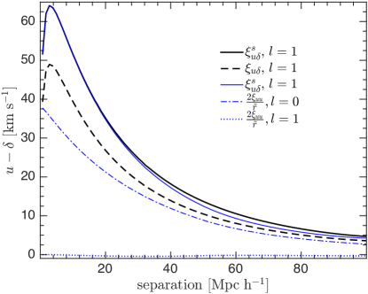
In figure 1 we plot a few of the relevant moments computed from the relations above for the ΛΛ\LambdaCDM cosmology with the Planck parameters. The multipoles l=2𝑙2l=2 and 333 are much smaller than the others and we opt not to show them. The l=0𝑙0l=0 moment of ξuu/r~subscript𝜉𝑢𝑢~𝑟{\xi}_{{}_{uu}}/\tilde{r} is substantial for r=50h1Mpc𝑟50superscript1Mpcr=50h^{-1}\,{\rm Mpc}. The multipole l=1𝑙1l=1 of this term vanishes identically only in the DOL. Nonetheless, it remains insignificant even away from this limit, as seen from the blue dotted curve at separations >r>𝑟~{}\hbox to0.0pt{$>$\hss}{\lower 4.30554pt\hbox{$\sim$}}r. Redshift space distortions boost the correlations with respect to real space due to large scale motions coherent with the density. This is reflected in the higher amplitude of ξuδsl=1subscriptdelimited-⟨⟩superscriptsubscript𝜉𝑢𝛿𝑠𝑙1\langle{\xi}_{{}_{u\delta}}^{s}\rangle_{l=1} (solid black for DOL and solid blue for r=50h1Mpc)r=50h^{-1}\,{\rm Mpc})) relative to the real space ξuδl=1subscriptdelimited-⟨⟩subscript𝜉𝑢𝛿𝑙1\langle{\xi}_{{}_{u\delta}}\rangle_{l=1} (dashed). As we shall see, the difference between the DOL and the r=50h1Mpc𝑟50superscript1Mpcr=50h^{-1}\,{\rm Mpc} results is insignificant compared to the errors associated with observations. The Kaiser rocket effect resulting from the flux limit nature of galaxy redshift surveys amounts to a term of the form ξuu/r~subscript𝜉𝑢𝑢~𝑟{\xi}_{{}_{uu}}/\tilde{r}, which is negligible in the l=1𝑙1l=1 moment of the correlation.

Refer to caption
Figure 1: Theoretical multipole moments of various terms in uδ𝑢𝛿u-\delta correlations, as indicated in the figure. The black solid and dashed curves are, respectively, the redshift and real space dipole (l=1𝑙1l=1) moment of the correlation in the distant observer limit with r=𝑟r=\infty. The blue lines are for the case where the u𝑢u is given at a distance r=50h1Mpc𝑟50superscript1Mpcr=50h^{-1}\,{\rm Mpc} from the origin.
Refer to caption
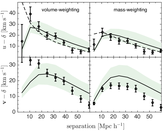
Figure 2: Top: Dipole moments, ζ𝜁\zeta, of the correlations ξuδssuperscriptsubscript𝜉𝑢𝛿𝑠{\xi}_{{}_{u\delta}}^{s} versus the separation, for the data (circles) and the mocks (solid and dashed in redshift and real space, respectively). The (1σ1𝜎1\sigma) error bars represent the scatter due random error in cosmicflows-3 velocities. Colored areas mark 1σ1𝜎1\sigma cosmic variance and shot noise in 2MRS, as given from the mocks. Panels to the left and to the right show ζVsuperscript𝜁𝑉\zeta^{V} and ζMsuperscript𝜁𝑀\zeta^{M}, respectively. Bottom: The same as Top but for 3D velocities reconstructed using Wiener filtering.

4 The observations

4.1 The distance indicator catalog

We use the grouped version of the cosmicflows-3 catalog (Tully et al., 2016) consisting of groups of galaxies as well as individual galaxies unassociated with groups. The total number of objects in the catalog is 6560 with 6200similar-toabsent6200{\sim}6200 having redshifts cz<15000kms1superscriptsimilar-to𝑐𝑧15000kmsuperscripts1cz\lower 2.15277pt\hbox{$\;\buildrel<\over{\sim}\;$}15000\ {\rm km\,s^{-1}}. The catalog provides measurements of redshifts, cz𝑐𝑧cz, and distance moduli, DM=25+5log10(DL/Mpc)𝐷𝑀255subscript10subscript𝐷𝐿MpcDM=25+5\log_{10}(D_{L}/\mathrm{Mpc}) where DLsubscript𝐷𝐿D_{L} is the luminosity distance. To infer the radial peculiar velocities, u𝑢u, we follow Tully et al. (2016) who use a prescription (Nusser & Davis, 1995; Nusser & Davis, 2011; Watkins & Feldman, 2014) that avoids introducing spurious non-gaussian errors at large distances.

Uncertainties in the determination of u𝑢u increase linearly with distance where the error in groups is reduced by the square root of the number of galaxies they respectively contain. Galaxies at large distances are prone to suffer from systematic biases and therefore we choose to restrict our analysis to objects within a maximum redshift of 10000kms110000kmsuperscripts110000\ {\rm km\,s^{-1}}, leaving us with 4600similar-toabsent4600{\sim}4600 objects.

4.2 The redshift survey

The distribution of galaxies in the flux limited 2MRS catalog (Huchra et al., 2012) will be correlated with peculiar velocities in cosmicflows-3. The 2MRS covers most of the sky down to Galactic latitudes of b5𝑏superscript5b\leq 5^{\circ} (8superscript88^{\circ} in the direction of the Bulge) and contains 45000similar-toabsent45000{\sim}45000 galaxies with spectroscopic redshifts and with apparent magnitudes Ks11.75subscript𝐾𝑠11.75K_{s}\leq 11.75. In order to account for the missing galaxies due to the flux limit each galaxy is assigned a weight

w=1/Φ(r),𝑤1Φ𝑟w=1/\Phi(r)\;, (20)

where ϕ(r)italic-ϕ𝑟\phi(r) is the selection function obtained from the F/T𝐹𝑇F/T estimator (Turner, 1979; Davis & Huchra, 1982) taking into account evolution and k-correction (figure 1 in Branchini et al., 2012). The galaxy number density contrast in a small volume, ΔVΔ𝑉\Delta V, is then estimated by

δg=1n¯rrrβΔVwβ1,superscript𝛿g1¯𝑛subscriptsubscriptrrr𝛽Δ𝑉subscript𝑤𝛽1\delta^{\mathrm{g}}=\frac{1}{\bar{n}}\sum_{\kern-0.17496pt\hbox{$r$}\kern-3.35255pt\kern 0.35002pt\hbox{$r$}\kern-3.35255pt\kern-0.17496pt\raise 0.30313pt\hbox{$r$}_{\beta}\in\Delta V}w_{\beta}-1\;, (21)

where wβ=w(rβ)subscript𝑤𝛽𝑤subscript𝑟𝛽w_{\beta}=w(r_{\beta}) and the sum is over all galaxies in ΔVΔ𝑉\Delta V. Further,

n¯=34πR3rβ<Rwβ¯𝑛34𝜋superscript𝑅3subscriptsubscript𝑟𝛽𝑅subscript𝑤𝛽\bar{n}=\frac{3}{4\pi R^{3}}\sum_{r_{\beta}<R}w_{\beta} (22)

is a proxy to the mean number density of galaxies, computed from the distribution of galaxies out to a sufficiently large radius R𝑅R. We take R=120h1Mpc𝑅120superscript1MpcR=120h^{-1}\,{\rm Mpc}, but n¯¯𝑛\bar{n} is robust for 80h1Mpc<R<200h1Mpcsuperscriptsimilar-to80superscript1Mpc𝑅superscriptsimilar-to200superscript1Mpc80h^{-1}\,{\rm Mpc}\lower 2.15277pt\hbox{$\;\buildrel<\over{\sim}\;$}R\lower 2.15277pt\hbox{$\;\buildrel<\over{\sim}\;$}200h^{-1}\,{\rm Mpc}, changing by less than a few percents.

4.3 Estimating correlations from the observations

Following the discussion in §3, we consider the dipole (l=1𝑙1l=1) moment only. We bin the separation, y𝑦y, into Nbsubscript𝑁𝑏N_{b} shells with radii ybsubscript𝑦𝑏y_{b} (b=1Nb)b=1\cdots N_{b}) of identical widths ΔyΔ𝑦\Delta y. For each galaxy, α𝛼\alpha, at rrrαsubscriptrrr𝛼\kern-0.24994pt\hbox{$r$}\kern-4.78937pt\kern 0.50003pt\hbox{$r$}\kern-4.78937pt\kern-0.24994pt\raise 0.43304pt\hbox{$r$}_{\alpha} in the cosmicflows-3 catalog we compute

Qα=yαβybwβμαβsubscript𝑄𝛼subscriptsubscript𝑦𝛼𝛽subscript𝑦𝑏subscript𝑤𝛽subscript𝜇𝛼𝛽Q_{\alpha}=\sum_{y_{\alpha\beta}\approx y_{b}}w_{\beta}\mu_{\alpha\beta} (23)

where β𝛽\beta indicates 2MRS galaxies at rrrβsubscriptrrr𝛽\kern-0.24994pt\hbox{$r$}\kern-4.78937pt\kern 0.50003pt\hbox{$r$}\kern-4.78937pt\kern-0.24994pt\raise 0.43304pt\hbox{$r$}_{\beta}, yyyαβ=rrrβrrrαsubscriptyyy𝛼𝛽subscriptrrr𝛽subscriptrrr𝛼\kern-0.24994pt\hbox{$y$}\kern-5.2616pt\kern 0.50003pt\hbox{$y$}\kern-5.2616pt\kern-0.24994pt\raise 0.43304pt\hbox{$y$}_{\alpha\beta}=\kern-0.24994pt\hbox{$r$}\kern-4.78937pt\kern 0.50003pt\hbox{$r$}\kern-4.78937pt\kern-0.24994pt\raise 0.43304pt\hbox{$r$}_{\beta}-\kern-0.24994pt\hbox{$r$}\kern-4.78937pt\kern 0.50003pt\hbox{$r$}\kern-4.78937pt\kern-0.24994pt\raise 0.43304pt\hbox{$r$}_{\alpha} and μαβ=yyyαβrrrβsubscript𝜇𝛼𝛽subscriptyyy𝛼𝛽subscriptrrr𝛽\mu_{\alpha\beta}=\kern-0.24994pt\hbox{$y$}\kern-5.2616pt\kern 0.50003pt\hbox{$y$}\kern-5.2616pt\kern-0.24994pt\raise 0.43304pt\hbox{$y$}_{\alpha\beta}\cdot\kern-0.24994pt\hbox{$r$}\kern-4.78937pt\kern 0.50003pt\hbox{$r$}\kern-4.78937pt\kern-0.24994pt\raise 0.43304pt\hbox{$r$}_{\beta} is cosine the angle between yyyαβsubscriptyyy𝛼𝛽\kern-0.24994pt\hbox{$y$}\kern-5.2616pt\kern 0.50003pt\hbox{$y$}\kern-5.2616pt\kern-0.24994pt\raise 0.43304pt\hbox{$y$}_{\alpha\beta} and rrrβsubscriptrrr𝛽\kern-0.24994pt\hbox{$r$}\kern-4.78937pt\kern 0.50003pt\hbox{$r$}\kern-4.78937pt\kern-0.24994pt\raise 0.43304pt\hbox{$r$}_{\beta}. The approximate symbol in the expression above implies that the summation is over galaxies with |yαβyb|<Δysubscript𝑦𝛼𝛽subscript𝑦𝑏Δ𝑦|y_{\alpha\beta}-y_{b}|<\Delta y. We consider two quantities,

ζV(yb)=1NvαQαn¯Vbuαsuperscript𝜁𝑉subscript𝑦𝑏1superscript𝑁vsubscript𝛼subscript𝑄𝛼¯𝑛subscript𝑉𝑏subscript𝑢𝛼\zeta^{V}(y_{b})=\frac{1}{N^{\mathrm{v}}}\sum_{\alpha}\frac{Q_{\alpha}}{\bar{n}V_{b}}u_{\alpha} (24)

and

ζM(yb)=1NvαQαn¯Vb(1+δbg)uαsuperscript𝜁𝑀subscript𝑦𝑏1superscript𝑁vsubscript𝛼subscript𝑄𝛼¯𝑛subscript𝑉𝑏1subscriptsuperscript𝛿g𝑏subscript𝑢𝛼{\zeta^{M}}(y_{b})=\frac{1}{N^{\mathrm{v}}}\sum_{\alpha}\frac{Q_{\alpha}}{\bar{n}V_{b}(1+\delta^{\mathrm{g}}_{b})}u_{\alpha} (25)

where Nvsuperscript𝑁vN^{\mathrm{v}} is the number of objects in the velocity catalog, n¯Vb¯𝑛subscript𝑉𝑏\bar{n}V_{b} is the mean number of galaxies in the volume Vbsubscript𝑉𝑏V_{b} occupied by the corresponding shell, and δbsubscript𝛿𝑏\delta_{b} is the mean density contrast inside Vbsubscript𝑉𝑏V_{b}. Both of these quantities reflect the dipole moment of ξuδssuperscriptsubscript𝜉𝑢𝛿𝑠{\xi}_{{}_{u\delta}}^{s}, but they have different physical meanings. While ζVsuperscript𝜁𝑉\zeta^{V} correlates u(rrr)𝑢rrru(\kern-0.24994pt\hbox{$r$}\kern-4.78937pt\kern 0.50003pt\hbox{$r$}\kern-4.78937pt\kern-0.24994pt\raise 0.43304pt\hbox{$r$}) with the dipole moment of the density in spherical shell centered on r𝑟rr𝑟rr𝑟r, the function ζMsuperscript𝜁𝑀\zeta^{M} correlates u𝑢u with the mean μ𝜇\mu per unit mass in the shell, i.e. it gives the same weighting to shells of different densities, δbgsubscriptsuperscript𝛿g𝑏\delta^{\mathrm{g}}_{b}. The function ζVsuperscript𝜁𝑉\zeta^{V} matches the basic definition of the l=1𝑙1l=1 multipole of the uδ𝑢𝛿u-\delta correlation, while ζMsuperscript𝜁𝑀\zeta^{M} significantly deviates from it in the non-linear regime where |δb|1similar-tosubscript𝛿𝑏1|\delta_{b}|\sim 1. Nonetheless, ζMsuperscript𝜁𝑀\zeta^{M} should serve as important test for the robustness of the results.

Let us explore these correlations in more detail. In the continuous limit

Qα(y)subscript𝑄𝛼𝑦\displaystyle Q_{\alpha}(y) \displaystyle\rightarrow n¯Vb21+1[1+δg(rrrα+yyy)]μdμ¯𝑛subscript𝑉𝑏2superscriptsubscript11delimited-[]1superscript𝛿gsubscriptrrr𝛼yyy𝜇differential-d𝜇\displaystyle\frac{\bar{n}V_{b}}{2}\int_{-1}^{+1}\left[1+\delta^{\mathrm{g}}(\kern-0.24994pt\hbox{$r$}\kern-4.78937pt\kern 0.50003pt\hbox{$r$}\kern-4.78937pt\kern-0.24994pt\raise 0.43304pt\hbox{$r$}_{\alpha}+\kern-0.24994pt\hbox{$y$}\kern-5.2616pt\kern 0.50003pt\hbox{$y$}\kern-5.2616pt\kern-0.24994pt\raise 0.43304pt\hbox{$y$})\right]\mu{\rm d}\mu
=\displaystyle= n¯Vb21+1δg(rrrα+yyy)μdμ¯𝑛subscript𝑉𝑏2superscriptsubscript11superscript𝛿gsubscriptrrr𝛼yyy𝜇differential-d𝜇\displaystyle\frac{\bar{n}V_{b}}{2}\int_{-1}^{+1}\delta^{\mathrm{g}}(\kern-0.24994pt\hbox{$r$}\kern-4.78937pt\kern 0.50003pt\hbox{$r$}\kern-4.78937pt\kern-0.24994pt\raise 0.43304pt\hbox{$r$}_{\alpha}+\kern-0.24994pt\hbox{$y$}\kern-5.2616pt\kern 0.50003pt\hbox{$y$}\kern-5.2616pt\kern-0.24994pt\raise 0.43304pt\hbox{$y$})\mu{\rm d}\mu

where now μ=rrr^αyyy^𝜇subscript^rrr𝛼^yyy\mu=\hat{\kern-0.24994pt\hbox{$r$}\kern-4.78937pt\kern 0.50003pt\hbox{$r$}\kern-4.78937pt\kern-0.24994pt\raise 0.43304pt\hbox{$r$}}_{\alpha}\cdot\hat{\kern-0.24994pt\hbox{$y$}\kern-5.2616pt\kern 0.50003pt\hbox{$y$}\kern-5.2616pt\kern-0.24994pt\raise 0.43304pt\hbox{$y$}} and δg(rrrα+yyy)superscript𝛿gsubscriptrrr𝛼yyy\delta^{\mathrm{g}}(\kern-0.24994pt\hbox{$r$}\kern-4.78937pt\kern 0.50003pt\hbox{$r$}\kern-4.78937pt\kern-0.24994pt\raise 0.43304pt\hbox{$r$}_{\alpha}+\kern-0.24994pt\hbox{$y$}\kern-5.2616pt\kern 0.50003pt\hbox{$y$}\kern-5.2616pt\kern-0.24994pt\raise 0.43304pt\hbox{$y$}) is the density contrast of the 2MRS galaxy distribution at the point rrrα+yyysubscriptrrr𝛼yyy\kern-0.24994pt\hbox{$r$}\kern-4.78937pt\kern 0.50003pt\hbox{$r$}\kern-4.78937pt\kern-0.24994pt\raise 0.43304pt\hbox{$r$}_{\alpha}+\kern-0.24994pt\hbox{$y$}\kern-5.2616pt\kern 0.50003pt\hbox{$y$}\kern-5.2616pt\kern-0.24994pt\raise 0.43304pt\hbox{$y$} in the shell. Hence,

ζV(y)12NvVvd3rrrnv(rrr)u(rrr)1+1δg(rrr+yyy)μdμ,superscript𝜁𝑉𝑦12superscript𝑁vsubscriptsuperscript𝑉vsuperscriptd3rrrsuperscript𝑛vrrr𝑢rrrsuperscriptsubscript11superscript𝛿grrryyy𝜇differential-d𝜇\zeta^{V}(y)\rightarrow\frac{1}{2N^{\mathrm{v}}}\int_{V^{\mathrm{v}}}{\rm d}^{3}\kern-0.24994pt\hbox{$r$}\kern-4.78937pt\kern 0.50003pt\hbox{$r$}\kern-4.78937pt\kern-0.24994pt\raise 0.43304pt\hbox{$r$}n^{\mathrm{v}}(\kern-0.24994pt\hbox{$r$}\kern-4.78937pt\kern 0.50003pt\hbox{$r$}\kern-4.78937pt\kern-0.24994pt\raise 0.43304pt\hbox{$r$})u(\kern-0.24994pt\hbox{$r$}\kern-4.78937pt\kern 0.50003pt\hbox{$r$}\kern-4.78937pt\kern-0.24994pt\raise 0.43304pt\hbox{$r$})\int_{-1}^{+1}\delta^{\mathrm{g}}(\kern-0.24994pt\hbox{$r$}\kern-4.78937pt\kern 0.50003pt\hbox{$r$}\kern-4.78937pt\kern-0.24994pt\raise 0.43304pt\hbox{$r$}+\kern-0.24994pt\hbox{$y$}\kern-5.2616pt\kern 0.50003pt\hbox{$y$}\kern-5.2616pt\kern-0.24994pt\raise 0.43304pt\hbox{$y$})\mu{\rm d}\mu\;, (27)

where Vvsuperscript𝑉vV^{\mathrm{v}} is the total volume encompassing the peculiar velocity catalog and nv(rrr)superscript𝑛vrrrn^{\mathrm{v}}(\kern-0.24994pt\hbox{$r$}\kern-4.78937pt\kern 0.50003pt\hbox{$r$}\kern-4.78937pt\kern-0.24994pt\raise 0.43304pt\hbox{$r$}) is the local number density of objects in the catalog, expressed as

nv(rrr)=n¯v[1+δv(rrr)]Sv(rrr),superscript𝑛vrrrsuperscript¯𝑛vdelimited-[]1superscript𝛿vrrrsuperscript𝑆vrrrn^{\mathrm{v}}(\kern-0.24994pt\hbox{$r$}\kern-4.78937pt\kern 0.50003pt\hbox{$r$}\kern-4.78937pt\kern-0.24994pt\raise 0.43304pt\hbox{$r$})=\bar{n}^{\mathrm{v}}\left[1+\delta^{\mathrm{v}}(\kern-0.24994pt\hbox{$r$}\kern-4.78937pt\kern 0.50003pt\hbox{$r$}\kern-4.78937pt\kern-0.24994pt\raise 0.43304pt\hbox{$r$})\right]S^{\mathrm{v}}(\kern-0.24994pt\hbox{$r$}\kern-4.78937pt\kern 0.50003pt\hbox{$r$}\kern-4.78937pt\kern-0.24994pt\raise 0.43304pt\hbox{$r$})\;, (28)

where n¯vsuperscript¯𝑛v\bar{n}^{\mathrm{v}} is the underlying mean number density of objects and δvsuperscript𝛿v\delta^{\mathrm{v}} is the underlying density contrast. Clearly δvsuperscript𝛿v\delta^{\mathrm{v}} and δgsuperscript𝛿g\delta^{\mathrm{g}} are closely related since they represent the underlying distribution of galaxies, albeit of different populations. The function Sv(rrr)superscript𝑆vrrrS^{\mathrm{v}}(\kern-0.24994pt\hbox{$r$}\kern-4.78937pt\kern 0.50003pt\hbox{$r$}\kern-4.78937pt\kern-0.24994pt\raise 0.43304pt\hbox{$r$}) represents various observational selections imposed on objects included in the velocity catalog. In contrast to flux limited redshift surveys, selection criteria on distance measurements are diverse and in general cannot be represented in a well defined form. However, it is reasonable to assume that none of these criteria depend on δvsuperscript𝛿v\delta^{\mathrm{v}}. Hence, Svsuperscript𝑆vS^{\mathrm{v}} is independent of δvsuperscript𝛿v\delta^{\mathrm{v}} and

Nv=n¯vd3rrrS(rrr).superscript𝑁vsuperscript¯𝑛vsuperscriptd3rrr𝑆rrrN^{\mathrm{v}}=\bar{n}^{\mathrm{v}}\int{\rm d}^{3}\kern-0.24994pt\hbox{$r$}\kern-4.78937pt\kern 0.50003pt\hbox{$r$}\kern-4.78937pt\kern-0.24994pt\raise 0.43304pt\hbox{$r$}S(\kern-0.24994pt\hbox{$r$}\kern-4.78937pt\kern 0.50003pt\hbox{$r$}\kern-4.78937pt\kern-0.24994pt\raise 0.43304pt\hbox{$r$})\;. (29)

Taking the ensemble average of the expression (27) we obtain

ζVsuperscript𝜁𝑉\displaystyle\zeta^{V} \displaystyle\rightarrow n¯vNvd3rrrS(rrr)ζ(r,y)superscript¯𝑛vsuperscript𝑁vsuperscriptd3rrr𝑆rrr𝜁𝑟𝑦\displaystyle\frac{\bar{n}^{\mathrm{v}}}{N^{\mathrm{v}}}\int{\rm d}^{3}\kern-0.24994pt\hbox{$r$}\kern-4.78937pt\kern 0.50003pt\hbox{$r$}\kern-4.78937pt\kern-0.24994pt\raise 0.43304pt\hbox{$r$}S(\kern-0.24994pt\hbox{$r$}\kern-4.78937pt\kern 0.50003pt\hbox{$r$}\kern-4.78937pt\kern-0.24994pt\raise 0.43304pt\hbox{$r$})\zeta(r,y)
+\displaystyle+ n¯v2Nvd3rrrS(rrr)δv(rrr)δg(rrr+yyy)u(rrr)μdμ.superscript¯𝑛v2superscript𝑁vsuperscriptd3rrr𝑆rrrdelimited-⟨⟩superscript𝛿vrrrsuperscript𝛿grrryyy𝑢rrr𝜇differential-d𝜇\displaystyle\frac{\bar{n}^{\mathrm{v}}}{2N^{\mathrm{v}}}\int{\rm d}^{3}\kern-0.24994pt\hbox{$r$}\kern-4.78937pt\kern 0.50003pt\hbox{$r$}\kern-4.78937pt\kern-0.24994pt\raise 0.43304pt\hbox{$r$}S(\kern-0.24994pt\hbox{$r$}\kern-4.78937pt\kern 0.50003pt\hbox{$r$}\kern-4.78937pt\kern-0.24994pt\raise 0.43304pt\hbox{$r$})\langle\delta^{\mathrm{v}}(\kern-0.24994pt\hbox{$r$}\kern-4.78937pt\kern 0.50003pt\hbox{$r$}\kern-4.78937pt\kern-0.24994pt\raise 0.43304pt\hbox{$r$})\delta^{\mathrm{g}}(\kern-0.24994pt\hbox{$r$}\kern-4.78937pt\kern 0.50003pt\hbox{$r$}\kern-4.78937pt\kern-0.24994pt\raise 0.43304pt\hbox{$r$}+\kern-0.24994pt\hbox{$y$}\kern-5.2616pt\kern 0.50003pt\hbox{$y$}\kern-5.2616pt\kern-0.24994pt\raise 0.43304pt\hbox{$y$})u(\kern-0.24994pt\hbox{$r$}\kern-4.78937pt\kern 0.50003pt\hbox{$r$}\kern-4.78937pt\kern-0.24994pt\raise 0.43304pt\hbox{$r$})\rangle\mu{\rm d}\mu\;.

The second term reflects a high order correlation between the density and velocity fields. We do not focus on this term although it is included in the correlations computed from the mocks used for comparison with data. This term is small on large scales. In the first term

ζ(r,y)12ξuδs(rrr,yyy)μdμ.𝜁𝑟𝑦12superscriptsubscript𝜉𝑢𝛿𝑠rrryyy𝜇differential-d𝜇\zeta(r,y)\equiv\frac{1}{2}\int{\xi}_{{}_{u\delta}}^{s}(\kern-0.24994pt\hbox{$r$}\kern-4.78937pt\kern 0.50003pt\hbox{$r$}\kern-4.78937pt\kern-0.24994pt\raise 0.43304pt\hbox{$r$},\kern-0.24994pt\hbox{$y$}\kern-5.2616pt\kern 0.50003pt\hbox{$y$}\kern-5.2616pt\kern-0.24994pt\raise 0.43304pt\hbox{$y$})\mu{\rm d}\mu\;. (31)

Thus the first term is an average of the dipole moment of the underlying linear correlation. Since ζ𝜁\zeta is independent of the direction of r𝑟rr𝑟rr𝑟r, this term is expressed as

4πn¯vNvdrr2S¯(r)ζ(r,y),4𝜋superscript¯𝑛vsuperscript𝑁vdifferential-d𝑟superscript𝑟2¯𝑆𝑟𝜁𝑟𝑦\frac{4\pi\bar{n}^{\mathrm{v}}}{N^{\mathrm{v}}}\int{\rm d}rr^{2}\bar{S}(r)\zeta(r,y)\;, (32)

where S¯¯𝑆\bar{S} is the angular average of S(rrr)𝑆rrrS(\kern-0.24994pt\hbox{$r$}\kern-4.78937pt\kern 0.50003pt\hbox{$r$}\kern-4.78937pt\kern-0.24994pt\raise 0.43304pt\hbox{$r$}), which is simply proportional to the radial distribution of objects in the velocity catalog and it is easily modeled. Further, in the distant observer limit ζ(r,y)ζ(y)𝜁𝑟𝑦𝜁𝑦\zeta(r,y)\approx\zeta(y) and we have ζVζsuperscript𝜁𝑉𝜁\zeta^{V}\rightarrow\zeta. To linear order ζM=ζVsuperscript𝜁𝑀superscript𝜁𝑉\zeta^{M}=\zeta^{V} despite the different physical meanings they carry. On small scales where deviations from linear theory are seen, we expect a smaller amplitude for ζMsuperscript𝜁𝑀\zeta^{M} as a result of weighting by the density.

In principle we could assign each cosmicflows-3 galaxy in this sum a weight determined by the observational error444Observational errors include intrinsic scatter in the distance indicator as well as purely instrumental measurement errors, σvsuperscript𝜎v\sigma^{\mathrm{v}}, in uαsubscript𝑢𝛼u_{\alpha}. Since the errors increase linearly with redshift, this procedure will heavily weigh nearer objects. The mean redshift of the cosmicflows-3 objects (survey depth)

cz¯=czα<czmaxwαvczα/wαv¯𝑐𝑧subscript𝑐subscript𝑧𝛼𝑐subscript𝑧maxsubscriptsuperscript𝑤v𝛼𝑐subscript𝑧𝛼subscriptsuperscript𝑤v𝛼\overline{cz}={\sum_{cz_{\alpha}<cz_{\mathrm{max}}}w^{\mathrm{v}}_{\alpha}cz_{\alpha}}/{\sum w^{\mathrm{v}}_{\alpha}} (33)

is 1000kms1similar-toabsent1000kmsuperscripts1{\sim}1000\ {\rm km\,s^{-1}} and 5000kms15000kmsuperscripts15000\ {\rm km\,s^{-1}}, respectively, for wv=(σv)2superscript𝑤vsuperscriptsuperscript𝜎v2w^{\mathrm{v}}=(\sigma^{\mathrm{v}})^{-2} and wv=(σv)1superscript𝑤vsuperscriptsuperscript𝜎v1w^{\mathrm{v}}=(\sigma^{\mathrm{v}})^{-1}, both for unrestricted czmax𝑐subscript𝑧maxcz_{\mathrm{max}}. Results in this paper will be given with w=1𝑤1w=1 including objects with within czmax=10000kms1𝑐subscript𝑧max10000kmsuperscripts1cz_{\mathrm{max}}=10000\ {\rm km\,s^{-1}}, corresponding cz¯=8000kms1¯𝑐𝑧8000kmsuperscripts1\overline{cz}=8000\ {\rm km\,s^{-1}}. This equal weighting of all galaxies within czmax𝑐subscript𝑧maxcz_{\mathrm{max}} comes at the expense of increased statistical error on the estimated correlations. Fortunately, as we shall see, the main source of uncertainty in the determination of the correlation is cosmic variance rather than velocity observational errors. The reason for imposing the redshift cut, czmax𝑐subscript𝑧maxcz_{\mathrm{max}} is to avoid potential systematic errors in the data, which are more likely at larger distances.

We place objects (galaxies and groups) in the peculiar velocity catalog at their comoving distance positions, r(z)𝑟𝑧r(z), computed from observed redshifts, cz𝑐𝑧cz, rather than distances, resubscript𝑟er_{\mathrm{e}}, estimated from the distance indicator measurements. Although the inferred peculiar velocities, u𝑢u, are the same, the placement of objects at resubscript𝑟er_{\mathrm{e}} introduces severe spatial Malmquist biases associated with large random errors (Lynden-Bell et al., 1988; Strauss & Willick, 1995). Non-linear and incoherent motions on small scales spoil the one-to-one mapping between distance and redshift and play the role of random errors when objects are placed at their redshift coordinates. Thus Malmquist biases are present in redshift space as well. These small scale motions are 200kms1similar-toabsent200kmsuperscripts1{\sim}200\ {\rm km\,s^{-1}} while distance errors are (0.150.2)czsimilar-toabsent0.150.2𝑐𝑧{\sim}(0.15-0.2)cz. Thus, working in redshift space, especially at large distances greatly mitigates the effects of Malmquist biases limiting them to scales of a few Mpc anyways. We will be interested in the correlation signal on scales of 10s of Mpcs, implying that the effect of small scale motions is entirely negligible. Note that the 2MRS galaxy distribution is smeared out along the line of sight due to these motions. This prevents the recovery of the underlying signal on a few Mpc scale even with perfect peculiar velocity data.

A peculiarity of our local cosmological neighborhood is the remarkable coherence of the flow of galaxies within a few Mpcs around us (e.g. Tully et al., 2013). With respect to the CMB frame of reference, the bulk flow around us starts with 630kms1similar-toabsent630kmsuperscripts1{\sim}630\ {\rm km\,s^{-1}} for the LG and smoothly reaches 270kms1similar-toabsent270kmsuperscripts1{\sim}270\ {\rm km\,s^{-1}} in a sphere of radius 100h1Mpc100superscript1Mpc100h^{-1}\,{\rm Mpc} centered on the observer (Nusser & Davis, 2011). Thus, the distribution of galaxies defined by redshifts with respect to the CMB exhibits a large spurious local inhomogeneity. To avoid this behavior we work with redshifts transformed to the LG frame of reference. However, a coherent galaxy distribution is not the only reason for choosing this frame of reference. The LG motion is generated by the cumulative gravitational of the large scale structure out to >300h1Mpcsuperscriptsimilar-toabsent300superscript1Mpc\lower 2.15277pt\hbox{$\;\buildrel>\over{\sim}\;$}300h^{-1}\,{\rm Mpc} (Bilicki et al., 2011; Nusser et al., 2014) and beyond. These distant (external) structures contribute also to the velocities of cosmicflows-3 objects with respect to the CMB, as indicated by the value of bulk flow within czmax/H0=100h1Mpc𝑐subscript𝑧max𝐻0100superscript1Mpccz_{\mathrm{max}}/H0=100h^{-1}\,{\rm Mpc}. The main contribution of external structures is to the dipole moments of the velocity field on shells around us. However, the dipole component of the velocity field relative to the LG motion is entirely determined by the mass distribution between the LG and the shell (Nusser & Davis, 1994). Therefore, working in the LG frame will exclude a velocity component which is uncorrelated with the density field surrounding an object in the cosmicflows-3 catalog.

5 Mock Catalogs

We use 30 mock catalogs of 2MRS extracted by Keselman & Nusser (2016) from the Dark-Sky public Simulations (Skillman et al., 2014) of the ΛΛ\LambdaCDM cosmology with Ω=0.295Ω0.295\Omega=0.295 , baryonic density parameter Ωb=0.0468subscriptΩ𝑏0.0468\Omega_{b}=0.0468, Λ=0.705Λ0.705\Lambda=0.705, h=0.6880.688h=0.688, and rms mass density fluctuations in spheres of 8h1Mpc8superscript1Mpc8h^{-1}\,{\rm Mpc} of σ8=0.835subscript𝜎80.835\sigma_{8}=0.835. The parameters are very close to the Planck values (e.g. column 4 of Table 3 in Planck Collaboration et al., 2016). These are dark matter only simulations, but baryonic feedback is too weak to play any significant role over the relevant level of accuracy and scales considered (Hellwing et al., 2016) The simulations are available with 5 different resolutions. The mocks are based on the simulation of 40963superscript409634096^{3} particles in a periodic box of 800h1Mpc800superscript1Mpc800h^{-1}\,{\rm Mpc} on the side, corresponding to a particle mass of 6.1×10⁸h1M6.1superscript108superscript1subscript𝑀direct-product6.1\times 10^{8}h^{-1}M_{\odot}. We consider halos containing no less than 50 particles, giving a minimal halo mass of 3.05×10¹⁰h1M3.05superscript1010superscript1subscript𝑀direct-product3.05\times 10^{10}h^{-1}M_{\odot}.

Mock “observers” are selected to reside in host halos of mass >5×10¹¹h1Msuperscriptsimilar-toabsent5superscript1011superscript1subscript𝑀direct-product\lower 2.15277pt\hbox{$\;\buildrel>\over{\sim}\;$}5\times 10^{11}h^{-1}M_{\odot} corresponding to a Milky Way halo mass with no neighboring rich clusters (>1015h1Msuperscriptsimilar-toabsentsuperscript1015superscript1subscript𝑀direct-product\lower 2.15277pt\hbox{$\;\buildrel>\over{\sim}\;$}10^{15}h^{-1}M_{\odot}) within a distance of 20 h1Mpcsuperscript1Mpch^{-1}\,{\rm Mpc}. Further, the bulk velocity within spheres of radii 3, 5, and 7 h1Mpcsuperscript1Mpch^{-1}\,{\rm Mpc} centered on the observers do not differ by more than 50kms150kmsuperscripts150\ {\rm km\,s^{-1}}.

Halos above a mass threshold Mhsubscript𝑀M_{h} are identified as mock galaxies. The mass threshold depends on the distance from the observer in each catalog in order to match the selection function of the 2MRS galaxies (Branchini et al., 2012). Each catalog is trimmed at a maximum distance of 200h1Mpc200superscript1Mpc200h^{-1}\,{\rm Mpc} and contains 42000similar-toabsent42000\sim 42000 galaxies similar to the real 2MRS.

Similarly to σ8subscript𝜎8\sigma_{8} for the underlying mass density field, we define σ8gsuperscriptsubscript𝜎8g\sigma_{8}^{\mathrm{g}} as the rms of the fluctuations in the galaxy number density contrast in spheres of 8h1Mpc8superscript1Mpc8h^{-1}\,{\rm Mpc} in radius. We also define b=σ8g/σ8𝑏superscriptsubscript𝜎8gsubscript𝜎8b=\sigma_{8}^{\mathrm{g}}/\sigma_{8} as the galaxy bias factor. Direct calculation of σ8gsuperscriptsubscript𝜎8g\sigma_{8}^{\mathrm{g}} in the mocks in real space yields bmock0.96superscript𝑏m𝑜𝑐𝑘0.96b^{\mathrm{m}ock}\approx 0.96, i.e. the mock galaxies are slightly anti-biased. We have directly calculated σ8gsuperscriptsubscript𝜎8g\sigma_{8}^{\mathrm{g}} in the 2MRS catalog from randomly placed spheres. The result depends slightly on the volume chosen to contain the spheres. We obtain 0.98<σ8g<1.070.98superscriptsubscript𝜎8g1.070.98<\sigma_{8}^{\mathrm{g}}<1.07 for spherical volumes of radii 80140h1Mpc80140superscript1Mpc80-140h^{-1}\,{\rm Mpc}. Thus, we adopt σ8g=1.02±0.05superscriptsubscript𝜎8gplus-or-minus1.020.05\sigma_{8}^{\mathrm{g}}=1.02\pm 0.05 (cf. Westover, 2007). We are interested in σ8gsuperscriptsubscript𝜎8g\sigma_{8}^{\mathrm{g}} computed from the galaxy distribution in real space. Assuming the ratio of σ8gsuperscriptsubscript𝜎8g\sigma_{8}^{\mathrm{g}} in redshift to real space is the same as in the mocks we derive σ8g=0.93±0.05superscriptsubscript𝜎8gplus-or-minus0.930.05\sigma_{8}^{\mathrm{g}}=0.93\pm 0.05 for 2MRS in real space Adopting the Planck σ8=0.831subscript𝜎80.831\sigma_{8}=0.831 (Planck Collaboration et al., 2016) for σ8subscript𝜎8\sigma_{8} of underlying mass, yields the 2MRS bias factor of b2MRS=1.12±0.06superscript𝑏2MRSplus-or-minus1.120.06b^{\mathrm{2MRS}}=1.12\pm 0.06.

Mock cosmicflows-3 galaxies are selected at random the 2MRS mocks with a distance dependent probability designed to produce a radial distribution of objects, consistent with the cosmicflows-3 catalog. The mean number of galaxies in the mocks within 100h1Mpc100superscript1Mpc100h^{-1}\,{\rm Mpc} is 4300, similar to the observations. We refrain from adding errors to the mock cosmicflows-3 objects since the observed errors vary depending on the type of distance indicator used and whether the object is a group or a individual galaxy. The effect of random errors on the correlations is done via a “bootstrap” procedure described in the next section.

6 Results

6.1 uδ𝑢𝛿u-\delta correlations

The top panels in figure 2 show the correlations ζ𝜁\zeta computed from the data and the mocks as a function of separation in bins of 7h1Mpc7superscript1Mpc7h^{-1}\,{\rm Mpc} in width. The data correlations are represented by the circles and the attached error bars correspond to the expected rms𝑟𝑚𝑠rms scatter due to random observational errors on peculiar velocities of individual cosmicflows-3 objects. In order to obtain the error bars, we have perturbed the peculiar velocity of every object in cosmicflows-3 by a random variable drawn from a normal distribution with rms𝑟𝑚𝑠rms equal to the 1σ1𝜎1\sigma velocity error on that object. We have generated a 100 of these bootstrap realizations of the data and computed the corresponding correlation functions. The error bars in the figure are rms𝑟𝑚𝑠rms values of scatter of these correlations from the mean. Thus these error bars do not include cosmic variance and Poisson noise (shot noise) in the 2MRS discrete galaxy distribution. The modeling of these two effects is done via the mock catalogs. The mean correlation functions from the 30 mocks are shown as the solid and dashed curves for redshift and real space, respectively. The light colored shaded areas are the rms𝑟𝑚𝑠rms scatter around the solid curve computed from the 30 mocks in redshift space. Thus the shaded areas include cosmic variance as well as shot noise (but without observational errors on u𝑢u).

At scales <15h1Mpcsuperscriptsimilar-toabsent15superscript1Mpc\lower 2.15277pt\hbox{$\;\buildrel<\over{\sim}\;$}15h^{-1}\,{\rm Mpc}, the volume-weighted correlation ζVsuperscript𝜁𝑉\zeta^{V} (panel to the left) is larger than ζMsuperscript𝜁𝑀\zeta^{M} (panel to the right) in the mass weighting scheme. However, on larger scales, the match between the two functions is good. The data points for both ζVsuperscript𝜁𝑉\zeta^{V} and ζMsuperscript𝜁𝑀\zeta^{M} match well the corresponding correlations in the mocks. Comparison between the mock correlations in real and redshift space, indicates that the decline of the correlations below separations <15h1Mpcsuperscriptsimilar-toabsent15superscript1Mpc\lower 2.15277pt\hbox{$\;\buildrel<\over{\sim}\;$}15h^{-1}\,{\rm Mpc} is mostly caused by the smearing out of structure in redshift space as a result of nonlinear and incoherent motions on small scales. On larger scales, the mock correlations are stronger in redshift space than in real space, as expected from the enhanced apparent large scale clustering in redshift space due to coherent motions. On scales >20h1Mpcsuperscriptsimilar-toabsent20superscript1Mpc\lower 2.15277pt\hbox{$\;\buildrel>\over{\sim}\;$}20h^{-1}\,{\rm Mpc}, there is a good agreement between the data and the mock on one hand and the theoretical correlations in figure 1 on the other hand. This is reasonable since linear theory is expected to be valid on these scales and the galaxy bias factor in the mocks and the 2MRS is b1similar-to𝑏1b\sim 1.

The total error covariance in the estimation of the correlation functions is obtained by adding the covariance matrices from the mocks and the bootstrap realizations. Using the covariance matrix, Cisubscript𝐶𝑖C_{i}, for the 9 measurement points in each of the top panel of figure (2) we compute

χ2=ζiCij1ζj,superscript𝜒2subscript𝜁𝑖subscriptsuperscript𝐶1𝑖𝑗subscript𝜁𝑗\chi^{2}=\zeta_{i}C^{-1}_{ij}\zeta_{j}\;, (34)

where ζisubscript𝜁𝑖\zeta_{i} is the data correlation. This χ2superscript𝜒2\chi^{2} determines whether the null hypothesis of zero underlying correlation can be ruled out or not within a certain significance level. We find χ2=38.67superscript𝜒238.67\chi^{2}=38.67 and 34.8534.8534.85 for ζVsuperscript𝜁𝑉\zeta^{V} and ζMsuperscript𝜁𝑀\zeta^{M}, respectively. For 9 degrees of freedom (dof), the χ2superscript𝜒2\chi^{2} distribution function yields a rejection of better than 1.32×1051.32superscript1051.32\times 10^{-5} and 6.32×1056.32superscript1056.32\times 10^{-5} for ζVsuperscript𝜁𝑉\zeta^{V} and ζMsuperscript𝜁𝑀\zeta^{M}, respectively. Expressed in terms of a normal distribution of a single variable, these rejection levels, respectively, correspond to 4.35σ4.35𝜎4.35\sigma and 4σ4𝜎4\sigma. The agreement with the predictions of the ΛΛ\LambdaCDM model as given by the mocks can similarly be assessed by the same form χ2superscript𝜒2\chi^{2} computed with ζζΛCDM𝜁subscript𝜁ΛCDM\zeta-\zeta_{\Lambda\mathrm{CDM}} instead of ζ𝜁\zeta. Here ζΛCDMsubscript𝜁ΛCDM\zeta_{\Lambda\mathrm{CDM}} is the mean of the mock correlations, represented by the solid curves in the figure. We obtain χ2=14.97superscript𝜒214.97\chi^{2}=14.97 and 11.13 for volume and mass weighting, respectively. These values correspond to 1.68σ1.68𝜎1.68\sigma and 1.11σ1.11𝜎1.11\sigma levels, making the ΛΛ\LambdaCDM entirely consistent with the correlation measurements.

6.2 Constraints on the growth rate and clustering amplitude

Predictions of uδ𝑢𝛿u-\delta correlations from a cosmological model depend on all cosmological parameters. We have seen that the correlation is consistent with the ΛΛ\LambdaCDM model with the Planck cosmological parameters (Planck Collaboration et al., 2016). Here we aim at deriving constraints on the normalization of the density fluctuations, σ8subscript𝜎8\sigma_{8} and the growth rate, f𝑓f, assuming the Planck values for all other cosmological parameters.

The linear theory relation (1) between the velocity and the mass density, implies the scaling ufσ8proportional-to𝑢𝑓subscript𝜎8u\propto f\sigma_{8} of the amplitude of u𝑢u on the combination fσ8𝑓subscript𝜎8f\sigma_{8}. From this scaling and the expression (6) it is easy to derive the dependence of ξuδssuperscriptsubscript𝜉𝑢𝛿𝑠{\xi}_{{}_{u\delta}}^{s} on these parameters. The correlation ξuδssuperscriptsubscript𝜉𝑢𝛿𝑠{\xi}_{{}_{u\delta}}^{s} involves the galaxy number density contrast with σ8g=bσ8superscriptsubscript𝜎8g𝑏subscript𝜎8\sigma_{8}^{\mathrm{g}}=b\sigma_{8}, hence, in (6) ξuδbfσ82=fσ8σ8gproportional-tosubscript𝜉𝑢𝛿𝑏𝑓superscriptsubscript𝜎82𝑓subscript𝜎8superscriptsubscript𝜎8g{\xi}_{{}_{u\delta}}\propto bf\sigma_{8}^{2}=f\sigma_{8}\sigma_{8}^{\mathrm{g}} and ξuw(fσ8)2proportional-tosubscript𝜉𝑢𝑤superscript𝑓subscript𝜎82{\xi}_{{}_{uw}}\propto(f\sigma_{8})^{2}. Therefore,

ξuδs=fσ8σ8gξuδ1+(fσ8)2ξuw1superscriptsubscript𝜉𝑢𝛿𝑠𝑓subscript𝜎8superscriptsubscript𝜎8gsuperscriptsubscript𝜉𝑢𝛿1superscript𝑓subscript𝜎82superscriptsubscript𝜉𝑢𝑤1{\xi}_{{}_{u\delta}}^{s}=f\sigma_{8}\sigma_{8}^{\mathrm{g}}{\xi}_{{}_{u\delta}}^{1}+(f\sigma_{8})^{2}{\xi}_{{}_{uw}}^{1} (35)

where the superscript “1” indicates correlations computed for fσ8=1𝑓subscript𝜎81f\sigma_{8}=1 and we have omitted the ξuusubscript𝜉𝑢𝑢{\xi}_{{}_{uu}} term which does does not contribute to the dipole moment. The correlations ξuδ1superscriptsubscript𝜉𝑢𝛿1{\xi}_{{}_{u\delta}}^{1} and ξuw1superscriptsubscript𝜉𝑢𝑤1{\xi}_{{}_{uw}}^{1} could easily be estimated either from the theoretical expressions in §3 or the mock catalogs. Here we work with the mocks since they provide a more realistic description of the data. We extract fσ8𝑓subscript𝜎8f\sigma_{8} by minimizing the function

2lnP2ln𝑃\displaystyle-2{\rm ln}P =\displaystyle= (ζiζim)(Cm)ij1(ζjζjm)subscript𝜁𝑖subscriptsuperscript𝜁m𝑖subscriptsuperscriptsuperscript𝐶m1𝑖𝑗subscript𝜁𝑗subscriptsuperscript𝜁m𝑗\displaystyle(\zeta_{i}-\zeta^{\mathrm{m}}_{i})(C^{\mathrm{m}})^{-1}_{ij}(\zeta_{j}-\zeta^{\mathrm{m}}_{j})
+\displaystyle+ ln[det(Cm)]lndelimited-[]detsuperscript𝐶m\displaystyle{\rm ln}\left[\mathrm{det}\left(C^{\mathrm{m}}\right)\right]

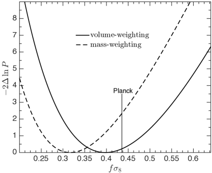
where ζm(fσ8)superscript𝜁m𝑓subscript𝜎8\zeta^{\mathrm{m}}(f\sigma_{8}) is the model prediction obtained according to (35) using ξuδ1superscriptsubscript𝜉𝑢𝛿1{\xi}_{{}_{u\delta}}^{1} and ξuw1superscriptsubscript𝜉𝑢𝑤1{\xi}_{{}_{uw}}^{1} of the mocks. The covariance matrix Cmsuperscript𝐶mC^{\mathrm{m}} depends on fσ8𝑓subscript𝜎8f\sigma_{8} through the cosmic variance term which is also extracted from the mocks assuming it has the same fσ𝑓𝜎f\sigma scaling as the correlations. Since we are using linear theory to model the dependence on fσ8𝑓subscript𝜎8f\sigma_{8}, we limit the calculation of χ2superscript𝜒2\chi^{2} in (6.2) to large scales, including only the 7 points with separations larger than 15h1Mpcsuperscript1Mpch^{-1}\,{\rm Mpc}. Further, we take σ8g0.93±0.05superscriptsubscript𝜎8gplus-or-minus0.930.05\sigma_{8}^{\mathrm{g}}\approx 0.93\pm 0.05 (cf. §5) in (35). Figure 3 plots curves of 2ΔlnP=2lnP+2ln[max(P)]2Δln𝑃2ln𝑃2lndelimited-[]max𝑃-2\Delta{\rm ln}P=-2{\rm ln}P+2{\rm ln}[\mathrm{max}(P)] for the volume and mass weighting schemes, as indicated in the figure. Minima of 2ΔlnP2Δln𝑃-2\Delta{\rm ln}P are rendered at the best fit values of fσ8𝑓subscript𝜎8f\sigma_{8} and and 2ΔlnP=12Δln𝑃1-2\Delta{\rm ln}P=1 mark the corresponding 1σ1𝜎1\sigma errors. We find

fσ8={0.40±0.08for ζV0.32±0.07for ζM𝑓subscript𝜎8casesplus-or-minus0.400.08for superscript𝜁𝑉otherwiseotherwiseplus-or-minus0.320.07for superscript𝜁𝑀f\sigma_{8}=\begin{cases}0.40\pm 0.08&\text{for }\zeta^{V}\\ &\\ 0.32\pm 0.07&\text{for }\zeta^{M}\end{cases} (37)

which are both consistent with the Planck value fσ8=0.43𝑓subscript𝜎80.43f\sigma_{8}=0.43. These estimates can be expressed in terms of βf/b=fσ8/σ8g𝛽𝑓𝑏𝑓subscript𝜎8superscriptsubscript𝜎8g\beta\equiv f/b=f\sigma_{8}/\sigma_{8}^{\mathrm{g}}. For σ8g=0.93±0.05superscriptsubscript𝜎8gplus-or-minus0.930.05\sigma_{8}^{\mathrm{g}}=0.93\pm 0.05 we obtain,

β={0.43±0.09for ζV0.34±0.08for ζM𝛽casesplus-or-minus0.430.09for superscript𝜁𝑉otherwiseotherwiseplus-or-minus0.340.08for superscript𝜁𝑀\beta=\begin{cases}0.43\pm 0.09&\text{for }\zeta^{V}\\ &\\ 0.34\pm 0.08&\text{for }\zeta^{M}\end{cases} (38)

The parameters obtained from the two curves are consistent at the 1σsimilar-toabsent1𝜎\sim 1\sigma level. It is tempting to derive parameters based on the joint measurements of ζVsuperscript𝜁𝑉\zeta^{V} and ζMsuperscript𝜁𝑀\zeta^{M}. Unfortunately, the number of mocks we have do not allow a robust estimation of the strong covariance between ζVsuperscript𝜁𝑉\zeta^{V} and ζMsuperscript𝜁𝑀\zeta^{M}. Attempts to do that with the current mocks, lead to a singular covariance matrix.
Refer to caption
Figure 3: Curves of 2ΔlnP2Δln𝑃-2\Delta{\rm ln}P (equation 6.2) versus fσ8𝑓subscript𝜎8f\sigma_{8} derived from the observed ζVsuperscript𝜁𝑉\zeta^{V} (solid) and ζMsuperscript𝜁𝑀\zeta^{M} (dashed).

6.3 vvvδvvv𝛿\kern-0.24994pt\hbox{$v$}\kern-5.20601pt\kern 0.50003pt\hbox{$v$}\kern-5.20601pt\kern-0.24994pt\raise 0.43304pt\hbox{$v$}-\delta correlations: preliminary assessment

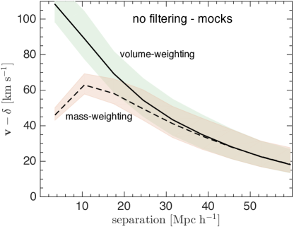
The 3D velocity is better correlated with the surrounding density fluctuations. This is mathematically evident by the expressions for 𝝃vvvδsubscript𝝃vvv𝛿{{\bm{\xi}}}_{{}_{\kern-0.12497pt\hbox{$v$}\kern-2.603pt\kern 0.25002pt\hbox{$v$}\kern-2.603pt\kern-0.12497pt\raise 0.21652pt\hbox{$v$}\delta}} and ξuδsubscript𝜉𝑢𝛿{\xi}_{{}_{u\delta}} in §3. Figure 4 illustrates this point. The solid and dashed curves are the dipole moments of the vvvδvvv𝛿\kern-0.24994pt\hbox{$v$}\kern-5.20601pt\kern 0.50003pt\hbox{$v$}\kern-5.20601pt\kern-0.24994pt\raise 0.43304pt\hbox{$v$}-\delta correlation from mocks, respectively, for volume and mass weighting schemes. The shaded areas are the corresponding cosmic variance and shot noise scatter. The curves are obtained in a similar way to the calculation of ζ𝜁\zeta for uδ𝑢𝛿u-\delta, as described in §4.3, with two differences: μβsubscript𝜇𝛽\mu_{\beta} is replaced with yyy^vvvα/vα^yyysubscriptvvv𝛼subscript𝑣𝛼\hat{\kern-0.24994pt\hbox{$y$}\kern-5.2616pt\kern 0.50003pt\hbox{$y$}\kern-5.2616pt\kern-0.24994pt\raise 0.43304pt\hbox{$y$}}\cdot\kern-0.24994pt\hbox{$v$}\kern-5.20601pt\kern 0.50003pt\hbox{$v$}\kern-5.20601pt\kern-0.24994pt\raise 0.43304pt\hbox{$v$}_{\alpha}/v_{\alpha} in (23) and uαsubscript𝑢𝛼u_{\alpha} is replaced with vαsubscript𝑣𝛼v_{\alpha} in both (24) and (25). Comparison with the uδ𝑢𝛿u-\delta correlations in the top panels in figure 2, clearly reveals a stronger vvvδvvv𝛿\kern-0.24994pt\hbox{$v$}\kern-5.20601pt\kern 0.50003pt\hbox{$v$}\kern-5.20601pt\kern-0.24994pt\raise 0.43304pt\hbox{$v$}-\delta signal for a similar width of the shaded areas.

The data provides the radial velocities and we need a method for inferring the underlying 3D velocity from sparse and noisy-data. Under the assumption of potential flow (Bertschinger & Dekel, 1989), the 3D velocity field can be reconstructed from the observed radial peculiar motions. Observational errors and incomplete spatial coverage in velocity catalogs limit the inference of the 3D flow to large scales only. We employ the methodology of Wiener filtering (Zaroubi et al., 1995) to reconstruct the 3D velocities. Given a set of measurements disubscript𝑑𝑖d_{i} at points rrrisubscriptrrr𝑖\kern-0.24994pt\hbox{$r$}\kern-4.78937pt\kern 0.50003pt\hbox{$r$}\kern-4.78937pt\kern-0.24994pt\raise 0.43304pt\hbox{$r$}_{i} (i=1N)𝑖1𝑁(i=1\cdots N) the Wiener filtered (WF) field of a desired signal, FWF(rrr)superscript𝐹WFrrrF^{\mathrm{WF}}(\kern-0.24994pt\hbox{$r$}\kern-4.78937pt\kern 0.50003pt\hbox{$r$}\kern-4.78937pt\kern-0.24994pt\raise 0.43304pt\hbox{$r$}) at any point r𝑟rr𝑟rr𝑟r is

FWF(rrr)=Ξrα𝒟αα1dαsuperscript𝐹WFrrrsubscriptΞ𝑟superscript𝛼subscriptsuperscript𝒟1𝛼superscript𝛼subscript𝑑𝛼F^{\mathrm{WF}}(\kern-0.24994pt\hbox{$r$}\kern-4.78937pt\kern 0.50003pt\hbox{$r$}\kern-4.78937pt\kern-0.24994pt\raise 0.43304pt\hbox{$r$})=\Xi_{r\alpha^{\prime}}{\mathcal{D}}^{-1}_{\alpha\alpha^{\prime}}d_{\alpha} (39)

where ΞΞ\Xi and 𝒟𝒟\mathcal{D} are the “data-data” and “data-signal” correlation matrices. For gaussian errors and a gaussian underlying signal, the field FWFsuperscript𝐹WFF^{\mathrm{WF}} renders a maximum in the probability P(F|data)𝑃conditional𝐹𝑑𝑎𝑡𝑎P(F|data) for F𝐹F given the data. In our case, F𝐹F is the 3D velocity field, v𝑣vv𝑣vv𝑣v, and d𝑑d represents the observed radial velocities u𝑢u. Therefore, Ξ=ξuvvvΞsubscript𝜉𝑢vvv\Xi={\xi}_{{}_{u\kern-0.12497pt\hbox{$v$}\kern-2.603pt\kern 0.25002pt\hbox{$v$}\kern-2.603pt\kern-0.12497pt\raise 0.21652pt\hbox{$v$}}} and 𝒟=ξuu+𝒩𝒟subscript𝜉𝑢𝑢𝒩\mathcal{D}={\xi}_{{}_{uu}}+\mathcal{N} where 𝒩𝒩\mathcal{N} is the (diagonal) error matrix of u𝑢u in cosmicflows-3. The calculation of these matrices is done using the expressions derived in §3, modified for velocities in the LG frame. Thus instead of ξuu=u(rrr)u(rrr~)subscript𝜉𝑢𝑢delimited-⟨⟩𝑢rrr𝑢~rrr{\xi}_{{}_{uu}}=\langle u(\kern-0.24994pt\hbox{$r$}\kern-4.78937pt\kern 0.50003pt\hbox{$r$}\kern-4.78937pt\kern-0.24994pt\raise 0.43304pt\hbox{$r$})u(\tilde{\kern-0.24994pt\hbox{$r$}\kern-4.78937pt\kern 0.50003pt\hbox{$r$}\kern-4.78937pt\kern-0.24994pt\raise 0.43304pt\hbox{$r$}})\rangle we consider (u(rrr)vvv(0)rrr^)(u(rrr~)vvv(0)rrr~^)delimited-⟨⟩𝑢rrrvvv0^rrr𝑢~rrrvvv0^~rrr\langle(u(\kern-0.24994pt\hbox{$r$}\kern-4.78937pt\kern 0.50003pt\hbox{$r$}\kern-4.78937pt\kern-0.24994pt\raise 0.43304pt\hbox{$r$})-\kern-0.24994pt\hbox{$v$}\kern-5.20601pt\kern 0.50003pt\hbox{$v$}\kern-5.20601pt\kern-0.24994pt\raise 0.43304pt\hbox{$v$}(0)\cdot\hat{\kern-0.24994pt\hbox{$r$}\kern-4.78937pt\kern 0.50003pt\hbox{$r$}\kern-4.78937pt\kern-0.24994pt\raise 0.43304pt\hbox{$r$}})(u(\tilde{\kern-0.24994pt\hbox{$r$}\kern-4.78937pt\kern 0.50003pt\hbox{$r$}\kern-4.78937pt\kern-0.24994pt\raise 0.43304pt\hbox{$r$}})-\kern-0.24994pt\hbox{$v$}\kern-5.20601pt\kern 0.50003pt\hbox{$v$}\kern-5.20601pt\kern-0.24994pt\raise 0.43304pt\hbox{$v$}(0)\cdot\hat{\tilde{\kern-0.24994pt\hbox{$r$}\kern-4.78937pt\kern 0.50003pt\hbox{$r$}\kern-4.78937pt\kern-0.24994pt\raise 0.43304pt\hbox{$r$}}})\rangle and similarly for ξuvvvsubscript𝜉𝑢vvv{\xi}_{{}_{u\kern-0.12497pt\hbox{$v$}\kern-2.603pt\kern 0.25002pt\hbox{$v$}\kern-2.603pt\kern-0.12497pt\raise 0.21652pt\hbox{$v$}}}. Im addition to v𝑣vv𝑣vv𝑣v, we also apply the WF methodology to derive the most probable real space density contrast field, δ𝛿\delta, given the cosmicflows-3 data. This is done by taking Ξ=ξuδΞsubscript𝜉𝑢𝛿\Xi={\xi}_{{}_{u\delta}} where the uδ𝑢𝛿u-\delta correlation is given in (13).

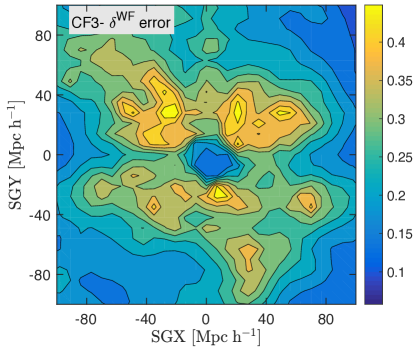
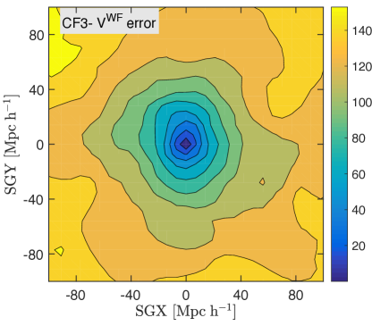
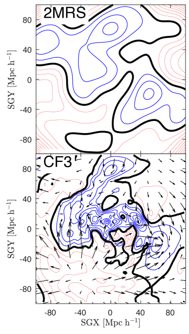
The WF 3D velocity, vvvWFsuperscriptvvvWF\kern-0.24994pt\hbox{$v$}\kern-5.20601pt\kern 0.50003pt\hbox{$v$}\kern-5.20601pt\kern-0.24994pt\raise 0.43304pt\hbox{$v$}^{\mathrm{WF}} and the corresponding density contrast, δWF=vvv/fsuperscript𝛿WFvvv𝑓\delta^{\mathrm{WF}}=-\kern-0.24994pt\hbox{$\nabla$}\kern-8.33336pt\kern 0.50003pt\hbox{$\nabla$}\kern-8.33336pt\kern-0.24994pt\raise 0.43304pt\hbox{$\nabla$}\cdot\kern-0.24994pt\hbox{$v$}\kern-5.20601pt\kern 0.50003pt\hbox{$v$}\kern-5.20601pt\kern-0.24994pt\raise 0.43304pt\hbox{$v$}/f on a uniform grid in the supergalactic plane (SGP) are shown in the bottom panel figure 5. The mean velocity in the SGP has been subtracted in order to emphasize the flow pattern in the plane. A comparison the WF reconstruction of Hoffman et al. (2015) for the cosmicflows-2 (Tully et al., 2013) catalog reveals a good general match. The Perseus-Pisces is apparent as an extended over-density in the bottom-right corner, Coma at the top, a horizontally elongated over-density from SGX=0𝑆𝐺𝑋0SGX=0 to SGX=80h1Mpc𝑆𝐺𝑋80superscript1MpcSGX=-80h^{-1}\,{\rm Mpc} at SGY0𝑆𝐺𝑌0SGY\approx 0 and a large void in the bottom left corner. The top panel shows contours of ln(1+δ)ln1𝛿{\rm ln}(1+\delta) obtained by smoothing the 2MRS galaxy distribution. There is a reasonable visual match between the δWFsuperscript𝛿WF\delta^{\mathrm{WF}} and the 2MRS density. While a constant smoothing is applied to the 2MRS, the WF filtering is a strong function of the errors and sparseness of the data. The agreement is satisfactory in light of the error map in figures 6&7. It is interesting that the errors in velocity increase with distance while decrease in the density.

Using vvvWFsuperscriptvvvWF\kern-0.24994pt\hbox{$v$}\kern-5.20601pt\kern 0.50003pt\hbox{$v$}\kern-5.20601pt\kern-0.24994pt\raise 0.43304pt\hbox{$v$}^{\mathrm{WF}}, we compute the dipole moment of the velocity density correlation. Volume and mass weighted dipole moments of vvvWFδsuperscriptvvvWF𝛿\kern-0.24994pt\hbox{$v$}\kern-5.20601pt\kern 0.50003pt\hbox{$v$}\kern-5.20601pt\kern-0.24994pt\raise 0.43304pt\hbox{$v$}^{\mathrm{WF}}-\delta are shown in the bottom panels of figure 2. The amplitude of the correlations, both in the data and the mocks, is substantially lower than the amplitude of the unfiltered vvvδvvv𝛿\kern-0.24994pt\hbox{$v$}\kern-5.20601pt\kern 0.50003pt\hbox{$v$}\kern-5.20601pt\kern-0.24994pt\raise 0.43304pt\hbox{$v$}-\delta correlations of in figure 4. The shaded areas representing shot-noise and cosmic variances corresponding to the vvvδvvv𝛿\kern-0.24994pt\hbox{$v$}\kern-5.20601pt\kern 0.50003pt\hbox{$v$}\kern-5.20601pt\kern-0.24994pt\raise 0.43304pt\hbox{$v$}-\delta correlation and shown in the bottom panels of Figure 2 are broader than in the top panels for the uδ𝑢𝛿u-\delta. This may seem surprising since a stronger correlation is expected for the 3D velocity. The reason for that is that the derivation of the 3D velocity is associated with an interpolation of the radial velocity data to all spaces. This effectively introduces additional source of error, as also seen in figures 6&7.

At separations >15h1Mpcsuperscriptsimilar-toabsent15superscript1Mpc\lower 2.15277pt\hbox{$\;\buildrel>\over{\sim}\;$}15h^{-1}\,{\rm Mpc}, the data and the mock correlations are in very good agreement for the volume-weighted correlation (left panel). The overall data correlation is below the mock curve in the mass weighting scheme (right panel). However, there is an important caveat in this comparison between data and mocks. The WF introduces a specific form of smoothing which depends on the specific spatial distribution of data points. To achieve an equivalent smoothing in the mocks, the cosmicflows-3 data points are padded in each mock and assigned the radial peculiar velocities of the nearest respective mock galaxies. Gaussian random scatter is then added according to the error estimate in the cosmicflows-3. This padding of data points in the mocks is done only for the purpose of vvvδvvv𝛿\kern-0.24994pt\hbox{$v$}\kern-5.20601pt\kern 0.50003pt\hbox{$v$}\kern-5.20601pt\kern-0.24994pt\raise 0.43304pt\hbox{$v$}-\delta correlation. It ensures identical WF window for mocks as in data but misses the correspondence between the selection of galaxies in the cosmicflows-3 and the underlying mass density. More galaxies should be selected in regions of higher density where the flow is convergent, and vice versa. Thus the comparison presented here should only serve as a “proof of concept” motivating a more thorough analysis. A potentially fruitful path to proceed is to augment the vvvWFsuperscriptvvvWF\kern-0.24994pt\hbox{$v$}\kern-5.20601pt\kern 0.50003pt\hbox{$v$}\kern-5.20601pt\kern-0.24994pt\raise 0.43304pt\hbox{$v$}^{\mathrm{WF}} with the missing small scale power according to Hoffman & Ribak (1991). For Gaussian fields, this will yield the most likely unfiltered estimates of the 3D velocities, given the radial peculiar velocities.
Refer to caption
Figure 4: Dipole (l=1𝑙1l=1) moments of vvvδvvv𝛿\kern-0.24994pt\hbox{$v$}\kern-5.20601pt\kern 0.50003pt\hbox{$v$}\kern-5.20601pt\kern-0.24994pt\raise 0.43304pt\hbox{$v$}-\delta correlations derived from unfiltered peculiar velocities in the mocks.

Refer to caption
Figure 5: Top: Contour map of the natural logarithm of the 2MRS density field smoothed with a Gaussian window of 10h1Mpc10superscript1Mpc10h^{-1}\,{\rm Mpc} in width. Bottom: The velocity field vvvWFsuperscriptvvvWF\kern-0.24994pt\hbox{$v$}\kern-5.20601pt\kern 0.50003pt\hbox{$v$}\kern-5.20601pt\kern-0.24994pt\raise 0.43304pt\hbox{$v$}^{\mathrm{WF}} overlaid on maps of δWF=vvvWF/fsuperscript𝛿WFsuperscriptvvvWF𝑓\delta^{\mathrm{WF}}=-\kern-0.24994pt\hbox{$\nabla$}\kern-8.33336pt\kern 0.50003pt\hbox{$\nabla$}\kern-8.33336pt\kern-0.24994pt\raise 0.43304pt\hbox{$\nabla$}\cdot\kern-0.24994pt\hbox{$v$}\kern-5.20601pt\kern 0.50003pt\hbox{$v$}\kern-5.20601pt\kern-0.24994pt\raise 0.43304pt\hbox{$v$}^{\mathrm{WF}}/f, obtained by Wiener filtering of cosmicflows-3. Arrow lengths are proportional to the amplitude of the velocity where the arrow nearest to the bottom-left corner corresponds to 360kms1360kmsuperscripts1360\ {\rm km\,s^{-1}}. Both panels show fields in the supergalactic plane and the contour spacing is 0.250.250.25. Black, blue and red contours correspond to zero, positive and negative density contrast, respectively.

Refer to caption
Figure 6: Map of the expected 1σ1𝜎1\sigma error in δWFsuperscript𝛿WF\delta^{\mathrm{WF}}.
Refer to caption
Figure 7: Map of the expected 1σ1𝜎1\sigma error (in kms1kmsuperscripts1\ {\rm km\,s^{-1}}) in vvvWFsuperscriptvvvWF\kern-0.24994pt\hbox{$v$}\kern-5.20601pt\kern 0.50003pt\hbox{$v$}\kern-5.20601pt\kern-0.24994pt\raise 0.43304pt\hbox{$v$}^{\mathrm{WF}}.

7 summary and discussion

Distance measurements are very challenging and the cosmicflows-3 catalog is under constant “quality control” by its observers. Ongoing improvements in the catalog are expected to reduce systematics, especially at large distances. Following private communications with the observers, we opted to limit the analysis to objects within czmax=10000kms1𝑐subscript𝑧max10000kmsuperscripts1cz_{\mathrm{max}}=10000\ {\rm km\,s^{-1}}. An attempt to compute the correlation including objects at cz>czmax𝑐𝑧𝑐subscript𝑧maxcz>cz_{\mathrm{max}} failed to reach converging results. As seen in figure 2, it is cosmic variance rather than random observational errors that constitute the main source of random uncertainty in uδ𝑢𝛿u-\delta. Suppression of cosmic variance requires a significant increase in the volume probed by velocity catalogs. The next cosmicflows-4 is expected to have a better control of systematics, allowing us to use data at larger distances with greater confidence. Another important likely development is the likely HI SKA precursor telescopes (e.g. Blyth, 2015), which could potentially provide Tully-Fisher distances for tens of thousands of galaxies within 300h1Mpc300superscript1Mpc300h^{-1}\,{\rm Mpc}.

It is encouraging that the constraints derived here are consistent with other estimates based on 2MASS galaxies (e.g. Pike & Hudson, 2005; Erdogdu et al., 2005; Lavaux et al., 2008; Bilicki et al., 2011; Branchini et al., 2012). In particular, the detailed analysis of Davis et al. (2011) have demonstrated an excellent alignment between the velocity field from the SFI++ catalog of peculiar velocities and the gravitational force field obtained from the Ks=11.25subscript𝐾𝑠11.25K_{s}=11.25 2MRS of 2300similar-toabsent2300{\sim}2300 galaxies. The alignment is best for β=0.33±0.045𝛽plus-or-minus0.330.045\beta=0.33\pm 0.045 which is in excellent agreement with both β=0.34±0.08𝛽plus-or-minus0.340.08\beta=0.34\pm 0.08 (mass weighting) and β=0.43±0.09𝛽plus-or-minus0.430.09\beta=0.43\pm 0.09 (volume weighting). This is perhaps not surprising since cosmicflows-3 relies heavily on the SFI++ and the Ks=11.75subscript𝐾𝑠11.75K_{s}=11.75 2MRS is selected from the same galaxy population as the Ks=11.25subscript𝐾𝑠11.25K_{s}=11.25. Still the agreement is impressive given the different methodologies.

Velocity-density correlations play a role in the modeling of redshift distortions in the density auto correlation function as estimated from redshift surveys (Koda et al., 2014; Okumura et al., 2014; Sugiyama et al., 2015). Thus the analysis presented here could be useful since it provides direct observational constraints on these correlations.

Velocity-velocity (uu𝑢𝑢u-u) correlations can be computed directly from peculiar velocity catalogs. Galaxy motions are unbiased tracers of the underlying velocity field. Thus, in principle, uu𝑢𝑢u-u correlations are independent of galaxy bias, unlike uδ𝑢𝛿u-\delta correlations. However, in practice uu𝑢𝑢u-u correlations are affected by the distribution of objects in the velocity catalog. Further, they are prone to larger cosmic variance uncertainties (Hellwing et al., 2017). Therefore, uδ𝑢𝛿u-\delta correlations may prove more robust and useful.

Peculiar velocities induce spatial modulations of the observed galaxy luminosity function (when redshifts are used to transform fluxes to luminosities). Thus spatial luminosity variations could serve as a probe of peculiar motions (Tammann et al., 1979; Nusser et al., 2011; Feix et al., 2015, 2017). Thus useful information could be extracted by correlating spatial deviations from the global luminosity function on one hand and the surrounding galaxy distribution on the other. This particular application of the luminosity modulation method could be susceptible to environmental dependences of the luminosity function. Nevertheless, the application should at least yield upper limits on the amplitude of the correlations.

While this paper is in the production stages, Adams & Blake (2017) presented an analysis of the density-velocity covariance to improve cosmological constraints using 6dF data (Jones et al., 2004).

acknowledgments

The author thanks Enzo Branchini, Marc Davis, Maciek Bilicki and Wojtek Hellwing for useful comments. This research was supported by the I-CORE Program of the Planning and Budgeting Committee, THE ISRAEL SCIENCE FOUNDATION (grants No. 1829/12 and No. 203/09) and the Asher Space Research Institute.

References

  • Adams & Blake (2017) Adams C., Blake C., 2017, arXiv:1706.05205
  • Bertschinger & Dekel (1989) Bertschinger E., Dekel A., 1989, ApJ, 336, L5
  • Bilicki et al. (2011) Bilicki M., Chodorowski M., Jarrett T., Mamon G., 2011, ApJ, 741, 31
  • Blyth (2015) Blyth S. L., 2015, in Proc. Sci.. pp 496–499 (arXiv:1109.5605), doi:10.1017/S1743921312009702, http://arxiv.org/abs/1109.5605http://dx.doi.org/10.1017/S1743921312009702
  • Branchini et al. (2012) Branchini E., Davis M., Nusser A., 2012, MNRAS, 424, 472
  • Carrick et al. (2015) Carrick J., Turnbull S. J., Lavaux G., Hudson M. J., 2015, MNRAS, 450, 317
  • Ciecielag & Chodorowski (2004) Ciecielag P., Chodorowski M., 2004, MNRAS, 349, 945
  • Davis & Huchra (1982) Davis M., Huchra J., 1982, ApJ, 254, 437
  • Davis et al. (2011) Davis M., Nusser A., Masters K. L., Springob C., Huchra J. P., Lemson G., 2011, MNRAS, 413, 2906
  • Erdogdu et al. (2005) Erdogdu P., et al., 2005, MNRAS, 368, 1515
  • Feix et al. (2015) Feix M., Nusser A., Branchini E., 2015, Phys. Rev. Lett., 115, 011301
  • Feix et al. (2017) Feix M., Branchini E., Nusser A., 2017, MNRAS, 467, 468
  • Gorski (1988) Gorski K., 1988, ApJ, 332, L7
  • Hellwing et al. (2016) Hellwing W. A., Schaller M., Frenk C. S., Theuns T., Schaye J., Bower R. G., Crain R. A., 2016, MNRAS, 461, L11
  • Hellwing et al. (2017) Hellwing W. A., Nusser A., Feix M., Bilicki M., 2017, MNRAS, 467, 2787
  • Hoffman & Ribak (1991) Hoffman Y., Ribak E., 1991, ApJL, 380, L5
  • Hoffman et al. (2015) Hoffman Y., Courtois H. M., Brent Tully R., 2015, MNRAS, 449, 4494
  • Huchra et al. (2012) Huchra J., et al., 2012, ApJS, 199, 26
  • Jones et al. (2004) Jones D. H., et al., 2004, MNRAS, 355, 747
  • Kaiser (1988) Kaiser N., 1988, MNRAS, 231, 149
  • Keselman & Nusser (2016) Keselman A., Nusser A., 2016, MNRAS, 467, 1915
  • Koda et al. (2014) Koda J., et al., 2014, MNRAS, 445, 4267
  • Kogut et al. (1993) Kogut A., et al., 1993, ApJ, 419, 1
  • Lavaux et al. (2008) Lavaux G., Tully R. B., Mohayaee R., Colombi S., 2008, ApJ, 709, 483
  • Linder (2005) Linder E. V., 2005, Phys. Rev. D, 72, 043529
  • Lynden-Bell et al. (1988) Lynden-Bell D., Faber S. M., Burstein D., Davies R. L., Dressler A., Terlevich R. J., Wegner G., 1988, ApJ, 326, 19
  • Lynden-Bell et al. (1989) Lynden-Bell D., Lahav O., Burstein D., 1989, MNRAS, 241, 325
  • Nusser & Davis (1994) Nusser A., Davis M., 1994, ApJL, 421, L1
  • Nusser & Davis (1995) Nusser A., Davis M., 1995, MNRAS, 276, 1391
  • Nusser & Davis (2011) Nusser A., Davis M., 2011, ApJ, 736, 93
  • Nusser et al. (2011) Nusser A., Branchini E., Davis M., 2011, ApJ, 735
  • Nusser et al. (2014) Nusser A., Davis M., Branchini E., 2014, ApJ, 788, 157
  • Okumura et al. (2014) Okumura T., Seljak U., Vlah Z., Desjacques V., 2014, JCAP, 2014, 003
  • Peebles (1980) Peebles P. J. E., 1980, The large-scale structure of the universe. Princeton University Press, NJ, http://adsabs.harvard.edu/abs/1980lssu.book.....P
  • Pike & Hudson (2005) Pike R. W., Hudson M. J., 2005, ApJ, 635, 11
  • Planck Collaboration et al. (2016) Planck Collaboration et al., 2016, A&A, 594, A13
  • Sachs & Wolfe (1967) Sachs R., Wolfe A., 1967, ApJ, 147, 73
  • Schmoldt et al. (1999) Schmoldt I., et al., 1999, MNRAS, 304, 893
  • Skillman et al. (2014) Skillman S. W., Warren M. S., Turk M. J., Wechsler R. H., Holz D. E., Sutter P. M., 2014, Arxiv:1407.2600, p. 26
  • Springob et al. (2007) Springob C., Masters K., Haynes M., Giovanelli R., Marinoni C., 2007, apjs, 172, 599
  • Strauss & Davis (1988) Strauss M., Davis M., 1988, in , Large-Scale Motions Universe A Vatican study Week. Princeton University Press, NJ, pp 255–274
  • Strauss & Willick (1995) Strauss M., Willick J., 1995, Physics Reports, 261, 271
  • Sugiyama et al. (2015) Sugiyama N. S., Okumura T., Spergel D. N., 2015, JCAP, 7, 18
  • Tammann et al. (1979) Tammann G., Yahil A., Sandage A., 1979, ApJ, 234, 775
  • Tully et al. (2013) Tully R. B., et al., 2013, ApJ, 146, 86
  • Tully et al. (2016) Tully R. B., Courtois H. M., Sorce J. G., 2016, Astron. J., 152, 1
  • Turner (1979) Turner E. L., 1979, Astrophys. J., 231, 645
  • Watkins & Feldman (2014) Watkins R., Feldman H. A., 2014, MNRAS, 450, 1868
  • Westover (2007) Westover M., 2007, PhD thesis, Harvard University
  • Zaroubi et al. (1995) Zaroubi S., Hoffman Y., Fisher K., Lahav O., 1995, ApJ, 449, 446