Abstract

We consider recursive decoding for Reed-Muller (RM) codes and their subcodes. Two new recursive techniques are described. We analyze asymptotic properties of these algorithms and show that they substantially outperform other decoding algorithms with nonexponential complexity known for RM codes. Decoding performance is further enhanced by using intermediate code lists and permutation procedures. For moderate lengths up to 512, near-optimum decoding with feasible complexity is obtained.

Keywords: Recursive decoding, Reed-Muller codes, decoding threshold, Plotkin construction, permutations.

1 Introduction

Below we consider Reed-Muller (RM) codes and their subcodes. We use notation $\left\{\genfrac{}{}{0.0pt}{}{m}{r}\right\}$ for RM codes of length $n=2^{m},$ dimension $k=\sum_{i=0}^{r}{\binom{m}{i}}$ and distance $d=2^{m-r}$. In this paper, we wish to design fast decoding algorithms that outperform other algorithms known for RM codes. To achieve this goal, we will use recursive techniques that make decoding decisions by combining decoding results obtained on the shorter codes.

RM codes are almost on par with the best codes on moderate lengths $n\leq 128$ and have found numerous applications thanks to fast decoding procedures. First, majority algorithm was developed in [1] followed later by numerous developments. Such a decoding has low complexity of the order $nk$ and enables bounded distance decoding.

It is also important that majority decoding substantially extends bounded-distance threshold of $d/2.$ Given an infinite sequence of codes $A_{i}(n_{i},d_{i}),$ we say that a decoding algorithm $\Psi$ achieves decoding thresholds $\delta_{i}$ if for any $\epsilon>0$ only a vanishing fraction of error patterns of weight $\delta_{i}(1-\epsilon)$ is left uncorrected as $n_{i}\rightarrow\infty.$ It can be proven [5] that majority algorithm achieves a threshold

$$\delta=(d\ln d)/4\$$ (1)

for long RM codes of fixed rate $R$ (here and below we omit index $i$). For long low-rate RM codes of fixed order $r$, it is shown [11] that majority decoding achieves a threshold

$$\delta=n(1-\varepsilon_{r}^{\text{maj}})/2,$$

where the residual term $\varepsilon_{r}^{\text{maj}}$ has a slowly declining order

$$\varepsilon_{r}^{\text{maj}}\sim(m/d)^{1/2^{r+1}}=(m/2^{m-r})^{1/2^{r+1}},\quad m\rightarrow\infty.$$ (2)

Therefore $\delta$ exceeds bounded distance threshold $d/2$ approximately $2^{r}$ times and approaches the upper limit of $n/2$ for long codes.

Another efficient technique is based on recursive algorithms of [2] and [3]. The recursive structure of RM codes $\left\{\genfrac{}{}{0.0pt}{}{m}{r}\right\}$ is well known [4] and is formed by the Plotkin construction $(\mathbf{u,u+v}),$ where subblocks $\mathbf{u}$ and $\mathbf{v}$ are taken from the codes $\left\{\genfrac{}{}{0.0pt}{}{m-1}{r}\right\}$ and $\left\{\genfrac{}{}{0.0pt}{}{m-1}{r-1}\right\}$. It is proven in [2] and [3] that this recursive structure allows to execute bounded distance decoding with the lowest complexity order of $n\min(r,m-r)$ known for RM codes. The techniques developed below also show that recursive algorithms of [2] and [3] are on par with majority decoding and achieve the same error-correcting thresholds $\delta$ in both cases (1) and (2).

One more efficient algorithm based on permutation decoding was designed in [6] for RM codes $\left\{\genfrac{}{}{0.0pt}{}{m}{2}\right\}$. This algorithm gives a slightly higher complexity order of $n^{2}m$ while reducing the corresponding residual term $\varepsilon_{2}^{\text{maj}}$ from (2) to the lower order of $(m/n)^{1/4}$ as $m\rightarrow\infty.$

The above algorithms can also be extended for soft decision channels. For RM codes of fixed rate $R,$ soft decision majority decoding [11] gives a threshold of Euclidean weight $\rho=(n/m)^{1/2^{r+1}}\sqrt{n}$. Using technique of [11], it can be proven that recursive algorithms of [2] and [3] also have the same error-correcting threshold $\rho.$ For RM codes $\left\{\genfrac{}{}{0.0pt}{}{m}{2}\right\}$, the algorithm of [6] allows to increase the Euclidean threshold $\rho$ to the order of $(n/m)^{1/4}\sqrt{n}.$ Finally, multistage maximum-likelihood decoding is performed in [7] by designing an efficient multilevel trellis structure. ML decoding supersedes recursive algorithms. In particular, it can be proven (similarly to [6]) that ML decoding has Euclidean threshold upper bounded by the order of $n\sqrt{(r!\ln 2)/2m^{r}}.$ However, ML decoding complexity is exponential in $n$.

Below we design new recursive algorithms that substantially outperform other (nonexponential) algorithms known for RM codes for both hard and soft decision channels. Our basic recursive procedure will split the RM code $\left\{\genfrac{}{}{0.0pt}{}{m}{r}\right\}$ of length $n$ into two RM codes of length $n/2$. Decoding is then relegated further to the shorter codes until we reach basic codes and perform ML decoding with complexity $O(n\log n).$ In all intermediate steps, we only recalculate the reliabilities of the newly defined symbols.

Below in Section 2 we consider recursive structure of RM codes in more detail. Then in Sections 3 and 4 we proceed with decoding techniques and design two different versions $\Psi_{r}^{m}$ and $\Phi_{r}^{m}$ of our recursive algorithm. In Section 5 we proceed with further improvements. In particular, decoding performance will be considerably improved by using subcodes of RM codes. Another improvement is based on using relatively short lists of codewords in the intermediate steps of the recursion. Finally, we use different permutations taken from the symmetry (automorphism) group of the code. As a result, we closely approach ML decoding performance on the blocklength of 256 and for low-rate codes of length 512.

2 Recursive structure

Recursive techniques known for RM codes are based on the Plotkin construction. Here any RM code $\left\{\genfrac{}{}{0.0pt}{}{m}{r}\right\}$ is represented in the form $(\mathbf{u,u+v}),$ where $\mathbf{u}$ and $\mathbf{v}$ are two subblocks of length $2^{m-1}$ that run through the codes $\left\{\genfrac{}{}{0.0pt}{}{m-1}{r}\right\}$ and $\left\{\genfrac{}{}{0.0pt}{}{m-1}{r-1}\right\},$ respectively. By continuing this process on codes $\left\{\genfrac{}{}{0.0pt}{}{m-1}{r}\right\}$ and $\left\{\genfrac{}{}{0.0pt}{}{m-1}{r-1}\right\},$ we obtain RM codes of length $2^{m-2}$ and so on. Finally, we arrive at the end nodes, which are repetition codes $\left\{\genfrac{}{}{0.0pt}{}{g}{0}\right\}$ for any $g=1,\ldots,m-r$ and full spaces $\left\{\genfrac{}{}{0.0pt}{}{h}{h}\right\}$ for any $h=1,\ldots,r.$ This is schematically shown in Fig. 1 for RM codes of length 16. In Fig. 2, we consider incomplete decomposition for codes of length 32 terminated at the biorthogonal codes and single-parity check codes.

0,0                                                     2,1

$\nearrow$ $\ \nwarrow$                                                 $\nearrow$ $\ \nwarrow$

1,0      1,1                                           3,1       3,2

$\ \ \ \ \ \ \ \ \ \ \ \ \ \ \ \ \ \ \ \ \ \ \nearrow$  $\nwarrow$    $\nearrow$ $\ \nwarrow$ $\ \ \ \ \ \ \ \ \ \ \ \ \ \ \ \ \ \ \ \ \ \ \ \ \ \ \ \ \ \ \ \ \ \ \ \ \nearrow$  $\nwarrow$    $\nearrow$ $\ \nwarrow$

2,0       2,1        2,2                                4,1        4,2       4,3        

$\nearrow$ $\ \nwarrow$    $\nearrow$ $\ \nwarrow$    $\nearrow$ $\ \nwarrow$                        $\nearrow$ $\ \nwarrow$    $\nearrow$ $\ \nwarrow$    $\nearrow$ $\ \nwarrow$

3,0      3,1        3,2       3,3                      5,1      5,2        5,3      5,4 

$\nearrow$ $\ \nwarrow$    $\nearrow$ $\ \nwarrow$    $\nearrow$ $\ \nwarrow$    $\nearrow$ $\ \nwarrow$

4,0       4,1        4,2        4,3       4,4       

Fig. 1$:$ Full decomposition          Fig. 2$:$ Partial decomposition

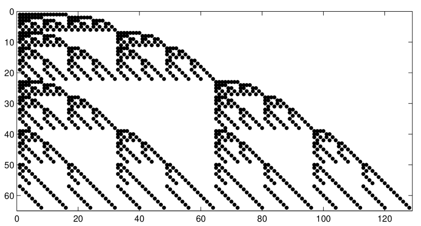
This recursive structure is also exhibited in the generator matrices of RM codes. As an example, on Fig. 3 we present a generator matrix for $\left\{\genfrac{}{}{0.0pt}{}{7}{3}\right\}$ code.

Figure 3: A generator matrix of $\left\{\genfrac{}{}{0.0pt}{}{7}{3}\right\}$ code. Ones are denoted by dots, zeroes are not shown.

Now let $\mathbf{a}\genfrac{}{}{0.0pt}{}{m}{r}=\{a_{j}|j=1,k\}$ be a block of information bits $a_{j}$ that encodes a vector $(\mathbf{u},\mathbf{u}+\mathbf{v}).$ Then recursive procedure splits $\mathbf{a}\genfrac{}{}{0.0pt}{}{m}{r}$ into two information subblocks $\mathbf{a}\genfrac{}{}{0.0pt}{}{m-1}{r}$ and $\mathbf{a}\genfrac{}{}{0.0pt}{}{m-1}{r-1}$ that encode vectors $\mathbf{u}$ and $\mathbf{v,}$ respectively. In this way, information subblocks are split until we arrive at the end nodes. Thus, any specific codeword can be encoded from the information strings assigned to the end nodes $\left\{\genfrac{}{}{0.0pt}{}{g}{0}\right\}$ or $\left\{\genfrac{}{}{0.0pt}{}{h}{h}\right\}$.

Also, it can be proven that recursive encoding of code $\left\{\genfrac{}{}{0.0pt}{}{m}{r}\right\}$ has complexity

$$\psi_{r}^{m}\leq n\min(r,m-r).$$ (3)

This observation comes from the two facts. First, the end nodes $\left\{\genfrac{}{}{0.0pt}{}{g}{0}\right\}$ and $\left\{\genfrac{}{}{0.0pt}{}{h}{h}\right\}$ satisfy the complexity bound (3). Second, we can obtain an $(\mathbf{u,u+v})$-codeword using two constituent codewords taken from $\left\{\genfrac{}{}{0.0pt}{}{m-1}{r-1}\right\}$ and $\left\{\genfrac{}{}{0.0pt}{}{m-1}{r}\right\}$. Therefore the overall complexity satisfies inequality $\psi_{r}^{m}\leq\psi\genfrac{}{}{0.0pt}{}{m-1}{r-1}+\psi\genfrac{}{}{0.0pt}{}{m-1}{r}+\frac{n}{2}$. Now we see that code $\left\{\genfrac{}{}{0.0pt}{}{m}{r}\right\}$ satisfies (3) if the two constituent codes do. In particular, for $r<m/2,$ we obtain the bound

$$\psi_{r}^{m}\leq n(r-1)/2+nr/2+n/2=nr.$$

Now consider an information bit $a_{j}$ associated with any left node, say $\left\{\genfrac{}{}{0.0pt}{}{g}{0}\right\}.$ Then splitting procedure also allows us to map this symbol $a_{j}$ onto a specific “binary path” $\overline{j}=(j_{1},\ldots,j_{m})$ leading from the origin $\left\{\genfrac{}{}{0.0pt}{}{m}{r}\right\}$ to the end node $\left\{\genfrac{}{}{0.0pt}{}{g}{0}\right\}$. To do this, we first take $j_{1}=0$ for any $a_{j}\in$ $\mathbf{a}\genfrac{}{}{0.0pt}{}{m-1}{r}$ and $j_{1}=1$ for $\mathbf{a}\genfrac{}{}{0.0pt}{}{m-1}{r-1}.$ On any step $s=2,\ldots,m$, we take $j_{s+1}=1$ when moving to the left (say, from $\mathbf{a}\genfrac{}{}{0.0pt}{}{m-1}{r-1}$ to $\mathbf{a}\genfrac{}{}{0.0pt}{}{m-2}{r-2}$ $)$ or $j_{s+1}=0$ when moving to the right. Then we get a subindex $=(j_{1},\ldots,j_{m-g})$ at the left-end node $\left\{\genfrac{}{}{0.0pt}{}{g}{0}\right\}$ associated with the information bit $a_{j}$. We complete this mapping by adding $g$ zeros $j_{m-g+1}=\cdots=j_{m}=0$ to $\overline{j}_{g}.$ As a result, we obtain the full path $\overline{j}$ that arrives at the node $\left\{\genfrac{}{}{0.0pt}{}{0}{0}\right\}.$

Now consider the right-end node $\left\{\genfrac{}{}{0.0pt}{}{h}{h}\right\}$ that includes $2^{h}$ information bits. In this case, the same mapping procedure gives a subpath $\overline{j}_{h}=(j_{1},\ldots,j_{m-h})$. To enumerate any specific information bit $a_{j}$ associated with this node $\left\{\genfrac{}{}{0.0pt}{}{h}{h}\right\}$, subindex $\overline{j}_{h}=(j_{1},\ldots,j_{m-h})$ is appended by any combination $(j_{m-h+1},\ldots,j_{m})$. As a result, we enumerate all $2^{h}$ bits $a_{j}$ given at the node $\left\{\genfrac{}{}{0.0pt}{}{h}{h}\right\}.$ It can also be seen that all indices $\{\overline{j}\}$ include at most $r$ ones in their binary representation. Therefore all $k$ information bits of the whole code are mapped onto $m$-digital binary paths $\overline{j}$ of weight $r$ or less.

3 New decoding techniques

Below we consider a new recursive algorithm $\Psi_{\text{rec}}$ based on the $(\mathbf{u,u+v})$ construction. The received block $\mathbf{y}=(\widetilde{\mathbf{u}},\widetilde{\mathbf{u+v}})$ consists of two halves $\mathbf{y}^{\prime}$ and $\mathbf{y}^{\prime\prime}$ corrupted by noise. By taking outputs $y_{i}^{\prime}$ and $y_{i}^{\prime\prime}$, the decoder finds the posterior probabilities of symbols $u_{i}$ and $u_{i}\mathbf{+}v_{i}:$

$$p_{i}^{\prime}\overset{\text{def}}{=}\Pr\{u_{i}=0\,\,|\,\,y_{i}^{\prime}\},\quad p_{i}^{\prime\prime}\overset{\text{def}}{=}\Pr\{u_{i}\mathbf{+}v_{i}=0\,\,|\,\,y_{i}^{\prime\prime}\},\quad i=1,\ldots,n/2.$$

We first try to find the better protected codeword $\mathbf{v}$ from $\left\{\genfrac{}{}{0.0pt}{}{m-1}{r-1}\right\}\mathbf{.}$ Then we decode the block $\mathbf{u\in}\left\{\genfrac{}{}{0.0pt}{}{m-1}{r}\right\}$.

Step 1. To find a subblock $\mathbf{v}$ in hard-decision decoding, one would use its corrupted version $\widetilde{\mathbf{v}}=\widetilde{\mathbf{u}}+\widetilde{\mathbf{u}+\mathbf{v}}.$ Using more general approach, we find $n/2$ posterior probabilities

$$p_{i}^{\mathbf{v}}\overset{\text{def}}{=}\Pr\{v_{i}=0\,\,|\,\,y_{i}^{\prime}\,,y_{i}^{\prime\prime}\}=p_{i}^{\prime}p_{i}^{\prime\prime}+(1-p_{i}^{\prime})(1-p_{i}^{\prime\prime}).$$ (4)

Here we apply the formula of total probability to the binary sum of independent symbols $u_{i}$ and $u_{i}\mathbf{+}v_{i}.$ Now we can use any soft-decision decoding $\Psi_{\mathbf{v}}(p_{i}^{\mathbf{v}})$ to find vector $\widehat{\mathbf{v}}$. This completes Step 1 of our algorithm. Vector $\widehat{\mathbf{v}}$ is then passed to Step 2.

Step 2. Now we use both symbols $y_{i}^{\prime\prime}$ and $v_{i}$ to estimate symbol $u_{i}$ on the right half. Assuming that $\widehat{\mathbf{v}}=\mathbf{v}$ , we find that symbol $u_{i}$ has posterior probability

$$p_{i}^{\wedge}\overset{\text{def}}{=}\Pr\{u_{i}=0\,\,|\,y_{i}^{\prime\prime},\,\widehat{v}_{i}\}=\left\{\begin{array}[c]{ll}p_{i}^{\prime\prime},&\text{if}\;\widehat{v}_{i}=0,\\ 1-p_{i}^{\prime\prime},&\text{if}\;\widehat{v}_{i}=1.\end{array}\right.$$

Now we have the two posterior probabilities $p_{i}^{\prime}$ and $p_{i}^{\wedge}$ of symbol $u_{i}$ obtained on both corrupted halves. By using the Bayes’ formula, we find the combined estimate

$$p_{i}^{\mathbf{u}}\overset{\text{def}}{=}\Pr\{u_{i}=0\,|\,\,p_{i}^{\prime},\,p_{i}^{\wedge}\}=\frac{p_{i}^{\prime}p_{i}^{\wedge}}{p_{i}^{\prime}p_{i}^{\wedge}+(1-p_{i}^{\prime})(1-p_{i}^{\wedge})}.$$ (5)

Finally, we perform soft decision decoding $\Psi_{\mathbf{u}}(p_{i}^{\mathbf{u}})$ and find a subblock $\widehat{\mathbf{u}}\mathbf{\in}\left\{\genfrac{}{}{0.0pt}{}{m-1}{r}\right\}.$ So, the basic soft-decision decoding $\Psi_{\text{rec}}$ uses procedures $\Psi_{\mathbf{v}}$, $\Psi_{\mathbf{u}}$ and outputs a decoded codeword $\mathbf{\hat{c}}$ and the corresponding information block $\widehat{\mathbf{a}}$ as follows.

In a more general scheme $\Psi_{r}^{m}$, we repeat this recursion by decomposing subblocks $\widehat{\mathbf{v}}$ and $\widehat{\mathbf{u}}$ further. On all intermediate steps, we only recalculate the probabilities of the newly defined symbols. Finally, we perform ML decoding once we reach the end nodes $\left\{\genfrac{}{}{0.0pt}{}{g}{0}\right\}$ and $\left\{\genfrac{}{}{0.0pt}{}{h}{h}\right\}$. The algorithm is described below.

In the next algorithm $\Phi_{r}^{m}$, we terminate decoding $\Psi_{\mathbf{v}}$ at the biorthogonal codes $\left\{\genfrac{}{}{0.0pt}{}{g}{1}\right\}$.

Thus, procedures $\Psi_{r}^{m}$ and $\Phi_{r}^{m}$ have recursive structure that calls itself until ML decoding is applied on the end nodes. ML decoding of biorthogonal codes has complexity order of $n\log_{2}n$. Simple analysis also shows that recalculating all posterior probabilities in (4) and (5) has complexity at most $5n.$ Therefore our decoding complexity $\Phi_{r}^{m}$ satisfies recursion

$$\Phi_{r}^{m}\leq\Phi_{r-1}^{m-1}+\Phi_{r}^{m-1}+5n.$$

Similarly to the derivation of (3), this recursion brings the overall complexity of $\Phi_{r}^{m}$ and $\Psi_{r}^{m}$ to the order of $5n\log_{2}n$ real operations.

4 Analysis of algorithms $\Psi_{r}^{m}$ and $\Phi_{r}^{m}$.

In general, procedure $\Psi_{r}^{m}$ enters each end node by taking all paths leading to this node. It turns out that the output bit error rate (BER) significantly varies on different nodes and even on different paths leading to the same node. Therefore our first problem is to define the most error-prone paths.

Asymptotic analysis. We consider AWGN channels and assume that the all-zero codeword is transmitted as a sequence of $+1$s. Then $n$ outputs $y_{i}^{\prime}$ and $y_{i}^{\prime\prime}$ are independent random variables  (RV) with normal distribution $\mathcal{N}(1,\sigma^{2}).$ It can be readily seen that the posterior probabilities $p_{i}$ (that is $p_{i}^{\prime}$ or $p_{i}^{\prime\prime})$ become independent RV with non-Gaussian distribution

$$p_{i}=\frac{1}{2}(1+\varepsilon_{i}),\quad\text{where }\varepsilon_{i}=\tanh\frac{y_{i}}{\sigma^{2}},\quad\tanh(x)\triangleq\frac{e^{x}-e^{-x}}{e^{x}+e^{-x}}.$$ (6)

In the next step, we obtain the RV $p_{i}^{\mathbf{v}}$ and $p_{i}^{\mathbf{u}}.$ Here we rewrite equations (4) and (5) as follows.

Lemma 4.1

The values $p_{i}^{\mathbf{v}}$ and $p_{i}^{\mathbf{u}}$ can be calculated as

$$p_{i}^{\mathbf{v}}=\frac{1}{2}(1+\varepsilon_{i}^{\mathbf{v}}),\quad\varepsilon_{i}^{\mathbf{v}}=\varepsilon_{i}^{\prime}\varepsilon_{i}^{\prime\prime},$$ (7)

$$p_{i}^{\mathbf{u}}=\frac{1}{2}(1+\varepsilon_{i}^{\mathbf{u}}),\quad\varepsilon_{i}^{\mathbf{u}}=\tanh\frac{y_{i}^{\prime}+(-1)^{\widehat{v}_{i}}y_{i}^{\prime\prime}}{\sigma^{2}}.$$ (8)

The product RV $\varepsilon_{i}^{\mathbf{v}}$ defined in (7) has a smaller expected value relative to the original estimates $\varepsilon_{i}^{\prime}$ and $\varepsilon_{i}^{\prime\prime},$ since $0\leq\varepsilon_{i}^{\prime},\varepsilon_{i}^{\prime\prime}\leq 1$. Therefore the mean value of $p_{i}^{\mathbf{v}}$ converges to 0.5 in the subsequent left-hand steps. This makes decoding $\Psi_{\mathbf{v}}$ less reliable. On the positive side, we note that each step gives us a better protected code that has twice the relative distance of the former one. Therefore we subsequently degrade the channel while entering the new codes with higher correcting capabilities.

If $\widehat{v}_{i}$ is correct (i.e. $\widehat{v}_{i}=0$) we have $\varepsilon_{i}^{\mathbf{u}}=\tanh\{(y_{i}^{\prime}+y_{i}^{\prime\prime})/\sigma^{2}\}.$ So the second RV $\varepsilon_{i}^{\mathbf{u}}$ has a greater expected value. Consequently, the mean probabilities $p_{i}^{\mathbf{u}}$ increase as we move to the right. Note, however, that each new code has half the relative distance of its parent code. In other words, we subsequently improve the channel while entering the new codes with weaker correcting capabilities.

Now we proceed with an asymptotic analysis. We first consider RM codes with $m\rightarrow\infty$ and fixed order $r$. These codes have rates $R\rightarrow 0$. Therefore we have to consider the case $\sigma^{2}\rightarrow\infty$ to obtain any fixed signal-to-noise ratio $1/R\sigma^{2}$ as $m\rightarrow\infty.$ We will use the following lemma proven in [11].

Lemma 4.2

For large noise power $\sigma^{2}\rightarrow\infty$ the first two moments $E\varepsilon$ and $E\varepsilon^{2}$ of the random variable $\varepsilon=\tanh(y/\sigma^{2})$ satisfy the relation

$$E\varepsilon\sim E\varepsilon^{2}\sim\sigma^{-2}.$$ (9)

In general, we wish to use the original RV $y_{i},$ $\varepsilon_{i}^{\prime},$ and $\varepsilon_{i}^{\prime\prime}$ and recalculate their probability density functions (pdf), using (7) and (8) to find the pdf of the new RV variables $\varepsilon_{i}^{\mathbf{v}}$ and $\varepsilon_{i}^{\mathbf{u}}$. However, the latter formulas make these recalculations very involved. Therefore we consider a simplified version of our algorithm $\Psi_{\text{rec}}.$ Namely, given a channel symbol $y$ with posterior probability $p=(1+\varepsilon)/2,$ we define the likelihood of $0$

$$\rho(\varepsilon)\overset{\text{def}}{=}\frac{2y}{\sigma^{2}}=\ln\frac{1+\varepsilon}{1-\varepsilon}.$$

Note that the likelihoods form independent Gaussian RV. It can be easily seen that the new RV $\varepsilon_{i}^{\mathbf{u}}$ obtained in (8) gives the likelihood

$$\rho(\varepsilon_{i}^{\mathbf{u}})=\rho(\varepsilon_{i}^{\prime})+\rho(\varepsilon_{i}^{\prime\prime})$$ (10)

for any noise power $\sigma^{2}.$ For the RV $\varepsilon_{i}^{\mathbf{v}},$ the corresponding recalculation results in a longer formula

$$\rho(\varepsilon_{i}^{\mathbf{v}})=\ln\frac{1+\exp\rho(\varepsilon_{i}^{\prime})\exp\rho(\varepsilon_{i}^{\prime\prime})}{\exp\rho(\varepsilon_{i}^{\prime})+\exp\rho(\varepsilon_{i}^{\prime\prime})}.$$ (11)

Given the asymptotic case $\sigma^{2}\rightarrow\infty,$ note that the RV $\rho(\varepsilon_{i})$ takes small values with high probability. Therefore we replace the latter formula by its approximation valid for small $\rho(\varepsilon_{i}^{\prime})$ and $\rho(\varepsilon_{i}^{\prime\prime})$:

$$\rho(\varepsilon_{i}^{\mathbf{v}})\sim\rho(\varepsilon_{i}^{\prime})\rho(\varepsilon_{i}^{\prime\prime}).$$ (12)

It can be proven that the output bit error rate obtained on any end node $\left\{\genfrac{}{}{0.0pt}{}{g}{0}\right\}$ with large $g$ can be calculated using only the first two moments $E\rho$ and $E\rho^{2}$ of the RV $\rho=\rho(\varepsilon_{i}^{\mathbf{v}})$ obtained on this node. It can also be proven that the original formula (11) and its approximation (12) give the same moment $E\rho$ as $\sigma^{2}\rightarrow\infty.$ Also, the two formulas give the same asymptotic moments $E\rho^{2}.$ This justifies using the above approximation in the asymptotic case.

Now we consider a simplified algorithm $\Psi_{\text{rec}},$ with recalculations (7) and (8) replaced by (10) and (12). Using this simplified version $\Psi_{\text{rec}},$ we can arrive at the following conclusions [12].

Theorem 4.1

For $\sigma^{2}\rightarrow\infty$, replacing code $\left\{\genfrac{}{}{0.0pt}{}{m}{r}\right\}$ by $\left\{\genfrac{}{}{0.0pt}{}{m-1}{r-1}\right\}$ in the algorithm $\Psi_{\mathbf{v}}$ is equivalent to increasing the original noise power $\sigma^{2}$ to $\sigma^{4}$. Replacing code $\{\genfrac{}{}{0.0pt}{}{m}{r}\}$ by $\left\{\genfrac{}{}{0.0pt}{}{m-1}{r}\right\}$ in the algorithm $\Psi_{\mathbf{u}}$ reduces the original noise power $\sigma^{2}$ to $\sigma^{2}/2.$

Therefore in asymptotic setting our recursive procedure can be considered as a “propagation of the noise power”. This propagation undergoes two different types of changes while we move from the parent node to the two descendant nodes. This propagation is also illustrated on Fig. 4 as an example for the $\left\{\genfrac{}{}{0.0pt}{}{7}{3}\right\}$ code (note, however, that procedure becomes exact only for very long codes).

Now we can find asymptotic error rate for each bit (path) $a_{i}$. Note that algorithm $\Psi_{r}^{m}$ has the highest noise power $\sigma^{2^{r+1}}$ when it arrives at the leftmost (repetition) code $\left\{\genfrac{}{}{0.0pt}{}{m-r}{0}\right\}.$ Also, a repetition code of any length $n$ used on the AWGN channel $\mathcal{N}(0,\sigma^{2})$ has an output error probability of ML decoding

$$P=Q\left(\sqrt{n}/\sigma\right),\quad\text{where }Q(x)\triangleq\int_{x}^{\infty}e^{-u^{2}/2}\,du\,/\sqrt{2\pi}.$$ (13)

Note that for a general binary memoryless channel with noise variance $\sigma^{2},$ the same estimate can also be used on any node $\left\{\genfrac{}{}{0.0pt}{}{g}{0}\right\}$ given the following two conditions:

$$g\rightarrow\infty,\quad\sigma/2^{g/3}\rightarrow\infty.$$ (14)

Both conditions directly follow from the estimates obtained in [8] (p. 549) for the large deviations of the sums of independent random variables with common distribution.

Estimate (13) shows that the algorithm $\Psi_{r}^{m}$ gives the highest error rate

$$\mathcal{P}_{0}=Q\left(\sqrt{2^{m-r}}/\sigma^{2^{r}}\right)$$

on the leftmost node $\left\{\genfrac{}{}{0.0pt}{}{m-r}{0}\right\}$. The second highest error rate $\mathcal{P}_{1}=Q\left(\sqrt{2^{m-r+1}}/\sigma^{2^{r}}\right)$ is obtained on the next node $\left\{\genfrac{}{}{0.0pt}{}{m-r-1}{0}\right\}.$ Note that these probabilities rapidly decline. In particular, $\mathcal{P}_{1}\sim\mathcal{P}_{0}^{2}$ when $\mathcal{P}_{0}$ is small. In fact, for most noise powers $\sigma^{2},$ the first BER $\mathcal{P}_{0}$ exceeds all subsequent bit error rates so considerably that it practically defines the overall word ER (WER). By contrast, the lowest BER is obtained on the rightmost node $\left\{\genfrac{}{}{0.0pt}{}{m-r}{m-r}\right\}.$ Thus, we arrive at the following conclusions:

$\bullet$ The left-hand movement from a code $\left\{\genfrac{}{}{0.0pt}{}{j}{i}\right\}$ to the next code $\left\{\genfrac{}{}{0.0pt}{}{j-1}{i-1}\right\}$ increases the output BER. In this case, doubling the relative code distance $d/n$ does not compensate for a stronger noise obtained on the code $\left\{\genfrac{}{}{0.0pt}{}{j-1}{i-1}\right\}.$

$\bullet$ Moving to the right from a code $\left\{\genfrac{}{}{0.0pt}{}{j}{i}\right\}$ to the next code $\left\{\genfrac{}{}{0.0pt}{}{j-1}{i}\right\}$ allows us to reduce the BER of the algorithm relative to the parent code $\left\{\genfrac{}{}{0.0pt}{}{j}{i}\right\}$. As a result, the lowest BER is obtained on the rightmost node $\left\{\genfrac{}{}{0.0pt}{}{r}{r}\right\}.$

In a more general setting, we can estimate asymptotic error rates for any information bit $a_{j}$. For $c=0,1$ and $x>0,$ we use notation $x\diamond c\overset{\text{def}}{=}2^{1-c}x^{1+c}.$ Given a symbol $a_{j}$ arriving at the node $\left\{\genfrac{}{}{0.0pt}{}{g}{0}\right\}$ we can consider the corresponding subpath $\overline{j}_{g}=(j_{1},\ldots,j_{m-g})$. Then we define the product $x\diamond\overline{j}_{g}=(\cdots(x\diamond j_{1})\diamond j_{2}\cdots)\diamond j_{m-g}$ and arrive at the following statement.

Theorem 4.2

Consider RM codes with $m\rightarrow\infty$ and fixed order $r$. For the information bit $a_{j}$ associated with a node $\left\{\genfrac{}{}{0.0pt}{}{g}{0}\right\}$, algorithm $\Psi_{r}^{m}$ has bit error rate

$$\mathcal{P(}a_{j})\sim Q\left(\sigma\diamond\overline{j}_{g}\right),\quad g\rightarrow\infty.$$ (15)

Similar results hold for the algorithm $\Phi_{r}^{m}$, which stops at the nodes $\left\{\genfrac{}{}{0.0pt}{}{g}{1}\right\}$. This node is associated with a subblock of $g+1$ information bits. In this case the corresponding subindex $\overline{j}_{g}^{1}$ has weight $r-1$ or less. Therefore algorithm $\Phi_{r}^{m}$ reduces the highest noise power $\sigma^{2^{r+1}}$ to $\sigma^{2^{r}}$ and gives substantial improvement over $\Psi_{r}^{m}.$ More generally, we obtain the following statement.

Theorem 4.3

Consider RM codes with $m\rightarrow\infty$ and fixed order $r$. For the subset of $g+1$ information bits $\mathcal{\{}a_{j}\}$ associated with a node $\left\{\genfrac{}{}{0.0pt}{}{g}{1}\right\}$, algorithm $\Psi_{r}^{m}$ has bit error rate

$$\mathcal{P(\{}a_{j}\})\lesssim 2^{g}Q\left(\sigma\diamond\overline{j}_{g}^{1}\right),\quad g\rightarrow\infty.$$

In particular, the highest BER $\mathcal{P}_{0}$ obtained at the node $\left\{\genfrac{}{}{0.0pt}{}{m-r}{0}\right\}$ by $\Psi_{r}^{m}$ is now being replaced by

$$\mathcal{P}_{0}^{\prime}\lesssim 2^{m-r+1}Q\left(\sqrt{2^{m-r}}/\sigma^{2^{r-1}}\right)$$

obtained at the node $\left\{\genfrac{}{}{0.0pt}{}{m-r+1}{1}\right\}$. As the block length grows, decoding $\Phi_{r}^{m}$ increasingly outperforms both the majority algorithm and recursive techniques of [2], [3]. Further, this analysis can be extended to codes of fixed rate $R.$ In particular, the following statement holds for hard-decision decoding.

Theorem 4.4

For RM codes with $m\rightarrow\infty$ and fixed rate $R$, algorithm $\Phi_{r}^{m}$ has error-correcting threshold $(d\ln d)/2$ thus:

$\bullet$ increasing $\ln d$ times the threshold of bounded-distance decoding;

$\bullet$ doubling the threshold $(d\ln d)/4$ of majority decoding.

5 Improvements

1. Subcodes of RM codes

To improve output error rate, we set the leftmost information bits as zeros. In this way, we arrive at the subcodes of the original code $\left\{\genfrac{}{}{0.0pt}{}{m}{r}\right\}$ that are obtained by eliminating a few least protected information bits. This expurgation starts with the node $\left\{\genfrac{}{}{0.0pt}{}{m-r}{0}\right\}$ in procedure $\Psi_{r}^{m}$, and with the node $\left\{\genfrac{}{}{0.0pt}{}{m-r+1}{1}\right\}$ in $\Phi_{r}^{m}$. It can be shown that after eliminating only one bit, algorithm $\Psi_{r}^{m}$ gives the same BER on the channel whose noise power $\sigma^{2}$ is increased $2^{1/2^{r}}$ times. For the algorithm $\Phi_{r}^{m},$ the sustainable noise power is increased $2^{1/2^{r-1}}$ times. For long codes of small order $r=2,3$ this amounts to a gain of 1.5 dB and 0.75 dB, respectively.

2. List decoding

Decoding performance is further improved by choosing $L$ best candidates after each decoding step. This list decoding $\Psi_{r}^{m}(L)$ starts at the leftmost code $\left\{\genfrac{}{}{0.0pt}{}{m-r}{0}\right\}$. Here we define posterior probabilities $p(\mathbf{v}\mid\mathbf{y})$ of both codewords $\mathbf{v}^{\prime}=0$ and $\mathbf{v}^{\prime\prime}=1$. These codewords are represented as two initial edges with the corresponding cost functions $\log p(\mathbf{v}\mid\mathbf{y})$. Then we decode the next code $\left\{\genfrac{}{}{0.0pt}{}{m-r-1}{0}\right\}$. Note that codewords $\mathbf{v}$^′ and $\mathbf{v}^{\prime\prime}$ give different probability distributions on this node. Therefore our new decoding is performed 2 times, separately for $\mathbf{v}^{\prime}$ and $\mathbf{v}^{\prime\prime}\mathbf{.}$ The result is a full tree of depth 2 that has 4 new edges. On further steps, we keep doubling the number of paths until $2L$ paths are formed. Then we choose $L$ paths with maximum cost functions and proceed further. In the end, the most probable path (that has maximum cost function) is chosen among $L$ paths survived at the rightmost node. Simulation results and analytic estimates give very substantial improvements when both techniques – using the subcodes and short decoding lists – are combined. These results are presented below in Figures 5 to 8.

3. New permutation techniques

Finally, the third improvement utilizes the rich symmetry group $GA(m)$ of RM codes that includes $2^{O(m^{2})}$ permutations. First, note that even for large $L$ algorithm $\Psi_{r}^{m}(L)$ is likely to fail if error positions substantially disagree on the two halves of the original block. By using a symmetry group, we try to find the permutations that match unknown erroneous positions in the two permuted halves. If successful, procedure $\Psi_{\mathbf{v}}$ will eliminate most errors on the permuted block $\mathbf{v}$ of length $n/2.$ This process can be advanced in the next step, by finding another permutation that again gives a good match on erroneous positions left on the new halves of length $n/4.$

In particular, we use the following sets of permutations. Represent any position $i=1,\ldots,2^{m}$ in the binary form $i=(i_{1},\ldots,i_{m}).$ We take any permutation $\pi(1),\ldots,\pi(m)$ and consider the subgroup $S$ $\subset GA(m)$ that includes $m!$ permutations $(i_{1},\ldots,i_{m})\mapsto(i_{\pi(1)},\ldots,i_{\pi(m)}).$ Note that using subgroup $S$ also changes the “folding” order used in algorithm $\Psi_{\mathbf{v}}$ (say, we fold adjacent quarters instead of halves when we permute $i_{1}$ and $i_{2}).$ We can also consider $\left(\genfrac{}{}{0.0pt}{}{m}{r}\right)$ permutations taking exactly one permutation with a given subset $\pi^{-1}(1),\ldots,\pi^{-1}(r)$ of the first $r$ “folding” indices. Permutations from this subset $T$ change the order in which we decode left-end nodes. Finally, consider a subgroup $U$ that includes $m$ cyclic shifts $\pi(1),\ldots,\pi(m).$ Simulation results for the moderate lengths 256 and 512 showed that using subsets $T$ and even $U$ allows to reduce the combined list of $L$ best candidates by one decimal order. As a result, we obtained nearly ML decoding on the lengths 512 while using lists of moderate size $L.$

6 Simulation results

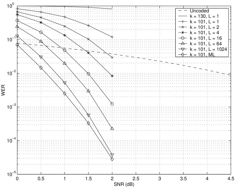
Simulation results are described in Figures 5 to 8. We start with Fig. 5

Figure 5: RM $\left\{\genfrac{}{}{0.0pt}{}{9}{3}\right\}$ code, $n=512$, $k=130$, and its subcode, $k=101$.

that reflects substantial improvements obtained when both techniques – using the subcodes and short decoding lists – were combined. The first (upper) curve with $L=1$ shows the performance of the algorithm $\Psi_{r}^{m}$ applied to the $\left\{\genfrac{}{}{0.0pt}{}{9}{3}\right\}$ code with $n=512$ and $k=130.$ This algorithm can be considered as a refined version of the former recursive techniques from [2], [3], and [10]. Namely, $\Psi_{r}^{m}$ uses exact probability recalculations presented in formulas (7) and (8) instead of various metrics used in these papers.

The second curve with $L=1$ shows the performance of the algorithm $\Psi_{r}^{m}$ applied to the $(512,101)$-subcode of the original $\left\{\genfrac{}{}{0.0pt}{}{9}{3}\right\}$ code. This subcode is obtained by removing 29 leftmost information bits with the highest BER. We see that the subcode gives substantial improvement in the output BER despite having a smaller code rate. All other curves on Fig. 5 correspond to the same subcode but use the bigger lists. We see from Fig. 5 that algorithm $\Psi_{r}^{m}$ is further improved by 3.5 to 5 dB at BER $10^{-4},$ by using the algorithm $\Psi_{r}^{m}(L)$ with moderate number $L$.

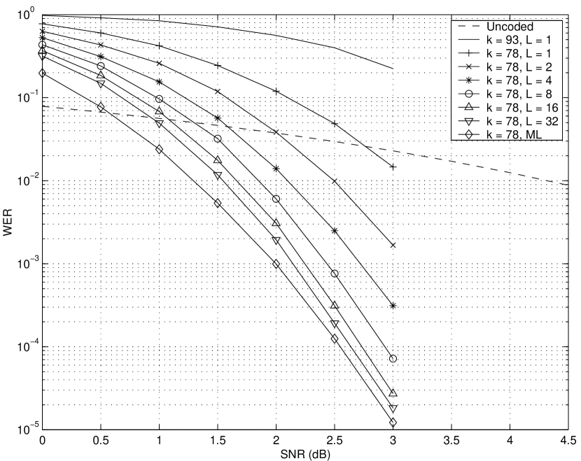
For large $L,$ simulation results (exhibited in Fig. 5 and 6)

Figure 6: RM $\left\{\genfrac{}{}{0.0pt}{}{8}{3}\right\}$ code, $n=256$, $k=93$, and its subcode, $k=78$.

also showed that most incorrectly decoded codewords are still more probable than the transmitted vector. This fact shows that our word ER (WER) is very close to that of ML decoding. In turn, this gives a new (experimental) bound on the WER of ML decoding.

It is also interesting that subcodes usually achieve near-ML decoding using much smaller lists relative to the original RM codes. In particular, Fig. 6 presents simulation results for a (256,78)-subcode of the (256,93)-code $\left\{\genfrac{}{}{0.0pt}{}{8}{3}\right\}$. This subcode approaches near-ML decoding using only 32 intermediate paths, while the original $\left\{\genfrac{}{}{0.0pt}{}{8}{3}\right\}$ requires about 512 paths (using permutation techniques) or even 4096 paths (without permutations). Note that even one of the most efficient algorithms developed in [9] uses about $10^{5}$ paths for BCH codes of length 256.

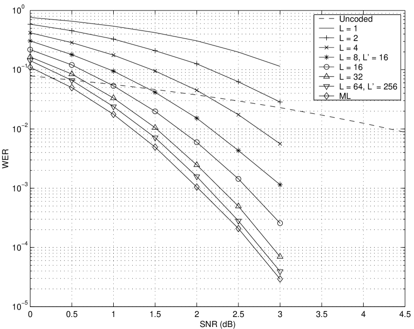
Fig. 7

Figure 7: RM $\left\{\genfrac{}{}{0.0pt}{}{8}{2}\right\}$ code, $n=256$, $k=37$. $L^{\prime}$ is the number of paths required to achieve approximately the same WER when no permutations are used.

presents simulation results when permutation techniques were applied to the $\left\{\genfrac{}{}{0.0pt}{}{8}{2}\right\}$ code with $n=256$ and $k=37.$ Here we compare the original recursive algorithm $\Psi_{r}^{m}(L)$ with its refined version that uses a small subgroup $U$ defined in the previous section. The results show that adding a few permutations can substantially reduce the overall list size (taken over all permutations). For this specific code, the refined version reduces approximately 4 times the number of trials used in $\Psi_{r}^{m}(L)$ to obtain near-ML decoding. Similar results show that for codes of length $512$ the complexity of near-ML decoding is reduced tenfold.

Finally, in Fig. 8,

Figure 8: Experimental lower bounds for RM $\left\{\genfrac{}{}{0.0pt}{}{8}{2}\right\},\ldots,\left\{\genfrac{}{}{0.0pt}{}{8}{6}\right\}$, and $\left\{\genfrac{}{}{0.0pt}{}{9}{2}\right\}$ codes.

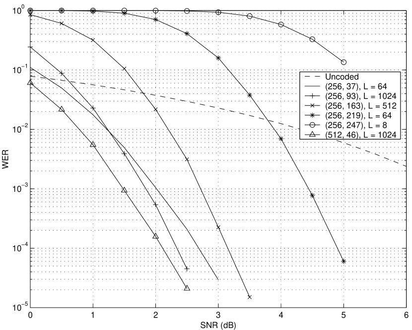
we summarize the results for all nontrivial RM codes of length 256 and for the code $\left\{\genfrac{}{}{0.0pt}{}{9}{2}\right\}$ of length 512. This figure presents almost exact experimental bounds on the error probability of ML decoding, along with the minimum lists $L$ that were used to meet ML-decoding performance. Here we also use permutation techniques to reduce this size $L.$ An interesting open problem is to provide a theoretical explanation as to why permutation decoding allows to substantially reduce the overall size $L$ of the lists over the basic recursive algorithms $\Psi_{r}^{m}$ and $\Phi_{r}^{m}$.

7 Conclusion

Our main conclusion is that recursive decoding of RM codes combines good performance and low complexity on moderate blocklengths up to 512. In turn, this allows us to partially fill the gap left by optimum maximum likelihood (ML) decoding and suboptimal iterative decoding. Note that the former has unfeasible complexity for nontrivial codes even on relatively short blocks of hundreds bits, while the latter becomes very efficient for turbo codes and low parity-check codes only on the blocks of thousands bits. An important open problem is whether recursive techniques can enable fast near-ML decoding for the lengths of 1024 and 2048. A positive solution to this problem would allow to completely fill the gap in the blocklengths left by the best algorithms known to date.

References

• [1] I.S. Reed, โ€œA class of multiple error correcting codes and the decoding scheme,โ€ IEEE Trans. Info. Theory, vol.ย IT-4, pp.ย 38โ€“49, 1954.
• [2] S.N. Litsyn, โ€œOn decoding complexity of low-rate Reed-Muller codes,โ€ Proc. 9thย All-Union Conf. on Coding Theory and Info. Transmission, Part 1, Odessa, USSR, pp.ย 202โ€“204, 1988 (in Russian).
• [3] G.A. Kabatyanskii, โ€œOn decoding of Reed-Muller codes in semicontinuous channels,โ€ Proc. 2ndย Int. Workshop โ€œAlgebr. and Comb. Coding Theoryโ€, Leningrad, USSR, 1990, pp.ย 87โ€“91 (in Russian).
• [4] F.J.ย MacWilliams, N.J.A.ย Sloane, The Theory of Error-Correcting Codes, North-Holland, Amsterdam, 1981.
• [5] R.E. Krichevskiy, โ€œOn the Number of Reed-Muller Code Correctable Errors,โ€ Dokl. Soviet Acad. Sciences, vol.ย 191, pp.ย 541โ€“547, 1970.
• [6] V. Sidelโ€™nikov and A. Pershakov, โ€œDecoding of Reed-Muller codes with a large number of errors,โ€ Probl. Info. Transmission, vol.ย 28, no. 3, pp.ย 80โ€“94, 1992.
• [7] G.D. Forney, โ€œCoset codes-part II: Binary lattices and related codes,โ€ IEEE Trans. Info. Theory, vol.ย 34, pp.ย 1152โ€“1187, 1987.
• [8] W. Feller, An Introduction to Probability Theory and its Applications. New York: Wiley, vol.ย 2, 1971.
• [9] Y.S. Han, C.R.P. Hartmann, and C.K. Mohan, โ€œEfficient heuristic search algorithms for soft-decision decoding of linear block codes,โ€ IEEE Trans. Inform. Theory, vol.ย 44, pp.ย 3023โ€“3038, 1998.
• [10] G. Schnabl and M. Bossert, โ€œSoft-decision decoding of Reed-Muller Codes as generalized multiple concatenated codes,โ€ IEEE Trans. Info. Theory, vol.ย 41, pp.ย 304โ€“308, 1995.
• [11] I. Dumer and R. Krichevskiy, โ€œSoft Decision Majority Decoding of Reed-Muller Codes,โ€ IEEE Trans. Info. Theory, vol.ย 46, pp.ย 258โ€“264, Jan.ย 2000.
• [12] I. Dumer, โ€œRecursive decoding of Reed-Muller codes,โ€ Proc. 37thย Allerton Conf. on Commun., Cont., and Comp., Monticello, IL, Sept.ย 22โ€“24, 1999, pp.ย 61โ€“69.