Quasars as standard candles I: The physical relation between disc and coronal emission

Abstract

Context. A tight non-linear relation exists between the X-ray and UV emission in quasars (i.e. $L_{\rm X}\propto L_{\rm UV}^{\gamma}$), with a dispersion of $\sim$0.2 dex over approximately three orders of magnitude in luminosity. Such observational evidence has two relevant consequences: (1) an ubiquitous physical mechanism must regulate the energy transfer from the accretion disc to the X-ray emitting corona, and (2) the non-linearity of the relation provides a new, powerful way to estimate the absolute luminosity, turning quasars into a new class of standard candles.

Aims. Here we propose a modified version of this relation, which involves the emission line full-width half maximum, $L_{\rm X}\propto L_{\rm UV}^{\hat{\gamma}}\upsilon_{\rm fwhm}^{\hat{\beta}}$.

Methods. We interpret this new relation through a simple, ad-hoc model of accretion disc corona, derived from previous works in the literature where it is assumed that reconnection and magnetic loops above the accretion disc can account for the production of the primary X-ray radiation.

Results. We find that the monochromatic optical-UV (2500 Å) and X–ray (2 keV) luminosities depend on the black hole mass and accretion rate as $L_{\rm UV}\propto M_{\rm BH}^{4/3}(\dot{M}/\dot{M}_{\rm Edd})^{2/3}$ and $L_{\rm X}\propto M_{\rm BH}^{19/21}(\dot{M}/\dot{M}_{\rm Edd})^{5/21}$, respectively. Assuming a broad line region size function of the disc luminosity $R_{\rm blr}\propto L_{\rm disc}^{0.5}$ we finally have that $L_{\rm X}\propto L_{\rm UV}^{4/7}\upsilon_{\rm fwhm}^{4/7}$. Such relation is remarkably consistent with the slopes and the normalisation obtained from a fit of a sample of 545 optically selected quasars from SDSS DR7 cross matched with the latest XMM–Newton catalogue 3XMM-DR6.

Conclusions. The homogeneous sample used here has a dispersion of 0.21 dex, which is much lower than previous works in the literature and suggests a tight physical relation between the accretion disc and the X-ray emitting corona. We also obtained a possible physical interpretation of the $L_{\rm X}-L_{\rm UV}$ relation (considering also the effect of $\upsilon_{\rm fwhm}$), which puts the determination of distances based on this relation on a sounder physical grounds. The proposed new relation does not evolve with time, and thus it can be employed as a cosmological indicator to robustly estimate cosmological parameters.

1 Introduction

Accreting super massive black holes (SMBHs) in the centre of galaxies (i.e. active galactic nuclei (AGN)) display characteristic observational features over a wide range of frequencies. Specifically, the AGN spectral energy distribution (SED) shows significant emission in the optical-UV, the so-called big blue bump (BBB), with a softening at higher energies (Sanders et al. 1989; Elvis et al. 1994; Richards et al. 2006; Trammell et al. 2007; Shang et al. 2011; Elvis et al. 2012). This emission is thought to origine from an optically thick disc surrounding the SMBH (Shakura & Sunyaev 1973; Novikov & Thorne 1973). The disc temperature goes from $\sim 5\times 10^{5}$K to $\sim 8.7\times 10^{4}$K for a SMBH of $10^{6}$ and $10^{9}M_{\odot}$ (at a given accretion) respectively, which corresponds to a peak emission in the range $\log\nu/{\rm Hz}\simeq 15-16.5$.

At X-ray energies ($k_{\rm B}T$$>$0.2–0.5 keV) the main continuum component is well described by a power law with spectral index $\alpha_{\rm X}\sim 1$ up to energies of a few hundred keV. The X-ray photons are produced by Compton up-scattering of disc UV photons by a hot electron plasma (the so-called X-ray corona). The energy loss through X-ray emission would cool down the electron plasma in a very short time scale if an efficient energy transfer mechanism from the disc to the corona were not in place. However, the physical nature of such a process is still poorly understood.

An important observational result concerning the link between the BBB (disc) and X-ray emission (corona) is provided by the non-linear correlation between the monochromatic optical luminosity at 2500 Å ($L_{\rm UV}$) and the one in the X–rays at 2 keV ($L_{\rm X}$, Tananbaum et al. 1979; Zamorani et al. 1981; Avni & Tananbaum 1986). The non-linear relationship between $L_{\rm X}$ and $L_{\rm UV}$ (parameterised as $\log L_{\rm X}=\gamma\log L_{\rm UV}+\beta$) has been found in both optically and X–ray selected AGN samples and exhibits a slope $\gamma$ around $0.5-0.7$ (Vignali et al. 2003; Strateva et al. 2005; Steffen et al. 2006; Just et al. 2007; Green et al. 2009; Lusso et al. 2010; Young et al. 2010; Marchese et al. 2012; Jin et al. 2012), implying that optically bright AGN emit relatively less X-rays than optically faint AGN. Such relation is independent of redshift, it is very tight ($\sim 0.2$ dex observed dispersion, Lusso & Risaliti 2016), and it has also been employed as a distance indicator to estimate cosmological parameters such as $\Omega_{\rm M}$ and $\Omega_{\Lambda}$. Thanks to the $L_{\rm X}-L_{\rm UV}$ relationship (or, more precisely, its version with fluxes), Risaliti & Lusso (2015) have built the first quasar Hubble diagram which extends up to $z\sim 6$, in excellent agreement with the analogous Hubble diagram for Type Ia supernovae in the common redshift range (i.e. $z\sim 0.01-1.4$). The observed $L_{\rm X}-L_{\rm UV}$ correlation (or its byproduct $\alpha_{\rm ox}-L_{\rm UV}$, where $\alpha_{\rm ox}=-0.384\log[L_{\rm X}/L_{\rm UV}]$) suggests that the disc-corona parameters are tightly linked and they must depend on the UV luminosity, and therefore ultimately on the black hole mass ($M_{\rm BH}$) and accretion rate ($\dot{M}$). Additionally, a positive correlation between the photon index and the accretion rate has been found in several previous analyses (e.g. Wang et al. 2004; Shemmer et al. 2006; Risaliti et al. 2009), which supports the idea that the coronal parameters are dependent on the accretion properties onto the SMBH. The major difficulty in interpreting such relations on physical grounds is that the origin of the X–ray emission in quasars is still a matter of debate.

Some attempts at interpreting the X–ray spectrum of quasars (in particular its slope, the photon index $\Gamma_{\rm X}$) were based on reprocessing of radiation from a non-thermal electron-positron pair cascade (Svensson 1982, 1984; Guilbert et al. 1983; Zdziarski et al. 1990). A highly energetic photon is absorbed in collision with an X–ray photon within the hot plasma producing an electron-positron pair, which in turn emits X-rays. This process is proportional to the source luminosity, inversely proportional to the source size, and, if the source is compact (a few tens of gravitational radii), it becomes an efficient cooling mechanism at $k_{\rm B}T<100$ keV that compensates for the additional heating (Dove et al. 1997). Recent results on the X-ray corona properties measured by NuSTAR have shown that pair production is an important process able to act as a thermostat in disc coronae (Fabian et al. 2015).

Another possibility is provided by a two-phase accretion disc model where the entire gravitational power is dissipated via buoyancy and reconnection of magnetic fields in a uniform hot plasma immediately above (and below) the cold opaque disc (Haardt & Maraschi 1991, 1993; Svensson & Zdziarski 1994; Di Matteo 1998). Soft X–ray photons from the disc are the main source of cooling of the hot electron within the plasma (phase 1), while the hard X-ray photons produced by the interaction via Compton scattering with the disc photons keep the X–ray corona at high temperatures (phase 2). When these two processes are balanced, a stable corona is formed. This model finds that, at a given disc temperature, the X–ray spectrum (approximated with a power-law) has a spectral index $\Gamma_{\rm X}\simeq 2$, originated from a fairly compact corona, in close agreement with observations. However, this model also predicts nearly equal optical-UV and X–ray luminosities, which is not consistent with observations. If the corona is not uniform but rather a clumpy medium, and only a fraction ($f$) of the accretion power is released in the hot phase, the resulting $L_{\rm UV}/L_{\rm X}$ ratio is higher than the value computed using a model with a more uniform corona (Haardt et al. 1994). Nonetheless, the number of active blobs necessary to match observations, and the value of $f$ are relatively arbitrary parameters.

The interaction between disc and corona has also been analysed in the viscosity-heated corona frame, where the heating in the corona is produced through friction as in the disc (Meyer et al. 2000; Liu et al. 2002a). However, this kind of model predicts an overly weak corona, hence an additional source of heating is required. The importance of magnetic field turbulence has been realised not only as a supplementary heating process in the formation of the corona itself (e.g. Galeev et al. 1979; Merloni & Fabian 2002; Liu et al. 2002b) but also as an efficient mean for the transport of the disc angular momentum (e.g. Balbus 2003). However, how the hot corona depends on $M_{\rm BH}$ and $\dot{M}$ still remains an open issue.

1.1 Outline of the work

In this paper we further analyse the $L_{\rm X}-L_{\rm UV}$ relation with the goal of understanding its physical origin. The works summarised above suggests two main conclusions. Firstly, a tight physical relation is present between the UV-emitting disk and the X-ray emitting corona. The intrinsic dispersion of this relation is rather small, approximately 0.18 dex or less over more than four orders of magnitude (Lusso & Risaliti 2016). Secondly, even though the physical connection between the accretion disc and the corona is still poorly understood, the amount of gravitational energy transferred from the disc to the corona most likely depends on the black hole mass, $M_{\rm BH}$, the accretion rate, $\dot{M}$, and the black hole spin which is in turn related to the accretion radiative efficiency, $\epsilon$. It is then straightforward to look for a physical relation connecting the X-ray luminosity with the parameters $M_{\rm BH}$ and $\dot{M}$ at a given value of $\epsilon$. If such a relation exists, than a correspondence between $L_{\rm X}$ and $L_{\rm UV}$ must be present, as $L_{\rm UV}$ also depends on $M_{\rm BH}$ and $\dot{M}$. We further notice that another observable relation among the same quantities is known: the virial relation between $L_{\rm UV}$, $M_{\rm BH}$, and the width of the broad emission lines in the optical-UV, $\upsilon_{\rm fwhm}$. Summarising, we have three relations linking the two physical parameters $M_{\rm BH}$ and $\dot{M}$ to three observable quantities: $L_{\rm UV}=f_{1}(M_{\rm BH},\dot{M})$, $L_{\rm X}=f_{2}(M_{\rm BH},\dot{M})$, $\upsilon_{\rm fwhm}=f_{3}(M_{\rm BH},\dot{M})$. Even without specifying the functions $f_{1}$, $f_{2}$, $f_{3}$, it is natural to expect that, by eliminating the parameters $M_{\rm BH}$ and $\dot{M}$, we can obtain a relation between $L_{\rm X}$, $L_{\rm UV}$, and $\upsilon_{\rm fwhm}$.

Based on these general motivations, our approach is based on two steps:

1. We will investigate the $L_{\rm X}(L_{\rm UV},\upsilon_{\rm fwhm})$ relation from an observational point of view, by analysing a sample of sources with reliable measurements of the X-ray and UV luminosity and the width of a broad emission line. We will restrict our analysis to a linear logarithmic relation, $\log L_{\rm X}=\gamma\log L_{\rm UV}+\beta\log\upsilon_{\rm fwhm}+K$.

2. We will discuss a possible simplified model, based on the Shakura-Sunyaev accretion disc, which, through an ad-hoc assumption on the way energy is transferred from the disc to the corona, is able to reproduce the observed relation, with an exact prediction of the two slopes $\gamma$ and $\beta$ and of the normalisation $K$.

Powerful radio-loud AGN represent approximately 10% of the total AGN population and show an enhanced X-ray emission linked to the jets with respect to the radio-quiet ones having similar optical luminosities (e.g. Zamorani et al. 1981; Wilkes & Elvis 1987; Cappi et al. 1997; Miller et al. 2011). Our toy model does not consider the extra complication linked to the jets, so we restrict our analysis to the radio-quiet AGN only.

Source luminosities are estimated by adopting a concordance flat $\Lambda$-cosmology with $H_{0}=70\,\rm{km\,s^{-1}\,Mpc^{-1}}$, $\Omega_{\mathrm{M}}=0.3$, and $\Omega_{\Lambda}=0.7$ (Komatsu et al. 2009).

2 The data

The broad-lined quasar sample we considered for our analysis has been built following a similar approach as the one described in Lusso & Risaliti (2016) (hereafter LR16). We started with the catalogue of quasar properties presented by Shen et al. (2011) (hereafter S11), which contains 105,783 spectroscopically confirmed broad-lined quasars. We removed from this catalogue all quasars flagged as broad absorption lines (BALs, i.e. sources with BAL_FLAG=0 are non-BALs) and radio-loud (i.e. having a radio loudness $R=F_{\nu,6\rm{cm}}/F_{\nu,2500\AA}\geq 10$, 8257 quasars, 8% of the main SDSS sample). This yields 91,732 SDSS quasars. We further excluded 136 quasars classified as BALs by Gibson et al. (2009). This pre-cleaned SDSS quasar sample (91,596 sources) is then cross-matched with the source catalogue 3XMM–DR6 (Rosen et al. 2016). 3XMM–DR6 is the third generation catalogue of serendipitous X-ray sources available online and contains 678,680 X–ray source detections (468,440 unique X-ray sources) made public on or before 2016 January 31. The net sky area covered (taking into account overlaps between observations) is $\sim$982 deg², for a net exposure time $\geq$1 ksec. For the matching we have adopted a maximum separation of 3 arcsec to provide optical classification and spectroscopic redshift for all objects. This yields 4,303 XMM observations : 2,725 unique sources, 739 of which have multiple ($\geq 2$) observations. To define a reasonably ‘clean’ sample we have applied the following quality cuts from the 3XMM–DR6 catalogue: SUM_FLAG$<$3 (low level of spurious detections), and HIGH_BACKGROUND$=$0 (low background levels). To further remove powerful radio loud quasars we made use of the catalogue published by Mingo et al. (2016), which is the largest available Mid-Infrared (WISE), X-ray (3XMM) and Radio (FIRST+NVSS) collection of AGN and star-forming galaxies: 2753 sources, 918 of which are considered radio-loud based on multiwavelength diagnostics (we refer to the paper for details). We excluded 17 quasars in our sample defined as radio loud in the MIXR catalogue within a matching radius of 2 arcsec. Since the MIXR catalogue has a prior on the W3 WISE magnitude, we may be missing a few more radio loud quasars due to that requirement. We thus cross-matched the FIRST/NVSS catalogue (2,129,340 objects) released by Mingo et al. (2016) with the 2,708 quasars using 30 arcsec matching radius. We estimated the 1.4 GHz luminosity from the combined FIRST/NVSS flux values. Quasars are then classified radio-loud if they have a 1.4 GHz luminosity higher than $5\times 10^{41}$ erg s^-1 (see Figures 15 and 16 by Mingo et al. 2016). The large majority of quasars with $L_{1.4\leavevmode\nobreak\ {\rm GHz}}>5\times 10^{41}$ erg s^-1 have an $R$ ratio higher than 10. We found 91 objects, 23 of which are radio-loud which have been further excluded from our sample. We have also excluded those objects without an estimate of the 2500Å flux, and the ones with a $\upsilon_{\rm fwhm}$ value for the Mg ii emission line lower than 2000 km s^-1 (we defer details for the latter requirement to § 2.1).

The remaining sample is composed of 3,386 XMM observations (2,119 unique quasars with both 0.5–2 and 2–12 keV fluxes, 592 of which with two or more observations). Following the results presented by LR16 (see their Section 4), we decided to average all observations for sources with multiple detections that meet our selection cuts. In this way, we reduce the effect of X–ray variability on the dispersion ($\sim 0.12$ dex, see § 4 in LR16).

The $L_{\rm UV}$ values are computed from the observed continuum flux densities at rest-frame 2500 Å ($F_{\rm UV}$) compiled by S11, which take into account the emission line contribution

The X–ray monochromatic luminosities and the $5\sigma$ minimum detectable flux at 2 keV ($F_{\rm min}$) are estimated following a similar approach to the one described by LR16 (we refer to their Section 2.1 for details). Specifically, the X-ray monochromatic luminosities are estimated from the soft 0.5-2 keV and 2-12 keV fluxes, $F_{S}$ and $F_{H}$, respectively, in the 3XMM-DR6 catalogue. These fluxes are computed assuming in each band a power law spectrum with photon index $\Gamma_{\rm X}$=1.7. We then used a single power law to fit $F_{S}$ and F_H simultaneously, obtaining a new value of the photon index, $\Gamma_{\rm X,1}$. Since the distribution of $\Gamma_{\rm X,1}$ is relatively broad (extending from $\sim 1$ to $\sim 3$ with an average of 1.9) and the effective area of the EPIC instruments has a strong energy dependence, a different photon index implies slightly different flux estimates in the two bands. We therefore apply a correction based on the average effective area as a function of energy, and estimate two corrected fluxes $F_{S,1}$, $F_{S,2}$. Then we repeat the power law fit and estimate a new photon index, $\Gamma_{\rm X,2}$. We iterate this procedure until we obtain a convergence ($\Delta\Gamma_{\rm X}<0.01$). The monochromatic flux at 2 keV (rest frame) is obtained from the final power law. For each detected object we have also computed the EPIC sensitivity ($5\sigma$ minimum detectable flux) at 2 keV using the same procedure as in LR16. Briefly, we have considered the pn, MOS1, and MOS2 on-time and off-axis values, where both MOS1 and MOS2 on-time and off-axis have been combined. The total MOS on-time and off-axis are the largest and smallest values of the two individual cameras, respectively. We then estimated the minimum detectable flux in the soft band corrected for vignetting. The sensitivity flux values at 2 keV ($F_{\rm min}$) are then calculated by assuming a photon index of 1.9 and finally combined by taking the sum of the pn and MOS fluxes in the case where both values are available.

The catalogue of SDSS-DR7 quasar properties published by S11 also contains a wealth of additional information that we considered in our analysis, such as, for example, black hole mass estimates, Eddington ratios, and $\upsilon_{\rm fwhm}$ for several lines, along with their uncertainties. We thus refer to S11 for details on how these parameters have been computed.

2.1 Selection of a ‘clean’ quasar sub-sample

Our aim is to select a sub-sample covering a redshift range as wide as possible, with precise estimates of $L_{\rm UV}$ and $L_{\rm X}$, by removing systematic effects and low-quality measurements. The possible sources of contamination/systematic error are: dust reddening in the optical-UV, gas absorption in X-rays, large statistical errors due to low X-ray flux, and Eddington bias due to the flux limit of the X-ray observations. Here we briefly discuss each of these points, and describe the filters we applied to obtain the final ‘best’ sample for our analysis.

1. Dust reddening. We used the SDSS photometry to compute, for each object, the slope $\Gamma_{1}$ of a $\log(\nu)-\log(\nu L\nu)$ power law in the rest frame 0.3–1 $\mu$m range, and the analogous slope $\Gamma_{2}$ in the 1450–3000 Å range. The wavelength coverage of the SDSS photometry does not cover the rest frame $1\mu m$ at $z\sim 2$, we thus considered the mid-infrared data from Spitzer and WISE, and the near-infrared data from the Two Micron All Sky Survey and UKIDSS published by Krawczyk et al. (2013) for the same SDSS-DR7 quasar sample. We selected all sources in the ($\Gamma_{1}$, $\Gamma_{2}$) plane within a circle centred at the reference values for a standard SED of quasars (see Risaliti & Lusso 2015 and LR16 for further details) with a radius corresponding to a reddening $E(B-V)\simeq 0.1$. Ninety-three percent of the sample (1965/2119) have $E(B-V)\leq 0.1$.

2. Signal-to-Noise. We selected only sources with a S/N$>$5 in the full 0.2–12 keV EPIC band. We did not apply an analogous filter on the optical spectra because we expect the error on the continuum flux measurement is always small compared with the uncertainties in the X-rays, for all the quasars in the spectroscopic SDSS samples. The fraction of objects excluded by such a signal-to-noise cut is 10%.

3. X-ray absorption. In order to avoid systematic underestimates of the the X-ray flux, we selected only sources with an X-ray photon index $\Gamma_{\rm X}>1.6$. Furthermore, we also excluded a few objects with $\Gamma_{\rm X}>3.0$. This filter is needed to avoid strong outliers (95% of our objects have $1.6<\Gamma_{\rm X}<2.8$) which may be due to observational issues such as incorrect background subtraction in one band, and/or low S/N.

4. Eddington bias. Due to X-ray variability, sources with an average X-ray flux close to the flux limit of the observation will be observed only in case of a positive flux fluctuation. This introduces an “Eddington bias” towards high fluxes. We therefore minimised this bias by including only sources whose minimum detectable flux is lower than the expected X-ray flux for each observation (we refer to Appendix A in LR16). On average, we have that the minimum detectable monochromatic flux at 2 keV is approximately $3\times 10^{-32}$ erg s^-1 cm^-2 Hz^-1. However, we caution that this value should not be considered the ‘survey limiting flux’ since the 3XMM–DR6 catalogue is not a proper flux-limited sample, but rather a collection of all XMM observations performed in a given period. It is thus not trivial to estimate the expected minimum flux for the whole data set. The effects of this bias can be reduced if no-detections are included in the statistical analysis. However, this would complicate the statistical analysis, and would make the estimate of the intrinsic dispersion of the correlations much more uncertain. LR16 showed that there is no significant variation on both slope and intercept (within their uncertainties) among censored and detected samples once the Eddington bias is minimised using the method discussed in their Appendix A. We therefore decided not to include censored data in our current work. We note that our procedure to minimise the Eddington bias is slightly circular: we need the $L_{\rm X}-L_{\rm UV}$ relation in order to estimate the ‘expected’ X-ray flux. We assumed that the expected slopes 0.6 with a variable normalisation. This filter is applied iteratively in a similar way as discussed in LR16. We obtained a perfect convergence (i.e. no more sources rejected) after just one iteration.

5. Homogeneous line properties. In order to explore the dependence among $L_{\rm X}$, $L_{\rm UV}$, and $\upsilon_{\rm fwhm}$, we selected only sources with an observation of the Mg ii $\lambda$2800 Å full-width half maximum higher than 2000 km s^-1. This filter ensures homogeneity in the estimate of the line parameters, and, given the redshift distribution of our sample, rejects only 20% of the sample which lies outside the range where Mg ii is observed ($z<0.35$ and $z>2.3$), and 5% of the sample with $\upsilon_{\rm fwhm}<2000$ km s^-1 within that redshift range. This provides the widest redshift coverage possible given the SDSS spectral coverage. Other emission lines as, for example, H $\beta$ and C iv would bias the sample towards low/high redshift quasars, thus are less suitable for cosmological studies. It is also well known that the C iv line may be affected by non-gravitational motions (e.g. outflows), and therefore the interpretation for that line is likely to be non trivial.

While all the points discussed above have a clear qualitative justification, it is not obvious how to choose the numerical parameters of each filter based on general considerations. Here we apply a very conservative empirical criterion: if the effects discussed above introduce a bias in the estimates of the X-ray and UV fluxes, we will observe a change in the $L_{\rm X}-L_{\rm UV}-\upsilon_{\rm fwhm}$ relation when we start applying a given filter. There will be a range in the filter parameters where if we tighten the filter, the bias is reduced, and the measured relation changes. When the bias is completely removed, if we further tighten the filter, we will not see any further change in the relation, but only a decrease in the number of selected sources. The parameters described above are all significantly beyond these threshold values: in other words, if we relax some of them (for example, allowing for more reddened objects, or accepting sources with $\Gamma_{\rm X}>1.5$, or changing the threshold for the Eddington bias from 2 $\sigma$ to 1.5 $\sigma$) this has no effect on the results of the analysis of the $L_{\rm X}-L_{\rm UV}-\upsilon_{\rm fwhm}$ relation.

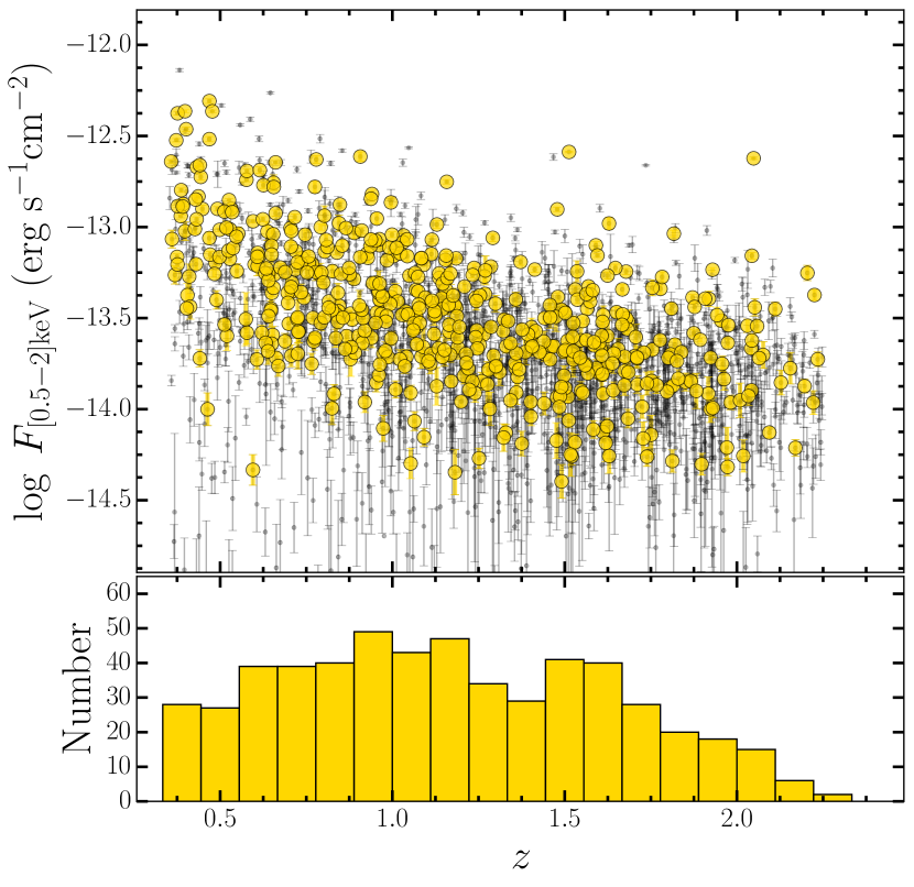
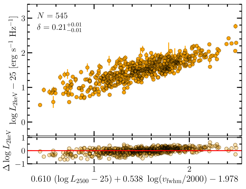
The final “best” sample consists of 545 sources and is shown in Figure 1, spanning a redshift range of 0.358–2.234. This is only $\sim$25% of the initial sample. As mentioned above, we could relax the filtering criteria and add a few hundred more objects, but at the price of less precise measurements and possible residual small systematic effects. Since our aim is to analyse a three-parameter linear correlation, we believe our sample is large enough for our purpose, and we prefer to favour sample cleanness over higher statistics. This choice is supported by the results of the analysis, which are discussed in detail in Section 3: the errors on the parameters of the $L_{\rm X}-L_{\rm UV}-\upsilon_{\rm fwhm}$ correlation are relatively small; relaxing the parameters and adding more sources (still in the bias-free range) means we obtain a larger intrinsic dispersion (due to the lower quality measurements included in the sample) and the final uncertainties on the best fit parameters do not decrease significantly.

Figure 1: Top panel: Distribution of the observed $0.5-2$keV flux versus redshift for the main sample of 2,119 quasars (small black points) and the one of 545 sources (gold points). Bottom panel: Redshift distribution for the best quasar sample.

Figure 2: The $L_{\rm X}-L_{\rm UV}-\upsilon_{\rm fwhm}$ plane seen edge-on. Both optical and X-ray luminosities have been normalised to $10^{25}$ erg s^-1 Hz^-1. The $\upsilon_{\rm fwhm}$ values are taken from S11 and are normalised to 2000 km s^-1. Here we considered the $\upsilon_{\rm fwhm}$ estimated from the whole Mg ii emission line. The bottom panel shows the residuals defined as the difference between the observed monochromatic X-ray luminosity at 2 keV and the best fitting function.

3 Statistical analysis

To fit the data in the three-dimensional plane defined as $\log L_{\rm X}=\hat{\gamma}\log L_{\rm UV}+\hat{\beta}\log\upsilon_{\rm fwhm}+\hat{K}$, we adopted the Python package emcee (Foreman-Mackey et al. 2013), which is a pure-Python implementation of Goodman & Weare’s affine invariant Markov chain Monte Carlo (MCMC) ensemble sampler. We accounted for the dependent variable $Z$ against the independent variables $X$ and $Y$ (i.e. $Z=\hat{\gamma}X+\hat{\beta}Y+\hat{K}$), and we included uncertainties on both $L_{\rm X}$ and $\upsilon_{\rm fwhm}$. Since uncertainties on $L_{\rm UV}$ are not provided in the SDSS quasar catalogue, we assumed a 2% uncertainty on the continuum flux measurement, which is roughly the average uncertainty on the bolometric luminosity values in the SDSS quasar catalogue. None of the results presented significantly depend on our assumed uncertainty on the optical data. Slope and intercept estimated assuming 2% optical uncertainty are consistent within 1.5$\sigma$ with the fits performed with 5% and 10% uncertainty on $L_{\rm UV}$, and a normal distribution of uncertainties on $L_{\rm UV}$ having a mean at $\sim$0.25 dex ($\sim 30$%). We then fitted $\hat{\gamma}$, $\hat{\beta}$, $\hat{K}$, and the intrinsic dispersion of the relation $\delta$. We normalised $L_{\rm UV}$ and $L_{\rm X}$ to $10^{25}$ erg s^-1 Hz^-1, while $\upsilon_{\rm fwhm}$ has been normalised to 2000 km s^-1. Here we considered the $\upsilon_{\rm fwhm}$ values obtained from the whole Mg ii emission line. Rafiee & Hall (2011) found that their Mg ii line dispersion estimates are rather different from those of Shen et al. (2008). Specifically, they found that using $\upsilon_{\rm fwhm}$ as a line width indicator may overestimate the $M_{\rm BH}$ values for the broadest emission lines, and underestimate $M_{\rm BH}$ for the narrowest emission lines as compared with $M_{\rm BH}$ computed using the line dispersion. This may introduce a tilt of the plane in the $\upsilon_{\rm fwhm}$ direction. Even though we believe that the $\upsilon_{\rm fwhm}$ estimates provided by S11 are more robust than those published in their previous analysis. Without other measurements for a statistically significant sample of quasars to compare with, we cannot explore this point any further.

Figure 3: Rest-frame monochromatic luminosities $\log L_{\rm X}$ against $\log L_{\rm UV}$ for the final “best” sample of 545 quasars (orange circles) as described in § 2.1. The results from the emcee regression (black solid line) are also reported. Red thin lines represent 100 different realisations of the $L_{\rm UV}-L_{\rm X}$ relation. The lower panel shows the residuals of $\log L_{\rm X}$ and $\log L_{\rm UV}$ with respect to the emcee best-fit line.

Table 1: Results of the regression analysis of the $L_{\rm X}-L_{\rm UV}-\upsilon_{\rm fwhm}$ plane parametrised as $\log L_{\rm X}=\hat{\gamma}\log L_{\rm UV}+\hat{\beta}\log\upsilon_{\rm fwhm}+\hat{K}$.

Sample	$\hat{\gamma}$	$\hat{\beta}$	$\hat{K}$	$\delta$	$N_{\rm tot}$
Main	0.564$\pm$0.014	0.379$\pm$0.046	-1.725$\pm$0.076	0.32$\pm$0.01	2119(592)
E(B–V)$\leq$0.1	0.562$\pm$0.015	0.404$\pm$0.048	-1.722$\pm$0.083	0.31$\pm$0.01	1965(551)
E(B–V)$\leq$0.1 – S/N$>$5	0.556$\pm$0.015	0.389$\pm$0.048	-1.662$\pm$0.082	0.30$\pm$0.01	1758(459)
E(B–V)$\leq$0.1 – S/N$>$5 – $1.6\leq\Gamma_{\rm X}\leq 2.8$	0.559$\pm$0.014	0.499$\pm$0.048	-1.660$\pm$0.076	0.24$\pm$0.01	1345(292)
E(B–V)$\leq$0.1 – S/N$>$5 – $1.9\leq\Gamma_{\rm X}\leq 2.8$	0.579$\pm$0.015	0.552$\pm$0.053	-1.789$\pm$0.084	0.22$\pm$0.01	929(179)
E(B–V)$\leq$0.1 – S/N$>$5 – $1.9\leq\Gamma_{\rm X}\leq 2.8$ – EB	0.610$\pm$0.019	0.538$\pm$0.072	-1.978$\pm$0.100	0.21$\pm$0.01	545(105)

To check if our results depend on the regression technique, we also considered the LINMIX_ERR method (Kelly 2007), which takes account of measurement uncertainties on both independent and dependent variables, non-detections (not considered in the following analysis), and intrinsic scatter by adopting a Bayesian approach to compute the posterior probability distribution of parameters, given the observed data. In general, the resulting fitting parameters output of LINMIX_ERR are fully consistent within the uncertainties of those of emcee, thus we decided to report the parameter values from emcee only.

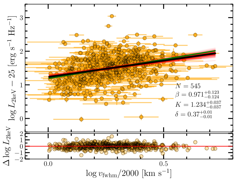
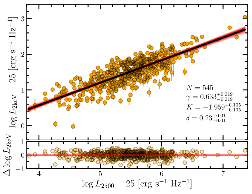
Figure 2 shows an edge-on view of the $L_{\rm X}-L_{\rm UV}-\upsilon_{\rm fwhm}$ plane. The best-fit regression equation is

$$(\log L_{\rm X}-25)=(0.610\pm 0.019)(\log L_{\rm UV}-25)+$$

$$(0.538\pm 0.072)[\log\upsilon_{\rm fwhm}-(3+\log 2)]+(-1.978\pm 0.100),$$ (1)

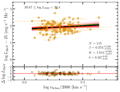
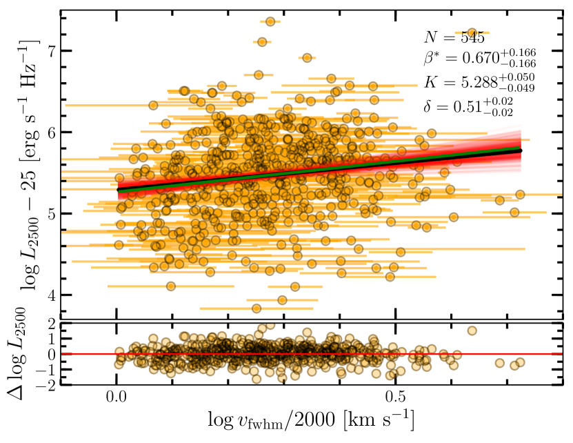
with a dispersion of $\sim$0.21 dex, which is an extremely tight correlation (with a Pearson $R$ coefficient of 0.83)The Student’s t-test for $\hat{\gamma}$ and $\hat{\beta}$ yields a significance that these slopes are different from zero of approximately $32$ and $7\sigma$, respectively. We have also evaluated how slopes and dispersion change as a function of various selection cuts. The summary of our findings is provided in Table 1. Interestingly, both slopes are roughly consistent within the 2$\sigma$ level irrespective of the selection cut, yet the dispersion decreases as the cuts become more conservative on the quality of the data. A more in-depth analysis of the dispersion and of how it depends on X–ray variability, disc inclination, and so on is the subject of a forthcoming paper. Figure 3 shows the $L_{\rm X}-L_{\rm UV}$ relation without the dependence on $\upsilon_{\rm fwhm}$ ($R=0.81$), with $\gamma$ statistically different from zero at $\sim 32\sigma$. Both slope and normalisation are in agreement with previous works in the literature on optically selected samples (e.g. Strateva et al. 2005; Steffen et al. 2006; LR16). These findings are not altered if we repeat the analysis by doubling the uncertainties on $L_{\rm X}$. The Fisher’s F-test for the additional dependence of the $L_{\rm X}-L_{\rm UV}$ relation on $\upsilon_{\rm fwhm}$ yields $F=28$ with a $p-$value of $2.7\times 10^{-12}$ that the dependence on $\upsilon_{\rm fwhm}$ is not significant. We must notice that the residuals ($\Delta\log L_{\rm X}$, defined as the difference between the observed monochromatic X-ray luminosity at 2 keV and the best fitting function) plotted in Figure 2 are slightly tilted, meaning that the best fit under/overestimate s the slope at low/high values of $L_{\rm UV}$ and $\upsilon_{\rm fwhm}$. To investigate this, further we evaluated how slopes and dispersion in the $L_{\rm X}-L_{\rm UV}-\upsilon_{\rm fwhm}$ plane change by slicing the $L_{\rm X}-L_{\rm UV}$ and the $L_{\rm X}-\upsilon_{\rm fwhm}$ relationships as a function of $\upsilon_{\rm fwhm}$ and $L_{\rm UV}$, respectively. Details are provided in Appendix A. Summarising, we found that the additional dependence of the observed $L_{\rm X}-L_{\rm UV}$ correlation on $\upsilon_{\rm fwhm}$ is statistically significant and may point towards a much tighter connection between accretion disc physics and X-ray corona than has been found previously.

3.1 Redshift dependence

Figure 4: Evolution of the $\hat{\gamma}$ and $\hat{\beta}$ parameters with redshift. Orange points (along with their uncertainties) are the results of the fitting procedure of the function $\log F_{\rm X}=\hat{\gamma}_{z}\log F_{\rm UV}+\hat{\beta}_{z}\upsilon_{\rm fwhm}+\hat{K}$ in narrow redshift bins (see § 3.1 for details). The red solid line represents the predicted value of $4/7$ (§ 4). The blue solid line and shaded area represent the $\hat{\gamma}$ and $\hat{\beta}$ from the global fit using luminosities as discussed in § 3. The grey solid and dashed lines are the weighted means with uncertainties of the orange points.

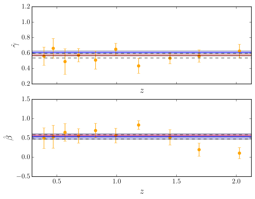
We now discuss the redshift evolution $L_{\rm X}-L_{\rm UV}-\upsilon_{\rm fwhm}$ relation where fluxes are considered instead of luminosities. To do so, we analysed the best quasar sample only as this will be the one used to compute the cosmological parameters in Paper II. We divided our sample into equally spaced redshift bins in $\log z$ with a $\Delta\log z<0.1$ to minimise the scatter due to the different luminosity distances compared to the intrinsic dispersion within each bin. We also require sufficiently populated bins (i.e. $N\geq 20$ objects) for a statistically meaningful fit. We split the sample into ten intervals with $\Delta\log z=0.08$ and, for each redshift interval, we performed a fit of the $F_{\rm X}-F_{\rm UV}-\upsilon_{\rm fwhm}$ relation, $\log F_{\rm X}=\hat{\gamma}_{z}\log F_{\rm UV}+\hat{\beta}_{z}\upsilon_{\rm fwhm}+\hat{K}$, with free $\hat{\gamma}_{z}$ and $\hat{\beta}_{z}$. The results for the best-fit slopes $\hat{\gamma}_{z}$ and $\hat{\beta}_{z}$ as a function redshift are shown in Figure 4. Both $\hat{\gamma}_{z}$ and $\hat{\beta}_{z}$ slopes are consistent with a constant value at all redshifts, without any significant evolution with time, and best-fit weighted mean values of $\hat{\gamma}_{z}\simeq 0.566\pm 0.030$ and $\hat{\beta}_{z}\simeq 0.529\pm 0.056$.

4 Toy model

In this section we outline a simple, ad-hoc physical model which provides the relationships between the disc and the X-ray emission in terms of the black hole mass, the accretion rate, and the distance to the black hole ($R$). Our main goal is to link such relations with observable quantities, thus delivering a correlation that can be easily compared with the results of our statistical analysis. In our modelisation, we introduce the following non-dimensional parameters:

$$m=\frac{M_{\rm BH}}{M_{\odot}},\quad r=\frac{R}{R_{\rm S}}=\frac{R}{3\times 10^{5}{\rm cm}}m^{-1},$$

$$\dot{m}=\frac{\dot{M}}{\dot{M}_{\rm Edd}}\simeq\frac{\dot{M}}{10^{18}{\rm gr\leavevmode\nobreak\ s^{-1}}}m^{-1},$$ (2)

where $R_{\rm S}=2GM_{\rm BH}/c^{2}$ is the Schwarzschild radius, $\dot{M}_{\rm Edd}$ is the Eddington accretion

$$\dot{M}_{\rm Edd}=\frac{\epsilon L_{\rm Edd}}{c^{2}},$$ (3)

and $L_{\rm Edd}=\frac{4\pi cGM_{\rm BH}\mu m_{\rm p}}{\sigma_{\rm T}}$ defines the Eddington luminosity: $\sigma_{\rm T}$ is the Thomson cross section, $\mu$ is the mean atomic weight, which we assumed to be equal to 0.615 throughout the paper (approximate for a fully ionised cosmic mixture), and $\epsilon$ is the radiative efficiency assumed to be 1/12 (appropriate for a steady SMBH).

To compare the results with observations, we need to have a relation that transforms our physical variables $m$ and $\dot{m}$ to the observable ones. The parameter $m$ is usually obtained from the virial relationship (Peterson 2014, and references therein)

$$m=\frac{R_{\rm blr}\upsilon_{\rm fwhm}^{2}}{GM_{\odot}},$$ (4)

where $\upsilon_{\rm fwhm}$ is the full width at half maximum of the line, $R_{\rm blr}$ represents the size of the broad line region, and a virial coefficient factor, which accounts for our ignorance of the broad line region geometry, of the order of unity (McLure & Dunlop 2004). The parameter $R_{\rm blr}$ is proportional to the square root of the quasar bolometric luminosity ($L_{\rm bol}$), $R_{\rm blr}=kL_{\rm bol}^{0.5}$ (Trippe 2015), and $\kappa$ is a calibration constant. From equation (4) we have that

$$m\simeq 7.5\times 10^{-27}\kappa L_{\rm bol}^{0.5}\upsilon_{\rm fwhm}^{2}\simeq 3\times 10^{13}\kappa L_{\rm bol,46}^{0.5}\upsilon_{\rm{fwhm},2000}^{2},$$ (5)

where $L_{\rm bol,46}$ and $\upsilon_{\rm{fwhm},2000}$ are normalised to $10^{46}$ erg s^-1 and 2000 km s^-1, respectively.

4.1 The predicted monochromatic luminosity at 2500 Å

The most widely used model of accretion disc physics is provided by the disc structure equations published by Shakura & Sunyaev (1973) (hereafter SS73), which assume hydrostatic equilibrium in the vertical direction, conservation of angular momentum (the torque vanishes at the inner stable circular orbit), and disc energy balance. The exchange of angular momentum along the disc is provided by viscous stresses within the fluid, through an ad-hoc effective viscosity, and making use of standard hydrodynamics without the inclusion of magnetic fields. This approach has been very effective especially in simulations, since the full magnetohydrodynamic treatment can be numerically costly. For these reasons, the SS73 parametrisation still finds wide application today (see Abramowicz & Fragile 2013 for a detailed discussion. On the other hand, from an observational perspective, the SS73 model has been challenged, especially in reproducing the shape of the SED near the ultraviolet peak (Lawrence 2012) through the soft X-ray region (e.g. Blaes & Socrates 2001). Moreover, it does not provide an explanation for the X–ray emission observed in quasars at energies higher than 0.5 keV. In what follows, we considered an approach similar to that in Merloni (2003). We summarise below the basic assumptions and equations that we use throughout the paper.

The total disc luminosity ($L_{\rm disc}$) of a Keplerian geometrically thin, optically thick, accretion disc is obtained from the integral of the viscous dissipation rate (e.g. Pringle 1981; Field & Rogers 1993), at a given $R$, within the disc defined as

$$D(R)=\frac{3GM\dot{M}}{4\pi R^{3}}\left[1-\left(\frac{R_{0}}{R}\right)^{1/2}\right],$$ (6)

where $\left[1-\left(\frac{R_{0}}{R}\right)^{1/2}\right]$ is a dimensionless factor set by the inner boundary condition at the radius $R_{0}$. When written as above, this factor does not include relativistic effects (Novikov & Thorne 1973), which are important but not dominant (we refer to equations 3–5 and table 1 in Laor & Davis 2011, and Riffert & Herold 1995; Merloni & Fabian 2003 for a detailed discussion). In what follows we thus assume a Newtonian regime. From equation (6) the expression of $L_{\rm disc}$ at $R_{0}=3R_{\rm S}$ (i.e. the innermost stable circular orbit of a non-rotating SMBH) is

$$L_{\rm disc}=\frac{GM\dot{M}}{6R_{\rm S}}=\frac{\dot{M}c^{2}}{12}\simeq 7.7\times 10^{37}\leavevmode\nobreak\ m\leavevmode\nobreak\ \dot{m}\quad{\rm erg\leavevmode\nobreak\ s^{-1}}.$$ (7)

If each element of the disc radiates as a black body, the disc temperature is given by equating the black body flux to the dissipation rate. The disc temperature at a given distance can be written as

$$T_{\rm disc}(r)=T_{0}\leavevmode\nobreak\ r^{-3/4}J(r)^{1/4},$$ (8)

where $J(r)=(1-\sqrt{3/r})$ and $T_{0}=(3GM\dot{M}/8\pi\sigma_{\rm B}R_{\rm S}^{3})^{1/4}$. We assume for simplicity that there are no additional dissipative mechanisms within the disc, which will produce soft photons that will interact with those in the plasma, lowering the temperature through the Compton cooling mechanism.

By assuming that $L_{\nu}\propto\nu^{-\gamma_{\rm o}}$ we can now estimate the monochromatic optical luminosity at 2500 Å as

$$L_{\rm UV}=\frac{L_{\rm disc}\leavevmode\nobreak\ (1-\gamma_{\rm o})}{\nu_{\rm o}}\left(\frac{\nu_{\rm o}}{\nu_{\rm c}}\right)^{1-\gamma_{\rm o}},$$ (9)

where $\nu_{\rm c}$ is the characteristic frequency of the disc, and $\nu_{\rm o}$ is the reference optical frequency. The peak frequency of the big blue bump is

$$\nu_{\rm c}\simeq 2.8\frac{k_{\rm B}}{h}T_{\rm disc}(r_{\rm max})\simeq 7.2\times 10^{17}m^{-1/4}\leavevmode\nobreak\ \dot{m}^{1/4}\quad\rm Hz,$$ (10)

where $T_{\rm disc}(r_{\rm max})$ is defined at the radius where the maximum in the disc temperature occurs (i.e. $r_{\rm max}=49/12$, thus $T_{\rm disc}(r_{\rm max})\simeq 0.21T_{0}\simeq 1.2\times 10^{7}m^{-1/4}\leavevmode\nobreak\ \dot{m}^{1/4}$). The final expression for $L_{\rm UV}$ is

$$L_{\rm UV}\simeq\frac{7.7\times 10^{37}\leavevmode\nobreak\ (1-\gamma_{\rm o})}{\nu_{\rm o}^{\gamma_{\rm o}}}\left(7.2\times 10^{17}\right)^{(\gamma_{\rm o}-1)}\times$$

$$m^{(5-\gamma_{\rm o})/4}\leavevmode\nobreak\ \dot{m}^{(3+\gamma_{\rm o})/4},$$ (11)

in erg s^-1 Hz^-1. For a SS73 disc, the optical-ultraviolet spectrum has $\gamma_{\rm o}=-1/3$, which has been proved to be consistent through observations of the polarised light interior to the dust-emitting region in several low-redshift quasars (Kishimoto et al. 2008). We finally have that

$$L_{\rm UV}\simeq 1.7\times 10^{19}m^{4/3}\leavevmode\nobreak\ \dot{m}^{2/3}$ erg s$^{-1}$ Hz$^{-1},$$ (12)

which expresses the dependence of $L_{\rm UV}$ on the physical parameters $m$ and $\dot{m}$.

4.2 The predicted monochromatic luminosity at 2 keV

Our formalism is mainly based on the one in Svensson & Zdziarski (1994) (SZ94 hereinafter). They discussed the physical conditions of the disc-corona system under the assumption that the cold accretion disc is geometrically thin (i.e. SS73). In their model, a fraction ($f$) of the accretion power associated with the transport of angular momentum stored in the disc (via magnetic field loops, and/or flux tubes, for instance) is dissipated (only once the accretion power reaches the disc surface) in a hot corona through an unspecified physical dissipation mechanism. The accretion rate in the disc is thus $(1-f)$ of the total accretion. SZ94 found that for $f\simeq 1,$ the emission from a hot corona becomes relevant only when the gas pressure dominates over radiation inside the disc. The radius ($r_{\rm tr}$) defining the boundary between the radiation dominated region and the gas pressure dominated zone (i.e. the outer/inner boundary of the radiation/gas pressure dominated zone) can be computed by assuming that the radiation pressure equates the gas pressure, and thus

$$r_{\rm tr}\simeq 120\left(\alpha m\right)^{2/21}\dot{m}^{16/21}(1-f)^{6/7}J(r)^{16/21},$$ (13)

in units of $R_{\rm S}$, where $\alpha$ is the standard disc viscosity parameter. We note that equation (13) assumes a radiative diffusion of the order of unity (i.e. SS73), and a normalisation factor that differs from equation (29) in SZ94, as the latter has been estimated for $\epsilon=1$ and $\mu=1$. Additionally, the $rJ(r)^{-16/21}$ factor has a minimum at $\tilde{r}=5.72$, which corresponds to a critical accretion rate of the order of 1%. For $\dot{m}$ lower than the critical one, the factor $120\left(\alpha m\right)^{2/21}\dot{m}^{16/21}(1-f)^{6/7}$ is always smaller than $rJ(r)^{-16/21}$ and there are no solutions (see SZ79 and Merloni & Fabian 2002 for additional discussion). Therefore, our toy model is valid only for accretion rates higher than the critical one. To estimate the X–ray coronal emission we assume that the hot corona is powered by a magnetised flux emerging (in a dissipationless fashion) from the disc to balance the amplifying effects of the magneto-rotational instability (MRI), which produces turbulence able to transport angular momentum in the disc itself. A detailed discussion of this phenomenon is presented by Merloni & Fabian (2002) (hereafter MF02, see their Section 2 and references therein). MRI works at full efficiency in cases where the disc is gas-pressure dominated. When the disc is radiation-pressure dominated, the MRI is quenched and the (much lower) value of the emerging disc flux becomes, to a certain extent, model-dependent. We assume a sharp transition at the radius $r_{\rm tr}$ where the gas and radiation pressures are equal. In the gas dominated zone, the total power released locally by the accretion is divided equally between the power radiated by the disc itself and that transferred to the corona. On the other side (i.e. the radiation dominated zone), all the power is radiated within the disc and the amount of energy transferred to the corona is negligible. Therefore, given our assumptions, we have that

$$L_{\rm cor}\simeq 2\times 10^{36}\alpha^{-2/21}m^{19/21}\dot{m}^{5/21}(1-f)^{-6/7}J(r)^{-16/21}\quad{\rm erg\leavevmode\nobreak\ s^{-1}}.$$ (14)

The monochromatic X–ray luminosity at 2 keV can be written as

$$L_{\rm X}=L_{\rm cor}(1-\alpha_{\rm X})\frac{\nu_{\rm X}^{-\alpha_{\rm X}}}{\nu_{2}^{1-\alpha_{\rm X}}-\nu_{1}^{1-\alpha_{\rm X}}},$$ (15)

where $\alpha_{\rm X}$ represents the slope of the X–ray SED (related to the X–ray photon index as $\alpha_{\rm X}=\Gamma_{\rm X}-1$). We considered an energy range between 0.1 keV and 40 keV, which has a mean geometric energy of 2 keV (i.e. $\sqrt{0.1\times 40}\simeq 2$ keV). By substituting equation (14) into the above equation, and assuming a $\alpha_{\rm X}=0.9$ (Young et al. 2009, 2010), we finally have

$$L_{\rm X}\simeq 6.6\times 10^{17}\leavevmode\nobreak\ \alpha^{-2/21}m^{19/21}\dot{m}^{5/21}\leavevmode\nobreak\ (1-f)^{-6/7}\leavevmode\nobreak\ J(r)^{-16/21}\leavevmode\nobreak\ \quad{\rm erg\leavevmode\nobreak\ s^{-1}}.$$ (16)

4.3 The predicted relation between X–ray and optical luminosity of quasars

The physical relation between $L_{\rm X}$ and $L_{\rm UV}$ can be calculated by solving the system of equations (5), (12), and (16). Provided that $L_{\rm bol}$ is given by equation (7), we can write equation (5) as

$$m\simeq 4.3\times 10^{-15}\kappa^{2}\leavevmode\nobreak\ \dot{m}\leavevmode\nobreak\ \upsilon_{\rm fwhm}^{4}.$$ (17)

It follows that

$$L_{\rm X}\simeq 6.6\times 10^{4}\dot{m}^{24/21}\alpha^{-2/21}(1-f)^{-6/7}J(r)^{-16/21}\kappa^{38/21}\upsilon_{\rm fwhm}^{76/21}$$ (18)

and

$$L_{\rm UV}\simeq 1.2\leavevmode\nobreak\ \dot{m}^{2}\kappa^{8/3}\upsilon_{\rm fwhm}^{16/3}$$ (19)

in erg s^-1. From the two equations above we finally have

$$L_{\rm X}\simeq 6\times 10^{4}\leavevmode\nobreak\ L_{\rm UV}^{4/7}\leavevmode\nobreak\ \upsilon_{\rm fwhm}^{4/7}\leavevmode\nobreak\ \alpha^{-2/21}\kappa^{2/7}\times$$

$$(1-f)^{-6/7}J(r)^{-16/21}\leavevmode\nobreak\ {\rm erg\leavevmode\nobreak\ s^{-1}}.$$ (20)

To compare the relation above with the results of our regression analysis, we must normalise both $L_{\rm X}$ and $L_{\rm UV}$ to $10^{25}$ erg s^-1 Hz^-1 and $\upsilon_{\rm fwhm}$ to 2000 km s^-1, thus equation (4.3) becomes

$$L_{{\rm X},25}\simeq\leavevmode\nobreak\ 0.06\leavevmode\nobreak\ L_{{\rm UV},25}^{4/7}\leavevmode\nobreak\ \upsilon_{{\rm fwhm},2000}^{4/7}\leavevmode\nobreak\ \alpha^{-2/21}\kappa^{2/7}(1-f)^{-6/7}J(r)^{-16/21}.$$ (21)

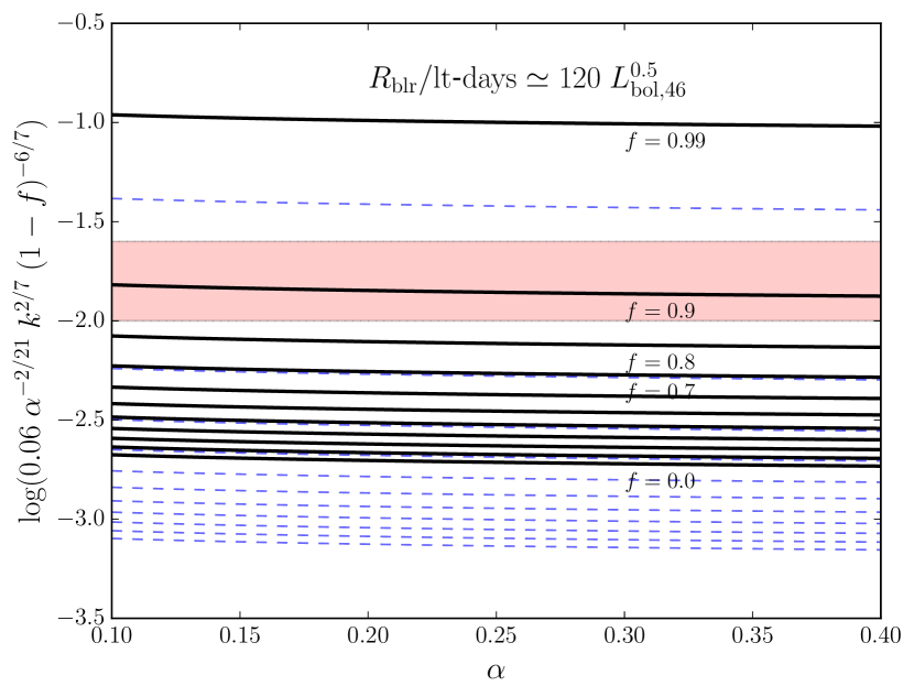
We note that the additional correction due to the factor $J(r)^{-16/21}$ of equation (4.3) makes the slopes from $\hat{\gamma}=\hat{\beta}=0.571$ to $\hat{\gamma}\simeq 0.581$ and $\hat{\beta}\simeq 0.531$, still in agreement with our findings. Figure 5 shows how the normalisation of equation (21) changes as a function of $\alpha$, $\kappa$, and $f$. We fixed the $\kappa$ factor to $3\times 10^{-6}$, which corresponds to a broad line region size of approximately $3\times 10^{17}$ cm ($\sim 120$ light days, or $\sim$0.1 parsec) for a bolometric luminosity of $10^{46}$ erg s^-1, typical of quasars (e.g. Kaspi et al. 2005). The $\alpha$ parameter varies in the range 0.1–0.4 (King et al. 2007), while $f$ goes from 0 to 0.99. The normalisation of the relation presents a large scatter, which can be a factor of $\sim 2$ in logarithm (i.e. orders of magnitude) depending on the value of $f$ (see also Fig. 1 in Merloni 2003). Despite our crude assumptions, not only are the observed slopes of the $L_{\rm X}-L_{\rm UV}-\upsilon_{\rm fwhm}$ relation in really good agreement with the ones of equation (21), but also the observed normalisation is in a range consistent with the predictions.

Figure 5: The logarithm of the normalisation of equation (21) as a function of $\alpha$. The $\kappa$ factor has been fixed to $3\times 10^{-6}$, corresponding to a broad line region size of approximately $3\times 10^{17}$ cm ($\sim 120$ light days) for a bolometric luminosity of $10^{46}$ erg s^-1. The solid black lines correspond to different values of $f$, which go from 0 to 0.99 from bottom to top. The dashed blue lines correspond to the normalisation at $\sim$4 light days in the same range of $f$. The red shaded area indicates the range of observed $\hat{K}$ (see table 1).

We have also investigated how the slopes vary if we take $\gamma_{\rm o}$ as a free parameter. Equation (4.3) becomes

$$L_{\rm X}\propto L_{\rm UV}^{4/7}\upsilon_{\rm fwhm}^{(16+12\gamma_{\rm o})/12},$$ (22)

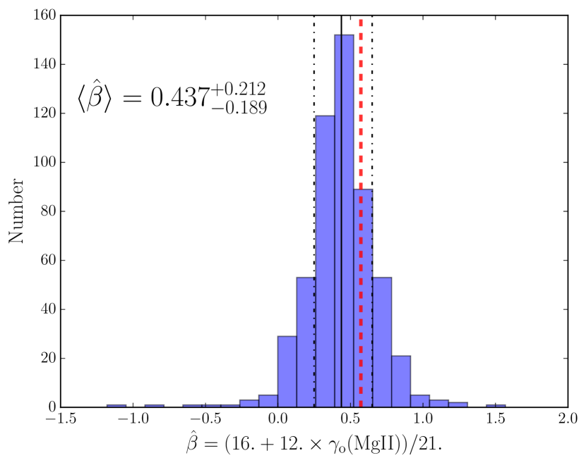
thus $\hat{\gamma}$ does not have any dependence on $\gamma_{\rm o}$. By considering the continuum spectral slopes estimated by S11 for the Mg ii emission line, we can explore how $\hat{\beta}$ varies as a function of $\gamma_{\rm o}$. Such slopes are estimated by taking the continuum+iron fitting windows in the range [2200,2700] Å and [2900,3090] Å. The pseudo-continuum is then subtracted from the spectrum, and the Mg ii emission line is fitted over the [2700,2900] Å wavelength range using different sets of Gaussians (we defer to their section 3.3 for further details). Figure 6 presents the $\hat{\beta}$ parameter as a function of the estimated continuum optical slopes discussed above. The red dashed line represents $\hat{\beta}$ for $\gamma_{\rm o}=-1/3$. The average $\hat{\beta}$ is 0.437${}^{+0.212}_{-0.189}$, consistent within 1$\sigma$ level with the one estimated for the clean quasar sample by fitting the $L_{\rm X}-L_{\rm UV}-\upsilon_{\rm fwhm}$ plane.

Figure 6: The $\hat{\beta}$ parameter as a function of the continuum optical slopes estimated for the Mg ii emission line. The red dashed line represents $\hat{\beta}$ for $\gamma_{\rm o}=-1/3$. The solid and dot-dashed lines represent the median, the 16th and the 84th percentile, respectively.

5 Discussion

5.1 The choice of observables

Previous monochromatic luminosity correlation studies between the X-ray and optical have employed the energy at 2 keV and the wavelength at 2500 Å, respectively. Such preference was principally due to historical reasons: the first analyses back in the early 1980s were carried out with data where these monochromatic values were easy to measure (Tananbaum et al. 1979; Zamorani et al. 1981; Avni & Tananbaum 1986). Largely used even nowadays (principally for the sake of comparison with previous works), such endpoints at 2500 Å and 2 keV are still observationally convenient. In fact, the 2500 Å is not an overly red wavelength to be contaminated by the host galaxy and it is not too blue to be absorbed by neutral hydrogen. The 2 keV flux is also a convenient choice, considering that the 0.5–2 keV integral has the highest effective area in the main X-ray telescopes, and that 2 keV is high enough to be insensitive to Galactic absorption.

The possible dependence of the $L_{\rm X}-L_{\rm UV}$ relation on the choice of the X–ray and UV frequencies has been explored by Young et al. (2010), based on a sample of 327 quasars with SDSS optical spectra and XMM–Newton X-ray data. No significant change in the relation has been found for different choices of $\nu_{\rm UV}$ and $\nu_{\rm X}$.

Jin et al. (2012) presented a novel method to investigate this point further by defining the “optical to X-ray correlation spectrum” based on a new “correlation spectrum technique”. Briefly, the X–ray luminosity in a specific energy band is cross-correlated (via the Spearman’s rank test) with the monochromatic luminosity at each wavelength of the optical spectrum in each single object of their sample (51 optically selected quasars from SDSS DR7). This interesting technique delivers a more systematic and statistically robust comparison between the X–ray and optical portion of the quasar spectrum (we refer to their figure 2), but requires very high X–ray spectral quality: minimum 2000 counts in at least one XMM-Newton EPIC band. They found that the correlation coefficient between the 2–10 keV luminosity and the optical spectra is rather flat over the whole spectral range covered by SDSS, meaning that the 2–10 keV luminosity equally strongly correlates with every single wavelength point in the SDSS spectrum.

For the purposes of our analysis we thus decided to consider the standard 2500 Å and 2 keV monochromatic luminosities, although we believe that a more systematic analysis with a larger quasar sample is required.

The additional observable required in our study is a proxy for the virial velocity, which can be either the line dispersion or the full width at half maximum of the line. Rafiee & Hall (2011) pointed out that the line dispersion may be a better proxy than $\upsilon_{\rm fwhm}$ for the virial velocity, although the line dispersion is more sensitive to the wings of the line profile (Collin et al. 2006). Given that currently there is no consensus on which version of the calibration ($\upsilon_{\rm fwhm}$ versus line dispersion) for the virial velocity is better, we decided to employ the $\upsilon_{\rm fwhm}$ measurements which are estimated for statistically significant large quasar samples.

5.2 Implications on the coronal size

The main shortcoming of our toy model is that the bulk of the coronal emission is produced at $r_{\rm tr}$, which can be rather large. For example, the transition radius for $m=10^{8-9}$ with a typical accretion rate of $\dot{m}=0.1-0.3$ and $\alpha=0.4$ ranges from a few to several hundred $r_{\rm g}$, depending on the value of $f$ (the higher $f$, the smaller $r_{\rm tr}$). Such an assumption is relatively crude and is not meant to provide any prediction on the possible geometry of the corona surrounding the disc, but it is rather an ad-hoc postulation to obtain a reasonable relation between observables compared with the data. Even if in our toy model the overall radiation budget of the corona is estimated at $r_{\rm tr}$, the effective location of the corona may also be placed at smaller radii. From a qualitative perspective, magnetic reconnection can also arise from the torque (caused by rotation) of magnetic field lines (originated at $r\geq r_{\rm tr}$) that bridge two opposite sides of the accretion disc. This may cause particle acceleration at the magnetic reconnection site, located closer to the SMBH (at $r<r_{\rm tr}$), where particles could lose their energy radiatively via interactions with the surrounding radiation field (e.g. via inverse Compton).

As a zero order comparison, models where magnetic reconnection events give rise to the X–ray emission (the so-called “flare” models) consider coronal scales on the order of a few tens up to hundreds of gravitational radii (see for example Czerny et al. 2004, Trześniewski et al. 2011). In a growing number of cases, the X-ray reverberation lags and the emissivity profile of the quasar accretion disc (i.e. the illumination pattern of the disc by the X-rays emitted from the corona) suggest a corona that extends at low height over the surface of the disc itself (e.g. Wilkins & Fabian 2013; Wilkins & Gallo 2015 and Wilkins et al. 2016). Additionally, in the recent work by Dovčiak & Done (2016), a very compact X–ray source model has been questioned as it is extremely difficult for a nearly point-like object above the black hole to intercept sufficient seed photons from the disk in order to generate the hard X–ray Compton continuum, which in turn produces the observed iron line/reflected spectrum in quasars. We conclude that the actual extent of the X-ray source still remains a matter of debate, as there are few sources where this measurement is available, and that any further comparison of our toy model with measures of X–ray coronal sizes would require additional physics, which is beyond the scope of this paper.

5.3 Implication for black hole mass and broad line region calibrators

One of the basic assumptions we made when calculating equation (4.3) is that the the size of the broad line region scales with the bolometric emission, rather than the continuum luminosity underlying a specific emission line. Currently, single epoch black hole mass estimators are based on the ad-hoc hypothesis that a reasonable proxy of $R_{\rm blr}$ is the monochromatic luminosity ($\lambda L_{\lambda}$) of a given emission line raised to a certain power ($R_{\rm blr}\propto(\lambda L_{\lambda})^{0.5}$). This assumption is also present in reverberation mapping studies of the $R_{\rm blr}-L$ relation (Kaspi et al. 2007; Bentz et al. 2009). However, a systematic discrepancy exists between black hole mass values (and thus $R_{\rm blr}$) computed with different emission lines calibrators (e.g. Kaspi et al. 2005). Such discrepancy may be due to both the virial estimator considered and the exact prescription used for the line characterisation (e.g. Denney et al. 2009).

We thus explored to what degree equation (4.3) changes if we consider the ionising photons at a certain wavelength instead of $L_{\rm bol}$ (i.e. $m\propto\upsilon_{\rm fwhm}^{2}\leavevmode\nobreak\ L_{\rm UV}^{0.5}$). By doing this we find that $\hat{\gamma}$ does not change, while $\hat{\beta}$ becomes 6/7, which is an overly steep slope compared with our observations. Our toy model thus suggests that the radius of the quasar broad line region is likely to scale with the bolometric luminosity rather than $\lambda L_{\lambda}$ (Trippe 2015).

6 Conclusions

The tight $L_{\rm X}-L_{\rm UV}$ relationship in quasars has a dispersion of $\sim$0.24 dex over approximately five orders of magnitude in luminosity (e.g. LR16), which indicates that there is good “coupling” between the disk, emitting the primary radiation and the hot-electron corona, emitting X–rays. This is the observational evidence that a specific physical mechanism must regulate the energy transfer from the disc to the corona. Additionally, the non-linearity of such a relation provides a novel, powerful way to estimate the quasar absolute luminosity, making these objects standard candles. Here we present a modified version of the $L_{\rm X}-L_{\rm UV}$ relation which involves the emission line full-width half maximum ($\upsilon_{\rm fwhm}$), $L_{\rm X}\propto L_{\rm UV}^{\hat{\gamma}}\upsilon_{\rm fwhm}^{\hat{\beta}}$. The homogeneous sample used here has a dispersion of $\delta\sim 0.21$ and, based on the analysis presented in Lusso & Risaliti (2016), we expect that this dispersion can be further reduced if precise, well calibrated X-ray observations are performed. In LR16 we estimated an intrinsic dispersion not higher than $\delta\simeq 0.18-0.19$, consistent with the one estimated with the best quasar sample with multiple observations only. In fact, our cuts have the effect of selecting preferentially detections with low off-axis angle ($<$20–25) and sources with low equivalent width of the [O iii] $\lambda$ 5007Å line ($<50$, i.e. nearly face-on, we refer to Risaliti et al. 2011; Bisogni et al. 2017).

We also interpreted such a relation through a toy (but physically motivated) model based on the ones presented by Svensson & Zdziarski (1994) and Merloni & Fabian (2002), where a geometrically thin, optically thick accretion disc with a magnetised uniform corona are discussed. We assumed that the corona is mainly powered by the accretion disc at the transition radius ($r_{\rm tr}$) where the gas equates the radiation pressure. We find a coronal luminosity depending on the physical parameters $M_{\rm BH}$ and accretion rate $\dot{M}$ as $L_{\rm cor}\propto M_{\rm BH}^{19/21}(\dot{M}/\dot{M}_{\rm Edd})^{5/21}$. We then estimated the monochromatic optical-UV and X–ray luminosities at 2500 Å and 2 keV as $L_{\rm UV}\propto M_{\rm BH}^{4/3}(\dot{M}/\dot{M}_{\rm Edd})^{2/3}$ (for $\gamma_{\rm o}=1/3$) and $L_{\rm X}\propto L_{\rm cor}$ (with a normalisation factor dependent on the value of $\Gamma_{\rm X}$). Assuming a broad line region size function of the bolometric luminosity $R_{\rm blr}\propto L_{\rm bol}^{0.5}$ we have that $M_{\rm bh}\propto\dot{M}/\dot{M}_{\rm Edd}\upsilon_{\rm fwhm}^{4}$, which leads to the final relation $L_{\rm X}\propto L_{\rm UV}^{4/7}\upsilon_{\rm fwhm}^{4/7}$. Such relation is remarkably consistent with the fit obtained from a sample of 545 optically selected quasars from SDSS DR7 cross-matched with the latest XMM–Newton catalogue 3XMM-DR6. The toy model we presented, although very crude, provides interesting predictions of how the X-ray luminosity varies as a function of both the optical emission and $\upsilon_{\rm fwhm}$ for unobscured/blue quasars. We have also shown that the proposed relation $L_{\rm X}\propto L_{\rm UV}^{4/7}\upsilon_{\rm fwhm}^{4/7}$ does not evolve with time (in the redshift range covered by our data, $0.358<z<2.234$), and thus it can be employed as a cosmological indicator to robustly estimate cosmological parameters (e.g. $\Omega_{\rm M}$, $\Omega_{\Lambda}$, $w_{0}$, and $w_{a}$).

Appendix A Additional statistical analysis of the $L_{\rm X}-L_{\rm UV}-\upsilon_{\rm fwhm}$ relation.

(a)

(b)

(c)

(d)

(e)

Figure 7: As in Fig. 3 in bins (having roughly the same number of objects) of $\upsilon_{\rm fwhm}$. The best-fit regression line resulting from the analysis of the whole clean sample (blue solid line) is plotted as a reference.

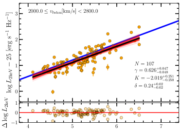
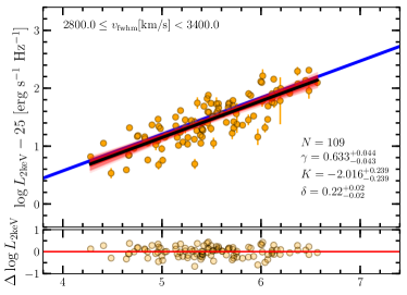
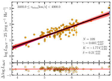
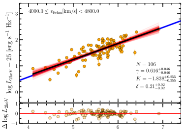
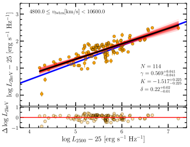
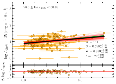
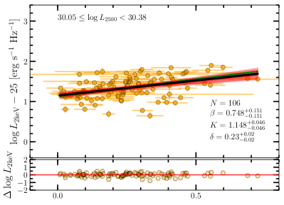
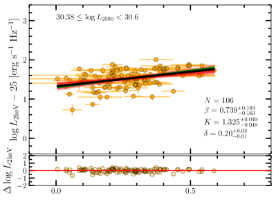
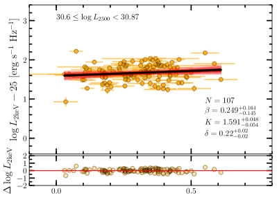
Figure 7 shows the $L_{\rm X}-L_{\rm UV}$ relationship in five intervals of $\upsilon_{\rm fwhm}$ in order to have approximately the same number of sources in each bin. The slope of the relation is statistically consistent within the uncertainties in all bins with the one of the clean sample as a whole (plotted with the blue solid line for reference). In Figure 8 we present five cuts of the $L_{\rm X}-\upsilon_{\rm fwhm}$ relation as a function of $L_{\rm UV}$. Overall, the estimates of the slope in each bin present large uncertainties, which are mainly driven by the fact that the $\upsilon_{\rm fwhm}$ measurements also display large error bars, thus part of the significance estimated on the observed correlations discussed in Section 3 may be affected. As a result, we can confirm the correlation between $L_{\rm X}$ and $\upsilon_{\rm fwhm}$ at the $3-5\sigma$ significance level only in the first three bins, while it is less than $2\sigma$ in the last two intervals. However, our employed fitting techniques perform better than other estimators in cases of large uncertainties (we refer to Kelly 2007 for a more detailed discussion).

A possible explanation for the tilted residuals in Figure 2 is likely due to the combination of high uncertainties on $\upsilon_{\rm fwhm}$ and the narrower range covered by $\upsilon_{\rm fwhm}$ with respect to both $L_{\rm X}$ and $L_{\rm UV}$. In fact, while $L_{\rm X}$ and $L_{\rm UV}$ cover roughly three orders of magnitude, the majority ($83\%$) of the selected quasars have $\upsilon_{\rm fwhm}$ values between 2000 and 5000 km/s in a relatively narrow range of $L_{\rm UV}$ and $L_{\rm X}$. This effect is clear in Figure 9 where we show $L_{\rm X}$ and $L_{\rm UV}$ as a function of $\upsilon_{\rm fwhm}$ for the selected quasar sample. The Pearson’s coefficient for the $L_{\rm X}-\upsilon_{\rm fwhm}$ and $L_{\rm UV}-\upsilon_{\rm fwhm}$ relations is 0.31 ($t-$value of $\sim 7\sigma$ on the slope) and 0.16 ($t-$value of $\sim 4\sigma$), respectively. We also point out that the estimated slope of the observed $L_{\rm X}-\upsilon_{\rm fwhm}$ relation is linked to $\hat{\gamma}$ and $\hat{\beta}$ as follows: $\beta=\hat{\gamma}\beta^{\ast}+\hat{\beta}$, where $\beta^{\ast}$ is the slope of the $L_{\rm UV}-\upsilon_{\rm fwhm}$ correlation.

The median signal-to-noise per resolution element of the optical spectra in the SDSS–DR7 quasar catalogue within the clean sample is in the range 7–13. High signal-to-noise spectra for a larger sample of quasars are required to not only accurately fit the shape of the line, thus improving $\upsilon_{\rm fwhm}$ measurements, but also to provide a better leverage at low/high luminosities.

(a)

(b)

(c)

(d)

(e)

Figure 8: Rest-frame monochromatic luminosities $\log L_{\rm X}$ against $\upsilon_{\rm fwhm}$ in bins (having roughly the same number of objects) of $L_{\rm UV}$. Keys as in Fig. 3. The best-fit regression line output of LINMIX_ERR is plotted with the green dashed line for reference.

Figure 9: Rest frame 2 keV and 2500Å monochromatic luminosities as a function of $\upsilon_{\rm fwhm}$. Keys as in Fig. 3. The best-fit regression line output of LINMIX_ERR is plotted with the green dashed line for reference. The Student’s t-test for the slope of the $L_{\rm UV}-\upsilon_{\rm fwhm}$ and $L_{\rm X}-\upsilon_{\rm fwhm}$ relations yields a significance that the slope is different from zero at approximately $4$ and $7\sigma$, respectively.