Simulation study of energy resolution, position resolution and $\pi^{0}$-$\gamma$ separation of a sampling electromagnetic calorimeter at high energies

Abstract

A simulation study of energy resolution, position resolution, and $\pi^{0}$-$\gamma$ separation using multivariate methods of a sampling calorimeter is presented. As a realistic example, the geometry of the calorimeter is taken from the design geometry of the Shashlik calorimeter which was considered as a candidate for CMS endcap for the phase II of LHC running. The methods proposed in this paper can be easily adapted to various geometrical layouts of a sampling calorimeter. Energy resolution is studied for different layouts and different absorber-scintillator combinations of the Shashlik detector. It is shown that a boosted decision tree using fine grained information of the calorimeter can perform three times better than a cut-based method for separation of $\pi^{0}$ from $\gamma$ over a large energy range of 20 GeV-200 GeV.

1 Introduction

Sampling calorimeters serve as a cost effective, yet highly performing, energy measurement device in many major high energy experiments and have been studied in the recent past for calorimetry in the future experiments. One such example is the CMS [1] experiment where the Shashlik detector was considered as a replacement of the existing PbWO₄ crystal calorimeter. In this study we use the material and geometry used in the CMS prototype for endcap calorimetry [2]. In this design LYSO is used as the sensitive detector. LYSO (cerium doped lutetium yttrium silicate) is a radiation hard, high light yield (about 4 times of BGO), high stopping power ($\rho$ = 7.4 g/cm³ , X₀ = 1.14 cm and R_Moliere = 2.07 cm) and fast response ($\tau$ =   40 ns) inorganic scintillator [3, 4].

For absorber, lead and tungsten are the two possible choices. For this study, the baseline option uses 4 mm thick lead layers interleaved with 2 mm thick LYSO. The alternative scenario considered uses 2.5 mm thick tungsten with 1.5 mm thick LYSO [5]. The scintillation light is read out using four wavelength shifting fibers going all the way through a Shashlik tower.

The following properties of the Shashlik calorimeter are studied:

1. the sampling resolution as a function of number of absorber/scintillator layers as well as total energy resolution;

2. position resolution of the impact point of photons on the calorimeter;

3. $\pi^{0}$/$\gamma$ separation using the information from the four fibers.

These are discussed in Sections 3, 4 and 5 respectively.

2 Simulation

A stand-alone detector setup consisting of alternative layers of absorbers (either 4 mm thick lead or 2.5 mm thick tungsten) and scintillators (2.0 mm or 1.5 mm thick LYSO) is defined in the framework of Geant4 [6]. Geant4 version 9.6.p02 is used with the physics list QGSP_FTFP_BERT. Light saturation effect is introduced through the use of Birk’s law  [7]:

$$w = \frac{k_{0}}{\left(1+k_{1}\cdot\left(\frac{dE}{dX}\right)+k_{2}\cdot\left(\frac{dE}{dX}\right)^{-1}\right)}$$

with $k_{0}$ = $0.883$, $k_{1}$ = $6.50\times 10^{-3}$ MeV${}^{-1}\cdot$g$\cdot$cm^-2 and $k_{2}$ = $-0.241$ MeV$\cdot$g${}^{-1}\cdot$cm² as measured in [8]. The weight factor $w$ is restricted in the range 0.1:1.0.

For studies of energy resolution, a single Shashlik tower, with no lateral segmentation and with each layer of transverse size $100\times 100$ cm² is used. The gun particle is directed along the central axis of the tower. The transverse size of the tower is sufficient to avoid any lateral leakage of the shower. Monochromatic electrons of energy 50, 150 and 200 GeV and monochromatic photons of energy 50, 100, 150, 200, 300, 400 and 500 GeV are produced for sampling resolution study as a function of number of layers. To study total energy resolution, electrons of energies 10, 20, 30, 50, 70, 100, 150, 200, 250, 300, 500, 700 and 1000 GeV are generated with 28 layers of absorber and 29 layers of scintillators. Ten thousand events are generated for each sample. Also, LYSO is considered to be undamaged by radiation (i.e. its attenuation length is taken to be 100 cm in this scenario).

For $\pi^{0}$-$\gamma$ separation studies, a detector setup with 28 layers of absorber and 29 layers of scintillators in a 11$\times$11 matrix is defined. Transverse size of each tower in each layer is chosen to be $14\times 14$ mm². Five fiber paths are defined of which the central fiber is for calibration and the other four fibers are at positions ($\pm$3.5 mm, $\pm$3.5 mm) with respect to the central axis. They are read out individually or to a combined output. The fibers are of diameter 1.6 mm and are inserted in holes of diameter 1.6 mm. The hit position is uniformly distributed in X and Y directions between $-$7 mm and $+$7 mm with respect to the centre of the central Shashlik tower. All the samples are generated using single particle gun with momentum along the Z direction. The gun is placed at a distance of 3.2 m from the calorimeter. For this study, photons and $\pi^{0}$’s of energy 10, 20, 30, 50, 70, 100, 150 and 300 GeV are shot at the calorimeter.

Energy deposited at a given point in the scintillator plate is shared unequally by the four fibers. The closer a fiber is to the point of impact of the photon, the higher its probability of collecting light is. Also the probability distribution of scintillator light among the fibers depends on the transmission coefficient of the scintillator and hence on integrated luminosity. This is estimated in a separate study [9] using SLitrani [10].

To validate the geometry, total energy deposit in the scintillator of the 11 $\times$ 11 matrix is looked at. As shown in Figure 1, the total energy deposit in the scintillator for $\pi^{0}$ and for $\gamma$ are very similar as expected.

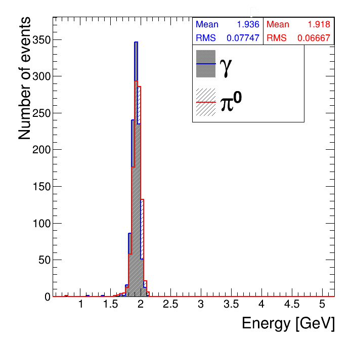
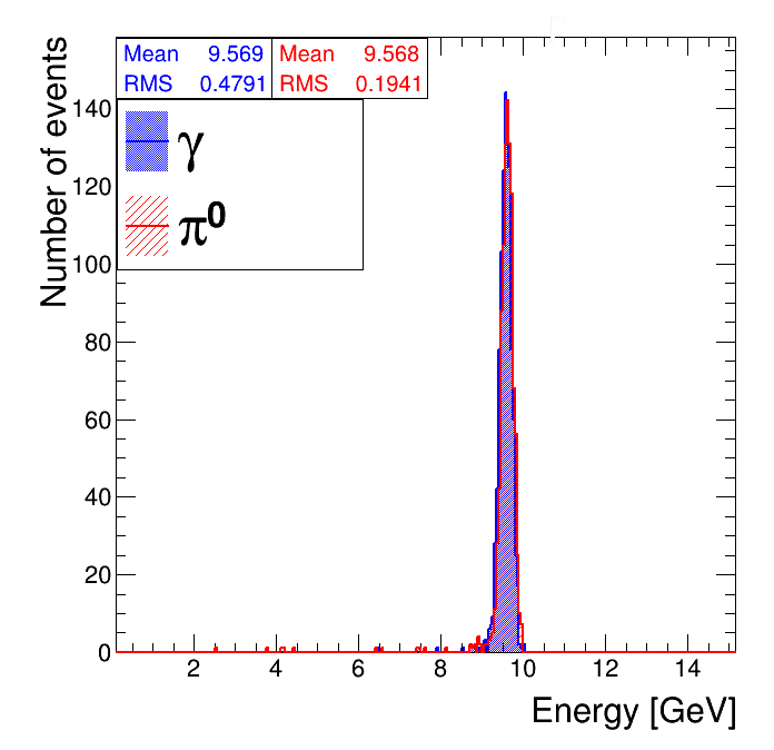
Figure 1: Total energy deposit in the scintillator of the 11 $\times$ 11 matrix for 10 GeV photons and $\pi^{0}$’s on the left and 50 GeV photons and $\pi^{0}$’s on the right. Blue shaded histogram is for photons and red hatched histogram is for $\pi^{0}$’s.

3 Energy resolution

The energy resolution in the Shashlik detector depends on the following factors:

1. energy leakage;

2. sampling fluctuation;

3. photo statistics;

4. electronic noise;

5. other sources which include contributions from pile-up and inter-calibration.

The second term is specific for a sampling calorimeter while the other terms contribute also to any homogenous calorimeter like the one used in the CMS experiment. Sampling resolution depends on the number of layers and the relative thickness between absorber and scintillator. A study is performed to obtain the optimum number of layers to achieve good sampling resolution.

3.1 Sampling resolution

For a given thickness of the absorber and sensitive layer and a given energy of electron/photon gun the sampling fraction is defined as

$$F_{s}=\frac{E_{S}}{E_{S}+E_{A}}$$ (3.1)

where E_S and E_A are the energies deposited in the scintillator layer and the absorber layer. The deposited energies in the scintillator as well as in the absorber layers follow Gaussian distribution. Figure 2 shows distributions of sampling fractions for 50 GeV and 100 GeV electrons in a configuration with 18 and 30 layers. The absorber in both the configurations is lead. Figure 3 shows similar distributions for 50 GeV and 100 GeV photons in a detector configuration with 18 and 30 layers. This configuration is with tungsten as absorber. Gaussian function provides good description of these distributions and the fits are used to estimate the sampling resolutions. One advantage of estimating the sampling resolution from $F_{S}$ and not estimating from the distribution of E_S is that E_S contains also the contribution to resolution due to leakage. In case of sampling fraction, the term due to leakage appears in the numerator and the denominator and gets canceled.

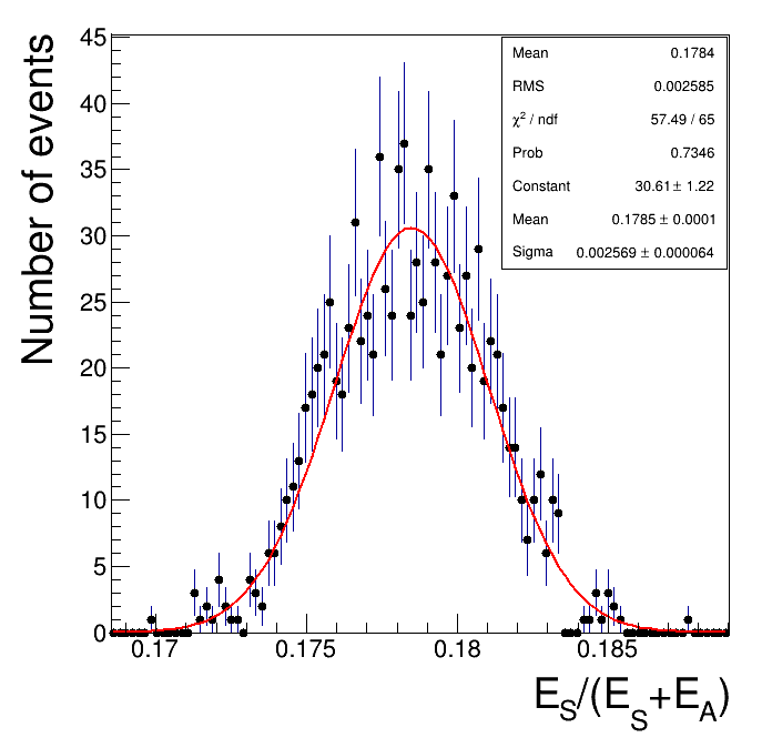
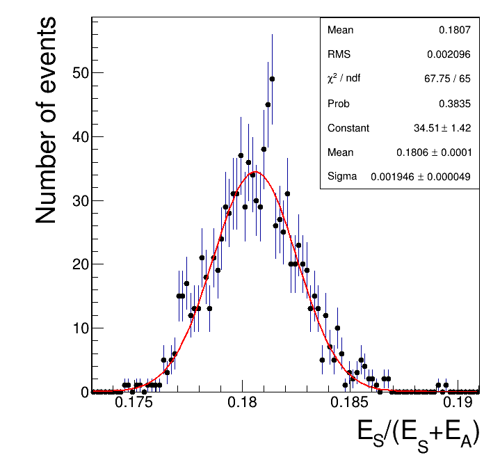
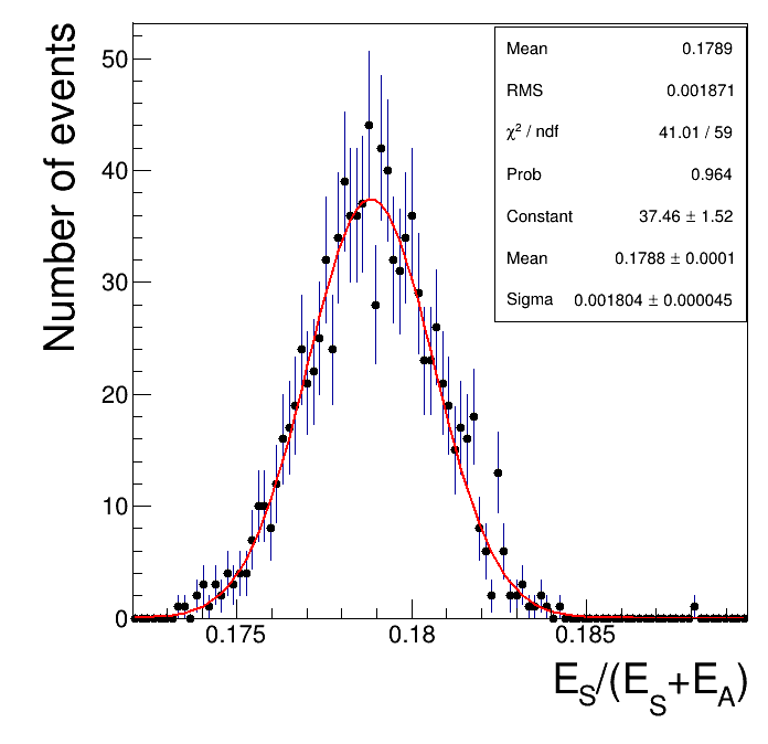
Figure 2: The top-left and bottom-left plots show the distributions of sampling fraction (F_S) for 18 layers and the top-right and bottom-right plots are for 30 layers. Top plots are for 50 GeV electrons and bottom plots are for 100 GeV electrons. These distributions are fitted to Gaussian distribution functions.

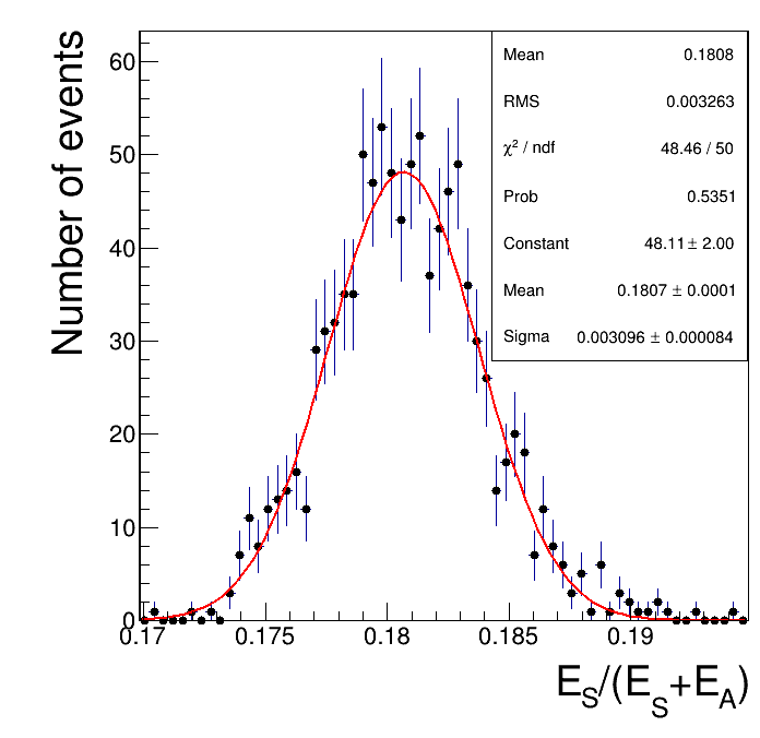
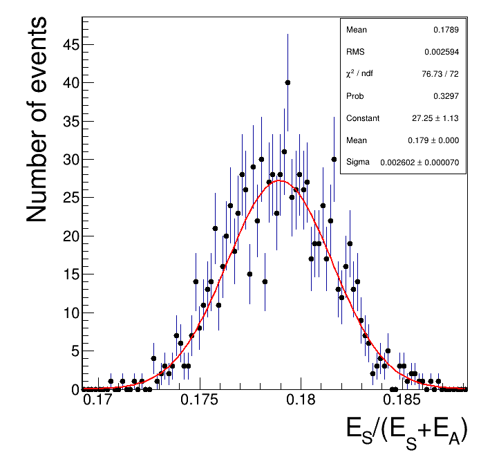
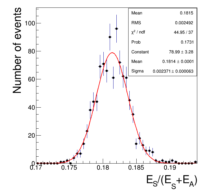
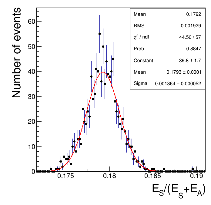
Figure 3: The top-left and bottom-left plots show the distributions of sampling fraction (F_S) for 18 layers and the top-right and bottom-right plots are for 30 layers. Top plots are for 50 GeV photons and bottom plots are for 100 GeV photons. These distributions are fitted to Gaussian distribution functions.

Fits are performed for each energy point and for each configuration. The fitted mean ($\bar{E}$) and the fitted width (${\sigma}$) of the Gaussian are used to estimate the energy resolution:

$$\textit{sampling-resolution}={\sigma}/\bar{E},$$ (3.2)

Figure 4 shows the sampling resolution for electrons and photons as a function of number of layers of absorber and scintillator. The following points are to be noted:

1. For same number of layers, sampling resolution becomes better as the energy increases.

2. As the number of layers increases, sampling resolution becomes better.

3. For number of layers larger than 28, the resolution becomes nearly flat. This corresponds to around 25 radiation lengths (X₀) in both the configurations (Pb-LYSO and W-LYSO), when longitudinal shower leakage is very small. Both configurations seem to give similar results within the statistics.

4. 25X₀ corresponds to $\sim$16.8 cm for Pb-LYSO and 11.8 cm in case of W-LYSO. If detector length is not an issue, then one can go with the less expensive configuration.

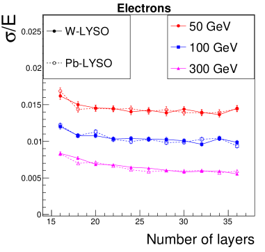
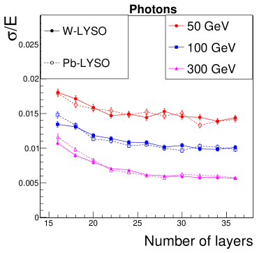
Figure 4: Plot on the left shows the sampling resolution of electrons of various energies for different number of layers of Pb-LYSO (dashed line with hollow triangle) and W-LYSO (solid line with solid circle). The plot on the right shows the same for photons.

3.2 Total energy resolution

Following are the terms contributing to the total energy resolution of the Shashlik detector:

Energy leakage:

To estimate this term, distributions of E_A+E_S are plotted in Figure 5 for different electron beam energies. The $\sigma/\bar{E}$ of this distribution gives the energy resolution due to leakage, where $\sigma$ is the measure of spread of the shower distribution and $\bar{E}$ is the mean of the shower distribution. It has low energy tail due to energy leakage because of limited length of the detector. Since the transverse size is 100 cm which is much larger than the Moliere radius ( 2.07 cm ) of the LYSO, transverse energy leakage is negligible. The distributions of E_A+E_S are fitted with the Crystal Ball (CB) function (as given in equation 3.3) because of the presence of low energy tail arising from shower leakage.

$$f(x;\alpha,n,\bar{E},\sigma) = N\times exp\left(\frac{-(x-\bar{E})^{2}}{2\sigma^{2}}\right),~{}for~{}\frac{x-\bar{E}}{\sigma}>-\alpha$$ (3.3)

$$= N\times A\times\left(B-\frac{x-\bar{E}}{\sigma}\right)^{-n},~{}for~{}\frac{x-\bar{E}}{\sigma}<-\alpha$$

where $N$ is the normalization factor and $\alpha$, $n$, $\bar{E}$, $\sigma$ are parameters of the fit. $A$ is given as:

$$A=\left(\frac{n}{|\alpha|}\right)^{n}\times exp\left(-\frac{|\alpha|^{2}}{2}\right)$$ (3.4)

and $B$ is given as:

$$B=\frac{n}{|\alpha|}-|\alpha|$$ (3.5)

Figure 5 shows the CB fit to the distribution of E_A+E_S. The CB parametrization fits the distribution well. The fitted mean of the CB function is taken as $\bar{E}$. To estimate the $\sigma_{68}$, 68$\%$ interval around $\bar{E}$, is constructed using the parameters of the CB fit. The interval is formed in such a way that for each side of the mean, the area covered is 68$\%$ of the area of that side. $\sigma_{68}$ is the half width of the interval as obtained by the above construction. Table 1 shows the values of $\sigma_{68}$ and $\bar{E}$ for different energies.

Energy	$\sigma_{68}$	$\bar{E}$
(GeV)	(GeV)	(GeV)
10	$0.23\pm 0.03$	$9.52\pm 0.01$
20	$0.29\pm 0.05$	$19.28\pm 0.01$
30	$0.29\pm 0.02$	$29.14\pm 0.02$
50	$0.35\pm 0.02$	$48.81\pm 0.03$
70	$0.40\pm 0.03$	$68.47\pm 0.03$
100	$0.49\pm 0.03$	$98.04\pm 0.04$
200	$0.66\pm 0.06$	$196.22\pm 0.05$
300	$1.00\pm 0.09$	$294.44\pm 0.10$
500	$2.17\pm 0.32$	$490.95\pm 0.12$
1000	$5.53\pm 0.81$	$980.97\pm 0.32$

Table 1: The values of $\sigma_{68}$ and $\bar{E}$ of the distribution of E_A+E_S for electrons with different energies.

The values of $\sigma_{68}/\bar{E}$ are then plotted as a function of energy. Fluctuations due to energy leakage are parametrized using Grindhammer-Peter’s parametrization [12]:

$$\sigma_{leakage}(\ln(E/E_{c}))=(s1+s2\times\ln(E/E_{c}))^{-1},$$ (3.6)

where $E_{c}$ is the critical energy and is dependent on the material of the detector. The above equation is expanded up to the third power in $\ln(E/E_{c})$ and the resolution due to leakage is fitted with a function of type $p_{0}+p_{1}\times\ln E+p_{2}\times(\ln E)^{2}+p_{3}\times(\ln E)^{3}$. Fitted values of $p_{0}$, $p_{1}$, $p_{2}$ and $p_{3}$ are shown in Table 2.

parameter	Fitted value
$p_{0}$	$0.118\pm 0.010$
$p_{1}$	$-0.058\pm 0.007$
$p_{2}$	$(9.8\pm 1.6)\times 10^{-3}$
$p_{3}$	$(-5.3\pm 1.2)\times 10^{-4}$

Table 2: Fitted values of the parameters when $\sigma_{68}/\bar{E}$ due to leakage is fitted with function $p_{0}+p_{1}\times\ln E+p_{2}\times(\ln E)^{2}+p_{3}\times(\ln E)^{3}$.

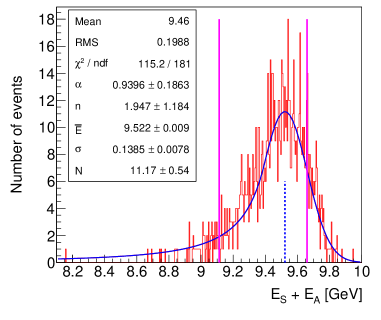
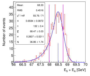
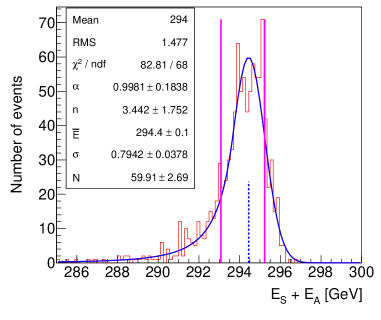
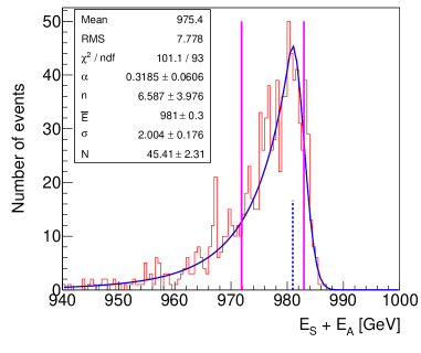
Figure 5: The distribution of E_S+E_A for 10 GeV electrons on the top-left; 70 GeV electrons on top-right; 300 GeV electrons on bottom-left and 1000 GeV electrons on bottom-right. The blue curves show the Crystal Ball fit to the distributions. The pink lines show the $\sigma_{68}$ which is the 68$\%$ interval constructed as discussed in the text and the blue dotted lines show the fitted Crystal Ball mean.

Sampling fluctuation:

It is estimated for each energy point exactly the same way as described in the previous sub-section. This is done for a 28 layer configuration. The distribution of $\sigma/\bar{E}$ is plotted as a function of energy and fitted with a function of type $p_{0}/\sqrt{E}$. Fitted value of $p_{0}$ comes out to be 0.104 $\pm$ 0.001 .

Photo-statistics:

To estimate the contribution due to photo-statistics, the energy collected in all the scintillator layers is converted to the number of photo-electrons (p.e.) in the photo-detector. The total number of p.e. from the scintillator is

$$N_{pe}=\Sigma E_{i}~{}\times~{}LE~{}\times~{}LY$$ (3.7)

where $E_{i}$ is the energy deposit in i’th layer, $LE$ is the light collection efficiency and $LY$ is the light yield. The light yield is different for different materials [13]. The photo-statistics contribution can vary depending on the light yield of the material. Average light collection efficiency (LE) is taken to be 0.5% [14] for each layer. (Only a small fraction of scintillation photons is collected by the fibers which go through the holes of each layer and thus leads to such a low efficiency). The distribution of p.e. follows Poisson distribution and hence the fluctuation has a $\sqrt{LY}$ dependence. The distributions of $\sigma/\bar{E}$ in Figure 7 are fitted with a function of type $p_{0}/\sqrt{LY}$. The fit yields $p_{0}$ to be 0.1068 $\pm$ 0.0001 for 100 GeV electron beam energy. Figure 7 shows the distribution of $\sigma/\bar{E}$ as a function of incident energy for different values of $LY$. Fits of these distributions to functions of the the type $p_{0}/\sqrt{E}$ yield $p_{0}$ to be 0.0171 $\pm$ 0.0001 for light yield value of 4000 p.e./MeV.

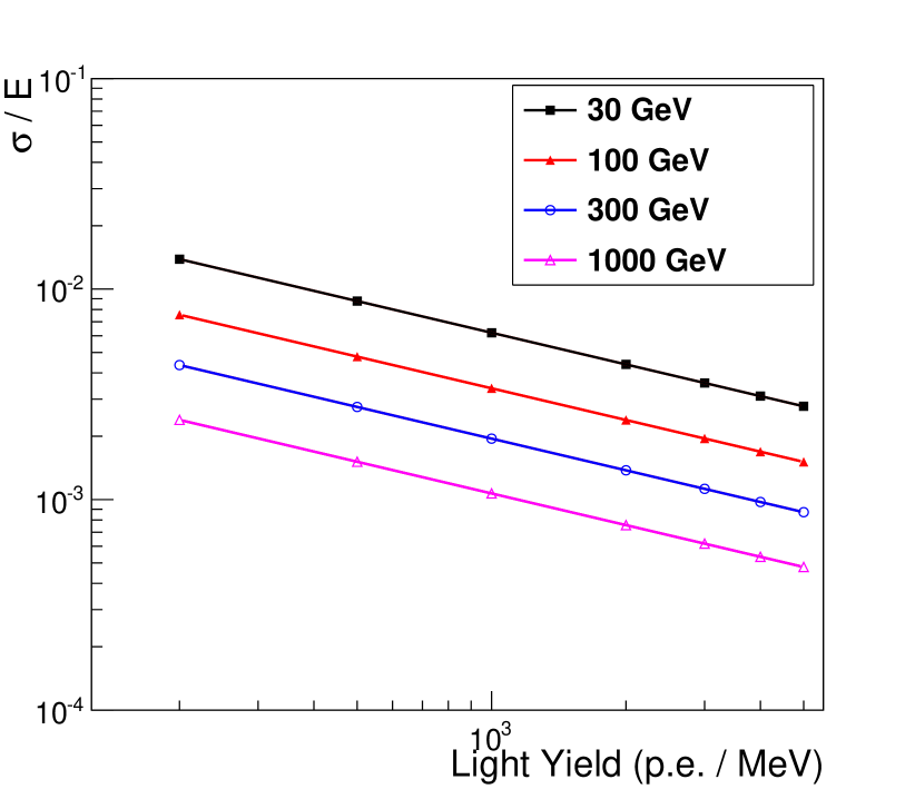
Figure 6: Photo-statistics contribution as a function of light yield (LY) for different beam energies

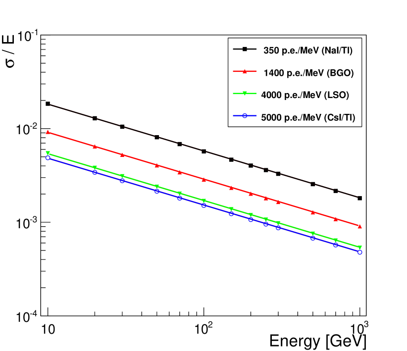
Figure 7: Photo-statistics contribution as a function of energy for different light yields.

Electronic noise:

Contribution of electronic noise in the photo-detectors to the energy resolution depends on the fluctuation in the number of photo electrons contributing to the noise. It varies depending on the read-out scheme. Figure 9 shows the noise distribution as a function of mean number of p.e. corresponding to electronic noise for different beam energies. Fits to the energy resolution $\sigma/\bar{E}$ to a function of the type $p_{0}\times p.e.$ yield a value of $p_{0}$ to be $(2.8\pm 0.1)\times 10^{-6}$ for 100 GeV electron beam energy.

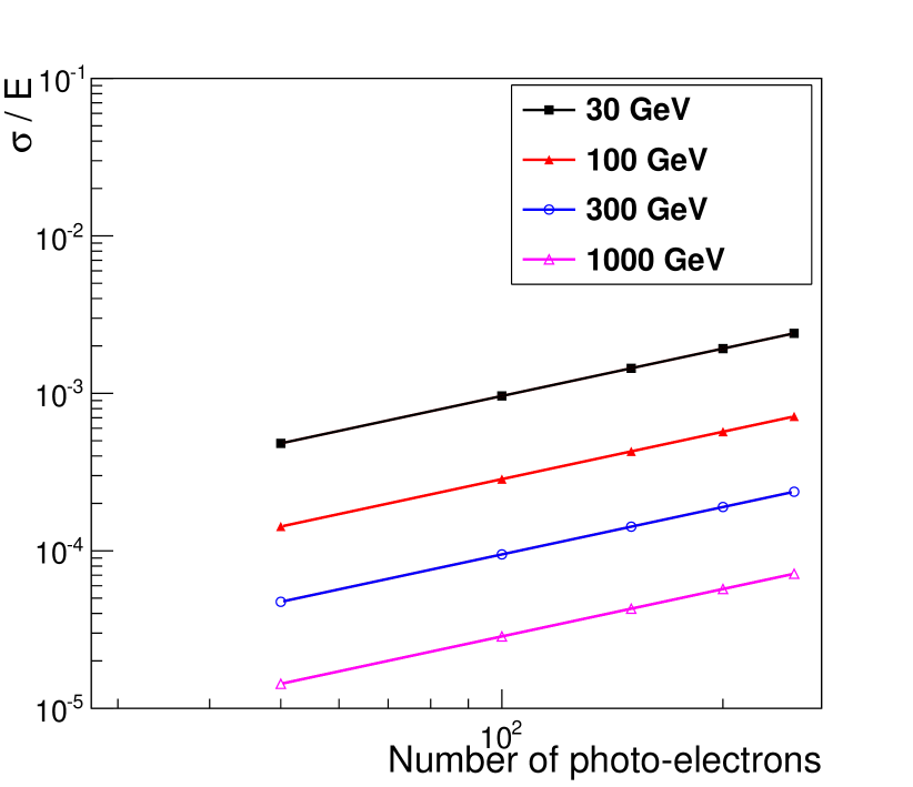
Figure 8: Noise contribution as a function of photo-electrons for different beam energies.

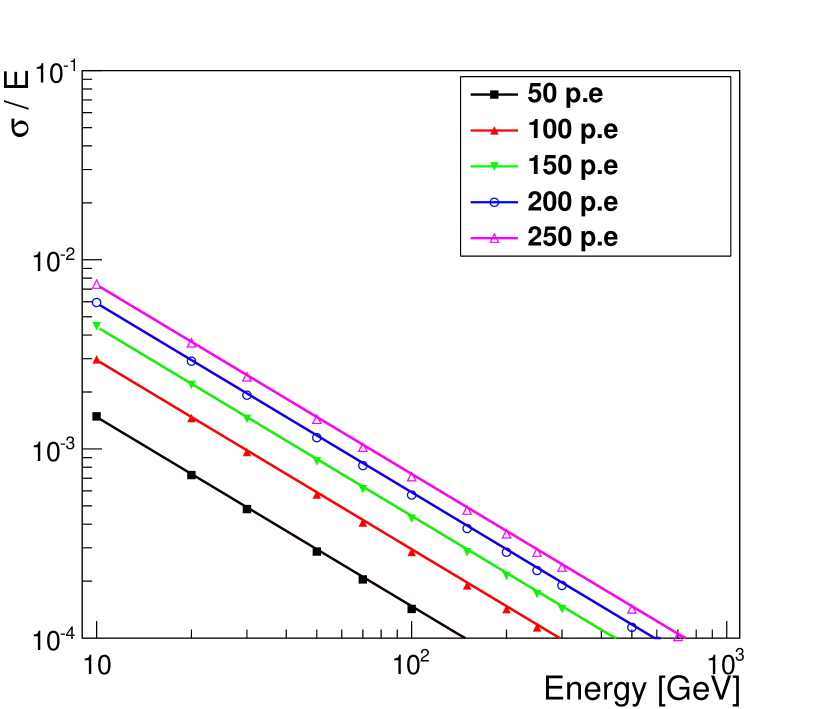
Figure 9: Noise contribution as a function of energy for different number of photo-electrons.

Figure 9 shows the distributions of $\sigma/\bar{E}$ as a function of energy and are fitted with functions of the type $p_{0}/E$ for for different numbers of mean photo-electrons. Fitted value of $p_{0}$ comes out to be 0.0442 $\pm$ 0.0002 for 150 as mean number of photo-electrons.

Total energy resolution:

Total energy resolution is the sum (in quadrature) of the above four terms. The distribution of $\sigma/\bar{E}$ is plotted as a function of beam energy in Figure 10 for light yield value of 4000 p.e./MeV and mean noise of 150 p.e. The energy resolution is fitted with a function of the type

$\sqrt{\left(p_{0}/\sqrt{E}\right)^{2}+\left(p_{1}/E\right)^{2}+\left(p_{2}+p_{3}\times\ln E+p_{4}\times(\ln E)^{2}+p_{5}\times(\ln E)^{3}\right)^{2}}$.

and the fitted parameters are shown in Table 3. Figure 10 also shows contributions of each of the term as given above. It can be seen that the parameters of the total fit are in agreement with the individual parameters obtained by fitting all the terms (i.e. leakage, sampling, statistics and noise) of the resolution individually. The parameter, $p_{0}$ has contribution from both the terms, sampling and statistics. But the major contribution comes from sampling and hence the fitted parameter $p_{0}$ is closer to the fitted value of the sampling term.

parameter	Fitted value
$p_{0}$	0.103 $\pm$ 0.006
$p_{1}$	0.087 $\pm$ 0.056
$p_{2}$	0.118 $\pm$ 0.002
$p_{3}$	-0.058 $\pm$ 0.001
$p_{4}$	$(9.8\pm 0.1)~{}\times 10^{-3}$
$p_{5}$	$(-5.3\pm 0.1)~{}\times 10^{-4}$

Table 3: Table showing fitted values of the parameters when $\sigma/\bar{E}$ of total energy resolution is is fitted with function $\sqrt{\left(p_{0}/\sqrt{E}\right)^{2}+\left(p_{1}/E\right)^{2}+\left(p_{2}+p_{3}\times\ln E+p_{4}\times(\ln E)^{2}+p_{5}\times(\ln E)^{3}\right)^{2}}$.

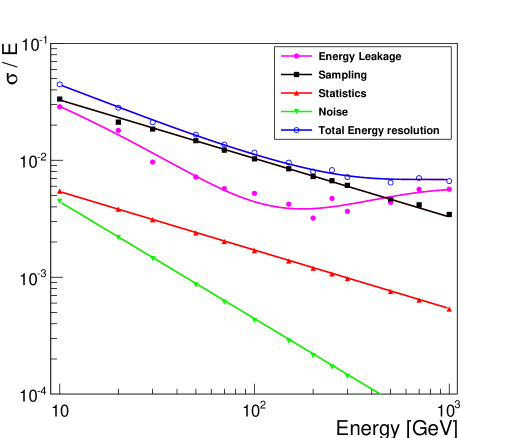
Figure 10: Contributions of each term to the total resolution. Points are the actual points as a function of energy and lines are the fitted functions.

Finally, to check the effect of this detector resolution on the mass resolution of the Higgs boson, 10000 events are generated where the Higgs boson is produced via gluon gluon fusion, and decays to a photon pair. Higgs mass is taken to be 125 GeV. In order to mimic the effect of the Shashlik detector, energy of each photon was smeared with the parameters as given in Table 3 in the following way:

1. a resolution term, $\sigma/$E is calculated for each of the photons using the parameters of Table 3 and the expression given in there;

2. a Gaussian random number is generated with mean 1 and $\sigma_{gaus}=\sigma/$E;

3. energy and momentum of each photon is multiplied with the above random number;

4. the diphoton mass is fitted with a Gaussian function. The $\sigma$ from the fit is taken as the estimate of resolution of Higgs mass.

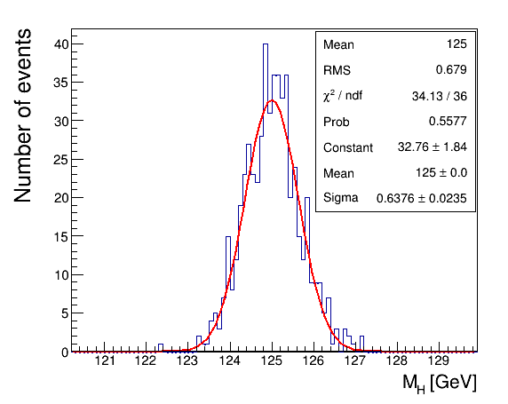
Figure 11: Resolution on Higgs mass with a Shashlik ECAL and with both the photons in the endcap electromagnetic calorimeter.

Figure 11 shows the Gaussian fit to Higgs mass, when both the photons are in the endcap electromagnetic calorimeter, obtained using the above procedure. The fitted $\sigma$ is estimated to be $0.64\pm 0.02$.

4 Position resolution

When a particle hits the electromagnetic calorimeter, its deposited energy gets distributed in the hit tower as well as the towers around it. The hit position can be estimated from the weighted mean of the position of the towers in which energy has been deposited, where the weights are proportional to the energy deposited in the towers (so that higher the energy, more is the weight and hence more likely that the particle has hit that tower). This method of estimating the position is called the center of gravity (COG) method. The equations used to estimated coordinates in this way are given in Equation 4.1.

$$x_{meas} = \Sigma x_{i}\times E_{i}/\Sigma E_{i}$$

$$y_{meas} = \Sigma y_{i}\times E_{i}/\Sigma E_{i}$$ (4.1)

Here, the sum is over the 3 $\times$ 3 array of towers, if a combined signal from the four fibers are read out for each tower, or it is over 3 $\times$ 3 $\times$ 4 array of fibers, if individual fiber information is used. Figures 12 and 13 show the true impact point $x_{true}$ and $y_{true}$ as a function of the measured coordinates $x_{meas}$ or $y_{meas}$ for 50 GeV and 150 GeV photons. The resulting distributions show deviations from linearity and roughly follows an S-shape. This feature is observed for combined as well as individual fiber readouts.

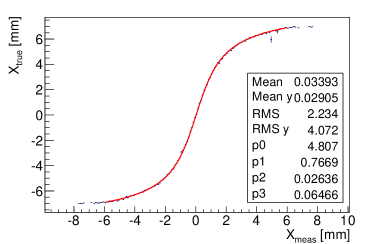
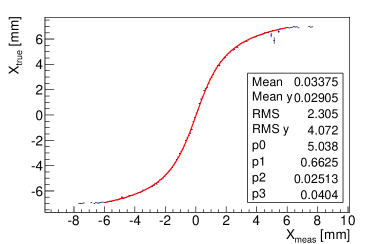
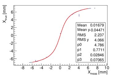
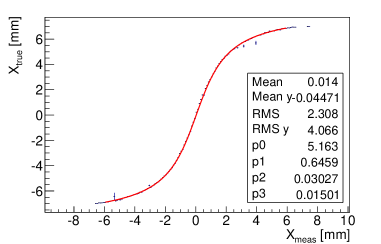
Figure 12: 2-D distribution of x_true versus x_meas for photons of energy 50 GeV (top plots) and 150 GeV (bottom plots) when linear weights are used to estimate the COG. The relation between x_meas and x_true is fitted with a S-shaped curve as parametrized in the Equation 4.3 and shown by the red curve in the figure. The left (right) figures refer to cases when combined (individual) fiber information is used.

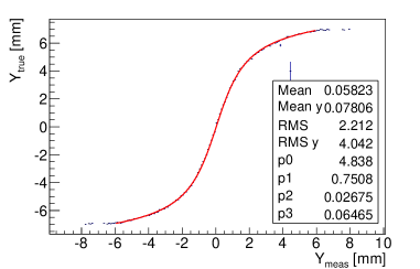
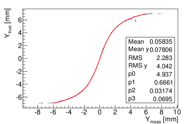
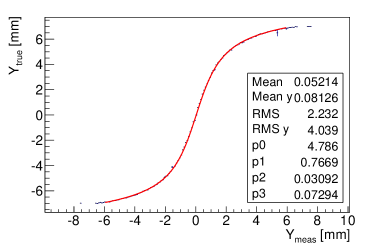
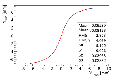
Figure 13: 2-D distribution of y_true versus y_meas for photons of energy 50 GeV (top plots) and 150 GeV (bottom plots) when linear weights are used to estimate the COG. The relation between y_meas and y_true is fitted with a S-shaped curve as parametrized in the Equation 4.3 and shown by the red curve in the figure. The left (right) figures refer to cases when combined (individual) fiber information is used.

Some features of the S-shape curve are summarized below:

1. At the center, x_true (y_true) = x_meas (y_meas). This is because the deposited energy is mostly contained in the central tower.

2. On moving away from the center in either direction, x_true (y_true) $>$ x_meas (y_meas). There is an exponential fall in the spread of the energy for other towers. So linear weights E_i give more weight to the hit tower and hence the position is not correctly determined.

3. At the edge (in this case at $\pm$6 mm), the energy is distributed equally in the adjacent towers and roughly equal weight is given to them and hence x_true (y_true) again becomes x_meas (y_meas).

Above three points essentially summarize why the S-shape arises. Instead of linear weights, log weights of energy fraction are also tried. Since the energy falls off as an exponential, the log weights compensate the exponential decrease and hence the estimated position is closer to the true one. Equation 4.2 shows the relations used to estimate the coordinates of the hit point with log weights. This equation depends highly on the value of $w_{0}$. The optimum value of $w_{0}$ depends on whether individual or combined fiber information is used. Figures 14 and 15 show the 2-D distribution of $x_{true}$ ($y_{true}$) VS $x_{meas}$ ($y_{meas}$) for 50 GeV and 150 GeV photons when log weights are used for the two cases of using combined or individual fiber information.

$$x_{meas} = \Sigma x_{i}\times w_{i}/\Sigma w_{i}$$

$$y_{meas} = \Sigma y_{i}\times w_{i}/\Sigma w_{i}$$

$$w_{i} = Max(0,w0+\ln(E_{i}/E_{T}))$$ (4.2)

where $w_{0}$ $=$ 4.7 for combined fiber information and $w_{0}$ $=$ 6 for individual fiber information.

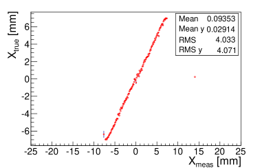
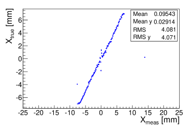
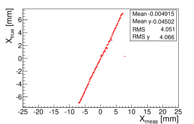
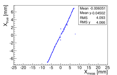
Figure 14: 2-D distribution of x_true versus x_meas for photons of energy 50 GeV and 150 GeV when log weights are used to estimate the COG as given in Equation 4.2. The left (right) figures refer to cases when combined (individual) fiber information is used.

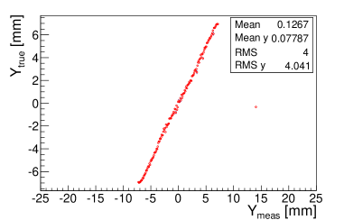
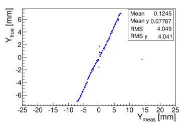
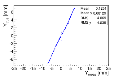
Figure 15: 2-D distribution of y_true versus y_meas for photons of energy 50 GeV and 150 GeV when log weights are used to estimate the COG as given in Equation 4.2. The left (right) figures refer to cases when combined (individual) fiber information is used.

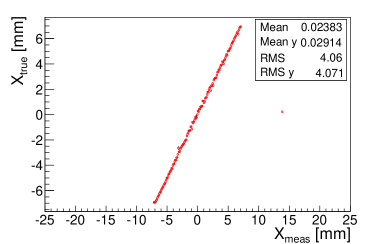
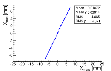
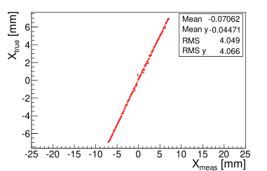
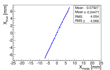
Figure 16: 2-D distributions of x_true versus S-shape corrected x_meas for photons of energy 50 GeV (top) and 150 GeV (bottom) when linear weights are used to estimate the COG as given in Equation 4.1. The left (right) figures refer to cases when combined (individual) fiber information is used.

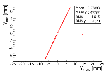
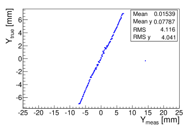
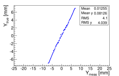
Figure 17: 2-D distributions of y_true versus S-shape corrected y_meas for photons of energy 50 GeV (top) and 150 GeV (bottom) when linear weights are used to estimate the COG as given in Equation 4.1. The left (right) figures refer to cases when combined (individual) fiber information is used.

For this analysis, linear weights are used to estimate the position of COG. These S-shape curves are then fitted with a function of the form

$$x_{true} = P_{0}\times\tan^{-1}{(P_{1}\times(x_{meas}-P_{2}))}+P_{3}\times{(x_{meas}-P_{2})}$$

$$y_{true} = P_{4}\times\tan^{-1}{(P_{5}\times(y_{meas}-P_{6}))}+P_{7}\times{(y_{meas}-P_{6})}$$ (4.3)

Figures 12 and 13 show how the fitted functions for X and Y look like for 50 GeV and 150 GeV photons. Using these fitted functions, the $x_{meas}$ ($y_{meas}$) are corrected so that the measured position coordinates are nearer to the true ones, i.e., $x_{true}$ ($y_{true}$). Fitted parameters differ slightly depending on the energy of the photon. For simplicity fitted parameters from 50 GeV photons are used to fit all energy particles and to obtain S-shape corrected $\overline{x}$ and $\overline{y}$. These S-shaped corrected positions are then used in Equation 5.2 as $\overline{x}$ and $\overline{y}$. Figure 16 shows the S-shape corrected X position of 50 GeV and 150 GeV photons for both the cases of combined and individual fiber information. Similarly, Figure 17 shows the S-shape corrected Y position of 50 GeV and 150 GeV photons.

Position resolution is studied from samples of photons produced with impact points randomly distributed on the front face of the module. The difference between the true and measured position along X and Y directions are plotted. These distributions follow roughly a Gaussian shape. The RMS of these distributions is used to estimate the position resolution of these photons. Figure 18 shows position resolution as a function of photon energy for three different scenario: (a) position with linear weighting in energy; (b) S-shape corrected position with linear weighting in energy; and (c) position with logarithmic weighting. Position resolution improves as a function of the photon energy in all three cases.

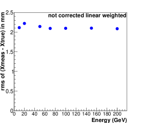
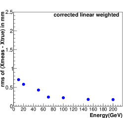
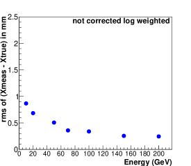
Figure 18: Position resolution for photons in a Shashlik detector as a function of photon energy with position reconstructed using linear weighting in energy (a); S-shape corrected position with linear weighting in energy (b); and position with logarithmic weighting (c).

Position resolution is quite large and is related to the lateral size of the tower if one simply uses linear weighting in energy in determining the impact point and without any further correction. With S-shape correction, the resolution improves significantly. The resolution is 0.70 mm for photons at 10 GeV and it improves with energy becoming 0.22 mm at 200 GeV. Logarithmic weighting takes care of the correction to some extent and even without any further correction the resolution is 0.87 mm at 10 GeV and 0.34 mm at 200 GeV. A precise measurement of the impact position is extremely useful for $\pi^{0}$/$\gamma$ separation.

5 $\pi^{0}$/$\gamma$ separation

An important measure of the performance of an electromagnetic calorimeter used in a high energy physics experiment is its ability to separate between photons and $\pi^{0}$s. In high energy collisions any final state with photons has a background contribution from jets which fake photons. This is because $\pi^{0}$’s in jets decay to 2$\gamma$’s almost 99.9% of the time. For decays of a high energy $\pi^{0}$, the angle between the two photons can become comparable with or smaller than the granularity of the calorimeter. It is very difficult to separate the photons from such a decay from photons which are coming either from the interaction vertex or from radiation off charged leptons.

In this study, the idea of exploiting the information from the four fibres for $\pi^{0}$/$\gamma$ separation has been investigated. The idea behind using information from all the four fibers individually is that a larger fraction of the deposited energy from a single photon will be collected by the fiber which is closest to the impact point, while $\pi^{0}$, decaying to a pair of photons will have two impact points on the Shashlik detector and the sharing of light among the fibers will significantly increase.

5.1 Shower shapes

In general, the lateral shower profile tends to be broader for photons coming from $\pi^{0}$ compared to that of prompt photons. This holds true for lower energy $\pi^{0}$’s (less than 100 GeV). Therefore shower shape variables are useful for discriminating between $\pi^{0}$’s and photons. For all shower shape variables, the tower with maximum energy deposit is first identified and then the shape parameters are formed around it. The following shape variables are considered:

$S1/S9$:

This ratio makes use of $S1$, the maximum energy deposited in a tower, and $S9$, the energy deposited in 3$\times$3 array around the maximum energy deposited tower. Figure 19 shows the array of 3$\times$3 towers formed around the maximum energy deposited tower and the distribution of $S1/S9$ for 50 GeV, 70 GeV and 150 GeV photons and $\pi^{0}$’s.

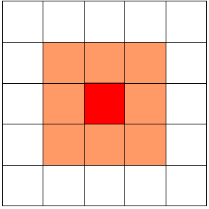
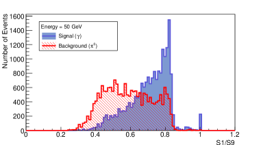
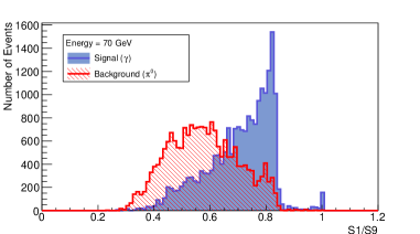
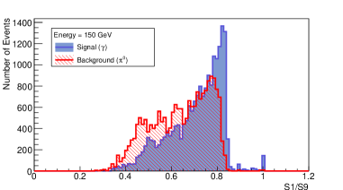
Figure 19: The top left diagram shows 3$\times$3 array of towers in light orange color and the maximum energy deposited tower in red color. The top-right figure shows the distribution of S1/S9 for 50 GeV photons and $\pi^{0}$’s. Similar distribution for 70 GeV photons and $\pi^{0}$’s is on the bottom left; and 150 GeV photons and $\pi^{0}$’s is on the bottom right. The blue hatched histogram is for photons and the red hatched histogram is for $\pi^{0}$’s [17].

$S1/S4$:

This ratio uses $S4$, the energy deposited in 2$\times$2 array including the maximum energy tower. Four possible 2$\times$2 arrays are possible which include the maximum energy tower. The combination which corresponds to the largest sum total energy is used in determining the ratio. Figure 20 shows the four possible combinations of 2$\times$2 array of towers and the distributions of $S1/S4$ for 50, 70 and 150 GeV photons and $\pi^{0}$’s.

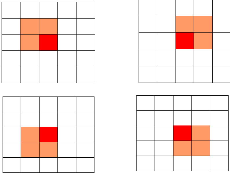
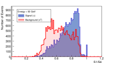
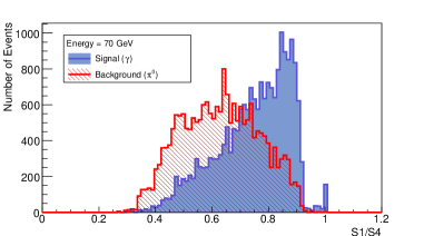
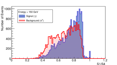
Figure 20: The top left diagram shows the four possible combinations of 2$\times$2 arrays which can be formed including the maximum energy tower. The top right figure shows the distribution of S1/S4 variable for 50 GeV photons and $\pi^{0}$’s. The bottom left and right plots correspond to 70 GeV and 150 GeV photons and $\pi^{0}$’s. The blue hatched histogram is for photons and the red hatched histogram is for $\pi^{0}$’s [17].

2-D distribution of $F_{16}$ vs $F_{9}$:

The variables, $F_{9}$ and $F_{16}$, are defined through equation 2-D distribution of $F_{16}$ vs $F_{9}$:.

$$F_{9} = \frac{S9-S1}{S9}$$

$$F_{16} = \frac{S16-S4}{S16}$$ (5.1)

where $S16$ is the energy deposited in the 4$\times$4 array of towers that is centered on the 2$\times$2 array of towers with the maximum energy, among the four possible combinations as explained above. Figure 21 shows the diagrammatic view of 4$\times$4 array of towers around the 2$\times$2 array of towers and the 2-D distribution of F₁₆ and F₉ for 50, 70 and 150 GeV photons and $\pi^{0}$’s.

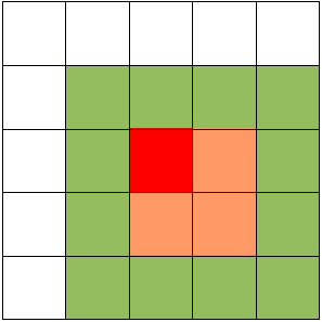
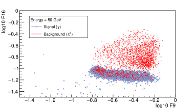
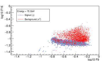
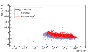
Figure 21: The top left diagram shows the 4$\times$4 arrays of towers formed around that array of 2$\times$2 towers which has maximum energy of the four possible combinations as explained in the text. The top-right plot shows the 2-D distribution of F₁₆ along the Y axis and F₉ along the X axis for 50 GeV photons and $\pi^{0}$’s. Similar plots at 70 GeV and 150 GeV are at the bottom left and at the bottom right respectively. The blue points are for photons and the red points are for $\pi^{0}$’s [17].

The performance of the variables $S1/S9$, $S1/S4$ and $F_{16}$ vs $F_{9}$ are summarized below:

• Shower shape variables $S1/S9$ and $S1/S4$ lose the sensitivity for $\gamma$/$\pi^{0}$ separation at energies above 70 GeV;

• The 2-D distribution of $F_{16}$ vs $F_{9}$ performs better for 70 GeV $\gamma$/$\pi^{0}$ discrimination compared to $S1/S9$ and $S1/S4$. But again it loses power for discrimination at energies above 70 GeV.

5.2 Moment analysis

This analysis is based on the consideration that when the $\pi^{0}$ decays to two $\gamma$’s, the shower tends to be elliptical, as shown in Figure 22, whereas for a prompt photon the spread in X and Y will tend to be similar, because the shower spreads uniformly in all the directions. The above holds true for photons not converted before they reach the front face of the tower and when there is no magnetic field. Early conversion and passage through magnetic field make the decay topology more complicated.

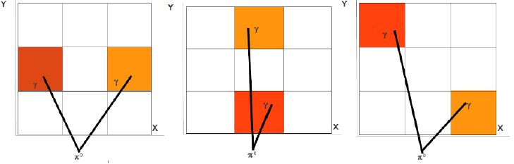
Figure 22: Diagram showing three different topologies of a $\pi^{0}$ decay.

The ratio of major axis of the ellipse to its minor axis or vice-versa is utilized to distinguish between photons and $\pi^{0}$’s. For $\pi^{0}$’s, the ratio between the two axes is expected to be away from 1, whereas, for photons, it is expected to be close to 1. To get the values of the length of both of the axis of the shower, a covariance matrix can be formed with the quantities as given in Equation 5.2. The eigenvalues of this matrix is related to the length of the shower axis. The spread is calculated from the point of impact of the photon or the $\pi^{0}$. The point of impact is estimated using the COG method and correcting for the S-shape as discussed in Section 4. The 2$\times$2 matrix is formed in each event as follows:

$$M = \left|\begin{array}[]{cc}\sigma^{2}_{x}&\sigma^{2}_{xy}\\ \sigma^{2}_{xy}&\sigma^{2}_{y}\\ \end{array}\right|$$

The definition of each of the terms of the above matrix is given below

$$\sigma^{2}_{x} = \Sigma(x_{i}-\overline{x})^{2}\times w_{i}/\Sigma w_{i}$$

$$\sigma^{2}_{y} = \Sigma(y_{i}-\overline{y})^{2}\times w_{i}/\Sigma w_{i}$$

$$\sigma^{2}_{xy} = \Sigma(x_{i}-\overline{x})\times(y_{i}-\overline{y})\times w_{i}/\Sigma w_{i},$$ (5.3)

where $\overline{x}$ and $\overline{y}$ are the S-shape corrected Center of Gravity (COG) positions of the shower in X and Y, and $w_{i}$ are the weights associated with each contribution. This matrix is then diagonalized to extract the eigenvalues, $\lambda_{+}$ and $\lambda_{-}$. The ratio of eigenvalues of this matrix, $\lambda_{-}$/$\lambda_{+}$ or $\lambda_{+}$/$\lambda_{-}$ measures the eccentricity of the energy distribution and is used to discriminate direct $\gamma$ from $\pi^{0}$.

There are two ways in which the weights, $w_{i}$ are formed:

Linear weights, $w_{i}$:

Here the weights, $w_{i}$ are given by Equation Linear weights, $w_{i}$::

$$x_{meas} = \Sigma x_{i}\times w_{i},$$

$$y_{meas} = \Sigma y_{i}\times w_{i},$$

$$w_{i} = E_{i}/\Sigma E_{i}.$$ (5.4)

Logarithmic weights, $w_{i}$:

In this case, the weights, $w_{i}$ are given by the Equation Logarithmic weights, $w_{i}$:

$$x_{meas} = \Sigma x_{i}\times w_{i}/\Sigma w_{i},$$

$$y_{meas} = \Sigma y_{i}\times w_{i}/\Sigma w_{i},$$

$$w_{i} = Max(0,w_{0}+\ln(E_{i}/E_{T})),$$ (5.5)

where $w_{0}$ is related to the threshold for the towers below which the towers are not included in the sum, and $E_{T}$ is the total energy deposited in the array.

There are two ways in which the covariance matrix can be constructed:

1. use combined information of all four fibers in a given tower [Coarse grain information];

2. use information from individual fiber in a given tower [Fine grain information].

5.2.1 Coarse grain Information

In this case, E_i refers to the total energy recorded by $i^{th}$ tower (i=1-9 for $3\times 3$ array) and $x_{i}$ and $y_{i}$ are the X and Y coordinates of the center of $i^{th}$ tower. E_i is obtained by summing the energy recorded from all four fibers of the $i^{th}$ tower. Both linear and log weights are used in the determination of the impact point. In case of log weights, $w_{0}$ is set to be 4.7. Figures 23, 24 and 25 show the ratio of $\lambda_{-}$/$\lambda_{+}$ for photons and $\pi^{0}$’s at 50 GeV, 70 GeV and 150 GeV. These plots clearly demonstrate that log weights improve the discriminating power between photons and $\pi^{0}$’s over linear weights.

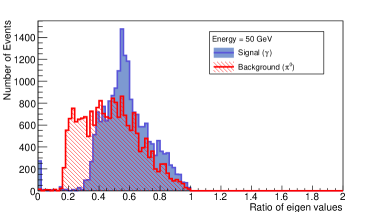
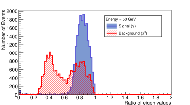
Figure 23: Distribution of $\lambda_{-}$/$\lambda_{+}$ for photons and $\pi^{0}$’s of 50 GeV for the case of coarse grain information (no information from individual fibers used). The plot on the left is done with linear weights for determining the impact point while the plot on the right is done with the log weights.

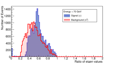
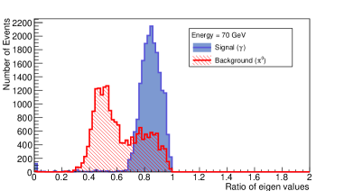
Figure 24: Distribution of $\lambda_{-}$/$\lambda_{+}$ for photons and $\pi^{0}$’s of 70 GeV for the case of coarse grain information (no information from individual fibers used). The plot on the left is done with linear weights for determining the impact point while the plot on the right utilizes log weights.

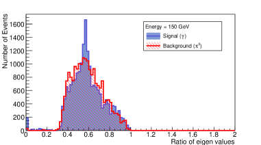
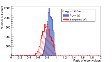
Figure 25: Distribution of $\lambda_{-}$/$\lambda_{+}$ for photons and $\pi^{0}$’s of 150 GeV for the case of coarse grain information (no information from individual fibers used). The plot on the left is done with linear weights for determining the impact point while the plot on the right utilizes log weights.

5.2.2 Fine grain information

For fine grain information E_i refers to the energy recorded by $i^{th}$ individual fiber (i=1-36 for $3\times 3$ array) and $x_{i}$ and $y_{i}$ are the X and Y coordinates of the $i^{th}$ fiber. The impact point is determined with both linear weights and log weights.

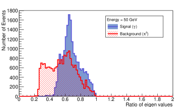
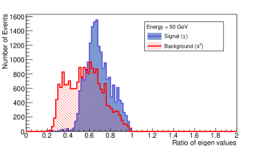
Figure 26: Distribution of $\lambda_{-}$/$\lambda_{+}$ for photons and $\pi^{0}$’s of 50 GeV for the case of fine grain information (information from individual fibers used). The plot on the left is done with linear weights for determining the impact point while the plot on the right utilizes log weights.

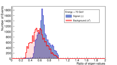
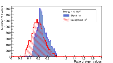
Figure 27: Distribution of $\lambda_{-}$/$\lambda_{+}$ for photons and $\pi^{0}$’s of 70 GeV for the case of fine grain information (information from individual fibers used). The plot on the left is done with linear weights for determining the impact point while the plot on the right utilizes log weights.

A comparison between the two methods using photons and $\pi^{0}$’s of 50 GeV, 70 GeV and 150 GeV indicates a higher discriminating power of the log weights. By comparing the set of plots with fine grain information in Figure 26, 27 and 28 with the corresponding plots for coarse grain information, it can be seen that not much additional sensitivity is added in the discriminating power by using information from individual fibers. Beyond 150 GeV, both the ways (coarse grain information and fine grain information) fail to discriminate between photons and $\pi^{0}$’s.

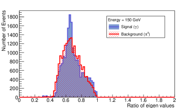
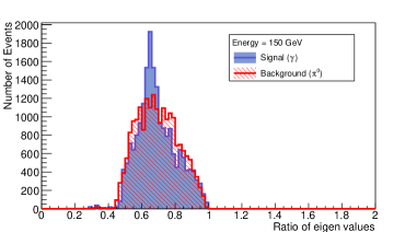
Figure 28: Distribution of $\lambda_{-}$/$\lambda_{+}$ for photons and $\pi^{0}$’s of 150 GeV for the case of fine grain information (information from individual fibers used). The plot on the left is done with linear weights for determining the impact point while the plot on the right utilizes log weights.

5.3 Study using Multivariate Analysis (MVA)

As it has been described in the previous Sections, 5.1, 5.2.1 and 5.2.2, the discriminating power is reduced significantly for $\pi^{0}$’s of energy above $100$ GeV. An analysis has been carried out exploring the discriminating power gained by employing multivariate techniques to the problem of separating $\pi^{0}$s from photons using the spatial pattern of energy deposition in the ECAL. In this analysis, the classification problem is to separate $\pi^{0}$’s from prompt photons. The following MVA classifiers are examined in this analysis:

1. Boosted Decision Tree (BDT)

2. Gradient Boosted Decision Trees (GBDT)

3. Artificial Neural Network (ANN)

In this analysis, the TMVA [15] package within ROOT [16] is used. Each MVA is trained separately on a sample of photons and $\pi^{0}$’s. Energy from each individual tower in 3$\times$3 array, or energy from each fiber in the 3$\times$3 array is fed into the MVA. This analysis is done using photons and $\pi^{0}$’s at 200 GeV. Two types of samples are produced:

Fixed gun sample:

These are produced with the gun position fixed at (0 mm, 4 cm) in $(x,y)$, with z at 3.2 m.

Random gun sample:

In this case, the gun positions are uniformly distributed both in X and Y direction between $-7$ mm and $+7$ mm i.e. within the central tower.

5.3.1 Training and testing of the MVA using fixed gun samples

The MVA is trained using 20000 events from fixed gun samples of 200 GeV photons and $\pi^{0}$’s. The following two sets of training variables are used separately to train MVA:

Coarse grain information:

Input to MVA is the ratio of energy from each tower in the 3$\times$3 array to total energy in 3$\times$3 array.

Fine grain information:

Input to MVA is the ratio of energy from each individual fiber in 3$\times$3 array to total energy in 3$\times$3 array.

These energies are scaled to the total energy collected in the 3$\times$3 array. Figure 29 shows the output response of the different MVA classifier for the case of both coarse grain and fine grain information. Figure 30 shows the background rejection versus signal efficiency curve for the case of coarse grain as well as fine grain information. It can be seen from the Figures 29 and 30, that the fine grain information is better for discriminating signal from from background.

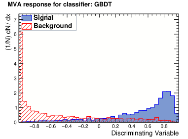
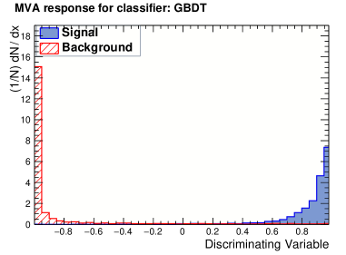
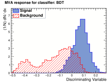
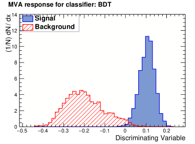
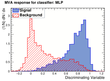
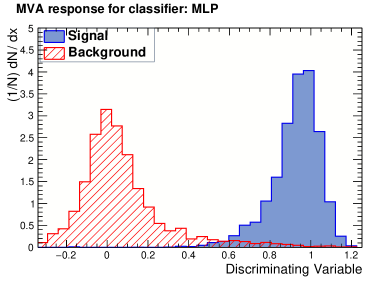
Figure 29: The output response of different MVA methods for fixed gun sample. The figures on the left are for coarse grain information and those on the right refer to fine grain information.

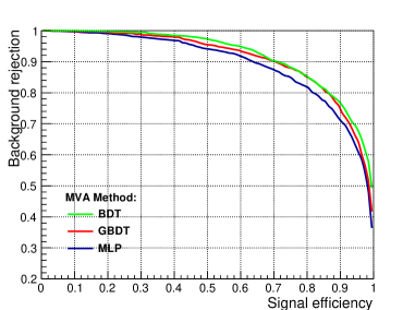
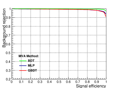
Figure 30: The background rejection versus the signal efficiency curve for various MVA methods using fixed gun sample. Left figure for coarse grain information and the figure on the right for fine grain information [17].

5.3.2 Training and testing of the MVA using random gun samples

In a realistic scenario a particle can hit anywhere on the face of a tower. Keeping this in mind a training is done on a sample of 20000 photons and $\pi^{0}$s of energy 200 GeV from random gun sources. The hit positions of the photons and $\pi^{0}$’s are uniformly distributed in X and Y direction between $-7$ mm and $+7$ mm. Two different samples are used to train the MVA:

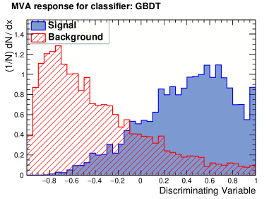
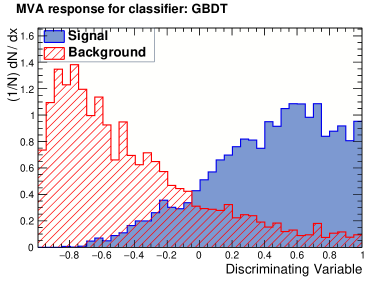
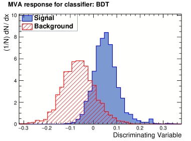
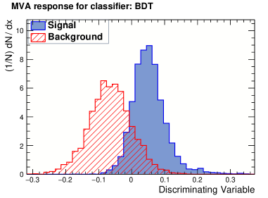
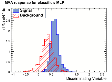
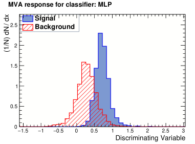
Figure 31: The output response of different MVA methods for unbinned random gun sample. The figures on the left are for coarse grain information and those on the right refer to fine grain information.

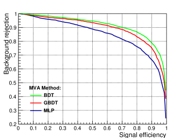
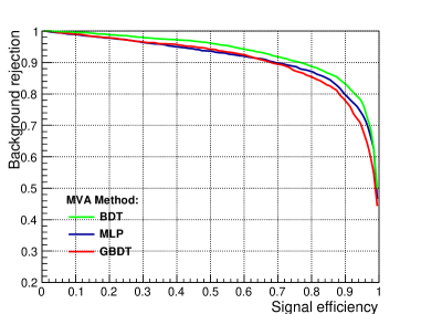
Figure 32: The background rejection versus the signal efficiency curve for various MVA methods using unbinned random gun sample. Left figure for coarse grain information and the figure on the right for fine grain information [17].

Unbinned random sample:

In this case the event sample is produced over entire face of the central tower. Figure 31 shows the output response of the different MVA classifiers for the case of both coarse grain and fine grain information. Figure 32 shows the background rejection versus signal efficiency curve for the case of coarse grain as well as fine grain information using random gun sample. It can be seen from the Figures 31 and 32, that the fine grain information improves the discrimination for the case of random gun sample also.

Binned random sample:

The energy deposit pattern in the matrix of Shashlik towers can vary considerably based on the location of the hit on the central tower. To take into account the dependence of the energy deposit pattern on the hit location, a hit location based MVA training is used, to further improve the separation power of the MVA. For this the central tower is divided into 7$\times$7 matrix of virtual square regions (or virtual cells) each of dimention 2mm$\times$2mm. Event samples are produced in each virtual cell independently. 49 separate trainings are done to obtain 49 separate trees (or networks) - one for each virtual cell. At the time of testing/using the MVA, the tree to be used is chosen using the information of the measured hit position.

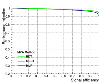
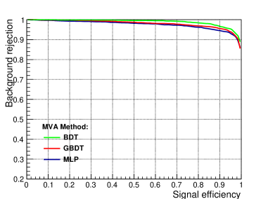
Figure 33: Background rejection versus signal efficiency of two virtual cells for the case of binned random samples. The left figure is for a virtual cell where the sample is randomized over a region from $+3$ mm to $+5$ mm in both X and Y direction and the right figure is for a region from $-1$ mm to $+1$ mm in the X direction and $+3$ mm to $+5$ mm in the Y direction with respect to the centre of the central tower [17].

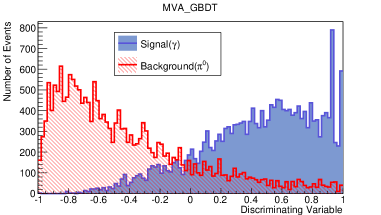
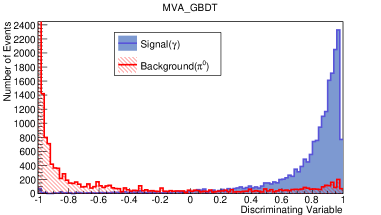
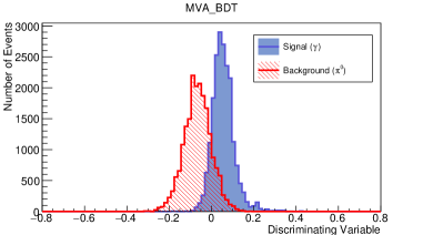
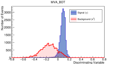
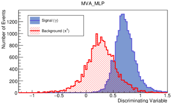
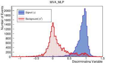
Figure 34: The output response of different MVA methods. The figures on the left show the response from the MVA trained with unbinned sample and the ones on the right are for the MVA trained with binned sample.

Figure 33 shows background rejection versus signal efficiency plots for binned random sample. Figure 34 shows the output response of both the MVA methods, namely the MVA trained with unbinned smaples and the MVAs trained with binned training samples. For both the cases, the same test sample is used.

5.4 Comparison of various methods

A comparison in performance is made among all the methods described in the previous sections. This comparison is shown for 200 GeV photons and $\pi^{0}$’s.

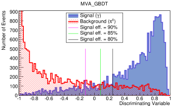
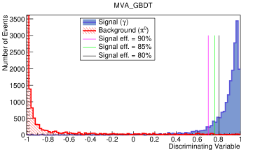
Figure 35: MVA response for 200 GeV photons and $\pi^{0}$’s. The plots on the left refers to GBDT training with coarse grain information and the plots on the right makes use of GBDT algorithm trained with fine grain information, using fixed gun sample for (x,y):(0.0 mm, 4.0 mm). The black, blue and pink lines show the point where the cut is applied to achieve 80$\%$, 85$\%$ and 90$\%$ signal efficiency (events falling on the right side of the line are selected).

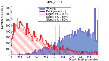
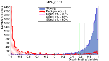
Figure 36: Comparison of GBDT MVA method for 200 GeV photons and $\pi^{0}$’s. The plots in the left refers to GBDT training with unbinned sample and the plots on the right makes use of GBDT algorithm trained with binned sample. The black, green and pink lines are the point where the cut is applied to achieve 80$\%$, 85$\%$ and 90$\%$ signal efficiency respectively [17].

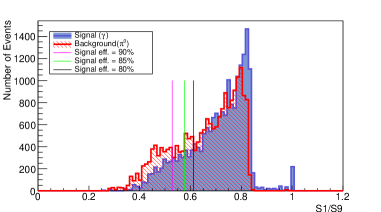
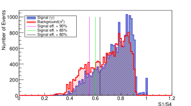
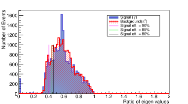
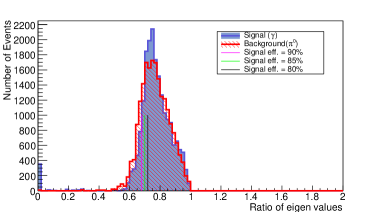
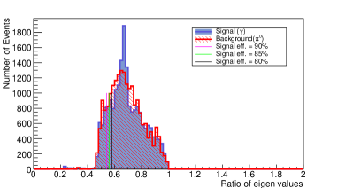
Figure 37: Distributions for 200 GeV photons and $\pi^{0}$’s of (a) $S1/S9$ on the top left; (b) $S1/S4$ on the top right; (c) ratio of eigenvalues using coarse grain information and linear weights on the middle left; (d) ratio of eigenvalues using fine grain information and linear weights on the middle right; (e) ratio of eigenvalues using coarse grain information and log weights on the bottom left; (f) ratio of eigenvalues using fine grain information and log weights on the bottom right. The black line shows the point where the cut is applied to achieve 80$\%$ signal efficiency, blue line for 85$\%$ signal efficiency and the pink line for 90$\%$ signal efficiency.

Variable	Background rejection ($\%$)
	$\epsilon_{signal}$=80$\%$	$\epsilon_{signal}$=85$\%$	$\epsilon_{signal}$=90$\%$
S1/S9	33.2	27.7	21.2
S1/S4	32.7	26.8	20.1
Linear weights: Ratio of eigenvalues (coarse grain)	21.1	15.3	9.6
Linear weights: Ratio of eigenvalues (fine grain)	23.0	18.9	12.2
Logarithmic weights: Ratio of eigenvalues (coarse grain)	41.1	36.9	32.3
Logarithmic weights: Ratio of eigenvalues (fine grain)	23.1	18.4	13.2
MVA(GBDT): coarse grain (fixed gun sample)	86.3	82.0	76.5
MVA(GBDT): fine grain (fixed gun sample)	99.1	99.0	98.5
MVA(GBDT): fine grain (unbinned random gun sample)	86.3	83.3	78.9
MVA(GBDT): fine grain (binned random gun sample)	92.3	91.0	89.3

Table 4: Table showing the background rejection for signal efficiencies of 80%, 85$\%$ and 90% for various methods. This is shown for energy point of 200 GeV [17].

If a method shows good separation power for this high energy point, then it is good for lower energy points as well.

BDT gives the best response for the case of both coarse grain and fine grain information as can be seen from the figures 30,32 and 33. The response of BDTG and BDT are similar. Here the comparison is made using the BDTG.

Table 4 shows the background rejection for all the various methods for a signal efficiencies of 80$\%$, 85$\%$ and 90$\%$.

6 Summary

A simulation study of energy and position resolution of a Shashlik detector is presented. The energy resolution is dominated by the sampling fluctuation which contributes to the stochastic term. The constant term is found to be better than 1% while the stochastic term is found to be 10.3%/$\sqrt{E}$ for light yield value of 4000 p.e./MeV. The energy resolution is found to be similar for lead/LYSO and tungsten/LYSO configurations and the optimum number of layers is found to be 28 which corresponds to $\sim$25 radiation lengths deep detector. For 125 GeV Higgs boson decaying to a pair of photon, this detector will achieve a mass resolution of 0.71 GeV when both the photons are detected in the Shashlik detector.

The position resolution using information of the Shashlik detector alone is 2.0 mm for photons of 100 GeV. The resolution improves with energy of the photon and a better resolution is obtained when the center of gravity method uses logarithmic weighting (to 0.34 mm) or a correction is made for the S-shape (to 0.22 mm).

A study of the $\pi^{0}-\gamma$ separation presented in this paper shows that the fine grain information of the shower profile collected by individual fibers is useful for separation between $\pi^{0}$ and $\gamma$ at high energies. With the MVA technique a background rejection efficiency of $90\%$ with signal efficiency $90\%$ was achieved, which is approximately three times better than the best background rejection that could be achieved by cut-based methods. We proposed a method of virtual slicing of the hit tower and impact point based training of the network, which gives an additional improvement of 8-10%. We conclude that the $\pi^{0}-\gamma$ separation power of the Shashlik calorimeter can be improved significantly by emplyoying an MVA based method with fine grain information as input and impact point based training. In this study we have considered a Shashlik detector of a specific dimension and material. However the methodology described in this paper for the resolution studies as well as the techniques employed for distinguishing between the spatial patterns of energy deposits by a photon and a $\pi^{0}$, can be easily adapted to any sampling calorimeter.

References

- [1] CMS Collaboration, The CMS experiment at the CERN LHC, JINST 3 (2008) S08004.
- [2] CMS Collaboration, Technical Proposal for the Phase-II Upgrade of the CMS detector, CERN-LHCC-2015-010 ; LHCC-P-008 (2015).
- [3] D. W. Cooke, K. J. McClellan, B. L. Bennett, J. M. Roper, M. T. Whittaker, and R. E. Muenchausen, Crystal growth and optical characterization of cerium-doped J. Appl. Phys. 88 (2000) 7360-7362.
- [4] T. Kimble, M. Chou, and B. H. T. Chai, Scintillation properties of LYSO crystals, in Proc. IEEE Nucl. Sci. Symp., 3 (2002) 1434-1437.
- [5] R.-Y. Zhu, Private communication, talk given at CMS Forward Calorimetry Meeting, CERN (2012).
- [6] S. Agostinelli, et al., GEANT4: A Simulation toolkit, Nucl. Instrum. Meth. A 506 (2003) 250.
- [7] J. B. Birks, The Efficiency of Organic Scintillators, Proc. Phys. Soc. A64 (1951) 874.
- [8] Y. Koba, et al., Scintillation efficiency of inorganic scintillators for intermediate energy charged particles, Progress in Nuclear Science and Technology 1 (2011) 218.
- [9] A. Ledovskoy, Private communication, talk given at CMS Forward Calorimetry Taskforce Meeting, CERN (2013).
- [10] F.-X. Gentit, SLitrani http://gentitfx.fr/SLitrani/.
- [11] F.-X. Gentit, Litrani: a general purpose Monte-Carlo program simulating light propagation in isotropic or anisotropic media http://gentitfx.fr/litrani/intro/intro1.html.
- [12] G. Grindhammer, S. Peters, The Parameterized Simulation of Electromagnetic Showers in Homogeneous and Sampling Calorimeters, Nucl. Instrum. Meth. A 290 (1990) 469.
- [13] Ren-yuan Zhu, Crystal calorimeters in the next decade, Physics Procedia, 37 (2012) 372-383.
- [14] R.-Y. Zhu, Private communication, talk given at CMS Forward Calorimetry Taskforce Meeting, CERN (2012).
- [15] A. Hoecker, et al., Tmva toolkit for multivariate data analysis with root, http://tmva.sourceforge.net/ (2013).
- [16] Root, http://root.cern.ch/drupal/.
- [17] A. Roy, Sh. Jain, S. Banerjee, S. Bhattacharya and G. Majumder, Simulation of Separation Study for Proposed CMS Forward Electromagnetic Calorimeter, Journal of Physics: Conference Series 759 (2016) 012074.