Supernova-regulated ISM – V. Space- and time-correlations

Abstract

We apply correlation analysis to random fields in numerical simulations of the supernova-driven interstellar medium (ISM) with the magnetic field produced by dynamo action. We solve the thermo-magnetohydrodynamic (MHD) equations in a shearing, Cartesian box representing a local region of the ISM, subject to thermal and kinetic energy injection by supernova explosions, and parameterized optically-thin radiative cooling. We consider the cold, warm  and hot phases of the ISM separately; the analysis mostly considers the warm gas, which occupies the bulk of the domain. Various physical variables have different correlation lengths in the warm phase: $40\,{\rm pc}$, $50\,{\rm pc}$, and $60\,{\rm pc}$ for random magnetic field, density, and velocity, respectively, in the midplane. The correlation time of the random velocity is comparable to the eddy turnover time, about $10^{7}\,{\rm yr}$, although it may be shorter in regions with higher star formation rate. The random magnetic field is anisotropic, with the standard deviations of its components $b_{x}/b_{y}/b_{z}$ having approximate ratios $0.5/0.6/0.6$ in the midplane. The anisotropy is attributed to the global velocity shear from galactic differential rotation, and locally inhomogeneous outflow to the galactic halo. The correlation length of Faraday depth along the $z$-axis, $120\,{\rm pc}$, is greater than for electron density, $60\text{--}90\,{\rm pc}$, and vertical magnetic field, $60\,{\rm pc}$. Such comparisons may be sensitive to the orientation of the line of sight. Uncertainties of the structure functions of synchrotron intensity rapidly increase with the scale. This feature is hidden in power spectrum analysis, which can undermine the usefulness of power spectra for detailed studies of interstellar turbulence.

1. Introduction

The interstellar medium (ISM) of a spiral galaxy is a complex, multiphase, random system, driven by the input of thermal and kinetic energy from supernova (SN) explosions and stellar winds (e.g., Mac Low & Klessen, 2004; Elmegreen & Scalo, 2004; Scalo & Elmegreen, 2004; Mac Low et al., 2005; de Avillez & Breitschwerdt, 2005; Federrath et al., 2010; Hill et al., 2012). Its statistical analysis, including that of interstellar turbulence, is complicated by the multi-phase structure, where the diversity of physical processes predominant in different phases causes strong inhomogeneity. Furthermore, interstellar turbulence is transonic or supersonic (Bykov & Toptygin, 1987; Vázquez-Semadeni, 2015). The compressibility and abundance of random shock waves lead to spatial and temporal intermittency of the random velocity and magnetic fields and of the density fluctuations. Dynamo action adds further complexity by producing intermittent random magnetic fields (Wilkin et al., 2007).

Observational studies of such an inhomogeneous, complex random system are severely limited by the fact that observable quantities are integrals along the line-of-sight, so that many physically significant statistical features become hidden. When observed at a low resolution, the interstellar medium can be satisfactorily described in terms of Gaussian random fields, but recent observations have revealed a plethora of density structures in neutral hydrogen, mostly planar or filamentary (Heiles & Troland, 2003; Makarenko et al., 2015; Wang et al., 2016, and references therein). Statistical analysis of such random fields cannot be restricted to the standard tools of the theory of Gaussian random functions (and related ones, such as log-normal and $\chi^{2}$ functions), where the probability distribution and second-order correlation functions provide a complete description. However, correlation analysis remains an important first step, where the form of the correlation function, the correlation length (or time) and the mean-square variations of a variable are the most important quantities explored.

There are numerous and diverse estimates of the integral (correlation) scale of interstellar turbulence $l_{0}$ (see also Haverkorn & Spangler, 2013). The autocorrelation function of the line-of-sight H I cloud velocities obtained in the Milky Way by Kaplan (1966) leads to $l_{0}\simeq 80\,{\rm pc}$. Lazaryan & Shutenkov (1990) found $l_{0}\approx 50\,{\rm pc}$ from the fluctuations in synchrotron intensity. Ohno & Shibata (1993) used differences in Faraday rotation between neighboring pulsars to obtain $10<l_{0}<100\,{\rm pc}$. Minter & Spangler (1996) yielded $l_{0}\simeq 4\,{\rm pc}$ from the structure functions of the variations in the Faraday rotation and emission measures across extended extragalactic radio sources. Structure functions of the Faraday rotation of extragalactic sources (Haverkorn et al., 2004, 2006, 2008) and their degree of depolarization (Haverkorn et al., 2008) give $l_{0}\simeq 1\,{\rm pc}$ in the Milky Way’s spiral arms. $l_{0}<20\,{\rm pc}$ was found by an analysis of low-frequency synchrotron intensity fluctuations from a large region of the Galactic disk by Iacobelli et al. (2013). In the Large Magellanic Cloud, the structure function of the Faraday rotation of more distant sources gave $l_{0}\simeq 90\,{\rm pc}$ (Gaensler et al., 2005). In the galaxy M51 Fletcher et al. (2011) obtained $l_{0}\simeq 50\,{\rm pc}$ from the depolarization of diffuse emission, whilst Houde et al. (2013) found $l_{0}\simeq 65\,{\rm pc}$ from the dispersion of radio polarization angles. These estimates are strikingly different, perhaps not surprisingly. They have been obtained from diverse tracers, and it is not surprising that the correlation length of the gas velocities, Faraday rotation measure and synchrotron fluctuations differ (the latter being nonlinear functions of the fluctuating quantities). A relation between the correlation length of the product of random functions and those of the multipliers depends on their detailed statistical properties (e.g., §6.2 in Stepanov et al., 2014). Our aim here is to clarify this relation. This would be difficult to do with observational data, at least at present.

Interpretations of observations of polarized synchrotron emission and its Faraday rotation suggest that a significant fraction of the polarization may be due to anisotropy of the random magnetic field. The correlation between the mean Faraday rotation and its standard deviation along the Galactic disc, found by Brown & Taylor (2001), was the earliest indication of an anisotropic random field. Subsequent models of various components of Milky Way emission along the Galactic disk (Jaffe et al., 2010, 2011, 2013) and across the entire sky (Jansson & Farrar, 2012a, b) required the inclusion of an anisotropic random magnetic field in order to fit the observations. In other galaxies, modeling of pre- and post-shock polarized emission in the barred galaxies NGC1097 and NGC1365 (Beck et al., 2005) and the spiral galaxy M51 (Fletcher et al., 2011), the dispersion of polarization angles in M51 (Houde et al., 2013), comparison of the observed polarized emission and Faraday rotation in M33 (Stepanov et al., 2014), and modeling depolarization in M51 (Shneider et al., 2014), have all indicated the presence of anisotropic random fields. Extracting the degree of anisotropy from the observations, though, is difficult.

In M51, Fletcher et al. (2011) estimate that the ratio of the standard deviations of the random magnetic field components in orthogonal directions is $\sigma_{x}/\sigma_{y}\simeq 2$ and Houde et al. (2013) obtained a ratio of correlation lengths along and perpendicular to the local mean-field direction of $l_{\parallel}/l_{\perp}\simeq 1.8$. As with observational estimates for $l_{0}$, it is appropriate to carefully examine the possible anisotropy of the random magnetic field.

Simulations of the SN-regulated ISM have become sufficiently realistic to treat them as numerical experiments. It is then natural to use sufficiently realistic numerical models to address these questions before the more difficult observational exploration. We use such simulations, as detailed in Gent (2012) and Gent et al. (2013a, b), which have non-trivial magnetic fields generated by dynamo action, to clarify the correlation (and other statistical) properties of the multi-phase ISM. In particular, we compare the autocorrelation and cross-correlation functions of the random (i.e., small-scale; see §2.3) velocity and magnetic fields and density fluctuations, as well as the Faraday depth and synchrotron intensity.

However complex, the simulations of the ISM can hardly be considered as trustworthy representations of the ISM in its whole complexity. Therefore, the goal of our analysis is not to achieve quantitative agreement with observations in every detail (although the general agreement is quite remarkable) but rather to identify those physical processes that shape the simulated ISM and are likely to be important in reality.

Turbulent flows are often represented in spectral space, in terms of the Fourier transforms of the physical variables. Such transforms are straightforward in infinite or periodic spaces. However, simulations of the ISM are performed in relatively small domains, only containing of order one thousand correlation cells, not simply-periodic because of the open (or similar) boundary conditions at the top and bottom of the domain, and statistically inhomogeneous because of the stratification (e.g. Korpi et al., 1999b, a; Gent et al., 2013a). Furthermore, it is difficult to estimate reliably the statistical uncertainty of the Fourier transforms.

We therefore proceed via correlation analysis (e.g., Monin & Yaglom, 1975). For most of the work, we assume local isotropy in the horizontal ($xy$) plane; this assumption is assessed in §5.

Correlation lengths obtained from comprehensive numerical simulations of the multi-phase ISM exhibit less diversity than the observational results. Joung & Mac Low (2006) obtain a gas density spectrum with a peak at $20\,{\rm pc}$, whereas most kinetic energy is contained at scales $20\text{--}40\,{\rm pc}$. Gent et al. (2013a) calculate $l_{0}=100\,{\rm pc}$ for the random velocity field in the mid-plane of the galaxy, also from hydrodynamic simulations. In the MHD simulations of de Avillez & Breitschwerdt (2007), $l_{0}=70\,{\rm pc}$ for the random velocity field. This scale fluctuates strongly with time. From correlation analysis of the vertical component of random velocity, Korpi et al. (1999b) obtained an estimate of $l_{0}=30\,{\rm pc}$ for the warm gas at all heights, whereas in the hot gas $l_{0}$ increases from $20\,{\rm pc}$ in the mid-plane to $60\,{\rm pc}$ at $|z|=150\,{\rm pc}$.

The paper is organized as follows. The simulations of the SN-driven ISM and averaging procedure used in our analysis are presented in §2. The spatial correlations of the random magnetic field, density and velocity are discussed in §3, whereas time correlations are the subject of §4. The anisotropy of the random magnetic field in the simulated ISM is estimated and interpreted in §5. The autocorrelation functions of such observable quantities as the Faraday depth and synchrotron intensity are obtained and discussed in §6. Our results are summarized in §7. Appendix A presents a comparison with the results obtained in a larger computational domain.

2. Simulations of the multi-phase ISM

We use our earlier simulations of the ISM based on the Pencil Code (https://github.com/pencil-code), using its ISM modules that implement SN energy injection and radiative cooling, and handle shocks produced in a supersonic flow, described in detail by Gent (2012) and Gent et al. (2013a).

The simulations involve solving the full, compressible, non-ideal MHD equations with parameters generally typical of the solar neighborhood in a three-dimensional local Cartesian, shearing box with radial ($x$) and azimuthal ($y$) extents of $L_{x}=L_{y}=1.024\,{\rm kpc}$ and vertical ($z$) extent $L_{z}=1.086\,{\rm kpc}$ on either side of the mid-plane at $z=0$.

Our numerical resolution is $\Delta x=\Delta y=\Delta z=4\,{\rm pc}$, using $256$ grid points in $x$ and $y$ and $544$ in $z$. Gent et al. (2013a) demonstrate that this resolution is sufficient to reproduce the known solutions for expanding SN remnants in the Sedov–Taylor and momentum-conserving phases.

Details of the numerical implementation and its comparison with other similar simulations can be found in Section 2.1.

The basic equations are mass conservation, the Navier–Stokes equation, the heat equation, and the induction equation, solved for mass density $\rho$, velocity $\bm{u}$, specific entropy $s$, and magnetic vector potential $\bm{A}$ (such that $\bm{B}=\nabla\times\bm{A}$).

The Navier–Stokes equation includes a fixed vertical gravity force that includes contributions from the stellar disk and spherical dark halo. The initial state is an approximate hydrostatic equilibrium. The Galactic differential rotation is modelled by a background shear flow $\bm{U}=(0,-q\Omega x,0)$, where $q$ is the shear parameter and $\Omega$ is the Galactic angular velocity. Here we use $q=\bm{+1}$, as in a flat rotation curve, and $\Omega=25\,{\rm km\,s^{-1}}\,{\rm kpc}^{-1}$, as in the Solar neighborhood.

The velocity $\bm{u}$ is the perturbation velocity in the rotating frame, that remains after the subtraction of the background shear flow from the total velocity. However, it still contains a large-scale vertical component due to an utflow driven by the SN activity.

Both Type II and Type I SNe are included in the simulations. These differ in their vertical distribution and frequency only. The frequencies used correspond to those in the Solar neighborhood. We introduce Type II SNe at a mean rate, per unit surface area, of $\nu_{\rm II}=25\,{\rm kpc}^{-2}\,{\rm Myr}^{-1}$. Type I SNe have a mean rate, per unit surface area, of $\nu_{\rm I}=4\,{\rm kpc}^{-2}\,{\rm Myr}^{-1}$.

The SN sites are distributed randomly in the horizontal planes. Their vertical positions have Gaussian distributions with scale heights of $h_{\rm II}=0.09\,{\rm kpc}$ and $h_{\rm I}=0.325\,{\rm kpc}$ for SNII and SNI, respectively. No spatial clustering of the SNe is included. The thermal energy injected with each SN is $0.5\times 10^{51}\,{\rm erg}$. Injected velocity and the uneven density within each explosion site randomly adds kinetic energy with mean $0.4\times 10^{51}\,{\rm erg}$.

We include radiative cooling with a parameterized cooling function. For $T<10^{5}\,{\rm K}$, we adopt a power-law fit to the ‘standard equilibrium’ pressure–density curve of Wolfire et al. (1995), as given in Sánchez-Salcedo et al. (2002). For $T>10^{5}\,{\rm K}$, we use the cooling function of Sarazin & White (1987). This cooling allows the ISM to separate into distinct hot, warm and cold phases identifiable as peaks in the joint probability distribution of gas in density and temperature.

Photoelectric heating is also included as in Wolfire et al. (1995). The heating decreases with $|z|$ on a length scale comparable to the scale height of the disk near the Sun.

Shock-capturing kinetic, thermal and magnetic diffusivities (in addition to constant small background diffusivities), are included to resolve shock discontinuities and maintain numerical stability in the Navier–Stokes, heat and induction equations.

Periodic boundary conditions are used in $y$, and sheared-periodic boundary conditions in $x$ (considered in more detail in §2.5). Open boundary conditions, permitting outflow and inflow, are used at the vertical ($z$) boundaries. See Gent (2012) and Gent et al. (2013a, b) for further details on the boundary conditions used and on the other implementations described above.

Starting with a weak initial azimuthal magnetic field at the mid-plane, this system is susceptible to the dynamo instability. Dynamo action can be identified (Gent et al., 2013a) with exponential field growth saturating after $1.4\,{\rm Gyr}$, at root mean square field strengths of order $2.5\,\mu{\rm G}$, comparable to observational estimates for the solar neighbourhood.

Our analysis is based on 12 snapshots of the computational volume in the range $1.4\leq t\leq 1.675\,{\rm Gyr}$, by which time the system, including the large-scale magnetic field, has reached a statistically steady state. The interval between the snapshots, $25\,{\rm Myr}$, is significantly longer than the correlation time of the random flow (see §4), and is sufficient for the snapshots to be considered statistically independent.

To test the influence of shear rate on the correlations, we also analyse data from a model with twice the rotation rate, as discussed in Gent et al. (2013b). We use $12$ snapshots in the range $1.4\leq t\leq 1.675\,{\rm Gyr}$, again with a separation of $25\,{\rm Myr}$, with the magnetic field saturated as for the main run. Any notable differences between the results for the different models will be reported throughout the text.

2.1. Parameters of the numerical model

The model discussed here aims to reproduce the statistical properties of the random ISM. With the integral scale of random fluctuations in various physical variables of order $50\,{\rm pc}$ (see below), the computational domain that we use contains about $400$ correlation cells, providing sufficient statistics to obtain useful results. Other simulations of comparable physical content (Hill et al., 2012; Bendre et al., 2015) have computational boxes of a similar horizontal size of $0.8\text{--}1\,{\rm kpc}$. Physically distinct objects of the next largest scale are superbubbles, of order $0.5\text{--}1\,{\rm kpc}$ in size, and OB associations and spiral arms whose scale is of order $1\text{--}3\,{\rm kpc}$; modelling these phenomena would require significantly larger computational domains (and the next generation of computational models) although some of their features can be captured with existing models (e.g., Shukurov et al., 2004; de Avillez & Breitschwerdt, 2007).

The size of the superbubbles produced by SNe clustering are comparable to the horizontal size of the computational domain. As a result, we neglect the clustering of SNe, although it would not be difficult to include it. Simulations in a domain of a significantly larger size are required to capture the effects of the SN clustering. de Avillez & Breitschwerdt (2007) include SN clustering in their simulations and obtain the correlation scale of the random flows of $\bm{75}\,{\rm pc}$, comparable to those obtained below. In order to fully understand the effects of clustering, simulations without clustering must first be understood, which is the purpose of the current work.

The vertical size of the domain is largely controlled by its horizontal size. A vertical extent of $1\,{\rm kpc}$ is insufficient to capture fountain flows and model the temperature distribution in the halo, which require heights of greater than $5\,{\rm kpc}$ (see Hill et al., 2012). However, our simulations are able to fulfil our purpose of capturing the physics of the ISM near the midplane, excluding fountain flows, without any effects introduced via periodic boundary conditions. As argued by Gent et al. (2013a), periodic boundary conditions in the horizontal planes affect the outflow speed significantly at altitudes exceeding the horizontal extent of the region. Furthermore, the diameter of supernova shells increases to $0.4\text{--}0.6\,{\rm kpc}$ at $|z|\simeq 1\,{\rm kpc}$. Therefore, results obtained at $|z|\gtrsim 1\,{\rm kpc}$ in a computational box of $1\times 1\,{\rm kpc}^{2}$ horizontally may be questionable. Results from recent simulations performed in computational boxes taller than $1\,{\rm kpc}$ are mostly reported only within a few kiloparsecs from the midplane (e.g., Hill et al., 2012). The domain used in our simulations includes two scale heights of the warm neutral gas.

With the range of $|z|$ limited to $1\,{\rm kpc}$ in our simulations, we have paid special effort to ensuring that the boundary conditions at the top and bottom boundaries do not introduce any apparent artefacts into numerical solutions, such as a boundary layer with a strong gradient in any of the physical variables (Appendix C of Gent et al., 2013a). The limited vertical extent of the box is the main limitation of our model, but it can only be increased together with its horizontal size. Appendix A presents results obtained with a slightly larger domain (three times the volume of the domain used for the main computations). We conclude that the results reported here are not affected by the change in the simulated volume.

The mass loss rate through the top and bottom boundaries is about $10^{-3}\,{\rm M_{\sun}}\,{\rm yr}^{-1}$, so $10^{6}\,{\rm M_{\sun}}$ is lost in $1\,{\rm Gyr}$, as compared to the total gas mass of $10^{7}\,{\rm M_{\sun}}$ in the computational domain. This mass loss would correspond to a total mass loss rate of $1\,{\rm M_{\sun}}\,{\rm yr}^{-1}$ for a galactic disk of radius $15\,{\rm kpc}$, assuming the Galaxy is in a steady state. Our open boundary conditions allow for inflow as well as outflow (albeit in a rather ad hoc way), which mitigates mass loss through the boundaries. The mass loss, albeit only modest, was compensated by a continuous mass replenishment (in proportion to the local gas density, for minimal impact on the dynamics) to maintain an approximately constant gas mass throughout the simulations.

The numerical resolution of $4\,{\rm pc}$ that we use has been carefully selected to reproduce accurately the known expansion laws and approximate internal structure of an isolated supernova remnant, subject to radiative cooling processes, until its radial shell expansion slows to match the ambient adiabatic speed of sound (Appendix B of Gent et al., 2013a). Thus, we are confident that our simulations model reliably the associated energy injection into the diffuse ISM. Indeed, the intensity of random flows, of order $10\,{\rm km\,s^{-1}}$ in the warm gas and higher in the hot phase, is in full agreement with both observations and simulations at a higher resolution. This is also true of the scales of the random flows, fractional volumes of the ISM phases and other aspects of the modelled ISM. We have adjusted thermal conductivity so as to ensure that any structures produced by thermal instability are fully resolved at the $4\,{\rm pc}$ resolution. Comparable simulations of de Avillez & Breitschwerdt (2007); de Avillez & Breitschwerdt (2012a) have an adaptive mesh with the finest separation of $1.25\,{\rm pc}$, whereas Hill et al. (2012) have a resolution of $2\,{\rm pc}$, both representing an arguably modest improvement. We were unable to identify any differences in the relevant results of all these simulations that might be a consequence of the difference in numerical resolution. We also note that adaptive mesh refinement makes it difficult to include differential rotation, a crucial element of realistic modelling of magnetic field.

Self-gravity is ignored in our simulations since we do not attempt to model the very cold molecular gas which is significantly affected by self-gravity. Simulations with higher resolution would be required to model the higher densities and the associated cooling rates.

2.2. The multi-phase structure

The numerical model exhibits three distinct states of the gas corresponding to local maxima in the probability distribution function (PDF) of the specific entropy $s$. Gas parameters in those states are similar to the three main phases of the ISM. Following Gent et al. (2013a), the cold phase is defined as that having $s\leq 3.7\times 10^{8}\,{\rm erg}\,{\rm K}^{-1}$, the hot phase has $s\geq 23.2\times 10^{8}\,{\rm erg}\,{\rm K}^{-1}$, with the warm phase in between. The three phases have very different physical properties, including the random velocity and magnetic fields, as well as differing in their mean temperature and density. Therefore, our analysis is carried out for each phase separately. For this purpose, only grid points corresponding to a given phase are retained in the data cubes containing each physical variable, with the other points masked out. This allows us to do the averaging required in the computation of the structure functions over disjoint regions in the physical space.

Figure 1.— Aligned domains of logarithm of gas number density (${\log n}$), at $z=2\,{\rm pc},\,t=1.55\,{\rm Gyr}$; (a) before and (b) after shifting the right-hand domain by $\delta y$ to account for the shearing boundary. The boundary between the two copies of the computational domain is here located at $x=0$.

2.3. Averaging procedure

Our analysis is conducted for the moduli of the random magnetic and velocity fields and the gas density fluctuations, denoted $b$, $u^{\prime}$ and $n^{\prime}$, respectively. The random velocity $\bm{u}^{\prime}$ should be carefully distinguished from the velocity perturbation $\bm{u}$, defined as the deviation from the background large-scale shear flow, since the latter contains a systematic vertical velocity.

Since the mean vertical velocity and the large-scale magnetic field are not necessarily uniform across any horizontal plane, we do not use horizontal averages to define the mean magnetic field as is often done in the literature, but instead follow Gent et al. (2013b) and use Gaussian smoothing, within the framework of Germano (1992). The mean (large-scale) component of a random field $f$, averaged over a scale $\ell$ and denoted $\langle f\rangle_{\ell}$, is defined by a convolution with a Gaussian kernel $G_{\ell}(\bm{x})$,

$$\langle f\rangle_{\ell}(\bm{x})=\int_{V}f(\bm{x}^{\prime})\,G_{\ell}(\bm{x}-\bm{x}^{\prime})\,\mathrm{d}^{3}\bm{x}^{\prime},$$

$$G_{\ell}(\bm{x})=(2\pi\ell^{2})^{-3/2}\exp[-\bm{x}^{2}/(2\ell^{2})]\,,$$ (1)

where integration is extended to the volume occupied by a given ISM phase or the total volume as appropriate. The random velocity is then $\bm{u}^{\prime}=\bm{u}-\langle\bm{u}\rangle_{\ell}$ and similarly for the magnetic field, $\bm{b}=\bm{B}-\langle\bm{B}\rangle_{\ell}$ and the gas number density, $n^{\prime}=n-\langle n\rangle_{\ell}$. Following Gent et al. (2013b), we use $\ell=50\,{\rm pc}$.

As discussed by Gent et al. (2013b), a significant fraction of the energy in the random field remains at length scales greater than $\ell$. To clarify the consequences of this, consider averaging a random field $f(\bm{x})$ in wave number ($\bm{k}$) space, denoting $\widehat{f}(\bm{k})$ the Fourier transform of $f(\bm{x})$. By the convolution theorem, the mean field $\langle f\rangle_{\ell}(\bm{x})$ has the Fourier transform $\langle\widehat{f}\rangle_{\ell}(\bm{k})=\widehat{f}(\bm{k})\,\widehat{G}_{\ell}(\bm{k})$, where $\widehat{G}_{\ell}(\bm{k})$ is the transform of the smoothing kernel. For the Gaussian kernel $G_{\ell}(\bm{x})$, we have $\widehat{G}_{\ell}(\bm{k})=\exp(-\ell^{2}\bm{k}^{2}/2)$, so $\langle\widehat{f}\rangle_{\ell}(\bm{k})=\exp(-\ell^{2}\bm{k}^{2}/2)\widehat{f}(\bm{k})$. Thus, for variations with wavenumber $k$ (and wavelength $\lambda=2\pi/k$), a fraction $\exp(-\ell^{2}\bm{k}^{2})$ of the original field energy is interpreted as that of the mean field, and the remainder goes into the random field. This fraction is half – i.e., the field energy is equally split between mean and random fields – at the wave number $k_{\rm eq}=\sqrt{\ln 2}/\ell$, or the wavelength $\lambda_{\mathrm{eq}}=2\pi\ell/\sqrt{\ln 2}\approx 7.5\ell$. Thus, with $\ell=50\,{\rm pc}$, the field energy is equally split at the wavelength $\lambda_{\rm eq}\approx 380\,{\rm pc}$ between the mean and random parts. Variations with wavelength $\lambda<380\,{\rm pc}$ go predominantly into the random field, and increasingly so as $\lambda$ decreases; for features with $\lambda=50\,{\rm pc}$, only a fraction $\exp(-4\pi^{2})\approx 10^{-17}$ of the energy goes into the mean field.

2.4. The structure and correlation functions

We start the calculations with the second-order structure functions $D(l)$, which are more robust than the correlation functions, $C(l)$, with respect to errors (§13.1 in Monin & Yaglom, 1975):

$$D(l)=\langle[f(\bm{x}+\bm{l})-f(\bm{x})]^{2}\rangle_{l},$$ (2)

where $\bm{x}$ a given position in the $(x,y)$-plane and $\bm{l}$ a horizontal offset with $l=|\bm{l}|$. Analysis is restricted to horizontal planes with no offsets in the $z$-direction, because of the stratification in $z$.

Since we are dealing with periodic (or sheared periodic) functions in $x$ and $y$, the maximum offsets we can consider in the $x$ and $y$ directions are half the domain sizes in each direction. Hence, we consider offsets in the range $0\leq l_{x}\leq L_{x}/2,\,0\leq l_{y}\leq L_{y}/2$. Using $D(l)$, the autocorrelation function $C(l)$ is obtained as

$$C(l)=1-\frac{D(l)}{2\sigma^{2}},$$ (3)

where $2\sigma^{2}$ is the value of $D(l)$ at which the random function $f(\bm{x})$ is no longer correlated, and $\sigma$ is the dispersion (r.m.s. value) of $f(\bm{x})$. The choice of $2\sigma^{2}$ in a finite domain is not always obvious (see below). In terms of $C(l)$, the correlation length $l_{0}$ is defined as

$$l_{0}=\int_{0}^{\infty}C(l)\,\mathrm{d}l.$$ (4)

The magnitude of the implied correlation length is very sensitive to the range of integration and to the behaviour of the correlation function at large $l$. An exponentially small tail in $C(l)$ can make a significant contribution to $l_{0}$.

To address this problem, we fit the structure functions obtained from equation (2) to one of the following analytic forms (as discussed below), thereby obtaining estimates of $\sigma^{2}$ and $L_{0}$ (and hence $l_{0}$):

$$D(l) =2\sigma^{2}\left[1-\exp\left(-\frac{l}{L_{0}}\right)\right],\qquad l_{0}=L_{0},$$ (5)

$$D(l) =2\sigma^{2}\left[1-\exp\left(-\frac{l^{2}}{2L_{0}^{2}}\right)\right],\qquad l_{0}=\sqrt{\frac{\pi}{2}}\,L_{0}.$$ (6)

Since the governing equations contain second-order derivatives in spatial coordinates, the spatial variations must be smooth random functions of position, so that $\mathrm{d}C/\mathrm{d}l=0$ at $l=0$ for spatial correlations. However, the fact that only the first time derivatives appear in the governing equations implies that the time variations only needs to be continuous, so that $\mathrm{d}C/\mathrm{d}\tau\neq 0$ for $\tau=0$ may be expected for time correlations (as considered in §4), with $\tau$ the time lag.

We indeed observe this difference in the computed structure and correlation functions, and use form in equation (5) for time correlations and equation (6) for spatial correlations. Some of the spatial autocorrelation functions discussed below (most notably those for the density fluctuations) exhibit an oscillatory behavior; in such cases, equation (6) is augmented to

$$D(l)=2\sigma^{2}\left[1-\exp\left(-\frac{l^{2}}{2L_{0}^{2}}\right)\cos(kl)\right],$$ (7)

with $k=al+b$, where $a$ and $b$ are two additional parameters determined by the zeros in the correlation function.

The correlation lengths $l_{0}$ are presented in Table 1. To confirm the importance of using fitted correlation functions, we also present in this table the correlation lengths $\tilde{l}_{0}$ obtained by integration of the directly calculated $C(l)$, over the range $0\leq l\leq 500\,{\rm pc}$. The values differ by up to a factor of $2$, with the differences being greatest for density fluctuations (where the form in equation (7) was used); the agreement for random magnetic field and velocity (where the form in equation (6) was used) is closer.

To improve the reliability of our statistics, the averaging involved in the calculation of the structure functions is performed over 26 grid planes within layers at $|z|\leq 50\,{\rm pc}$, $|z-0.4\,{\rm kpc}|\leq 50\,{\rm pc}$ and $|z+0.4\,{\rm kpc}|\leq 50\,{\rm pc}$ for each snapshot, and then the structure functions are further averaged over the snapshots. The uncertainty of the resulting values of the structure functions is rather small (of order $10^{-3}$ in terms of the relative error) because of the large number of data-point pairs available even at large values of $l$. The structure and correlation functions in figures below are shown with error bars representing not their uncertainty but the standard deviation of the individual measurements around the mean.

Table 1 The root-mean-square (rms) values of the fluctuations, their magnitude relative to the mean and correlation lengths of the fluctuations in gas density, speed and magnetic field for the warm gas at the mid-plane $z=0$ and at $|z|=400\,{\rm pc}$.

$|z|$	Density fluctuations					Random speed					Random magnetic field
	rms	rms	$l_{0}$	$\tilde{l}_{0}$		rms	rms	$l_{0}$	$\tilde{l}_{0}$		rms	rms	$l_{0}$	$\tilde{l}_{0}$
$[\text{pc}]$	[cm-3]	relative	[pc]	[pc]		[km/s]	relative	[pc]	[pc]		$[\mu$G]	relative	[pc]	[pc]
0	$0.306\pm 0.001$	$0.49\pm 0.03$	$53\pm 5$	$24\pm 1$		$8.10\pm 0.03$	$1.0\pm 0.1$	$60\pm 3$	$50\pm 1$		$0.587\pm 0.002$	$0.58\pm 0.04$	$44\pm 2$	$41\pm 1$
400	$0.0604\pm 0.0001$	$0.49\pm 0.03$	$37\pm 2$	$27\pm 2$		$2.84\pm 0.01$	$0.49\pm 0.11$	$87\pm 3$	$81\pm 1$		$0.483\pm 0.001$	$0.39\pm 0.05$	$64\pm 2$	$55\pm 1$

Figure 2.— (a) The structure function $D(l)$ and (b) correlation functions $C(l)$ for density fluctuations in the warm gas, averaged about $z=-400\,{\rm pc}$ (blue, dashed), $z=0\,{\rm pc}$ (black, solid), and $z=400\,{\rm pc}$ (red, dash-dotted). The error bars denote the standard deviation of the individual measurements around their mean values, rather than the error of the mean value, as discussed in §2.4. For clarity, the error bars are only shown for every sixth bin in $l$, and staggered between the different curves.

2.5. Accounting for shearing boundaries

When calculating the increments in the structure function, we use pairs of points separated by the periodic boundaries in $x$ and $y$. In the shearing box, the horizontal periodicity conditions (see Hawley et al., 1995) for a variable $f$ are

$$f(x,y,z) =f(x+L_{x},y-\delta y(t),z)\quad (\text{boundary in }x),$$ (8)

$$f(x,y,z) =f(x,y+L_{y},z) (\text{boundary in }y),$$

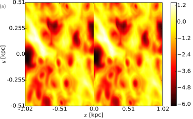
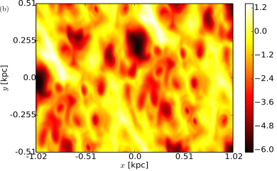
where $\delta y(t)=\mathrm{mod}[q\Omega L_{x}t,L_{y}]$ is the time-varying offset between the shearing boundaries in $x$ (mapped to the range $0\leq\delta y<L_{y}$). In order to conveniently include pairs of points located on different sides of the periodic boundary in $x$, we extend the computational domain in the $x$-direction by its copy and shift it by $\delta y(t)$ to remove the discontinuity between the two domains, as shown in Figure 1.

3. Spatial correlations

Figure 3.— As in Fig. 2, but for the random speed in the warm gas.

Figure 4.— As in Fig. 2, but for the modulus of the random magnetic field in the warm gas.

As described above, we calculate the spatial structure- and correlation-functions for the random magnetic and velocity fields and the fluctuations in the gas number density separately for the warm and hot gas. The correlation functions are then used to estimate the correlation lengths of these variables. Spatial correlations of the Faraday depth and synchrotron emissivity are discussed in §6.

The results are shown in Table 1 and Figure 2 for the density fluctuations, Figure 3 for the random speed and Figure 4 for the magnitude of the random magnetic field. The structure functions used to obtain the autocorrelation functions are only shown in Figure 2a: those for the other variables have a similar form. The magnitudes of the fluctuations in the variables and their correlations lengths are discussed in the next two sections.

The uncertainties of the root-mean-square (rms) values of various variables and their correlations lengths given in Tables 1, 2 and 5 have been obtained as 95% confidence intervals from weighted least-squares fitting of equation (6), or for the gas density equation (7). The weights used are the uncertainties of the values of the correlation function rather than the standard deviations shown in the figures.

The uncertainties in the rms values and correlation lengths thus obtained are underestimates of the true uncertainty as they do not take into account any systematics errors, such as those arising from the uncertain value of the computed structure functions at $l\to\infty$.

3.1. Magnitude of the fluctuations

The rms magnitudes of the fluctuations are shown in Table 1, together with the rms values of the relative fluctuations, $\langle(f^{\prime}/\langle f\rangle_{l})^{2}\rangle^{1/2}$ for a variable $f$; we stress that the mean value $\langle f\rangle_{l}$ is a function of position. In the case of velocity fluctuations, the average velocity, $\langle\bm{u}\rangle_{l}=0$, refers to the sheared frame, that is, includes the systematic outflow velocity, but not the overall rotation or the shear due to the galactic differential rotation.

In each phase, the standard deviation of the density fluctuations decreases with $|z|$ together with the average density. The relative magnitude of the fluctuations also decreases, but more slowly.

As shown in Fig. 2, density fluctuations are weakly anti-correlated in the range of scales $80\leq l\leq 250\,{\rm pc}$ at each height, with the modulus of negativity for $C(l)$ significantly exceeding its uncertainty (about $0.002$). Therefore, the rms value and correlation length of the density fluctuations has been obtained by fitting the form in equation (7) to the structure function. The parameters used in the cosine function were $k(l)=0.07l+0.28$ at $z=0\,{\rm kpc}$ and $k(l)=0.075l+0.4$ at $|z|=0.4\,{\rm kpc}$.

A possible cause of such anticorrelation may be random shock waves propagating through the ISM. Then the density fluctuations can be expected to be correlated within distances comparable to the shock thickness (about $5\Delta x=20\,{\rm pc}$ in the simulations), whereas the anticorrelation arises from the systematic rarefaction associated with a shock front. Another effect that may contribute to such anticorrelation is the presence of quasi-spherical supernova remnants (as are clearly visible in Fig. 1), with gas density systematically lower than average within and around the bubbles and higher than average in their shells.

The rms random speed decreases with $|z|$ between $z=0$ and $|z|=400\,{\rm pc}$. This is understandable since the Type II supernovae, that drive most of the random flow, have a scale height of only $90\,{\rm pc}$. At larger heights, the rms $u^{\prime}$ is $5\pm 1\,{\rm km\,s^{-1}}$ in the warm phase and $11\pm 7\,{\rm km\,s^{-1}}$ in the hot gas at $|z|=0.8\,{\rm kpc}$.

The magnitude of $\sigma_{b}$ in the simulations is below $\simeq 5\,\mu{\rm G}$ observed near the Sun or in external galaxies (Beck, 2016, and references therein). There could be several reasons for this, including the relatively low magnetic Reynolds numbers in the simulations reducing fluctuation dynamo efficiency, or an underestimated averaging scale $\ell$. However, it is evident from Figure 6 of Gent et al. (2013b), that its underestimation would not explain this. Applying horizontal averaging, which is analogous to extending $\ell$ to 1 kpc, yields an increase of only 50% in the saturated magnetic energy of the fluctuation field.

3.2. Correlation scales

The correlation length of the density fluctuations in the warm gas shown in Table 1 decreases with $z$ in the range $|z|\leq 400\,{\rm pc}$, in contrast to the correlation lengths of the velocity and magnetic fields.

In the simulations used here, shock-capturing diffusivities smooth shock fronts over five mesh points, i.e., $20\,{\rm pc}$. This shock-capturing smoothing may affect the correlation lengths obtained, even though they are normally significantly larger than $20\,{\rm pc}$. It may particularly affect the correlation length for the density fluctuations at $|z|=400\,{\rm pc}$, which is only $37\,{\rm pc}$.

The correlation length of the random velocity at the same height is significantly larger. The corresponding correlation length of the random magnetic field is intermediate between the two.

From the double rotation rate simulation, the results obtained for the correlation lengths and rms values are very similar to those in Table 1.

3.3. Taylor microscale

Table 2 Estimates of the Taylor microscale obtained from fitting equation (9) to the autocorrelation function of the random speed at $z=0$, for decreasing bin widths in $l$.

Bin width [pc]	12	10	8	6
$\lambda$ [pc]	$46\pm 10$	$45\pm 10$	$48\pm 8$	$40\pm 11$

Figure 5.— Parabolic fits to the autocorrelation function for random speed $u^{\prime}$, averaged about the mid-plane; for bin widths $6\,{\rm pc}$ (black, solid), $8\,{\rm pc}$ (blue, dashed), $10\,{\rm pc}$ (red, dash-dotted), and $12\,{\rm pc}$ (green, dash-triple-dotted). The autocorrelation function for each bin width is point plotted, with only the error bars shown.

Figure 6.— Structure function for random density in the cold phase for $|z|\leq 50\,{\rm pc}$ (the cold gas is practically absent at larger values of $|z|$).

Table 3 The root-mean-square (rms) values of the fluctuations, the relative rms values and correlation lengths of the fluctuations in gas density, speed, and magnetic field, where no phase separation has been applied, at the mid-plane $z=0$ and at $|z|=400\,{\rm pc}$.

$|z|$	Density fluctuations					Random speed					Random magnetic field
	rms	rms	$l_{0}$	$\tilde{l}_{0}$		rms	rms	$l_{0}$	$\tilde{l}_{0}$		rms	rms	$l_{0}$	$\tilde{l}_{0}$
$[\text{pc}]$	[cm-3]	relative	[pc]	[pc]		[km/s]	relative	[pc]	[pc]		$[\mu$G]	relative	[pc]	[pc]
0	$0.305\pm 0.001$	$0.63\pm 0.09$	$44\pm 2$	$29\pm 1$		$12.89\pm 0.03$	$1.2\pm 0.5$	$74\pm 2$	$63\pm 1$		$0.582\pm 0.001$	$0.59\pm 1.0$	$51\pm 1$	$44\pm 1$
400	$0.0604\pm 0.0001$	$0.33\pm 0.03$	$37\pm 2$	$27\pm 2$		$3.65\pm 0.01$	$0.5\pm 0.1$	$117\pm 3$	$112\pm 2$		$0.484\pm 0.001$	$0.39\pm 0.05$	$66\pm 1$	$58\pm 1$

Figure 7.— Structure functions for (a) density fluctuations, (b) random speed and (c) random magnetic field strength in the hot gas, averaged about $z=-400\,{\rm pc}$ (blue, dashed), $z=0\,{\rm pc}$ (black, solid), and $z=400\,{\rm pc}$ (red, dash-dotted).

Figure 8.— Structure functions for random magnetic field strength in: (a) the warm phase and (b) the whole ISM.

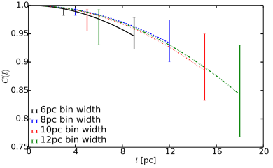
The Taylor microscale, $\lambda$, characterizes the behavior of the correlation function at small scales, $l\to 0$, and can be obtained by fitting the correlation function near the origin to the form

$$C(l)\simeq 1-\left(l/\lambda\right)^{2},$$ (9)

(§6.4 in Tennekes & Lumley, 1972). The associated equality $\mathrm{d}C/\mathrm{d}l=0$ at $l=0$ holds for the correlation functions of smooth (differentiable) random fields (Monin & Yaglom, 1975). In numerical simulations, where the solutions at the smallest scales are controlled by the finite numerical resolution $\Delta x$, one expects $\Delta x<\lambda<l_{0}$ (Davidson, 2004). The Taylor microscale of the random speed can be used to estimate the effective Reynolds number, $\mathrm{Re}$, in the simulations (e.g., §3.2 in Tennekes & Lumley, 1972),

$$\lambda\simeq 3l_{0}\mathrm{Re}^{-1/2}.$$ (10)

Such an estimate includes all dissipation effects in an averaged manner, which can be difficult to estimate otherwise because of the extreme inhomogeneity of the simulated ISM and numerical transport coefficients.

Thus obtained, the Reynolds number is based on the correlation scale of the random flow; the corresponding value based on the domain size ($1\,{\rm kpc}$), often quoted in the literature, is about $400$.

We fit equation (9) to the correlation function $C(l)$ of the random gas speed at the three smallest values of $l$, including $C(l)=1$ at $l=0$, for bin width in $l$ of $6$, $8$, $10$, and $12\,{\rm pc}$. Figure 5 shows the correlation functions obtained at $|z|\leq 50\,{\rm pc}$ and the fits.

The resulting estimates of $\lambda$, shown in Table 2, satisfy the inequalities $\Delta x<\lambda<l_{0}$, providing us some confidence in the estimates of the correlation lengths discussed above. For $l_{0}=60\,{\rm pc}$ (Table 1) and $\lambda=40\,{\rm pc}$, we obtain an estimate of the effective Reynolds number in the simulations of order 20. We also obtained similar results in a model with doubled velocity shear.

The relatively low value of the effective Reynolds number is likely to be a consequence of the shock capturing numerical scheme used in the simulations, where shock fronts are diffused over several grid points to be fully resolved. The maximum Reynolds number achievable with the numerical resolution $\Delta x$ is of order $\mathrm{Re}_{\mathrm{max}}\simeq(l_{0}/\Delta x)^{4/3}$ (assuming a power-law turbulent spectrum with a slope of $5/3$). With $l_{0}=50\,{\rm pc}$, this yields $\mathrm{Re}_{\mathrm{max}}\simeq 30$, so the effective value of $\mathrm{Re}$ measured directly is not much smaller than the nominal value.

We also note that the value of the effective Reynolds number is likely to be much lower than local values in diffuse gas because it includes strong numerical dissipation in shocks.

A comprehensive analysis of vortex generation in the ISM by Käpylä et al. (2017) identifies baroclinicity to be significantly the most efficient source of vorticity in SN driven turbulence. Vorticity is critical to dynamo action, and this conversion of potential into rotational flow may partly explain the persistence of the dynamo even at the relatively low Reynolds numbers, as compared to simulations which model SNe without thermal energy or viscous heating.

The correlation scale of the random flow is controlled by the energy injection mechanism rather than the Reynolds number, so we believe that the modest value of the Reynolds number that our work shares with other comparable simulations does not affect our conclusions.

3.4. Overall statistics and the cold and hot phases

The results presented above are for the warm gas. The data for the cold gas at offsets beyond $l\simeq 10\text{--}100\,{\rm pc}$, the typical scale of the cold gas clouds, are scarce because the cold gas occupies a small fraction of the volume. Furthermore, the numerical resolution of $4\,{\rm pc}$ in our simulations restricts the quality of the modelling of the cold phase, localized in regions of order $10\,{\rm pc}$ in size. Additionally, our results only consider cold gas structures that are typical of diffuse clouds, since we do not model the molecular gas (see Section 2.1).

Figure 6 only shows the cold phase results for the mid-plane, since the cold gas is concentrated there, and results outside this region cannot be statistically meaningful (see Gent, 2012; Gent et al., 2013a). The structure functions for the hot phase fluctuate wildly and have large error bars (see Figure 7). This happens because the hot phase is extremely variable within the relatively small computational box that we have.

A separate analysis for each ISM phase, feasible with simulated data, may not be possible in observations. Therefore, we briefly discuss the statistical properties of the simulated ISM without separation by phase. The results are shown in Table 3.

As shown in Figure 8, the structure and correlation functions of magnetic fluctuations, $b$, for the whole ISM are almost identical to those in the warm phase. This is also true of the gas density fluctuations $n^{\prime}$. This similarity is reflected in the values of $l_{b}$, $l_{n^{\prime}}$, $\sigma_{b}$, and $\sigma_{n^{\prime}}$. This is, of course, largely due to the large fractional volume of the warm phase. It is worth noting, however, that the density and magnetic field strength in the hot phase are both lower than in the warm phase.

However, the values of $\sigma_{u^{\prime}}$ and $l_{u^{\prime}}$ for the whole ISM are significantly higher than in the warm phase. The larger values of $\sigma_{u^{\prime}}$ for the whole ISM can be attributed to the contribution of the hot gas that has higher speed of sound and, correspondingly, higher random velocities.

Figure 9.— Time autocorrelation functions, $C(\tau)$, for the random speed, for $-1000\leq z\leq-550\,{\rm pc}$ (black, solid), $-480\leq z\leq-35\,{\rm pc}$ (blue, dashed), $30\leq z\leq 480\,{\rm pc}$ (red, dash-dotted), and $540\leq z\leq 990\,{\rm pc}$ (green, dash-triple-dotted). The error bars denote the standard deviation of the individual contributions to the correlation function around the mean value. For clarity, only every fourth error bar is shown at each curve.

4. Time correlation

Unlike the correlation lengths of various observable quantities in the ISM, their correlation times cannot be obtained from observations. Because of this, the eddy turnover time $\tau=l_{0}/u_{0}$ is universally applied to interstellar turbulence. However, the dynamics of interstellar turbulence involves a range of physical processes having distinct time scales, which may make the eddy turnover time inappropriate as an estimate of the correlation time. Nonlinear Alfvén wave interactions, shock-wave turbulence and fluctuation dynamo action, among other phenomena, are likely to affect the correlation time and make it different for different variables.

Similarly to correlation lengths, the correlation times can be different in the warm and hot phases. However, this difference is harder to capture since each parcel of warm or hot gas moves around. Therefore, we can only obtain correlation times averaged over the ISM phases.

We consider arguably the most important of the time correlations, that of the random velocity. For this purpose, we use time series of the magnitude of the random velocity measured at an array of fixed points in $32$ planes in $z$, separated by $64\,{\rm pc}$; within each plane, there are $64$ positions separated by $100\,{\rm pc}$ in $x$ or $y$.

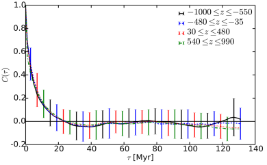
From this data, we can calculate the temporal structure function, and then autocorrelation function $C(\tau)$, from which we obtain the correlation time $\tau_{0}$,

$$\tau_{0}=\int_{0}^{\infty}C(\tau)\;\mathrm{d}\tau\;.$$ (11)

We fit the form in equation (5) to $C(\tau)$ to estimate $\tau_{0}$.

The autocorrelation functions are shown in Figure 9 for four distances from the mid-plane, and the correlation times can be found in Table 4: $\tau_{0}\approx 5\,{\rm Myr}$ with little variation with $|z|$. Since the fractional volumes of the warm and hot gas vary significantly with $|z|$, this suggests that both phases have similar correlation times.

With the velocity correlation length and speed in the warm gas at $z=0$ of $60\,{\rm pc}$ and $8\,{\rm km\,s^{-1}}$, respectively (from Table 1) the kinematic time scale (‘eddy turnover time’) is of order $\tau_{\mathrm{eddy}}=l_{u^{\prime}}/\sigma_{u^{\prime}}\simeq 8\,{\rm Myr}.$ At $|z|=400\,{\rm pc}$, we similarly have $\tau_{\mathrm{eddy}}\simeq 30\,{\rm Myr}$ in the warm gas.

According to the model of interstellar shock-wave turbulence of Bykov & Toptygin (1987), the separation of primary shock fronts driven by supernova explosions depends on their Mach number $M$ as

Table 4 The correlation time of the random speed at various heights in the simulation domain.

$z$	$\tau_{0}$
$[\text{pc}]$	[Myr]
$-1.000\leq z\leq-0.550$	$4.6\pm 0.6$
$-0.480\leq z\leq-0.035$	$4.9\pm 0.5$
$0.030\leq z\leq 0.480$	$4.9\pm 0.7$
$0.540\leq z\leq 0.990$	$4.6\pm 1.0$

$$L_{\text{shock}}\simeq 4M^{4.5}\,{\rm pc}\,,$$ (12)

where the galactic supernova rate of $0.02\,{\rm yr}^{-1}$ has been adopted. The primary shocks dominate over weaker secondary shocks for $M\gtrsim 1.2$, which leads to $L_{\text{shock}}\simeq 10\,{\rm pc}$. The corresponding time between crossings of a given position by shock fronts, which is expected to destroy time correlations, then follows as $\tau_{\rm{shock}}=L_{\rm{shock}}/c\simeq 0.7\,{\rm Myr}$, where $c=14\,{\rm km\,s^{-1}}$ is the magnetosonic speed in the warm gas (assuming equality of the sound and Alfvén speeds).

In the simulations with double rotation rate, the velocity correlation rate and speed at the mid-plane in the warm phase change to $58\,{\rm pc}$ and $8\,{\rm km\,s^{-1}}$, resulting in the eddy turnover time of $\tau_{\rm eddy}\approx 7\,{\rm Myr}$, whereas $\tau_{\rm shock}$ remains unchanged.

Since the estimate of $\tau_{0}$ that we have does not distinguish between the hot and warm phases, it depends on both the kinematic and shock-crossing time scales in each phase (and also the Alfvén time scale, but this is close to the kinematic time scale since the magnetic and kinetic energy densities are comparable). All these time scales are of the same order of magnitude, so more careful estimates of the correlation time are required to clarify the physical nature of the time correlations in the simulated ISM.

It is plausible that the correlation time reflects both time scales and $\tau_{0}^{-1}\simeq\epsilon\tau_{\rm eddy}^{-1}+(1-\epsilon)\tau_{\text{shock}}^{-1}$ with a certain constant $\epsilon$. With $\tau_{0}=5\,{\rm Myr}$, $\tau_{\text{\rm eddy}}=7\,{\rm Myr}$ and $\tau_{\text{shock}}=1\,{\rm Myr}$, we obtain $\epsilon\simeq 0.9$, so the shock waves contribute about 10% to the random flow in this sense.

Figure 10.— Autocorrelation functions, $C(l)$ for magnetic field components, averaged at heights; a) $z=-400\,{\rm pc}$, b) $z=0\,{\rm pc}$ and c) $z=400\,{\rm pc}$.

The time autocorrelation function of Fig. 9 appears to vary around the zero level at a time scale of about $70\,{\rm Myr}$. Although the accuracy of the autocorrelation values is higher than suggested by the scatter of the data points around the mean values shown by the error bars, the statistical significance of these variations is unclear. Physical interpretation of the time correlation function is also hampered by the fact that we do not have time series for the variables in the warm and hot phases separately.

We note, however, that the apparent time scale of the variations is close to the period $(2\pi\lambda/g_{z})^{1/2}$ of gravity waves of wavelength $\lambda=1\,{\rm kpc}$ in the Galactic gravity field, $g_{z}\simeq 4\times 10^{-9}\,{\rm cm}\,{\rm s}^{-2}$. Oscillatory large-scale horizontal vortical flows have been found by Käpylä et al. (2017) in similar simulations without a magnetic field. For the parameters relevant to the current study, the period of these oscillations is about $50\,{\rm Myr}$. Extending this analysis over a range of rotation rates, SN rates and forms of the gravitational potential may clarify the significance of the pattern in the temporal correlation function apparent in Fig. 9.

Table 5The rms values for each component of the random magnetic field, denoted $b_{0i}$ for $i\in(x,y,z)$, and their correlation lengths.

	$b_{0i}$ [nG]			$l_{0}\,[\rm pc]$			$\tilde{l}_{0}\,[\rm pc]$
$|z|$ [pc]	$0$	$400$		$0$	$400$		$0$	$400$
$b_{x}$	$549\pm 1$	$432\pm 1$		$46\pm 2$	$51\pm 3$		$33\pm 1$	$32\pm 1$
$b_{y}$	$676\pm 1$	$524\pm 1$		$41\pm 1$	$47\pm 3$		$36\pm 1$	$36\pm 1$
$b_{z}$	$692\pm 1$	$667\pm 2$		$59\pm 3$	$65\pm 3$		$16\pm 1$	$14\pm 1$

5. Anisotropy of the magnetic field

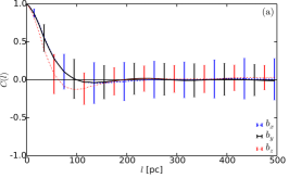
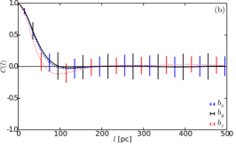
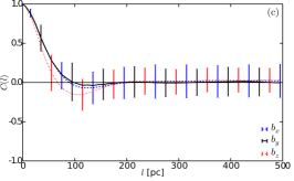
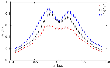
In the analysis above, we neglected any anisotropy of the random magnetic field in the horizontal planes. This is justifiable since, at the scales of interest (from a few parsecs to about $100\,{\rm pc}$), the expected anisotropy is only moderate (see below). However, the anisotropy of magnetic fields is of high physical significance as it reflects the dynamics of MHD turbulence with and without a global mean magnetic field (Goldreich & Sridhar (1997); Brandenburg & Lazarian (2013) and references therein; see also Cho & Vishniac (2000); Cho & Lazarian (2002a, 2003b); Mallet et al. (2016) and Oughton et al. (2016)). It also reflects the effects of galactic differential rotation and compression of the random magnetic field in shocks. The anisotropy of interstellar magnetic fields can contribute significantly to the polarized radio emission of galaxies (e.g., Sokoloff et al., 1998; Beck, 2016). In this section, using the structure and autocorrelation functions, we discuss individual components of the random magnetic field, $\bm{b}=(b_{x},b_{y},b_{z})$ denoting their rms values $b_{0x}$, $b_{0y}$ and $b_{0z}$.

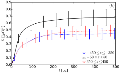
As shown in Table 5, the three components of $\bm{b}$ are somewhat different in magnitude. The vertical, $z$-components is the largest at all heights, whereas the radial ($x$) random field is the weakest.

All three components of magnetic field have negative autocorrelation near $l=100\,{\rm pc}$, stronger for $b_{z}$ than for $b_{x}$ and $b_{y}$. This appears to be a consequence of the solenoidality of magnetic field: since magnetic lines must be closed, magnetic field must, on average, change its direction at a length scale comparable to its correlation length.

An enhanced azimuthal ($y$) component is a result of the large-scale velocity shear due to differential rotation that produces $b_{y}$ from the radial field $b_{x}$, so that $\partial b_{y}/\partial t\simeq q\Omega b_{x}$ and then (e.g., Stepanov et al., 2014)

$$b_{0y}\simeq(1+q\Omega\tau_{0})b_{0x}.$$ (13)

For $q=+1$, $\Omega=25\,{\rm km\,s^{-1}}\,{\rm kpc}^{-1}$ and $\tau_{0}=5\,{\rm Myr}$, this yields $b_{0y}/b_{0x}\simeq 1.2\text{--}1.3$, in agreement with the estimates of Table 5 at $z=0$.

Figure 11.— The rms values of the components of the random magnetic field vector as functions of distance to the mid-plane: the radial $b_{0x}$ (red, triangles), azimuthal $b_{0y}$ (black, circles), and vertical $b_{0z}$ (blue, squares) random magnetic fields.

The vertical component of the magnetic field is similarly enhanced beyond isotropy due to the stretching of the horizontal magnetic field by vertical velocity $u_{z}$ that varies at a scale $l_{0}$ and yet has a mean part $\overline{u}_{z}\simeq 2\,{\rm km\,s^{-1}}$ at $|z|\lesssim 200\,{\rm pc}$: $\partial b_{z}/\partial t\simeq b_{x}\partial u_{z}/\partial x+b_{y}\partial u_{z}/\partial y$. Unlike the stretching of the radial magnetic field by the large-scale velocity shear, this is a random process, so the rms vertical magnetic field grows as $t^{1/2}$. With the radial field $b_{x}$ representing the isotropic background, this leads to the estimate

$$\frac{b_{0z}}{b_{0x}}\simeq\left[1+\frac{\tau_{0}\overline{u}_{z}}{l_{0}}\left(1+\frac{b_{0x}^{2}}{b_{0y}^{2}}\right)\right]^{1/2}\simeq 1.2\,,$$

in a reasonable agreement with the estimates of Table 5. Since the vertical component of the random magnetic field is produced from both of its horizontal components, the $z$-component is the strongest one.

An important radio astronomical consequence of the magnetic anisotropy is polarization of the synchrotron emission. If our simulation domain was observed from the top or bottom (i.e., along the $z$ direction) the observed degree of polarization due to the random magnetic field alone would be (Laing, 1981; Sokoloff et al., 1998, 1999)

$$p=p_{0}\frac{|b_{0x}^{2}-b_{0y}^{2}|}{b_{0x}^{2}+b_{0y}^{2}}\approx 0.15,$$

where $p_{0}\approx 0.7$ is the maximum intrinsic degree of polarization, and we have neglected, for the sake of the argument, both depolarization effects and the average magnetic field. Such a degree of polarization is comparable to that observed in spiral galaxies, suggesting that the anisotropy of the interstellar random magnetic fields needs to be allowed for in the interpretations of radio polarization observations of spiral galaxies (cf. Beck, 2016).

The correlation lengths of the magnetic field components are given in Table 5 (for comparison with Table 1). Because of the stretching of radial magnetic field by differential rotation that produces a stronger azimuthal field, we might expect the azimuthal correlation length to be larger than the radial one (Moffatt, 1967; Terry, 2000), contrary to the results in Table 5, where the correlation lengths for $b_{x}$ and $b_{y}$ are of similar magnitude. However, the correlation lengths were calculated using isotropic horizontal position lags, whereas azimuthal ($y$) and radial ($x$) lags should be considered separately to detect the expected difference in the correlation lengths in the two directions. Such a refined calculation requires a larger data domain to provide sufficient statistics. Houde et al. (2013) find that $l_{0y}\approx 1.8l_{0x}$ for the random magnetic field, i.e., the magnetic correlation length approximately along the mean-field direction ($y$ in our case) is about twice that in the perpendicular direction, and this ratio is similar to the ratio of $b_{0y}/b_{0x}$ found by these authors from depolarization of the synchrotron emission. The vertical magnetic field component has significant anticorrelation at $l\approx 100\,{\rm pc}$, shown in Figure 10, which results in very different values of $l_{0}$ and $\tilde{l}_{0}$, similar to $n^{\prime}$.

As shown in Figure 11, individual components of the random magnetic field vary differently with $|z|$. As with the mean magnetic field, the rms means first increase with distance from the mid-plane until $|z|\approx 200\,{\rm pc}$, and only then decrease. As suggested above, both $b_{y}$ and $b_{z}$ are enhanced, in comparison with $b_{x}$, by the horizontal velocity shear and random vertical flows, respectively; correspondingly, $b_{0y}$ and $b_{0z}$ increase with $|z|$ faster than $b_{0x}$ at $|z|\lesssim 200\,{\rm pc}$, but then decrease with $|z|$ following the decrease in $b_{0x}$. At $|z|\geq 300\,{\rm pc}$, each component of $\bm{b}$ decreases nearly exponentially with the scale height of about $450\,{\rm pc}$.

Simulations with double rotation rate produce similar results.

6. Observable quantities

The main observational tools employed in the analysis of interstellar MHD turbulence are Faraday rotation and synchrotron emission, both total and polarized. Their statistical properties and their relation to the underlying random distributions of magnetic fields, gas density and cosmic rays have received significant attention, both observationally and theoretically (see references in §1). Here we discuss correlation properties of the observable quantities in the simulated ISM. Given that magnetic field and gas density can have different correlation functions, and can be correlated with each other (Beck et al., 2003), statistical properties of the observable quantities are difficult to predict with confidence.

Both Faraday rotation and synchrotron emission depend on the relative orientation of the large-scale magnetic field and the line of sight. The mean magnetic field in the simulations used here is predominantly horizontal and its $y$-component is the strongest (Gent et al., 2013a, b). Exploring the observational appearance of the simulated volume from various vantage points will be our goal elsewhere; here we only discuss the properties of fluctuations in Faraday rotation and synchrotron emission using just one direction of ‘observation’.

Figure 12.— The autocorrelation function of the Faraday depth $\phi(x,y)$. The error bars represent the scatter of the data points around the mean values shown with solid line.

Table 6 The rms values and the correlation lengths for electron density $n_{e}$.

$|z|$		rms		$l_{0}$
[pc]		[$\rm cm^{-3}$]		$[\rm pc]$
$0$		$0.2560\pm 0.0007$		$59\pm 3$
$200$		$0.1665\pm 0.0008$		$61\pm 5$
$400$		$0.0530\pm 0.0003$		$80\pm 6$
$600$		$0.0208\pm 0.0002$		$93\pm 8$
$800$		$0.0083\pm 0.0001$		$83\pm 7$

Figure 13.— Structure functions of the synchrotron intensity assuming (a) constant cosmic ray density, $I$; and (b) local energy equipartition, $I_{\mathrm{eq}}$. Vertical dashed lines represent the standard deviation of the individual data points around the mean value shown with solid line, whereas error bars show the accuracy of the mean. The computational volume is ‘observed’ at roughly the right angle to the mean magnetic field, similarly to Milky Way observations at high Galactic latitudes.

6.1. Faraday depth

The Faraday depth of a magneto-ionic region is an integral along the line of sight, assumed here to be along the $z$-direction for convenience:

$$\phi(x,y)=0.81\int_{-L_{z}}^{L_{z}}n_{\text{e}}B_{z}\,\mathrm{d}z\;\,{\rm rad\,m^{-2}},$$ (14)

where $n_{\mathrm{e}}$ is the number density of thermal electrons in cm^-3, $B_{z}$ is the line-of-sight component of magnetic field in $\mu$G, distance $z$ is in $\rm pc$, and $L_{z}$ is the half-size of the computational domain along $z$. Since the mean magnetic field is nearly horizontal, the mean value of $B_{z}$ is close to zero together with the mean Faraday depth along this direction.

Our simulations do not include gas ionization and only provide total gas density $n$. Since interstellar plasmas can be far from ionization equilibrium (de Avillez & Breitschwerdt, 2012a, b), we obtain thermal electron density from a heuristic relation that ensures that the mean electron number density is about $0.03\,{\rm cm}^{-3}$ and the gas is fully ionized at $T\gtrsim 10^{5}\,{\rm K}$:

$$n_{\mathrm{e}}=n\left[\frac{\mathrm{arctan}(T/10^{3}\,{\rm K}-10)}{\pi}+\frac{1}{2}\right].$$ (15)

Since observations do not distinguish between different ISM phases, the Faraday depth has been computed for the whole computational domain.

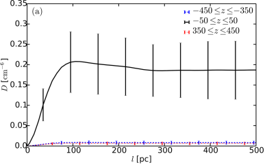
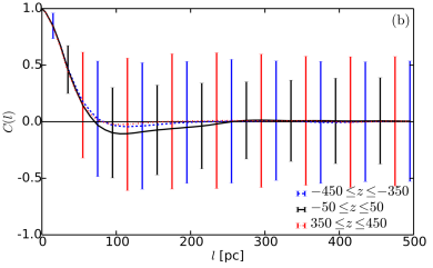
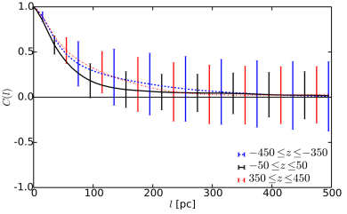
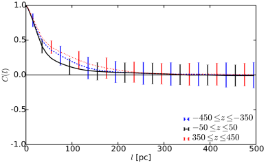
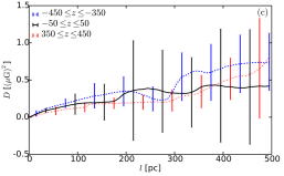
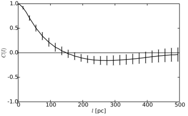
The autocorrelation function of the Faraday depth is shown in Figure 12. Its correlation length, $l_{\phi}=122\pm 12\,{\rm pc}$ is significantly greater than the correlation length of electron density, $60\,{\rm pc}$ at the midplane increasing to $80\,{\rm pc}$ at $|z|=800\,{\rm pc}$ (Table 6), and the vertical random magnetic field, $60\,{\rm pc}$ (Table 5). We note that the mean component of $B_{z}$ is negligible, so that the mean value of the Faraday depth is close to zero, $\langle\phi\rangle=2.88\pm 6.42\,\text{rad\,m}^{-2}$.

As discussed by Beck et al. (2003), the magnitude of Faraday rotation depends on the correlation between magnetic field and thermal electron density. To clarify their relation in our simulations, we computed the cross-correlation coefficient between $n_{\text{e}}$ and $B_{z}$ separately for the warm and hot gas:

$$r=\frac{\overline{(n_{\text{e}}-\overline{n}_{\text{e}})\left(B_{z}-\overline{B}_{z}\right)}}{\overline{(n_{\text{e}}-\overline{n_{\text{e}}})^{2}}^{1/2}\,\overline{(B_{z}-\overline{B}_{z})^{2}}^{1/2}}\,$$ (16)

where the overbar denotes an average taken over the volume occupied by the phase. The results, averaged over the snapshots, confidently suggest that the two variables are uncorrelated: $r=0.02\pm 0.02$ in the warm gas and $0.07\pm 0.04$ in the hot phase.

The autocorrelation of $\phi$ is negative at $l\gtrsim 150\,{\rm pc}$. Both magnetic field (Section 5) and gas density have negative autocorrelation at these scales (Fig. 2). Quantitative assessment of this feature should await a more detailed analysis of the ionization structure of the modelled ISM, but we note that this behaviour can have important implications for the interpretation of radio polarization observations of the ISM, in terms of parameters of interstellar turbulence.

Figure 14.— As in Figure 13 but for polarized intensity assuming (a) constant cosmic ray density, $P$, and (b) local energy equipartition, $P_{\rm eq}$.

6.2. Synchrotron intensity

Statistical properties of the synchrotron intensity are sensitive to the relation between the distributions of cosmic ray electrons, $n_{\text{cr}}$, and magnetic field. Cosmic rays (Berezinskiĭ et al., 1990) have a high diffusivity of order $3\times 10^{28}\,{\rm cm}^{2}\,{\rm s}^{-1}$, so their diffusion length over the confinement time of $10^{6}\,{\rm yr}$ is of order $1\,{\rm kpc}$. Thus, it can be expected that cosmic rays are distributed much more homogeneously than magnetic fields, but the assumption of a local energy equipartition (or pressure balance) between cosmic rays and magnetic fields is often used in interpretations of synchrotron observations (e.g., Beck & Krause, 2005). We note that analysis of synchrotron fluctuations in spiral galaxies suggest that cosmic ray electrons and magnetic fields can be slightly anti-correlated (Stepanov et al., 2014). Fluctuations of synchrotron intensity can provide information about interstellar turbulence (Lazarian & Pogosyan, 2012, 2016). Here we discuss the synchrotron intensity fluctuations implied by our ISM simulations.

The synchrotron intensity, in arbitrary units, is obtained by integration along the $z$-axis (so that the mean magnetic field is mostly perpendicular to the line of sight),

$$I(x,y)=\int_{-L_{z}}^{L_{z}}n_{\text{cr}}\left(B_{x}^{2}+B_{y}^{2}\right)\,\mathrm{d}z,$$ (17)

using two alternative assumptions about cosmic ray distribution $n_{\text{cr}}$:

$$n_{\text{cr}}=\text{const}\,,$$

and

$$n_{\text{cr}}\propto B^{2}\,.$$

As with the Faraday depth, we do not consider other lines of sight through the computational domain.

The Stokes parameters, at wavelengths short enough that Faraday rotation is negligible, are similarly obtained as

$$Q(x,y) =\int_{-L_{z}}^{L_{z}}\cos(2\psi_{0})n_{\text{cr}}(B_{x}^{2}+B_{y}^{2})\,\mathrm{d}z,$$ (18)

$$U(x,y) =\int_{-L_{z}}^{L_{z}}\sin(2\psi_{0})n_{\text{cr}}(B_{x}^{2}+B_{y}^{2})\,\mathrm{d}z,$$ (19)

where $\psi_{0}(\bm{x})$ is the intrinsic polarization angle perpendicular to the local magnetic field in the $(xy)$-plane, calculated as $\psi_{0}=\pi/2+\arctan(B_{y}/B_{x})$. The polarized intensity follows as

$$P(x,y)=\sqrt{Q^{2}+U^{2}}.$$ (20)

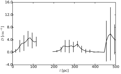
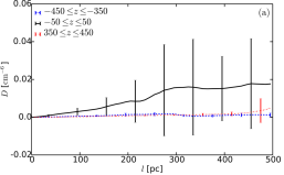
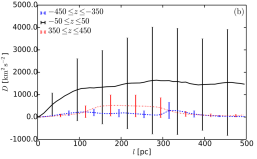
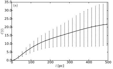
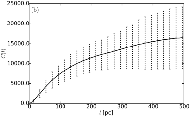
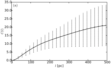
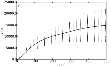
The structure functions of the total and polarized synchrotron intensities under both assumptions about the cosmic ray distribution are shown in Figures 13 and 14, respectively. They clearly have a more complicated form than those of the magnitude of the random magnetic field shown in Figure 4. This is not surprising since the mean field is a function of position, and hence contributes to the structure and correlation functions. In particular, the systematic increase of the structure function at large values of $l$ results from this contribution. The contribution from the mean field needs to be subtracted from the structure function before any further analysis could be done. We postpone such analysis to simulations that include cosmic rays.

A notable feature of the results illustrated in Figures 13 and 14 is the rapid increase in the scatter of the data points and the deterioration of the accuracy of the structure function estimates as the lag $l$ becomes larger than about $200\,{\rm pc}$. This is understandable since the synchrotron emissivity depends on relatively high power of the fluctuating magnetic field. Observations in the Milky Way can be especially strongly affected, because even within a narrow telescope beam the divergence of the lines of sight can be as wide as hundreds of parsecs at some distance from the Sun (Cho & Lazarian, 2002b, 2003a, 2010).

In the case of external galaxies, a linear resolution of order a few hundred parsecs is typical of synchrotron observations. The increase in the uncertainty of the correlation function with $l$ can cause serious complications in the analysis of interstellar turbulence using power spectra of synchrotron fluctuations (the Fourier transforms of the correlation function) as suggested by Lazarian & Pogosyan (2012, 2016) and Lee et al. (2016). This problem may not be evident when power spectra are considered because it is difficult to estimate their statistical accuracy. However, correlation analysis, with due attention to the errors, makes the problem evident.

7. Discussion

We have performed detailed correlation analysis of the random physical fields in extensive ISM simulations, focusing mainly on the warm gas since it occupies a larger part of the volume. Statistical properties of the fluctuations in the gas properties are strongly non-Gaussian because of widespread filamentary and planar, small-scale structures. Such features cannot be captured by second-order correlation functions (or their equivalent, power spectra) and require other tools sensitive to all statistical moments of the random field, such as Minkowski functionals (e.g., Wilkin et al., 2007; Makarenko et al., 2015, and references therein) and topological data analysis (Adler et al., 2010; Edelsbrunner, 2014). However, careful correlation analysis remains a necessary first step in the exploration of statistical properties of random fields.

There are two difficulties in correlation analysis (and its equivalent, power spectrum analysis) that deserve special attention as they also occur in any exploration of either simulated or observational data. Correlation analysis is only meaningful when applied to a random distribution. Therefore, random fluctuations in physical parameters need to be isolated first by subtracting their averaged distributions. Averaging is straightforward in infinite domains with statistically homogeneous fluctuations. However, in reality the domain can contain only a modest number of correlation volumes, and the mean distributions of physical variables are not necessarily uniform or describable via a simple trend. We obtain the averaged distributions using Gaussian smoothing at a scale (half-width of the Gaussian window) of $50\,{\rm pc}$ chosen carefully as in Gent et al. (2013b) (see Section 2.3). Simpler procedures, for example using a uniform mean value at a given $z$, distort the results because of the contamination of the structure and correlation functions by systematic and complicated non-random trends. In particular, the values of correlations lengths obtained under the assumption of horizontally uniform mean values are unphysically large, exceeding $200\,{\rm pc}$.

Even with a correlation lengths $l_{0}$ of less than $100\,{\rm pc}$, the finite size of the domain (of order $1\,{\rm kpc}^{3}$ in our case) can significantly affect the estimated values of $l_{0}$, as the integration in Equation (4) extends to infinity. We resolve this problem by fitting the measured correlation functions with physically motivated forms, which can then be integrated over an infinite range. The difference between the correlations lengths obtained with and without this fitting can be as large as a factor of two.

Given the complex structure of the simulated ISM, it is not surprising that different physical variables have different correlation functions and different correlation lengths $l_{0}$, as shown in Table 1. The observational estimates available for the correlations lengths in the ISM provide a wide range of values depending on the quantity observed. Conclusive comparison with observations requires detailed knowledge of the statistical properties of the random fields involved and their cross-correlations (Stepanov et al., 2014). Interstellar turbulence cannot be characterized by a single correlation length.

We have estimated the correlation time of the velocity fluctuations $\tau_{0}$. In the simulations used here,$\tau_{0}\simeq 5\,{\rm Myr}$ is close to both the eddy turnover time, $\tau_{\mathrm{eddy}}\simeq 8\,{\rm Myr}$ and the estimated time interval between the passage of shock fronts through a given position, $\tau_{\mathrm{shock}}\simeq 1\,{\rm Myr}$. The correlation time is likely to be sensitive to the supernova rate (and then, star formation rate) and may be closer to $\tau_{\mathrm{shock}}$ when the supernova rate is higher. Further calculations with varying supernova rates are needed to explore under what conditions either physical process dominates the correlation time.

The random magnetic field is noticeably anisotropic, with larger rms values for azimuthal ($y$) and vertical ($z$) components in comparison to the radial ($x$) component, with $b_{z}$ the strongest component. The enhanced $y$-component is produced by the action of the large-scale velocity shear on the radial turbulent magnetic field $b_{x}$, with the enhanced $z$ component produced by stretching of the horizontal magnetic field by the random part of the vertical velocity $u_{z}$. From the rms values of $b_{x}$ and $b_{y}$, we estimate a degree of polarization of $p\approx 0.15$ that may be produced by the magnetic anisotropy.

We also performed correlation analysis of the Faraday depth along the vertical direction through the computational domain. Its correlation scale, $120\,{\rm pc}$, is significantly larger than the correlation scales of electron density ($60\text{--}90\,{\rm pc}$) and of vertical magnetic field ($60\,{\rm pc}$). This suggests that there is no simple and universal relationship between the correlation scales of electron density, vertical magnetic field and Faraday depth.

Analysis of the total and polarized synchrotron intensities is hampered by a rapid increase of the scatter of data points around the average contributions to the structure and correlation functions. This difficulty is evident in the correlation analysis but would not be apparent in the power spectra, where statistical errors are difficult to estimate.

Appendix A Comparison with larger domain

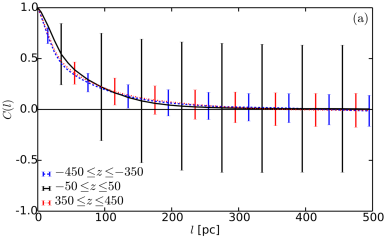
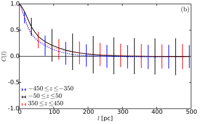
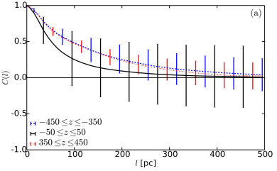
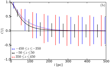
The computational domain used to obtain our results, about $1\times 1\times 2\,{\rm kpc}^{3}$, contains only about $10^{3}$ correlation cells and, in addition, may be too small to accommodate the most rapidly growing mode of the large-scale magnetic field. The large-scale dynamo remains in its kinematic stage in the larger domain, but otherwise the simulation has achieved a statistically steady state. Therefore, we verify the results using similar simulations in a larger domain, approximately $1.532\times 1.532\times 2.556\,\,{\rm kpc}^{3}$ in size. The velocity shear rate is that of the Solar neighborhood, $q=-1$, and we analyze data from $12$ snapshots in the range $0.336\leq t\leq 0.6\,{\rm Gyr}$, with a separation of $24\,{\rm Myr}$. The extended domain is not designed to capture fountain flows (see Section 2.1) but is instead employed to to test how robust our results are to the horizontal area of the simulation.

The results from the larger domain are compared with those obtained from the kinematic stage of the large-scale dynamo in the main run discussed in the text. We use data from 21 snapshots in the range $0.4\leq t\leq 0.61\,\mathrm{Gyr}$, with a separation of $10\,\mathrm{Myr}$.

We find very similar correlations in $b$ between the two runs (see Figure 15 and Table 7), but there are more significant differences for $u^{\prime}$ (see Figure 16 and Table 7; the latter also gives comparable statistics for a similar kinematic state in the standard domain). The correlation lengths of $u^{\prime}$ are actually smaller for the larger domain, so the difference does not simply result from velocity structures having been restricted in size. In light of the differences noted above, further simulations are needed before a direct comparison can be made.

References

- Adler et al. (2010) Adler, R. J., Bobrowski, O., Borman, M. S., Subag, E., & Weinberger, S. 2010, in IMS Collections, Vol. 6, Borrowing Strength: Theory Powering Applications, 124–143
- Beck (2016) Beck, R. 2016, A&A Rev., 24, 4, 1509.04522
- Beck et al. (2005) Beck, R., Fletcher, A., Shukurov, A., Snodin, A., Sokoloff, D. D., Ehle, M., Moss, D., & Shoutenkov, V. 2005, A&A, 444, 739, astro-ph/0508485
- Beck & Krause (2005) Beck, R., & Krause, M. 2005, Astronomische Nachrichten, 326, 414, astro-ph/0507367
- Beck et al. (2003) Beck, R., Shukurov, A., Sokoloff, D., & Wielebinski, R. 2003, A&A, 411, 99, astro-ph/0307330
- Bendre et al. (2015) Bendre, A., Gressel, O., & Elstner, D. 2015, Astronomische Nachrichten, 336, 991, 1510.04178
- Berezinskiĭ et al. (1990) Berezinskiĭ, V. S., Bulanov, S. V., Dogiel, V. A., Ginzburg, V. L. e., & Ptuskin, V. S. 1990, Astrophysics of Cosmic Rays. (Amsterdam: North Holland)
- Brandenburg & Lazarian (2013) Brandenburg, A., & Lazarian, A. 2013, Space Sci. Rev., 178, 163, 1307.5496
- Brown & Taylor (2001) Brown, J. C., & Taylor, A. R. 2001, ApJ, 563, L31
- Bykov & Toptygin (1987) Bykov, A. M., & Toptygin, I. N. 1987, Ap&SS, 138, 341
- Cho & Lazarian (2002a) Cho, J., & Lazarian, A. 2002a, Physical Review Letters, 88, 245001, astro-ph/0205282
- Cho & Lazarian (2002b) ——. 2002b, ApJ, 575, L63, astro-ph/0205284
- Cho & Lazarian (2003a) ——. 2003a, New A Rev., 47, 1143, astro-ph/0306183
- Cho & Lazarian (2003b) ——. 2003b, MNRAS, 345, 325, astro-ph/0301062
- Cho & Lazarian (2010) ——. 2010, ApJ, 720, 1181, 1007.3740
- Cho & Vishniac (2000) Cho, J., & Vishniac, E. T. 2000, ApJ, 539, 273, astro-ph/0003403
- Davidson (2004) Davidson, P. A. 2004, Turbulence : an introduction for scientists and engineers (OUP Oxford)
- de Avillez & Breitschwerdt (2005) de Avillez, M. A., & Breitschwerdt, D. 2005, A&A, 436, 585, astro-ph/0502327
- de Avillez & Breitschwerdt (2007) ——. 2007, ApJ, 665, L35, 0707.1740
- de Avillez & Breitschwerdt (2012a) ——. 2012a, ApJ, 761, L19
- de Avillez & Breitschwerdt (2012b) ——. 2012b, ApJ, 756, L3
- Edelsbrunner (2014) Edelsbrunner, H. 2014, A Short Course in Computational Geometry and Topology (Berlin: Springer)
- Elmegreen & Scalo (2004) Elmegreen, B. G., & Scalo, J. 2004, ARA&A, 42, 211, astro-ph/0404451
- Federrath et al. (2010) Federrath, C., Roman-Duval, J., Klessen, R. S., Schmidt, W., & Mac Low, M.-M. 2010, A&A, 512, A81, 0905.1060
- Fletcher et al. (2011) Fletcher, A., Beck, R., Shukurov, A., Berkhuijsen, E. M., & Horellou, C. 2011, MNRAS, 412, 2396, 1001.5230
- Gaensler et al. (2005) Gaensler, B. M., Haverkorn, M., Staveley-Smith, L., Dickey, J. M., McClure-Griffiths, N. M., Dickel, J. R., & Wolleben, M. 2005, Science, 307, 1610
- Gent (2012) Gent, F. A. 2012, PhD thesis, Newcastle University School of Mathematics and Statistics, http://ethos.bl.uk/OrderDetails.do?uin=uk.bl.ethos.576746
- Gent et al. (2013a) Gent, F. A., Shukurov, A., Fletcher, A., Sarson, G. R., & Mantere, M. J. 2013a, MNRAS, 432, 1396, 1204.3567
- Gent et al. (2013b) Gent, F. A., Shukurov, A., Sarson, G. R., Fletcher, A., & Mantere, M. J. 2013b, MNRAS, 430, L40, 1206.6784
- Germano (1992) Germano, M. 1992, Journal of Fluid Mechanics, 238, 325
- Goldreich & Sridhar (1997) Goldreich, P., & Sridhar, S. 1997, ApJ, 485, 680, astro-ph/9612243
- Haverkorn et al. (2008) Haverkorn, M., Brown, J., Gaensler, B., & McClure, N. 2008, ApJ, 680, 362
- Haverkorn et al. (2006) Haverkorn, M., Gaensler, B. M., Brown, J. C., Bizunok, N. S., McClure-Griffiths, N. M., Dickey, J. M., & Green, A. J. 2006, ApJ, 637, L33
- Haverkorn et al. (2004) Haverkorn, M., Gaensler, B. M., McClure-Griffiths, N. M., Dickey, J. M., & Green, A. J. 2004, ApJ, 609, 776
- Haverkorn & Spangler (2013) Haverkorn, M., & Spangler, S. R. 2013, Space Sci. Rev., 178, 483, 1304.1735
- Hawley et al. (1995) Hawley, J. F., Gammie, C. F., & Balbus, S. A. 1995, ApJ, 440, 742
- Heiles & Troland (2003) Heiles, C., & Troland, T. H. 2003, ApJ, 586, 1067, astro-ph/0207105
- Hill et al. (2012) Hill, A. S., Joung, M. R., Mac Low, M. M., Benjamin, R. A., Haffner, L. M., Klingenberg, C., & Waagan, K. 2012, ApJ, 750, 104, 1202.0552
- Houde et al. (2013) Houde, M., Fletcher, A., Beck, R., Hildebrand, R. H., Vaillancourt, J. E., & Stil, J. M. 2013, ApJ, 766, 49
- Iacobelli et al. (2013) Iacobelli, M. et al. 2013, A&A, 558, A72, 1308.2804
- Jaffe et al. (2011) Jaffe, T. R., Banday, A. J., Leahy, J. P., Leach, S., & Strong, A. W. 2011, MNRAS, 416, 1152
- Jaffe et al. (2013) Jaffe, T. R. et al. 2013, MNRAS, 431, 683
- Jaffe et al. (2010) Jaffe, T. R., Leahy, J. P., Banday, A. J., Leach, S. M., Lowe, S. R., & Wilkinson, A. 2010, MNRAS, 401, 1013
- Jansson & Farrar (2012a) Jansson, R., & Farrar, G. R. 2012a, ApJ, 761, L11
- Jansson & Farrar (2012b) ——. 2012b, ApJ, 757, 14
- Joung & Mac Low (2006) Joung, M. K. R., & Mac Low, M.-M. 2006, ApJ, 653, 1266, astro-ph/0601005
- Kaplan (1966) Kaplan, S. A. 1966, Interstellar Gas Dynamics (Oxford: Pergamon)
- Käpylä et al. (2017) Käpylä, M. J., Gent, F. A., Väisälä, M. S., & Sarson, G. R. 2017, ArXiv e-prints, 1705.08642
- Korpi et al. (1999a) Korpi, M. J., Brandenburg, A., Shukurov, A., & Tuominen, I. 1999a, A&A, 350, 230
- Korpi et al. (1999b) Korpi, M. J., Brandenburg, A., Shukurov, A., Tuominen, I., & Nordlund, Å. 1999b, ApJ, 514, L99
- Laing (1981) Laing, R. A. 1981, ApJ, 248, 87
- Lazarian & Pogosyan (2012) Lazarian, A., & Pogosyan, D. 2012, ApJ, 747, 5, 1105.4617
- Lazarian & Pogosyan (2016) ——. 2016, ApJ, 818, 178, 1511.01537
- Lazaryan & Shutenkov (1990) Lazaryan, A. L., & Shutenkov, V. P. 1990, Soviet Astronomy Letters, 16, 297
- Lee et al. (2016) Lee, H., Lazarian, A., & Cho, J. 2016, ApJ, 831, 77
- Mac Low et al. (2005) Mac Low, M.-M., Balsara, D. S., Kim, J., & de Avillez, M. A. 2005, ApJ, 626, 864, astro-ph/0410734
- Mac Low & Klessen (2004) Mac Low, M.-M., & Klessen, R. S. 2004, Rev. Mod. Phys., 76, 125, astro-ph/0301093
- Makarenko et al. (2015) Makarenko, I., Fletcher, A., & Shukurov, A. 2015, MNRAS, 447, L55, 1407.4048
- Mallet et al. (2016) Mallet, A., Schekochihin, A. A., Chandran, B. D. G., Chen, C. H. K., Horbury, T. S., Wicks, R. T., & Greenan, C. C. 2016, MNRAS, 459, 2130, 1512.01461
- Minter & Spangler (1996) Minter, A. H., & Spangler, S. R. 1996, ApJ, 458, 194
- Moffatt (1967) Moffatt, H. K. 1967, in Atmospheric Turbulence and Radio Wave Propagation, ed. A. M. Yanglom & V. I. Tatarsky (Moscow: Nauka), 139–154
- Monin & Yaglom (1975) Monin, A. S., & Yaglom, A. M. 1975, Statistical fluid mechanics: Mechanics of turbulence (Cambridge, Mass.: MIT Press)
- Ohno & Shibata (1993) Ohno, H., & Shibata, S. 1993, MNRAS, 262, 953
- Oughton et al. (2016) Oughton, S., Matthaeus, W. H., Wan, M., & Parashar, T. 2016, Journal of Geophysical Research (Space Physics), 121, 5041
- Sánchez-Salcedo et al. (2002) Sánchez-Salcedo, F. J., Vázquez-Semadeni, E., & Gazol, A. 2002, ApJ, 577, 768, astro-ph/0203067
- Sarazin & White (1987) Sarazin, C. L., & White, III, R. E. 1987, ApJ, 320, 32
- Scalo & Elmegreen (2004) Scalo, J., & Elmegreen, B. G. 2004, ARA&A, 42, 275, astro-ph/0404452
- Shneider et al. (2014) Shneider, C., Haverkorn, M., Fletcher, A., & Shukurov, A. 2014, A&A, 568, A83
- Shukurov et al. (2004) Shukurov, A., Sarson, G. R., Nordlund, Å., Gudiksen, B., & Brandenburg, A. 2004, Ap&SS, 289, 319, astro-ph/0212260
- Sokoloff et al. (1998) Sokoloff, D. D., Bykov, A. A., Shukurov, A., Berkhuijsen, E. M., Beck, R., & Poezd, A. D. 1998, MNRAS, 299, 189
- Sokoloff et al. (1999) ——. 1999, MNRAS, 303, 207
- Stepanov et al. (2014) Stepanov, R., Shukurov, A., Fletcher, A., Beck, R., La Porta, L., & Tabatabaei, F. 2014, MNRAS, 437, 2201, 1205.0578
- Tennekes & Lumley (1972) Tennekes, H., & Lumley, J. L. 1972, First Course in Turbulence (MIT Press)
- Terry (2000) Terry, P. W. 2000, Reviews of Modern Physics, 72, 109
- Vázquez-Semadeni (2015) Vázquez-Semadeni, E. 2015, in Astrophysics and Space Science Library, Vol. 407, Magnetic Fields in Diffuse Media, ed. A. Lazarian, E. M. de Gouveia Dal Pino, & C. Melioli, 401
- Wang et al. (2016) Wang, K., Testi, L., Burkert, A., Walmsley, C. M., Beuther, H., & Henning, T. 2016, ApJS, 226, 9, 1607.06452
- Wilkin et al. (2007) Wilkin, S. L., Barenghi, C. F., & Shukurov, A. 2007, Physical Review Letters, 99, 134501, astro-ph/0702261
- Wolfire et al. (1995) Wolfire, M. G., Hollenbach, D., McKee, C. F., Tielens, A. G. G. M., & Bakes, E. L. O. 1995, ApJ, 443, 152