A simulation technique for slurries interacting with moving parts and deformable solids with applications

Abstract

A numerical method for particle-laden fluids interacting with a deformable solid domain and mobile rigid parts is proposed and implemented in a full engineering system. The fluid domain is modeled with a lattice Boltzmann representation, the particles and rigid parts are modeled with a discrete element representation, and the deformable solid domain is modeled using a Lagrangian mesh. The main issue of this work, since separately each of these methods is a mature tool, is to develop coupling and model-reduction approaches in order to efficiently simulate coupled problems of this nature, as occur in various geological and engineering applications. The lattice Boltzmann method incorporates a large-eddy simulation technique using the Smagorinsky turbulence model. The discrete element method incorporates spherical and polyhedral particles for stiff contact interactions. A neo-Hookean hyperelastic model is used for the deformable solid. We provide a detailed description of how to couple the three solvers within a unified algorithm. The technique we propose for rubber modeling/coupling exploits a simplification that prevents having to solve a finite-element problem each time step. We also develop a technique to reduce the domain size of the full system by replacing certain zones with quasi-analytic solutions, which act as effective boundary conditions for the lattice Boltzmann method. The major ingredients of the routine are are separately validated. To demonstrate the coupled method in full, we simulate slurry flows in two kinds of piston-valve geometries. The dynamics of the valve and slurry are studied and reported over a large range of input parameters.

1 Introduction

For systems that involve grains, fluids, and deformable solids, a key challenge is to determine reasonable methodologies to couple very distinct numerical techniques. On their own, systems of dry grains are commonly simulated using the discrete element method (DEM), wherein each grain’s position is evolved by Newton’s laws applied by way of contact interactions with other grains. For fluids, a variety of approaches exist including finite volume methods, finite difference methods, and the Lattice Boltzman Method (LBM), which are based on updating fluid data on an Eulerian background set. While the former two methods directly simulate Navier-Stokes, the latter utilizes a lattice discretization of the Boltzmann equation, which approaches Navier-Stokes under the proper refinement. As for solids, in the large deformation limit, finite-element methods are commonly used, typically based on a moving Lagrangian node set. Systems that mix particles, fluids, and deformable solids require development of methods that allow proper momentum exchange between these disparate representations, which can be computationally quite complex if not reduced. However, because the particles can enter a dense-packed state, we do not wish to reduce the particle-fluid mixture to a simplified dilute-suspension continuum model.

The purpose of this paper is three-fold:

1. We introduce a reduced-order method that permits continuum deformable solid models, represented with finite-elements, to interact with both grains and fluid in a dynamic environment. The fluid-particle implementation is based on a joint LBM-DEM method similar to those used in Bouzidi2001 ; Guo2000 ; Feng2007 ; Han2007 ; Iglberger2008 ; hou1994 . LBM is well-suited to this problem because of its ease dealing with many moving boundaries. The solid interaction method introduced uses data interpolation to map deformed solid configurations from separate, individual solid deformation tests to the in-situ solid as it interacts with particles and fluid.
   

2. Because of the inherent complexity in multi-material modeling, the ability to remove the need to simulate large zones of the computational domain can be advantageous, as long as the macro-physics in those zones can be properly represented otherwise. Herein, we introduce an LBM sub-routine that allows us to remove a large zone of the computational fluid domain and replace it with a global analytical form, which handshakes back to the LBM simulation domain appropriately.
   

3. As a key example of where these methods may come to use, we demonstrate their usage in two different piston-valve geometries. In both piston-valve geometries, a large piston pushes a particle-laden fluid through a passive valve. The valve is spring-loaded, and opens when the slurry pressure beneath is large enough. The deformable solid aspect comes into play because the valve has a rubber component along its bottom, which is intended to make a seal with the valve seat. We conduct a systematic parameter study of valve behavior under variations in particle size, input packing fraction, and polydispersity as well as variations in fluid viscosity and piston speed. We consider two types of valve setups: (1) A ‘pressure valve’, in which the valve separates a zone of pressurized slurry above it from a zone of low pressure below it. Slurry pushed through the valve is hence pressurized as it passes through. (2) A ‘safety valve’, whose goal is to ensure the pressure in a flowing conduit does not exceed a critical limit. Here, the valve is placed adjacent to a flowing conduit and remains closed unless the pressure is high enough. Figure 1 shows mid-simulation snapshots of both valve setups, showing particles, fluid stream lines, rubber deformation, and the geometry of the valve and frame. Note that we exploit symmetry about the $zy$-plane and simulate only half the domain.

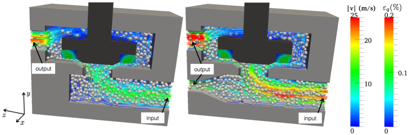
Figure 1: Pressure valve (left) and safety valve (right) setups with particles (silver), fluid stream lines (colored according to fluid speed $|v|\ (m/s)$), deformable solid (colored according to equivalent shear strain $\varepsilon_{q}$), valve (dark gray), and frame (light gray). A spring (not shown) applies a downward force on the valve.

In testing our method, we provide numerical validations of the new techniques introduced. We also perform validations of the LBM approach in the simulated valve geometry. In analyzing valve simulation results, we provide physical commentary where possible to justify various observations.

2 Numerical method

The discrete-element method (DEM) is already a mature tool that is applied in conjunction with experiments both for a better understanding of the micromechanics of granular materials and as a means of $virtual$ experimentation when laboratory experiments are unavailable. In a similar vein, the inclusion of a fluid at the subgranular scale in DEM simulations provides a powerful tool in the broad field of fluid-grain mixtures. Obviously, the available computational power and research time restrict considerably the number of particles or the size of a physical system.

In the case of dry granular materials, statistically representative samples are obtained and simulated with $O(10^{4})$ of particles in 2D Voivret2007 . Despite enhanced kinematic constraints, 2D simulations often lead to novel physical insights and realistic behaviors that can be easily generalized to 3D configurations. However, with fluid in the pore space, 2D simulations are much less reliable in the dense regime since the pore space is discontinuous with zero permeability. This two-dimensional flaw can be partially repaired by adding artificially a permeable layer on the particles. But only 3D simulations may account for a realistic behavior of particle-fluid mixtures with their natural permeability. Moreover, complex geometries/boundaries relating to realistic engineering problems cannot be fully captured in 2D simulations or symmetric 2D extensions (e.g. axis-symmetry); only 3D approaches can handle such problems in full generality.

We developed a 3D fluid dynamics algorithm based on the lattice Boltzmann method (LBM). This algorithm was interfaced with a DEM algorithm with a standard linear spring-dashpot-friction model of contact between particles. The combined LBM-DEM method for particle-laden fluid is then further coupled to a deformable solid domain using finite elements to model a rubber-like behavior. The rubber coupling is intentionally simplified.

Within actual computer power, it is still a significant challenge to model the entirety of most engineering systems and problems. Certain sub-scale details and complex interactions are unnecessary to capture the macroscale system response for a given loading. We utilize symmetric boundaries (where possible) and a variety of techniques to shrink the system size and average-up sub-scale phenomena. Specifically in this work: to handle sub-scale behavior in the fluid we use a Large-Eddy-Simulation (LES) technique (see Sect. 2.2), to mimic a large fluid domain outside the focus region we have created a technique we denote Zoom-in with Effective Boundaries (ZIEB) (see Sect. 2.6), and to reduce simulation time we developed a weak coupling to the rubber domain based on a Neo-Hookean model developed in Abaqus. The last part is computed separately and only the result is imported into LBM-DEM simulation; the coupling and description of this part is expounded in Sec. 2.4.

2.1 Discrete-element method

The DEM is based on the assumption of elastic solids with damping and frictional contact behavior Cundall1971 ; Allen1987 ; Jean1999 ; Moreau1993 ; Luding1996 ; Luding2008 ; Radjai2009 ; Brilliantov2002 . Newton’s equations of motion are integrated for all degrees of freedom with simple force laws expressing the normal and friction forces as explicit functions of the elastic deflection defined from the relative positions and displacements at contact points. We treat all quasi-rigid solids in the domain using this DEM description, including grains, the valve, and solid system boundaries. Correspondingly, all solid-on-solid contact forces (e.g. grain on grain, grains on valve, grain on solid wall) are obtained using DEM contact laws. The valve and system walls are discretized as a kinematically constrained connected mesh of polyhedral solid ‘particles’.

To simplify contact interactions, we assume linear elastic normal and tangential contact forces characterized by a normal stiffness $k_{n}$ and tangential stiffness $k_{t}$. This is applied to all contact interactions, e.g. between spheres, polyhedra, or sphere-polyhedra, though the stiffnesses can vary depending on the two objects in contact. In additional to the elastic part, a dissipative part of the contact force is necessary Moreau1993 ; Luding2008 ; Hart_1988 ; Walton_1993 . In our model, we use a linear visco-elastic law for normal damping and a linear visco-elasto-plastic law for tangential damping and friction forces where the plastic part uses a Coulomb law. The visco-elastic law is modeled by a parallel spring-dashpot model. The contact normal force is defined as:

$$\mbox{f\ }^{n}=\left\{\begin{array}[]{ll}k_{n}-\gamma_{n}\ \vec{v}^{r}_{n}\cdot\vec{n}&\mbox{ if}\ \delta_{n}\leq 0\\ 0&\mbox{ otherwise}\end{array}\right.$$ (1)

where $\vec{n}$ is the contact normal vector and $\vec{v}^{r}_{n}$ is the relative velocity along the contact normal. $\gamma_{n}$ represents a viscosity parameter with a value that depends on the normal restitution coefficient between grains. According to Coulomb’s law the friction force is given by:

$$\vec{f\ }^{t}=\left\{\begin{array}[]{ll}k_{t}{\vec{\delta}}_{t}\ -\gamma_{t}\ \vec{v}^{r}_{t}&\mbox{ if}\ \ |\vec{f\ }^{t}|\leq\mu_{s}\mbox{f}^{n}\\ -\mu_{s}f_{n}\frac{{\vec{v}}^{r}_{t}}{|{\vec{v}}^{r}_{t}|}&\mbox{ otherwise}\end{array}\right.$$ (2)

and

$$\vec{\delta}_{t}=\left\{\begin{array}[]{ll}\int_{t}\vec{v}^{r}_{t}dt&\mbox{ if}\ \ |\vec{f\ }^{t}|\leq\mu_{s}\mbox{f}^{n}\\ \\ \frac{1}{k_{t}}\vec{f\ }^{t}&\mbox{ otherwise}\end{array}\right.$$ (3)

where $\mu_{s}$ is the friction coefficient, ${\vec{v}}^{r}_{t}={\vec{v}}^{r}-{\vec{v}}^{r}_{n}$ is the tangential relative velocity, and $\gamma_{t}$ is a viscosity parameter, which depends on the tangential restitution coefficient.

The equations of motion (both linear and angular momentum balance) are integrated according to a Velocity Verlet scheme Allen1987 .

2.2 Lattice Boltzmann method

The LBM is based on a material representation of fluids as consisting of particle distributions moving and colliding on a lattice Bouzidi2001 ; Feng2007 ; Feng2004 ; Yu:2007aa . The partial distribution functions $f_{i}(\vec{r},t)$ are introduced to represent the probability density of a fluid particle at the position $\vec{r}$ with a velocity $\vec{u}=\vec{c_{i}}$ at time $t$ along discrete direction $i$. The three components of $\vec{c_{i}}$ are given in Tab. 1.

Table 1: The $\vec{c_{i}}$ components for a $D3Q19$ scheme (see Fig. 2).

$i$	0	1	2	3	4	5	6	7	8	9	10	11	12	13	14	15	16	17	18
$x$	0	-1	0	0	-1	-1	-1	-1	0	0	1	0	0	1	1	1	1	0	0
$y$	0	0	-1	0	-1	1	0	0	-1	-1	0	1	0	1	-1	0	0	1	1
$z$	0	0	0	-1	0	0	-1	1	-1	1	0	0	1	0	0	1	-1	1	-1

The Lattice Boltzmann method is often non-dimensionalized when applied to physical problems. The governing macroscopic equations are given in terms of lattice units:

$$\begin{array}[]{lr}\mbox{Characteristic length scale}&\Delta x\\ \mbox{Characteristic velocity}&c\\ \mbox{Characteristic density}&\rho_{{}_{f}}\\ \end{array}$$ (4)

where $\Delta x$ is the lattice spacing, $c=\Delta x/\Delta t$ is the lattice speed with $\Delta t$ the time step, and $\rho_{{}_{f}}$ is the fluid density at zero pressure. For the following, we will describe the method in lattice units.

Figure 2 shows a cartesian grid where the meshing scheme D3Q19, corresponding to 18 space directions in 3D used in our simulations, is represented. In LBM, the scheme D3Q19 is defined for each node where the distribution functions evolve according to a set of rules, which are constructed so as to ensure the conservation equations of mass, momentum and energy (with dissipation), so as to recover the Navier-Stokes equations He:1997aa . This holds only when the wave lengths are small compared to the lattice spacing Chapman:1970aa .

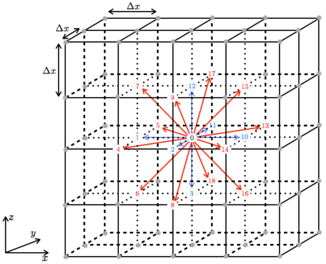
Figure 2: 3D lattice discretization with 18 directions (D3Q19).

At each lattice node, the fluid density $\rho$ and momentum density $\rho\vec{u}$ are defined as

$$\rho=\sum_{i}f_{i}.$$ (5)

$$\rho\vec{u}=\sum_{i}f_{i}\vec{c_{i}}.$$ (6)

and the temperature is given by

$$\frac{D}{2}kT=\sum_{i}\frac{1}{2}m(\vec{c_{i}}-\vec{u})^{2}\frac{f_{i}}{\rho}$$ (7)

where $D$ is the number of space dimensions, $m$ is particle mass, and $k$ is the Boltzmann constant. The equilibrium state is assumed to be governed by the Maxwell distribution:

$$f^{eq}(\vec{c})=\rho\left(\frac{m}{2\pi kT}\right)^{D/2}\exp\left[-\frac{m}{2kT}(\vec{c}-\vec{u}){}^{2}\right]$$ (8)

where $\vec{u}$ is the mean velocity. By expanding (Eq. 8) to order 2 as a function of $u/c_{s}$, which is the local Mach number with $c_{s}$ being the LBM sound velocity, a discretized form of the Maxwell distribution is obtained and used in the LBM:

$$f_{i}^{eq}=\rho w_{i}\left[1+\frac{\vec{c_{i}}\cdot\vec{u}}{c_{s}^{2}}-\frac{u^{2}}{2c_{s}^{2}}+\frac{(\vec{c_{i}}\cdot\vec{u})^{2}}{2c_{s}^{4}}\right]$$ (9)

where the factor $w_{0}=1/3$, $w_{(1,2,3,10,11,12)}=1/18$ and the rest of $w_{i}=1/36$. $w_{i}$ depend on the scheme with the requirement of rotational invariance Satoh:2011aa . The LBM sound speed is then given by $c_{s}=\sum_{i}w_{i}c_{i}^{2}=1/\sqrt{3}$.

The velocities evolve according to the Boltzmann equation. In its discretized form, it requires an explicit expression of the collision term. We used the Bhatnagar-Gross-Krook (BGK) model in which the collision term for each direction $i$ is simply proportional to the distance from the Maxwell distribution Bathnagar:1954aa :

$$\frac{\partial f_{i}}{\partial t}_{coll}=\frac{1}{\tau}\left(f_{i}^{eq}(\vec{r},t)-f_{i}(\vec{r},t)\right)$$ (10)

where $\tau$ is a characteristic time. Hence, for the D3Q19 scheme, we have a system of $18$ discrete equations governing the distribution functions:

$$f_{i}(\vec{r}+\vec{c_{i}}\Delta t,t+\Delta t)=f_{i}(\vec{r},t)+\mbox{$\frac{1}{\tau}$}\left(f_{i}^{eq}(\vec{x},t)-f_{i}(\vec{r},t)\right)$$ (11)

These equations are solved in two steps. In the collision step, the variations of the distribution functions are calculated from the collisions:

$$\tilde{f}_{i}(\vec{r},t+\Delta t)=f_{i}(\vec{r},t)+\mbox{$\frac{1}{\tau}$}\left(f_{i}^{eq}(\vec{r},t)-f_{i}(\vec{r},t)\right)$$ (12)

where the functions $\tilde{f}_{i}$ designate the post-collision functions. In the streaming step, the new distributions are advected in the directions of their propagation velocities:

$$f_{i}(\vec{r}+\vec{c_{i}}\Delta t,t+\Delta t)=\tilde{f}_{i}(\vec{r},t+\Delta t).$$ (13)

The above equations imply an equation of state Chapman:1970aa ; Chen1998 ; He1997 :

$$P(\rho)=\rho c_{s}^{2}.$$ (14)

The kinematic viscosity is then given by Guo2000 ; He1997

$$\eta=c_{s}^{2}\left[\tau-\frac{1}{2}\right]$$ (15)

with the requirement $\tau>1/2$.

As discussed in Chapman:1970aa , the Lattice Boltzmann method holds only when the pressure wave lengths are small compared to the lattice spacing unit. This imposes a limitation on Mach number $Ma=u/c_{s}\ll 1$ and therefore fluid speeds higher than the sound speed cannot be simulated.

In nature, for a given fluid we have: sound speed $c*c_{s}$, density $\rho_{{}_{f}}$ and viscosity $\eta_{{}_{f}}$. From Eq. 12, we need the relaxation time $\tau$. This is related to $c$, $\eta_{{}_{f}}$ and $\Delta x$ by:

$$\tau=0.5+\frac{\eta_{{}_{f}}}{c_{s}^{2}}\frac{1}{c\Delta x}$$ (16)

Equation. 16 shows that since $c$ and $\eta_{{}_{f}}$ are fixed from fluid properties, only $\Delta x$ can be used to ensure the stability of LBM, which becomes unstable when $\tau\rightarrow 1/2$. Numerically, there is a limitation in computer capability regarding the smallest value of $\Delta x$. To handle this, a sub-grid turbulent model based on LES with a Smagorinsky turbulence model is used Yu2005 ; kraichnan1976 ; Smaqorinsky1963 ; Moin1982 . The viscosity formulation is:

$$\eta^{*}=\eta+\eta_{{}_{t}}=c_{s}^{2}\left[\tau^{*}-\frac{1}{2}\right]=c_{s}^{2}\left[\tau+\tau_{{}_{t}}-\frac{1}{2}\right]$$ (17)

where $\eta_{{}_{t}}=c_{s}^{2}\tau_{{}_{t}}$ is the sub-grid LES viscosity and $\tau_{{}_{t}}$ is the sub-grid LES LBM relaxation time. The LES viscosity is calculated from the filtered strain rate tensor $S_{\alpha,\beta}=\frac{1}{2}\left(\partial_{\alpha}u_{\beta}+\partial_{\beta}u_{\alpha}\right)$ and a filter length scale $l_{x}$ through the relation $\eta_{{}_{t}}=\left(Cl_{x}\right)^{2}S$ where $C$ is the Smagorinsky constant. In LBM, $S$ is obtained from the second momentum hou1996 $\Pi_{\alpha,\beta}=\sum_{i\neq 0}c_{i\alpha}c_{i\beta}(f_{i}-f_{i}^{eq})$ as $S=\frac{\Pi}{2\rho c^{2}_{s}\tau^{*}}$, where $\Pi=\sqrt{2\Pi_{\alpha,\beta}\Pi_{\alpha,\beta}}$. From $S$ and $\Pi$, $\tau_{{}_{t}}$ is expressed as:

$$\tau_{{}_{t}}=\frac{1}{2}\left[\sqrt{\tau^{2}+2\sqrt{2}(Cl_{x})^{2}\left(\rho c^{4}_{s}\delta t\right)^{-1}\Pi}-\tau\right]$$ (18)

where the filter length scale $l_{x}=\Delta x$ is the spatial lattice discretization.

2.3 LBM-DEM coupling

There exist different techniques to model fluid-structure interaction. The most used in CFD is stress integration, however, in LBM the preferred approach is based on momentum exchange Bouzidi2001 ; Feng2007 ; Iglberger2008 ; Yu2003 ; Li2004 ; Peskin_1972 ; Wan_2006 ; Wan_2007 . This approach is simple in LBM, since in LBM each node already contains information about the derivatives of the hydrodynamic variables in each distribution function $f_{i}$ Chen1998 . Due to the presence of a solid boundary, after the collision step but before the streaming step, we know the population of $f_{i}$ except those which reflect off the solid wall as shown in Fig. 3 ($f_{i}=?$). In our simulations, we use the method developed by Bouzidi Bouzidi2001 , which mimics a macroscopic no-slip condition. For clarity, we describe the interaction rules using lattice units. This means that the time step is $one$, the space discretization is $one$, etc. Out of the characteristic scales, we will denote, around the fluid-solid boundary, $x$ as position and the subscripts $f$, $s$, and $b$ respectively will indicate either the fluid or solid domain and the fluid-solid boundary. We present the method in simplified 1D form. For more clarity in the way momenta are exchanged between fluid and solid domains, let us introduce $q=|x_{b}-x_{f}|/\Delta x$. According to the LBM scheme (collide and stream Sect. 2.2) in the presence of a solid wall, we have two scenarios depending on the wall position $x_{b}$ (see Fig. 3):

1. $q<\frac{1}{2}$ where fluid leaves node $x_{f}$, reflects off the wall, and reaches $x_{f}$ again in time less than $\Delta t$.

2. $q\geq\frac{1}{2}$ where fluid leaves node $x_{f}$, reflects off the wall, and reaches $x_{f}$ again in time greater than $\Delta t$.

To handle these scenarios, we introduce a fictitious node $x_{f}^{\prime}$(see Fig. 3) such that after streaming, a fluid particle leaving $x_{f}^{\prime}$ arrives at $x_{f}$ exactly in time $\Delta t$.

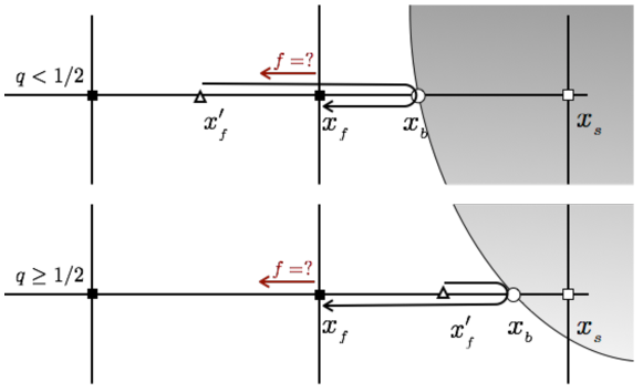
Figure 3: A 2D illustration of the fluid-structure interaction scheme. Black squares are fluid nodes, triangles are fictitious nodes, empty squares are solid nodes and circles are boundary nodes.

As shown in Fig. 3, if $x_{f}$ is the last fluid node before we reach the solid boundary, $x_{s}=x_{f}+c$ should be a solid node. Let $f_{i^{\prime}}$ be the distribution function such that $f_{i^{\prime}}$ is the opposite direction of $i$ where $i$ is the direction oriented from fluid node to solid boundary. By using a linear interpolation, $f_{i^{\prime}}$ is expressed as follow:

$$\begin{array}[]{lcr}f_{i^{\prime}}(x_{f},t+\Delta t)=2qf_{i}^{c}(x_{f},t)+(1-2q)f_{i}^{c}(x_{f}-\vec{c}_{i},t)+\partial f_{i^{\prime}}^{w}&\ \mbox{ for}&q<\frac{1}{2}\\ f_{i^{\prime}}(x_{f},t+\Delta t)=\frac{1}{2q}f_{i}^{c}(x_{f},t)+\frac{2q-1}{2q}f_{i}^{c}(x_{f}+\vec{c}_{i},t)+\partial f_{i^{\prime}}^{w}&\ \mbox{ for}&q\geq\frac{1}{2}\end{array}$$ (19)

where $f_{i}^{c}$ corresponds to the distribution function of $f_{i}$ after the collision step but before streaming and $f_{i}^{c}(x_{f}+\vec{c}_{i},t)=f_{i^{\prime}}^{c}(x_{f},t)$. The term $\partial f_{i^{\prime}}^{w}$ is calculated from the boundary velocity and is zero if the boundary is stationary. $\partial f_{i^{\prime}}^{w}$ is calculated by considering that the fluid velocity $u$ evolves linearly between $x_{f}$ and $x_{s}$. If $u_{0}$ is the boundary velocity, $u$ is then defined by

$$u=u_{0}+(x_{f}-q)\frac{\partial u}{\partial x}$$ (20)

at first order in $u$. The equilibrium value of $f_{i}$ is given by $f_{i}=f_{i}^{0}+3\omega_{i}u\cdot c_{i}$ where $f_{i}^{0}$ is constant and depends on the lattice discretization scheme Bouzidi2001 ; Ladd2001 . Using a linear interpolation, $\partial f_{i^{\prime}}^{w}$ is given by:

$$\begin{array}[]{lcr}\partial f_{i^{\prime}}^{w}=6\omega_{i}\ u_{0}\ c_{i}&\ \mbox{ for}&q<\frac{1}{2}\\ \partial f_{i^{\prime}}^{w}=\frac{3}{q}\omega_{i}\ u_{0}\ c_{i}&\ \mbox{ for}&q\geq\frac{1}{2}\end{array}$$ (21)

Hydrodynamic forces acting on the structure are calculated by using momentum exchange Bouzidi2001 ; Iglberger2008 ; Yu2003 ; Lallemand2003 . Let $\vec{Q}_{f}$ and $\vec{Q}_{s}$ be fluid and solid momentum calculated near the boundary. The exchanged momentum is given by:

$$\Delta\vec{Q}=\vec{Q}_{s}-\vec{Q}_{f}.$$ (22)

$\vec{Q}_{f}$ and $\vec{Q}_{s}$ are calculated as follows:

$$\vec{Q}_{f}=\Delta x^{D}\sum_{all}\sum_{i}f_{i}^{f}\vec{c}_{i}$$ (23)

$$\vec{Q}_{s}=\Delta x^{D}\sum_{all}\sum_{i}f_{i^{\prime}}^{s}\vec{c}_{i^{\prime}}$$ (24)

where $D$ is the space dimension, and $f_{i}^{f}$ and $f_{i^{\prime}}^{s}$ are respectively the fluid and the solid distribution functions. To be clear, $f_{i^{\prime}}^{s}$ is constructed at a lattice point occupied by solid by taking the solid velocity $\vec{u}_{s}$ and density $\rho_{s}$ and assigning a Maxwell equilibrium distribution, per Eq. 9. The hydrodynamic force $\vec{F}$ and torque $\vec{T}$ are then given by:

$$\vec{F}=\frac{\Delta\vec{Q}_{fs}}{\Delta t}=\frac{\Delta x^{D}}{\Delta t}\sum_{all}\sum_{i}(f_{i}^{f}+f_{i^{\prime}}^{s})\vec{c}_{i^{\prime}}$$ (25)

$$\vec{T}=\frac{\Delta x^{D}}{\Delta t}\sum_{all}\sum_{i}l\times(f_{i}^{f}+f_{i^{\prime}}^{s})\vec{c}_{i^{\prime}}$$ (26)

where $l$ is the distance between the center-of-mass of the solid domain and the boundary node $x_{b}$.

2.4 LBM-DEM-Rubber coupling

Unlike the coupling between LBM and DEM, the LBM-Rubber and DEM-Rubber coupling is indirect. We focus our explanation below on the case of a rubber ring component of a valve, but the idea can be generalized to other cases.

A first simulation is performed using Abaqus from which the deformed rubber shape and reaction force of the valve seat on the rubber are saved for many states of rubber compression. This simulation uses no fluid or particles. The Abaqus simulation consists of compressing the rubber ring geometry against the bare valve seat (see inset of Fig. 5). The rubber is simulated as a nearly incompressible neo-Hookean elastic solid with a strain energy $\Psi$ (per unit reference volume) given by $\Psi=(G_{r}/2)\left(\overline{I}_{1}-3\right)+(K_{r}/2)\left(J-1\right)^{2}$ where $\overline{I}_{1}$ is the first deviatoric strain invariant defined as $\overline{I}_{1}=\overline{\lambda}_{1}^{2}+\overline{\lambda}_{2}^{2}+\overline{\lambda}_{3}^{2}$, the deviatoric stretches are given by $\overline{\lambda}_{i}=J^{\frac{1}{3}}\lambda_{i}$, $J$ is the total volume ratio, and $\lambda_{i}$ are the principal stretches. The (small-strain) shear modulus is $G_{r}$ and bulk modulus is $K_{r}$. A frictionless contact between rubber and valve seat is used for simplicity. Figure 4 shows several snapshots during the Abaqus simulation and Fig. 5 gives the seat net-force on rubber as a function of (downward) displacement $\delta$ of the rubber ring, $h(\delta)$. We index each deformed rubber configuration by the value of $\delta$ it corresponds to. The Abaqus tests are performed under quasi-static conditions but we also assume damping can exist such that upward the force on the rubber satisfies the relation

$$F=h(\delta)+\nu\dot{\delta}.$$ (27)

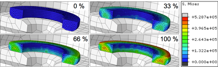
Figure 4: Snapshots of rubber deformation during the Abaqus simulation at 0 %, 33 %, 66 % and 100 % of the simulation duration where the color map shows the Mises stress in Pa.

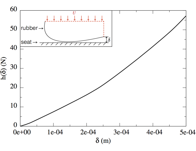
Figure 5: Net-force of valve seat on rubber as function of displacement. The inset shows the configuration of Abaqus simulation where the dot line represent the imposed velocity boundary $U$.

Then, the data from the Abaqus simulation is used in a weak coupling routine to describe rubber configurations when the ring takes part in a slurry simulation. In short, the method determines which of the deformed rubber configurations from the stand-alone Abaqus tests is the best representation of the actual deformed rubber state at that moment in the slurry problem. Hence, the utility of this method lies in the fact that the rubber deformation that occurs in the actual slurry problem largely resembles the modes of deformation seen in a purely solid compression experiment. Situations where the rubber surface becomes heavily locally deformed could be problematic for this approach.

From the LBM-DEM point of view, the rubber is composed of tetrahedra; this allows us to compute contact forces for DEM and the exchanged momentum for LBM as if it were a simple collection of polyhedral objects. Since the Abaqus simulation is performed without fluid or particles, to use its solutions we need to deduce an effective upward force from LBM-DEM acting on the bottom rubber surface, which can then be referenced against the Abaqus data to infer a deformed rubber shape. The effective force is needed because the rubber in the Abaqus simulations has contact only with the valve seat, whereas in the slurry case, there can be additional forces from fluid and particles extending to the lateral surfaces of the rubber.

Key to our routine is to identify two subsets of the exposed rubber surface, denoted surface A and surface B. Surface A is the part that makes contact with the valve seat and surface B remains free in the Abaqus simulations (see left Fig .6). In particular, surface $A$ and $B$ are geometrically defined using the the last frame of the Abaqus simulation where the rubber is fully compressed. In the slurry case, we add uniform hydrostatic stress to the observed rubber loading distribution until the mean normal stress acting on surface B vanishes. This leaves us with a loading state that resembles one from Abaqus. Because the rubber is essentially incompressible, changing the hydrostatic stress uniformly along the surface does not affect the deformed rubber configuration. To be specific, we compute the normal stress on surface $A$ using $P_{{}_{A}}=\frac{1}{A}\int_{A}\vec{n}\cdot\vec{f}dS$ and on surface $B$ using $P_{{}_{B}}=\frac{1}{B}\int_{B}\vec{n}\cdot\vec{f}dS$ where $\vec{f}$ is the stress from hydrodynamic, particle, and valve-seat forces and $\vec{n}$ is the normal vector on section $dS$. Since the rubber deformation is caused by the shear part of the stress, we uniformly subtract the traction $P_{{}_{B}}$ from all normal stresses acting on the rubber. This modified loading now resembles the Abaqus loading (inset Fig. 5) in which only an upward force on surface $A$ exists. Therefore, we define the effective upward force on surface $A$ as ${F}=\text{Area}_{A}\cdot(P_{{}_{A}}-P_{{}_{B}})$.

The rubber shape is updated using a four step loop, which is performed after particle positions and fluid data are updated. The goal of the iteration routine is to implicitly solve Eq. 27 for $\delta$ so that the effective force from particles, fluid, and the valve seat on the final rubber state matches the force from Eq. 27.

• Step 1: Compute effective upward force $F$ from fluid, particle, and valve-seat interactions on rubber given the current guess for $\delta$

• Step 2: Use this force and Eq. 27 to update to a new guess for $\delta$.

• Step 3: Check if new and old $\delta$ differ by less than a tolerance. If so break, if not update the rubber shape based on the new $\delta$.

• Step 4: Update applied force on surfaces $A$ and $B$ according to the rubber shape given by the new guess for $\delta$.

We assume that fluid forces do not change throughout the iteration procedure. This is true by assuming a small incremental rubber shape change between iterates, so only particle and valve-seat forces on the rubber are updated during Step 4.

In Step 2 we utilize the following update rule

$$\delta\leftarrow\frac{\left[F-h(\delta)+\delta_{0}\frac{\nu}{\Delta t}\right]\frac{\Delta t}{\eta}+\delta}{1+\frac{\nu}{\eta}}$$ (28)

where $\delta_{0}$ is the actual displacement of the rubber at the beginning of the time-step. The coefficient $\eta$ is numerically selected to aid convergence. Note that if the updated value of $\delta$ matches the value inputted, then Eq. 27 is solved. The update rule above attempts to move $\delta$ toward such a solution with each pass through the iteration loop. We check convergence of $\delta$ (Step 3) using a tolerance that is scaled by the error of the first iterate, $\delta_{1}-\delta_{0}$, where $\delta_{1}$ is the value obtained for $\delta$ after the first pass of the loop.

We use simple linear interpolation to compute values of $h(\delta)$ when $\delta$ is between two neighboring values from the Abaqus output.

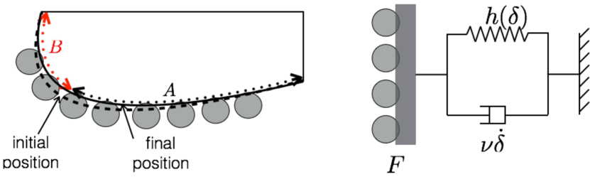
Figure 6: Configuration of rubber-LBM-DEM coupling. The left figure gives the geometrical definitions of area $A$ and $B$, and the initial and final shape of the rubber as it proceeds through the iteration loop to solve Eq. 27, with a representation of particles in contact shown. The right figure gives a 1D analog of the model to compute the rubber deformation.

The third step consists of updating the rubber shape using the new guess for $\delta$ obtained in Step 2. Again, a linear interpolation is applied as is done for $h(\delta)$. For the shape, we export the Abaqus mesh, which allows the interpolation. For example, if the new $\delta$ lies directly between two frames of the Abaqus data, the rubber shape is updated by moving the nodes of the rubber to positions halfway between those of the neighboring frames.

The fourth step consists of recomputing the contact force between the tetrahedra representing the rubber, and the particles/valve-seat. The contact force is computed using Eq. 1 for the normal part and Eq. 2 for the tangential part. One specificity here is that we do not update $\vec{\delta_{t}}$ during the coupling loop routine unless when $|\vec{f\ }^{t}|>\mu_{s}\mbox{f}^{n}$ where $\vec{\delta_{t}}=\frac{1}{k_{t}}\vec{f\ }^{t}$. A schematic model of one update through the iteration loop is presented in Fig. 6 (left) and a 1D mechanical model of the treatment of the rubber interaction is visualized in Fig. 6 (right).

2.5 Numerical algorithm

The numerical method described in previous sections is implemented using the algorithm displayed in Fig. 7. Note that we compute the valve acceleration by enjoining the applied force and mass of the rubber and valve components together in the Verlet update; rubber deformations are not included in the calculation of net acceleration of the valve/rubber composite as they are small compared to the movement of the valve overall. As shown in Fig. 7, the LBM step is computed in parallel with DEM force calculation and Rubber force calculation.

Figure 7: LBM-DEM-RUBBER implementation algorithm.

2.6 Zoom-in with Effective Boundaries (ZIEB)

The Zoom-In with Effective Boundaries (ZIEB) technique replaces a fluid reservoir/domain with an analytical solution that interacts dynamically with the remainder of the domain. The challenge is to determine the correct effective dynamics at the fictitious interface, and to transfer the analytical result to LBM distribution functions. In this study we model valves, which can be positioned far from the pump that leads the slurry to the valve. The goal is to avoid having to calculate flow in the expansive pump region. From a computational point of view, one might assume a simple input velocity boundary condition should solve the problem, however, for a compressible fluid, the imposed flow and pressure may depend on the total removed volume and feedback with the dynamics within the valve system. In this section, we first detail how to obtain the analytical solution then explain how to implement this solution as an LBM boundary condition.

ZIEB analytical solution

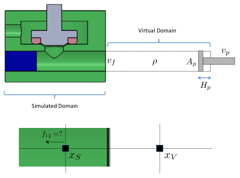
Figure 8: Top: Full geometry of problem to be solved — valve region connected to a cylinder and piston region. ZIEB technique allows removal of the piston/cylinder domain from the simulation, by replacing it with effective boundary conditions at the fictitious interface. Bottom: Zoom-in near the fictitious interface showing the first simulated lattice point (at $x_{S}$) and the closest virtual lattice point (at $x_{V}$).

Per Fig. 8, we assume the virtual (i.e. removed) domain is a cylinder and piston. The cylinder is initially full of fluid and has total volume $V_{0}$. As the piston moves, fluid is pushed into the simulated domain. Let the movement of the piston be given by some prescribed $H_{p}(t)$, where $H_{p}$ measures the piston displacement. The cross-sectional area of the piston (and cylindrical domain) is $A_{p}$. The piston velocity, $v_{p}(t)$, is simply defined from the time-derivative of $H_{p}$. Define as $v_{f}$ the mean in-flowing fluid velocity component on the interface between the domains. Let $\rho$ be the average density of fluid in the virtual cylinder between the piston head and the interface. Further, we make the simplifying assumption that in the cylinder region the fluid density is in fact uniform, such that it is equal to $\rho$ throughout.

Conservation of fluid mass in the cylinder domain can be expressed by balancing the mass rate within the cylinder against the mass flux into the simulated domain:

$$\frac{d}{dt}\rho\cdot(V_{0}-A_{p}H_{p})=-\rho v_{f}A_{p}\ \ \Rightarrow\ \ \frac{d\rho}{dt}=\rho\left[\frac{v_{p}A_{p}-v_{f}A_{p}}{V_{0}-A_{p}H_{p}}\right]$$ (29)

In a fully continuum framework, the above equation would need to be augmented with momentum balance in order to provide the in-flowing velocity, $v_{f}$, at the fictitious interface. However, using the LBM description, we can update $v_{f}$ in another way, which is consistent with momentum balance on the small scale.

Implementation of ZIEB analytical solution in LBM

At a given time $t^{n}$, we assume $\rho^{n}$ is given in the cylinder domain and is equal to the density at $x_{S}$, where, per Fig. 8, $x_{S}$ is the lattice point in the simulated domain that is adjacent to the interface with the virtual domain. We suppose the velocity at $x_{S}$ is the interfacial velocity $v_{f}^{n}$. Both density and velocity at time $t^{n}$ at $x_{S}$ are defined by Eq. 5 and 6 through distribution functions $f_{i}^{n}$.

The distribution functions are updated to $t^{n+1}$ under the following procedure, which is applied after the collision step but before streaming. First we update and store the density $\rho^{n+1}$ at $x_{S}$ using explicit integration of Eq. 29:

$$\rho^{n+1}=\rho^{n}\exp\left[\frac{v_{p}^{n}A_{p}-v_{f}^{n}A_{p}}{V_{0}-A_{p}H^{n}_{p}}\Delta t\right]$$ (30)

Next, a partial LBM streaming step is performed at $x_{S}$ using the distributions at time $t^{n}$. During this step $x_{S}$ streams to and from its neighboring ‘real’ lattice points within the simulated domain. However, it only streams out of the interface with the virtual domain and does not receive any distributions from the virtual domain. Define $\rho^{*}$ as the density at $x_{S}$ after this partial streaming step.

The next step is to back-solve the needed distributions to be streamed in from the virtual domain in order to guarantee the final density at $x_{S}$ equals $\rho^{n+1}$. For example, consider a setup as shown in Fig. 8 and suppose the fictitious interface is normal to the $\hat{z}$ direction (see Fig. 2). After the partial streaming step, updated (though not finalized) distribution values exist for all the $f_{i}$ except for the values associated to $i=7,\ 9,\ 12,\ 15,$ and $17$. These five distribution values are all unknown after the partial streaming step. To compute them, first we modify only the value of the $f_{12}$ distribution, which is the distribution that streams into the simulated domain normal to the fictitious boundary:

$$f_{12}=\rho^{n+1}-(\rho^{*}-f^{n}_{12})$$ (31)

This advects all the missing density at $x_{s}$ from a fictitious node $x_{V}$ (see bottom of Fig. 8). With these distributions, the velocity at time $t^{n+1}$ is computed at $x_{S}$ according to $u=\frac{1}{\rho^{n+1}}\sum f_{i}$. Because the distributions in the $i=7,\ 9,\ 15,$ and $17$ directions are still unknown at this point, the Maxwell equilibrium function Eq. 9 is then used to redistribute all the distributions at $x_{S}$ to a more natural, equilibrium state. This updates all the distributions to their final values, at $t^{n+1}$.

We notice here that the initial value of $\rho$ at the beginning of the simulation should be a normalized value (in lattice units) otherwise an additional step of normalizing by the physical fluid reference density will be necessary before using it in Eq. 29 and Eq. 31.

2.7 Tests and validations

We first test some of the individual components of the routine. In this section, we provide separate numerical validations of the ZIEB technique, the rubber deformation model, and the LBM.

To validate the ZIEB method, we performed an analysis of fluid flow in a geometry comprised of a piston driving fluid passing through a narrow restriction. This flow field is then compared to that obtained using a “virtual piston” in which the domain containing the moving piston is removed and in its place an effective boundary condition from ZIEB is used, see Fig. 9. The real piston begins positioned such that the fluid volume between the piston and input section is $V_{0}$; the same $V_{0}$ is used in Eq. 30 for the virtual piston. We use $V_{0}=1.77\mbox{e-}06\ m^{3}$ and $A_{p}=7.09\ m^{2}$. As input parameters, we use a (pressure-free) fluid density $\rho_{{}_{f}}=1000\ kg/m^{3}$, dynamic viscosity $\eta=0.001\ Pa.s$ and a Smagorinsky constant of $C=0.4$ for the sub-grid turbulence model Feng2007 ; hou1994 ; germano1991 . Figure 10 shows the comparison between the two simulations regarding fluid velocity and the normalized input fluid density computed in the same domain (see Fig. 9). The agreement is strong, even the time-dependent fluctuations, confirming the correctness of the ZIEB method.

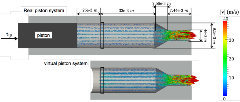
Figure 9: Configuration of tests for the Zoom-in with Effective Boundaries (ZIEB) technique. The real piston geometry is displayed in the top figure (mid-simulation) and the virtual piston geometry is displayed beneath, where ZIEB has been applied on the left boundary to mimic the removed piston domain.

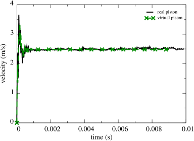
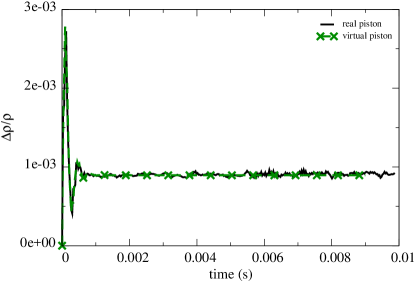
Figure 10: Velocity and normalized input fluid density as functions of time for the real and virtual piston setups. The velocity and density are calculated within the boxed subdomain in Fig. 9.

The test of the rubber coupling and rubber deformation is performed running a loading/unloading test without fluid. A force (loading/unloading) $F_{load}$ is directly applied on the valve which presses the rubber into contact with twelve frozen spheres (see Fig. 11). Two phases are considered: a loading phase with $F_{load}=40\ N$ then an unloading phase with $F_{load}=10\ N$. We use a frictionless contact type between the rubber and spheres where normal stiffness is set to $1\mbox{e+}05\ N/m$ and no normal damping is used to insure that all dissipation comes from internal rubber damping. The rubber coupling parameters (Eq. 28) are set to $\nu=80\ N\cdot s/m$ and $\eta=10\ N\cdot s/m$. The valve density is set to 7850 $kg/m^{3}$ and the rubber density to $1200\ kg/m^{3}$. The time step is set to $1\mbox{e-}07\ s$. Fig. 11 shows the loading/unloading force, the reaction force $F$ of spheres on the rubber, the displacement $\delta$ (right inset) and the corresponding force $h(\delta)$. The agreement of $F_{load}$, $h$, and $F$ after a relaxation time verifies the coupling.

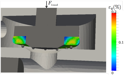
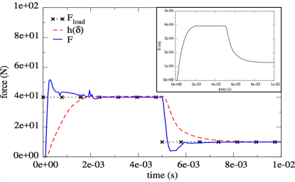
Figure 11: A dry numerical test of the simplified DEM-Rubber coupling. The left figure shows the configuration of the test where the loading/unloading force $F_{load}$ is applied directly to the valve. Color corresponds to equivalent shear strain magnitude $\varepsilon_{q}$ in the rubber. Spheres are held fixed on the valve seat. The right figure shows loading/unloading force $F_{load}$, $h(\delta)$ and the net reaction force $F$ of spheres on rubber. The inset shows the rubber deformation $\delta$ as a function of time.

The last test is focused on verifying the fluid LBM simulation by comparing flow of fluid in the rubber channel of a pressure-valve assembly against an analytical flow solution (recall Fig. 1). We can run a simulation where the fluid viscosity is large, such that the flow in the channel will be in the Stokes limit. To aid in calculating an analytical solution, we treat the flow as radially directed and assert the lubrication approximation. In view of Fig. 1 for the definition of the $y$ direction, we obtain the following system of equations, which includes momentum and mass balance under the lubrication limit:

$$\begin{array}[]{l}\frac{1}{r}\frac{\partial}{\partial r}\left(rv_{r}\right)=0,\ \ \ \frac{\partial p}{\partial y}=0,\\ \eta_{{}_{f}}\frac{\partial^{2}v_{r}}{\partial y^{2}}=\frac{\partial p}{\partial r}.\end{array}$$ (32)

This is solved by $v(r,y)=\frac{A}{r}y(h-y)$ where $A$ is an undetermined constant and $p(r)=-2A\eta_{{}_{f}}\ln(r)+C$ where $C$ is a constant and $A$ is the same as in the velocity field equation. From the $p(r)$ equation, the pressure difference $\Delta p$ between $r=R_{in}$ and outer at $r=R_{out}$ (see Fig. 12) is given by: $\Delta p=-2A\eta_{{}_{f}}\ln(R_{out}/R_{in})$. Using $y=h/2=0.0026\ m$, $R_{in}=0.0065\ m$ and $R_{out}=0.0110\ m$, we find $v(R_{in},h/2)\simeq 4.16\ m/s$ (see Fig. 12 left) from our numerical data, giving $A\sim 1.59\mbox{e+}04\ s^{-1}$. Hence, the predicted pressure difference is $\Delta p\simeq-5.3\mbox{e+}05\ Pa$ which is quite close to the obtained pressure difference from the simulation ($-5.7\mbox{e+}05\ Pa$, see Fig. 12 right). Fig. 13 shows the analytical solution as a function of $r$ in comparison with the numerical data and agreement is found. In this test, the fluid density is $\rho_{{}_{f}}=1000\ kg/m^{3}$ and dynamic viscosity is $\eta_{{}_{f}}=3.16\ Pa\cdot s$. The valve density is set to $7850\ kg/m^{3}$ and the rubber density to $1200\ kg/m^{3}$. We use ZIEB on the input section (see Fig. 14) with a virtual piston velocity of $v_{p}=6\ m/s$, and we apply a constant pressure of $P_{out}=1.04\mbox{e+}04\ Pa$ at the output section (see Fig. 14).

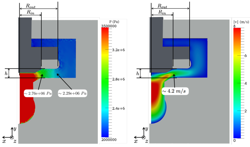
Figure 12: Fluid flow and pressure in the rubber channel. On the left we show the fluid pressure and on the right, the velocity magnitude.

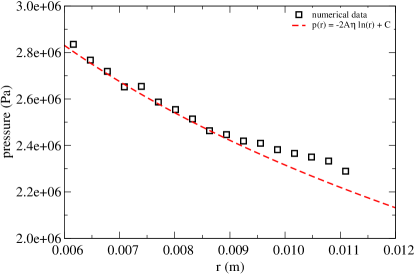
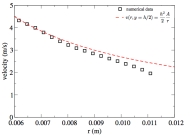
Figure 13: Numerical versus theoretical comparison for pressure (left) and velocity (right) in the rubber channel. $A\sim 1.59\mbox{e+}04\ s^{-1}$, $y=h/2\simeq 0.0013\ m$, $C\sim-2.33\mbox{e+}06\ Pa$.

3 Examples

We present numerical examples utilizing the valve geometries presented in Fig. 14. The two systems are used to mimic a safety and pressure valve. The different parts and their corresponding names are presented in Fig. 14. Their dimensions are given in Appendix A.

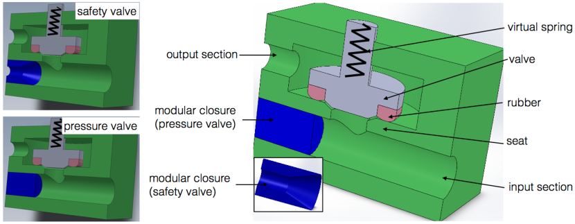
Figure 14: Illustration of different parts of the safety and pressure valve.

The valve is spring-loaded from above. Initially, the valve is closed due to force from the spring (and prescribed overpressure above in the pressure-valve geometry). The spring’s force-displacement relation is chosen to be non-linear and is expressed as follows: $F_{s}=k_{v}\delta_{0}+k_{v}(a/\frac{\pi}{2})\tan(\frac{\pi}{2}\frac{\delta}{a})$; $k_{v}$ is the stiffness, $\delta_{0}=0.092\ m$ is the preload spring displacement, $\delta$ is the load displacement and $a=0.0045\ m$ is the spring maximum compression. The fluid region above the valve begins unpressurized in the safety-valve case and pressurized by the selected $P_{out}$ in the pressure-valve case. For each simulation, both for safety and pressure valve, we start by introducing fluid through the input section beneath valve domain using the ZIEB technique at constant virtual piston velocity $v_{p}$. When the beneath valve domain reaches a large enough pressure, it will overcome the spring-load (and possible top pressure) on the valve to open it. We continue displacing the virtual piston and then turn off $v_{p}$ when we assume that the flow has reached a steady state. We then wait until the valve is closed. We check the behavior of the valve systems with and without particles but the closure phenomena is only investigated for the case where we have particles.

In the presence of particles, we start with a constant packing fraction in the domain beneath the valve corresponding to the imposed packing fraction $\phi$ at the input section. During the simulation, each particle that exits the simulated domain is removed and each new particle introduced at the input section starts with the fluid input velocity as its initial velocity. To control the input particle flow, we insert grains to ensure that the input particle packing fraction is constant within a width of $0.00425\ m$ from the interface with the virtual domain. We introduce/remove particles in the simulated system every 50 steps.

Physical parameters involved in the valve problem are displayed in Tab. 2), which include the geometry of the valve system (e.g. safety-valve or pressure-valve), each of which has fixed size dimensions (see Appendix). For all tests, we fix the solid density of particles $\rho_{{}_{s}}=2500\ kg/m^{3}$, (pressure-free) fluid density $\rho_{f}=1000\ kg/m^{3}$ (small-strain) rubber shear modulus $G_{r}=3.0\mbox{e+}05\ Pa$ and bulk modulus $K_{{}_{r}}=8.0\mbox{e+}06\ Pa$, rubber damping $\nu=80\ N\cdot s/m$, rubber$+$valve mass $M_{{}_{vr}}=9.2\mbox{e-}03\ kg$, and valve spring stiffness $k_{{}_{v}}=625N/m$.

Since mono-disperse particles may induce a crystallisation phenomena at higher packing, a random size distribution is used uniformly between $d_{min}$ and $d_{max}$. The distribution may be described by a mean particle size $d=(d_{min}+d_{max})/2$ and polydispersity $\Delta d=d_{max}/d_{min}$.

Table 2: Parameters.

Particles		Valve + Rubber		Fluid		System
mean diameter	$[d]$	mass	$[M_{{}_{vr}}]$	dynamic viscosity	$[\eta_{{}_{f}}]$	system geometry	$[\text{geo}]$
solid density	$[\rho_{{}_{s}}]$	rubber shear modulus	$[G_{r}]$	pressure-free density	$[\rho_{{}_{f}}]$	system size	$[r]$
polydispersity	$[\Delta d]$	rubber bulk modulus	$[K_{{}_{r}}]$	output pressure	$[P_{out}]$	piston speed	$[v_{p}]$
input packing fraction	$[\phi]$	valve spring stiffness	$[k_{{}_{v}}]$
		rubber damping	$[\nu]$

To generalize the valve dynamics and flow behavior, we choose the natural units of our system to be the input section radius $[L]=r$ for length, time $[T]=\sqrt{\rho_{{}_{f}}r^{3}/k_{{}_{v}}}$ and mass $[M]=\rho_{{}_{f}}r^{3}$. From these units, a dimensionless parametric space is represented by:

$$\left\{\text{geo},\frac{P_{out}}{k_{{}_{v}}},v_{p}\sqrt{\frac{k_{{}_{v}}}{\rho_{{}_{f}}r}},\frac{d}{r},\Delta d,\phi,\frac{\rho_{{}_{s}}}{\rho_{{}_{f}}},\frac{\eta_{{}_{f}}}{k_{{}_{v}}\rho_{{}_{f}}r},\frac{G_{r}r}{k_{{}_{v}}},\frac{K_{r}r}{k_{{}_{v}}},\frac{M_{{}_{vr}}}{\rho_{{}_{f}}r^{3}}\right\}$$

where geo is the system geometry. Taking into account the fixed parameters, the dimensionless parametric space we will explore is described by the following groups:

$$\left\{\text{geo},\frac{P_{out}}{k_{{}_{v}}},v_{p}\sqrt{\frac{k_{{}_{v}}}{\rho_{{}_{f}}r}},\frac{d}{r},\Delta d,\phi,\frac{\eta_{{}_{f}}}{k_{{}_{v}}\rho_{{}_{f}}r}\right\}$$

The second group is only relevant to pressure valves and the latter five can be independently controlled through the selection of $v_{p},d,\Delta d,\phi$, and $\eta_{f}$.

The parameters for all tests are summarized in Tab. 3 and Tab. 4. As indicated in the Tables, the tests are conducted in order to observe the dependence of the valve behavior on each of $\eta_{f},v_{p},d,\Delta d,$ and $\phi$ independently; for each variable, a sequence of tests is performed where it is varied over a range while the others are held fixed.

Table 3: Range of parameters investigated for safety and pressure valve simulations without particles. All units are in $[\text{kg}],[\text{m}],[\text{s}]$.

geo$=$safety valve	geo$=$pressure valve
range fixed $\eta_{{}_{f}}$ 1e-03 to 3.16e+01 name value $P_{out}$ 0 $v_{p}$ 12.5 $d$ 0 $\Delta d$ 0 $\phi$ 0 $v_{p}$ 1 to 12.5 $P_{out}$ 0 $d$ 0 $\Delta d$ 0 $\phi$ 0 $\eta_{{}_{f}}$ 1e-03	range fixed $\eta_{{}_{f}}$ 1e-03 to 3.16e+01 name value $P_{out}$ 10416 $v_{p}$ 6 $d$ 0 $\Delta d$ 0 $\phi$ 0 $v_{p}$ 1 to 12 $P_{out}$ 10416 $d$ 0 $\Delta d$ 0 $\phi$ 0 $\eta_{{}_{f}}$ 1e-03

Table 4: Range of parameters investigated for safety and pressure valve for simulations with particles. All units are in $[\text{kg}],[\text{m}],[\text{s}]$.

geo$=$safety valve	geo$=$pressure valve
range fixed $v_{p}$ 1 to 12.5 $P_{out}$ 0 $d$ 0.8e-03 $\Delta d$ 1.2 $\phi$ 0.084 $\eta_{{}_{f}}$ 1e-03 $d$ 0.8e-03 to 1.5e-03 $P_{out}$ 0 $v_{p}$ 12.5 $\Delta d$ 1.2 $\phi$ 0.053 $\eta_{{}_{f}}$ 1e-03 $\Delta d$ 1.1 to 1.5 $P_{out}$ 0 $v_{p}$ 12.5 $d$ 0.8e-03 $\phi$ 0.053 $\eta_{{}_{f}}$ 1e-03 $\phi$ 0.026 to 0.128 $P_{out}$ 0 $v_{p}$ 12.5 $\Delta d$ 1.2 $d$ 0.8e-03 $\eta_{{}_{f}}$ 1e-03	range fixed $v_{p}$ 1 to 12 $P_{out}$ 10416 $d$ 0.8e-03 $\Delta d$ 1.2 $\phi$ 0.067 $\eta_{{}_{f}}$ 1e-03 $d$ 0.8e-03 to 1.4e-03 $P_{out}$ 10416 $v_{p}$ 6 $\Delta d$ 1.2 $\phi$ 0.053 $\eta_{{}_{f}}$ 1e-03 $\Delta d$ 1.1 to 1.5 $P_{out}$ 10416 $v_{p}$ 6 $d$ 0.8e-03 $\phi$ 0.053 $\eta_{{}_{f}}$ 1e-03 $\phi$ 0.026 to 0.117 $P_{out}$ 10416 $v_{p}$ 6 $\Delta d$ 1.2 $d$ 0.8e-03 $\eta_{{}_{f}}$ 1e-03

The contact model (DEM solver and DEM-Rubber coupling), fluid turbulence model (LES) and numerical parameters are displayed in Tab. 5

Table 5: The contact parameters (DEM solver and DEM-Rubber coupling), fluid turbulence model (LES) and numerical parameters. All units are in $[\text{kg}],[\text{m}],[\text{s}]$.

stiffness	normal	tangantial
seat-valve	1e+11	0
seat-rubber	1e+06	0
seat-particle	1e+07	0.8e+07
valve-particle	1e+07	0.8e+07
rubber-particle	1e+05	0.8e+05
particle-particle	1e+07	0.8e+07

friction coefficient
seat-valve	0
seat-rubber	0
seat-particle	0.4
valve-particle	0.4
rubber-particle	0.4
particle-particle	0.4

damping	normal	tangantial
seat-valve	1e+03	0
seat-rubber	0	0
seat-particle	3	0
valve-particle	3	0
rubber-particle	0	0
particle-particle	3	0

rubber and numerical parameters
Smagorinsky constant	0.4000
lattice speed	2.5e+03
fluid space discretization	3.0e-04
DEM time step	5.0e-08
numerical rubber convergence ($\eta$)	1.0e+01

3.1 Pressure valve lift behavior

In this section, we discuss the effect of fluid viscosity, piston velocity, and input packing fraction on the opening, steady flow, and closure behavior of the valve for a pressure valve configuration. As shown in Tab.  3 and Tab. 4, when varying a parameter of interest, we fix the others to a control set taken from $v_{p}=6\ m/s$, $\eta_{{}_{f}}=0.001\ Pa\cdot s$, $\phi=0.053$ and $\Delta d=1.2$. We will focus our analysis on the pressure valve and will give a brief analysis of the results for the safety valve in Sec. 3.2.

Valve opening phase

During the opening phase, we observe a delay between the initiation of the piston and the initiation of valve opening. The effect is not due to packing fraction Fig. 20 (left), polydispersity Fig. 19 (left) or mean particle diameter Fig. 19 (right), rather, the delay increases with fluid viscosity Fig. 15 (left), and decreases when piston velocity increases Fig. 15 (right) (simulation without particles) and Fig. 20 (right) (simulation with particles). The lack of dependence of the delay time on particle inputs is because the mean particle diameter is bigger than the initial valve lift so it does not modify fluid behavior in the valve-rubber channel (see schematic in Fig. 16). The more dominant effect is negative suction pressure, which develops in the valve-rubber channel as the valve initially displaces upward, as shown in Fig. 17. The delay increases with increasing viscosity because this increases the suction force due to lubrication effects in the narrow valve-rubber channel. At the same time, in the beneath valve region where the fluid domain is not thin, the pressure is mostly independent of viscosity as we observe in Fig. 18 (left) where before the first peak of the valve lift (Fig. 15 (left)) the pressure evolution is the same.

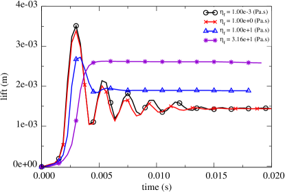
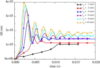
Figure 15: Valve lift as function of time for different fluid viscosity (left) and different virtual piston velocity (right) (without particles).

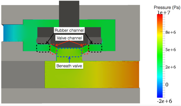
Figure 16: Rubber channel, valve channel, and beneath valve domain configuration.

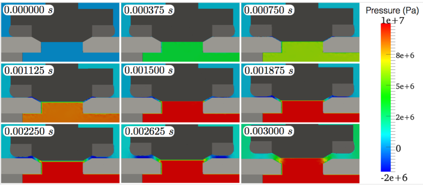
Figure 17: Several snapshots showing valve and rubber channel pressure evolution for $\eta_{{}_{f}}=31.6\ Pas$ and $v_{p}=6\ m/s$. (without particles).

Increasing the piston velocity reduces the delay because the suction pressure in the valve-rubber channel is balanced by faster growth of the beneath valve pressure. Figure 18 (right) shows that during the pressurization phase, the pressure slope increases with piston velocity, as expected.

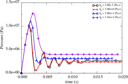
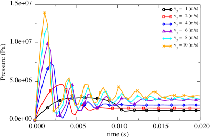
Figure 18: Beneath valve pressure as a function of time for different fluid viscosity (left) and different piston velocity (right) (without particles).

Quasi-steady open valve phase

The valve displacement begins to approach a steady value (with or without oscillations) after the first peak in valve lift ($t\simeq 0.010\ s$) and ends when the piston motion is stopped at $t=0.025\ s$. As shown in Fig. 15, the steady lift position, for the simulations without particles, increases with fluid viscosity and piston velocity. For lower viscosity, the valve has an ‘underdamped’ response characterized by decaying oscillations, whereas for larger viscosities, an ‘overdamped’ response can be seen (see Fig. 15 (left)). The presence of particles can modify the valve lift behavior. Figure 19 (left) shows that virtually no effect on valve lift is observed for different polydispersity in the range we tested. Increasing the mean diameter of particles, Fig. 19 (right), increases the steady lift position but this appears to be primarily a particle size effect; after the initial upward motion of the valve, the valve descends downward and is stopped by a monolayer of mobile particles in the rubber channel, which holds the valve position at roughly $1d$ high. Further tests would be needed at higher fixed piston speeds to determine if the valve positioning depends more robustly on $d$.

Tests involving variation of the packing fraction or the piston velocity, Fig. 20, show a non-trivial valve lift behavior in which three approximate regimes can be identified:

1. A lower input particle flux behavior: $\varphi<\varphi_{{}_{l}}$.

2. A transition input particle flux behavior: $\varphi_{{}_{l}}\leq\varphi\leq\varphi_{{}_{u}}$.

3. A higher input particle flux behavior: $\varphi_{{}_{u}}<\varphi$.

where the input flux is defined by $\varphi=\phi\ v_{p}$.

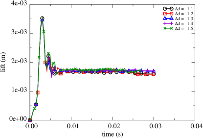
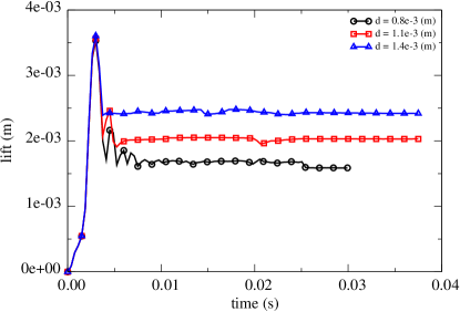
Figure 19: Valve lift as function of time for different polydispersity (left) and different mean grain diameter (right).

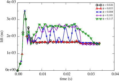
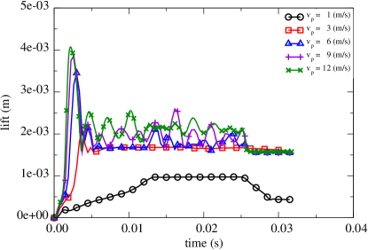
Figure 20: Valve lift as function of time for different packing fraction (left) and different piston velocity (right).

In the first regime, we observe a simple particle suspension flow through the valve and rubber channel with a quasi-constant lift as shown in Fig. 20. The beneath valve packing fraction shows also a quasi-constant value Fig. 21. This regime is observed for $\varphi<\varphi_{{}_{l}}\simeq 0.405$ (from Fig. 20).

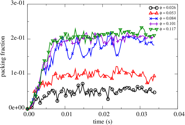
Figure 21: Beneath valve packing fraction as function of time for different input packing fraction.

The second regime is characterized by unsteady motion of the valve that oscillates between notably disparate high and low positions. This regime, for the range of parameters we tested, appears to be limited by $\varphi>\varphi_{{}_{l}}\simeq 0.405$ and $\varphi<\varphi_{{}_{u}}\simeq 0.611$. To better understand the valve lift behavior in this regime let us analyze the lift for $\phi=0.084$. Figure 22 and Fig. 23 show the time dependence of the lift, beneath valve packing fraction, and beneath valve pressure. Notice that the peaks and valleys of the beneath valve pressure and packing fraction are relatively in sync. The peaks in the lift plot are delayed with respect to those of the pressure and packing fraction. This can be understood as follows: when the valve position is low, particles aggregate under the valve and as they do so, they form something of a ‘plug’ that causes the pressure beneath the valve to build up. When the pressure is sufficiently high, the valve will open up to release the pressure, which causes the backed-up grains beneath the valve to escape through the open valve. When this happens it causes the beneath valve packing fraction and the pressure to decrease, which immediately allows the valve to recover to its initial lift (Fig. 22, Fig. 23). This phenomena can be distinguished from the lower input particle flux regime, in that in the lower flux case, the flux of grains into the system is not enough to back-up sufficiently under the valve and induce a pressure build-up.

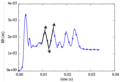
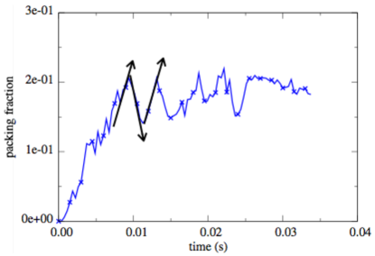
Figure 22: Valve lift (left) and beneath valve packing fraction (right) for $\phi=0.084$ as function of time.

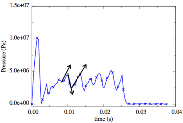
Figure 23: Beneath valve pressure as function of time for $\phi=0.084$.

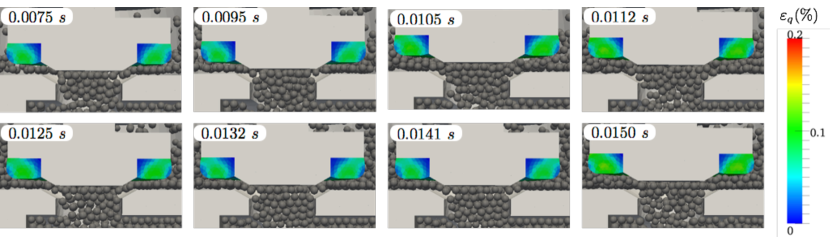
Figure 24: Several snapshots showing particles beneath valve for $\phi=0.084$. According to Fig. 22 (right), the first two packing fraction peaks correspond to $t=0.0095\ s$ and $t=0.0132\ s$, and the first two valley correspond to $t=0.0112\ s$ and $t=0.0145\ s$.

Figure 24 shows several snapshots of the beneath valve region for $\phi=0.084$ (from Fig. 20 (left)). According to Fig. 22 (right), the first two packing fraction peaks correspond to $t=0.0095\ s$ and $t=0.0132\ s$, and the first two valleys to $t=0.0112\ s$ and $t=0.0145\ s$. The rest of the snapshots correspond to the time between the peaks and the valley. Comparing the first packing fraction peak and the first valve lift peak in Fig. 24, we observe a delay; the first peak in packing fraction occurs at $t=0.0095\ s$, and the peak for valve lift occurs between $t=0.0105\ s$ and $t=0.0112\ s$. Using Fig. 22, we find that the delay is $\sim 0.0014\ s$. The same delay is observed for all peaks and valleys. Contrary to the valve lift, between the pressure and packing fraction peak/valleys, no delay is observed. This is in agreement with the lift behavior Fig. 20 where the valve lift is a consequence of the packing fraction/pressure evolution.

The third regime of valve behavior corresponds to a high particle flux such that the beneath valve slurry develops a sustainably high pressure able to push and hold the valve at a maximal lift. This is observed for $\varphi>\varphi_{{}_{u}}\simeq 0.611$ on Fig. 21 (left) from $\phi\simeq 0.101$.

Out of the three phases, one outlier phenomenon is observed for $v_{p}=1\ m/s$. In fact, Fig. 20 (right) shows that when the valve is opened, from $t=0.013\ s$ to $t=0.025\ s$, we have a constant but small lift. During this phase, it turns out that a portion of the particles are stuck at the entrance of the valve channel but without entering fully into the channel. The force from these stuck particles and fluid pressure is enough to hold open the valve at a constant lift.

Valve closing mechanisms

In this section, we focus on the closure phase of the valve simulations with particles in order to investigate the effect particles have on the final lift of the valve and to study the degree to which particles become stuck in the valve-rubber channel, which could have detrimental effects on valve performance in practice. Since the rubber plays the role of a seal between valve and seat, preventing grain trapping during closure could be a key design goal in such systems.

The closure phase starts when the piston velocity $v_{p}$ is turned off. In the range of the parametric study we investigated, the final lift is mostly affected by the mean particle diameter $d$ as shown in Fig. 26 (for $d$ and $\Delta d$) and Fig. 27 (for $\phi$ and $v_{p}$). This behavior is simply explained by the fact that the closing valve squeezes out all but a monolayer of particles, which become stuck in the valve channel as illustrated in Fig. 25 where a zoom-in on the valve channel shows how geometrically the lift depends on the stuck particle diameter $d$. Using the size of particles and the geometry of the valve channel Fig. 25, we calculated the envelope giving the maximum lift (upper bound) and minimum lift (lower bound) which should be obtained if only big particles (with $d_{{}_{max}}$) or small particles (with $d_{{}_{min}}$) were stuck. The two bounds are given by:

$$\text{lift}=d^{*}/\cos(\theta)$$ (33)

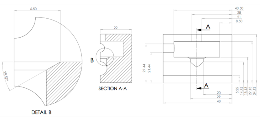
Figure 36: Frame dimension.

where $d^{*}$ is either $d_{{}_{max}}$ or either $d_{{}_{min}}$ and $\theta$ is the valve channel inclination as shown on Fig. 25. $\theta=29.53^{o}$ is obtained from Fig. 36 (DETAIL B). As expected, the final lift is always between these two limits.

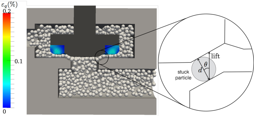
Figure 25: Final lift configuration; relation to stuck particle size.

Figure 27 (right) for $v_{p}=1\ m/s$ shows a lift of $\sim 0.00048\pm 0.00001\ m$ which is less than the minimum lift ($\text{lift}_{{}_{min}}=0.00155\pm 0.000001\ m$) for the smallest particle diameter in the polydispersity to travel through the valve. In fact here, as discussed previously in Section Quasi-steady open valve phase for the effect of $v_{p}$ on the lift, no particle flow is observed in the valve/rubber channel since the lift is less than one particle diameter. Therefore, when $v_{p}$ is turned off, the rubber descent is unimpeded by grains. Once the rubber makes contact with the valve seat, the fluid beneath the valve cannot escape and therefore a pressure and residual lift of $\sim 0.00048\pm 0.00001\ m$ remains, which is the lift when the rubber is in contact with the seat with zero deformation.

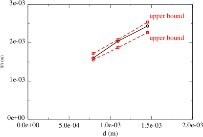
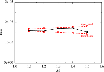
Figure 26: Final lift for different $d$ (left) and $\Delta d$ (right).

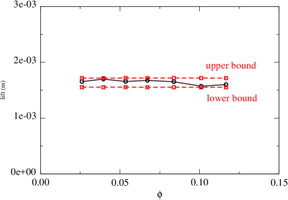
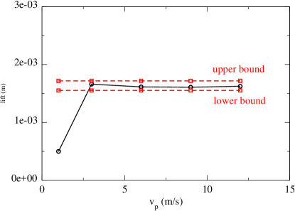
Figure 27: Final lift for different $\phi$ (left) and $v_{p}$ (right).

We give here a first quantitative view on which variables — among $d_{{}_{max}},\Delta d,\phi$ and $v_{p}$ — matter most in affecting the quantity of particles that get stuck beneath the valve during closure. Figure 28 and Fig. 29 show the projected area of particles on the seat (beneath valve-rubber area) normalized by the beneath valve-rubber area, i.e. the ‘normalized area of stuck particles’ (NASP). On these four figures, we find that $\phi$ matters most whereas there is little variation due to changes in $d_{{}_{max}}$, $v_{p}$ and $\Delta d$.

We can assume the packing fraction in the open valve channel, during the quasi-steady valve phase, is bounded below by $\phi$. As the valve descends during closure, particles are squeezed out and, as a further lower bound, we can approximate that a single monolayer at the same packing fraction $\phi$ remains. This implies the total number of stuck particles in the rubber-valve channel is approximated by: $N_{stuck}\simeq\text{lift}\ A\ \phi\ \frac{6}{\pi\ d^{3}}$ where the final lift is given by $\text{lift}\simeq d/\cos(\theta)$, and $A$ is the projected rubber-valve area. The projected total particle area is: $S_{stuck}\simeq\frac{d}{\cos(\theta)}\ A\ \phi\ \frac{6}{\pi\ d^{3}}\ \frac{\pi\ d^{2}}{4}\simeq\frac{3}{2}\frac{A}{\cos(\theta)}\ \phi$ normalizing the $S_{stuck}$ by $A$, we obtain:

$$\text{NASP}\simeq\frac{3}{2}\frac{1}{\cos(\theta)}\ \phi=1.72\phi$$ (34)

The above lower bound formula assumes that the final packing fraction of grains stuck in the valve is greater than the input value, $\phi$. In our tests we have observed that this is always true except for the one outlier case mentioned previously ($v_{p}=1\ m/s$, Fig. 20 (right)) where no particles travel through the channel because the beneath valve fluid pressure is less than the necessary pressure to open the valve to a lift greater than $d_{min}/\cos(\theta)$. This case is observed in Fig. 29 (left) ($v_{p}=1\ m/s$) where the normalized stuck area is zero.

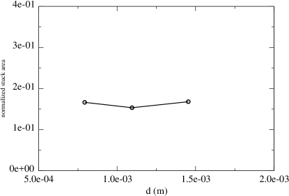
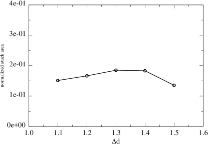
Figure 28: NASP for different $d$ (left) and $\Delta d$ (right).

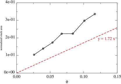
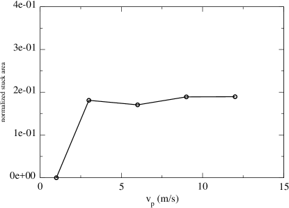
Figure 29: NASP for different $\phi$ (left) and $v_{p}$ (right).

If particles get stuck, they can also potentially break depending on the force of contact with the valve and seat, and grain properties such as the particle size and strength. A loose approximation of the possible volume of debris created can be made by assuming stuck particles all break. This may be expressed in terms of the final lift and the NASP, and then normalized by $d^{3}$, giving

$$\mbox{Debris}=\mbox{lift}\cdot A\cdot\text{NASP}/d^{3}$$ (35)

where $A$ is the valve-rubber projected area.

Supposing the lift obeys Eq. 33 where $d^{*}=d$ and NASP obeys Eq. 34, we suggest the Debris variable is approximated by:

$$\mbox{Debris}=\frac{3}{2}\frac{A}{\cos(\theta)^{2}}\frac{\phi}{d^{2}}$$ (36)

Figure 30 (left) shows the Debris as a function of $d$ and Fig. 30 (right) as a function of $\phi$. We show comparisons to our approximate formula (Eq. 36).

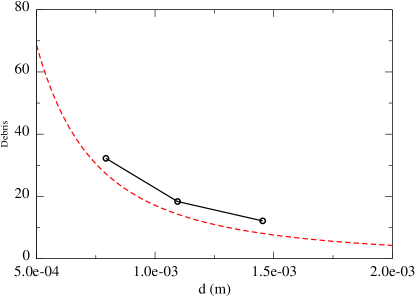
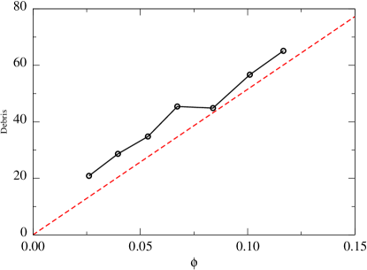
Figure 30: Debris variation as function $d$ (left) and $\phi$ (right). The red dashed line is the lower bound analytical solution (Eq. 36)

3.2 Safety valve lift behavior

Many of the behaviors in the safety valve configuration mimic those of the pressure valve. Here we summarize the safety valve data. The used input parameters are resumed in Tab. 3 for the simulations without particles and Tab. 4 for the simulations with particles.

Figure 31 shows the time evolution of the valve lift for different fluid viscosity (left) and for different piston velocity $v_{p}$; both simulations are without particles. The delay at the beginning of the simulation is less marked because of the absence of the above valve pressure. The steady lift shows many of the same behaviors as the pressure valve, except there can be non-zero $v_{p}$ (1 m/s and 2.5 m/s) and the valve may not ever open since the open end beneath the valve can prevent the beneath-valve pressure from building up enough to overcome the valve’s spring force to open it.

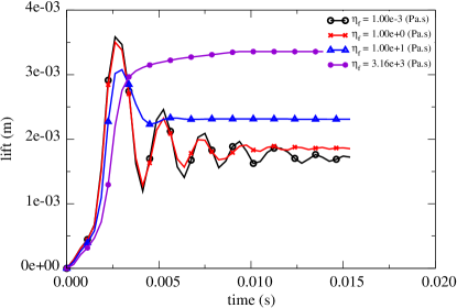
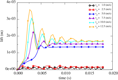
Figure 31: Valve lift as a function of time for different fluid viscosity (left) and different piston velocity (right) (without particles).

The three observed regimes for the pressure valve during the steady lift are also evidenced here as shown in Fig. 32 for different $\phi$ and $v_{p}$. The $\varphi_{{}_{l}}$ and $\varphi_{{}_{u}}$ need to be calculated here taking into account the outgoing flux through the modular closure of the safety valve system. This then becomes: $\varphi=\varphi_{{}_{in}}-\varphi_{{}_{out}}$ where $\varphi_{{}_{in}}$ is calculated from the input region and $\varphi_{{}_{out}}$ is calculated from the flux of outgoing particles through both outlet sections. Figure 33 (left) shows the time evolution of the valve lift for different $\Delta d$ where a small deviation in different values of $\Delta d$ is observed.

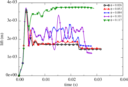
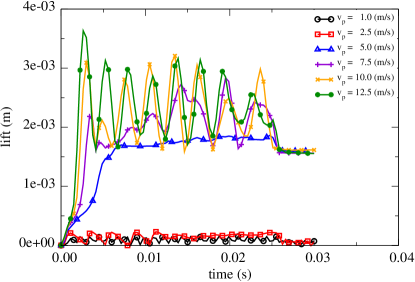
Figure 32: Valve lift as function of time for different packing fraction (left) and different piston velocity (right).

As shown in Fig. 25, the envelope of the final lift can be predicted by $\text{lift}=d^{*}/\cos(\theta)$, $d_{{}_{min}}\leqslant d^{*}\leqslant d_{{}_{max}}$ however, if the stuck particles are not entirely lodged in the valve channel, this prediction is wrong. This is the case in Fig. 33 (right) for $d=0.0014\ m$ where the final lift is less than the observed lift for $d=0.0011\ m$. Figure 34 shows that in fact no particles are fully stuck in the valve channel but there are some stuck in the rubber channel, as indicated by a non-zero normal force $\mbox{f}^{n}$. We see in Fig. 34 that even though contact exists between a partially stuck particle and the valve channel region, the total force coming from the valve channel is close to $\sim 0.1\ N$ whereas the total force observed in the rubber channel is close to $\sim 10\ N$; this means that the main force balancing the valve spring force comes from the rubber channel and therefore, the final lift is overpredicted by the previous formula, $\text{lift}=d^{*}/\cos(\theta)$.

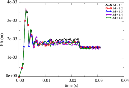
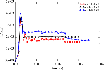
Figure 33: Valve lift as a function of time for different polydispercity (left) and different mean diameter (right).

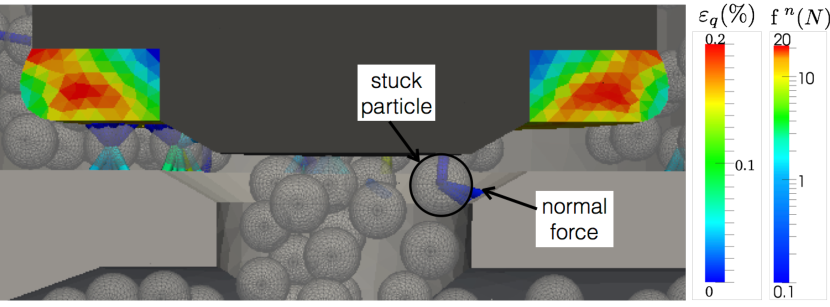
Figure 34: Final valve lift configuration for $d=0.0014\ m$ showing (partially) stuck particle in the valve entry and normal forces, $\mbox{f}^{\ n}$, supported by all particles.

The obtained results for both valves suggest that we may need more investigation with a broader range of particle input parameters to better make a comparison between the safety and the pressure valve geometries.

4 Conclusion

In this paper, we have presented a detailed implementation of a 3D DEM-LBM-Rubber coupling in two complex valve geometries. With different focused tests, we have validated the implemented methods. The coupling of the three types of materials shows a good agreement with our physical predictions. We also have demonstrated the validity of the ZIEB technique, which allowed us to run simulations without having to simulate the entire domain

Simulations performed without particles give realistic behaviors. We observe a lubrication effect causing suction that delays the opening of the valve after piston motion commences. We find that increasing fluid viscosity increasingly overdamps the valve lift, reducing or removing the valve oscillations in the quasi-steady regime. We have validated a Stokesian pressure drop across the valve channel when the fluid being driven through is sufficiently viscous.

In the simulations performed with particles in the pressure valve geometry, we found, for the steady lift portion, three qualitative lift behaviors. The different regimes appear to be governed by the total particle flux, which combines the imposed piston velocity $v_{p}$ and packing fraction $\phi$ through a flux $\varphi=v_{p}\ \phi$. The flux variable appears to indicate when the open-valve dynamics transition from a steady value of small lift, to an oscillating value that traverses between high and low positions, to a steady high lift value. Further investigation may be needed to calibrate the robustness of the $\varphi$ variable in determining qualitative valve dynamics.

The valve closure was also investigated, which occurs when the (virtual) piston motion is stopped. The pressure valve shows a dependency of the final lift on particle size and we give a prediction of the lift envelope based on the minimum and maximum particle sizes in the polydispersity. We show that if the maximum lift during the open phase does not exceed $d_{{}_{max}}/\cos(\theta)$, the final lift at closure can be less than $d_{{}_{min}}/\cos(\theta)$ because the particles are not entirely stuck in the valve channel.

Lastly we demonstrate the robustness of the approach by switching to a safety valve configuration, in which the above-valve region is not pressurized and the below-valve region has another exit. Similar qualitative behaviors are observed as compared to the pressure valve, both with and without particles, albeit at different specific values of the piston speed and input particle packing fraction.

Appendix A Safety valve, pressure valve, and their dimensions

In this appendix, we give the safety and pressure valve configuration and the dimensions. Units are millimeters $mm$ and degrees ^o.

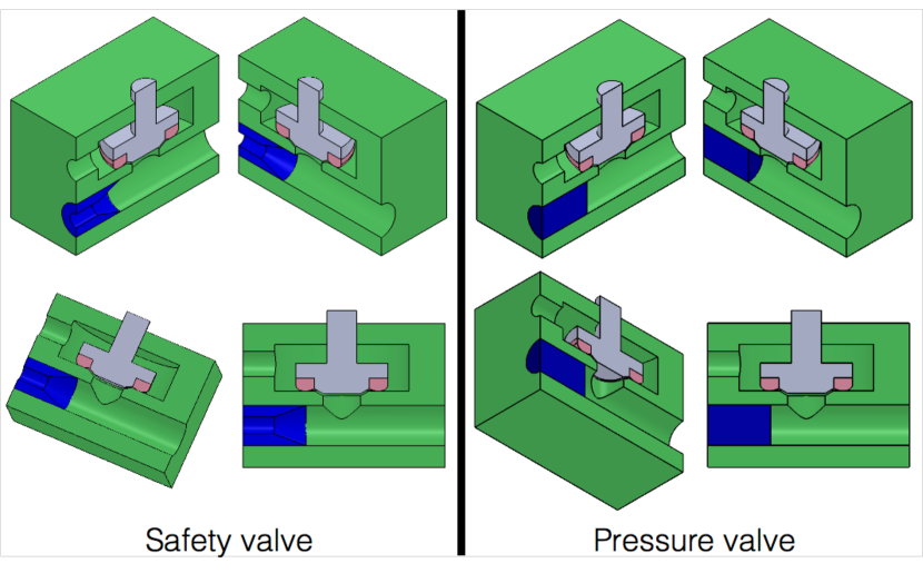
Figure 35: Safety and pressure valve configuration.

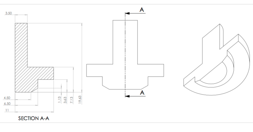
Figure 37: Valve dimension.

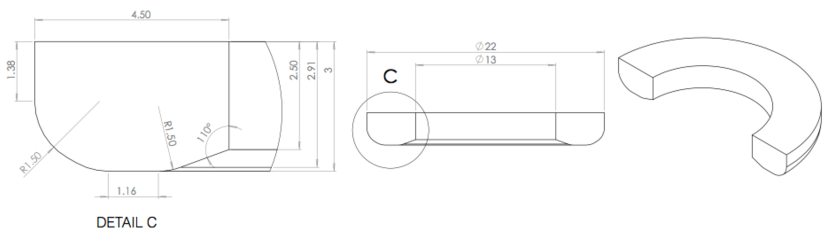
Figure 38: Rubber dimension.

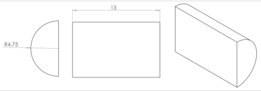
Figure 39: Pressure Closure dimension.

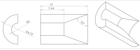
Figure 40: Safety Closure dimension.

References

- (1) M. Bouzidi, M. Firdaouss, P. Lallemand, Physics of Fluids 13, 3452 (2001)
- (2) Z. Guo, B. Shi, N. Wang, Journal of Computational Physics 165, 288 (2000)
- (3) Y.T. Feng, K. Han, D.R.J. Owen, International Journal For Numerical Methods In Engineering 72, 1111 (2007)
- (4) K. Han, Y.T. Feng, D.R.J. Owen, Computers & Structures 85, 1080 (2007)
- (5) K. Iglberger, N. Thürey, U. Rüde, Computers & Mathematics 55, 1461 (2008)
- (6) S. Hou, J. Sterling, S. Chen, G. Doolen, Pattern Formation and Lattice Gas Automata 6, 149 (1996)
- (7) C. Voivret, F. Radjaï, J.Y. Delenne, M.S. El Youssoufi, Physical Review E 76, 021301 (2007)
- (8) P.A. Cundall, The measurement and analysis of accelerations in rock slopes. Ph.D. thesis, Imperial College London (University of London) (1971)
- (9) M.P. Allen, D.J. Tildesley, Computer Simulation of Liquids (Oxford University Press, Oxford, 1987)
- (10) M. Jean, Computer Methods in Applied Mechanic and Engineering. 177, 235 (1999)
- (11) J.J. Moreau, in Powders & Grains 93 (A. A. Balkema, Rotterdam, 1993), p. 227
- (12) S. Luding, J. Duran, E. Clément, J. Rajchenbach, in Proc. of the 5th Chemical Engineering World Congress (AIChE, San Diego, 1996)
- (13) S. Luding, Granular Matter 10, 235 (2008)
- (14) F. Radjai, V. Richefeu, Mechanics of Materials 41, 715 (2009)
- (15) N.V. Brilliantov, T. Pöschel, Philos Transact A Math Phys Eng Sci 360, 415 (2002)
- (16) R. Hart, P. Cundall, J. Lemos, International Journal of Rock Mechanics and Mining Sciences & Geomechanics Abstracts. 25, 117 (1988)
- (17) W. O. R., Mechanics of Materials 16, 239 (1993)
- (18) Z.G. Feng, E.E. Michaelides, Journal of Computational Physics 195, 602 (2004)
- (19) Z. Yu, A. Wachs, Journal of Non-Newtonian Fluid Mechanics 145, 78 (2007)
- (20) X. He, L.S. Luo, Physical Review E 55, R6333 (1997)
- (21) S. Chapman, T. Cowling, The mathematical theory of nonuniform gases. (Cambridge University Press, 1970)
- (22) A. Satoh, Introduction to the practice of molecular simulation. (Elsevier Insights, 2011)
- (23) P. Bathnagar, E. Gross, M. Krook, Physical Review E 94, 511 (1954)
- (24) S. Chen, G. Doolen, Annual Review of Fluid Mechanics 30, 329 (1998)
- (25) X. He, L.S. Luo, J. Stat. Phys. 88, 927 (1997)
- (26) H. Yu, S.S. Girimaji, L.S. Luo, Journal of Computational Physics 209, 599 (2005)
- (27) R.H. Kraichnan, Journal of the Atmospheric Sciences 33, 1521 (1976)
- (28) J. Smaqorinsky, Mon. Wea. Rev., USWB 91, 99 (1963)
- (29) P. Moin, J. Kim, Journal of fluid mechanics 118, 341 (1982)
- (30) S. Hou, J. Sterling, S. Chen, G. Doolen, Pattern formation and lattice gas automata 6, 151 (1996)
- (31) D.Z. Yu, R.W. Mei, L.S. Luo, W. Shyy, Progress In Aerospace Sciences 39, 329 (2003)
- (32) L. Huabing, L. Xiaoyan, F. Haiping, Q. Yuehong, Physical review. E 70, 026701 (2004)
- (33) C. Peskin, Journal of Computational Physics 10(2), 252 (1972)
- (34) D. Wan, S. Turek, International Journal for Numerical Methods in Fluids 51, 531 (2006)
- (35) D. Wan, S. Turek, Journal of Computational and Applied Mathematics 203, 561 (2007)
- (36) R.V. A. J. C. Ladd, Journal of Statistical Physics 104(516) (2001)
- (37) P. Lallemand, L.S. Luo, Journal of Computational Physics 184, 1191 (2003)
- (38) M. Germano, U. Piomelli, P. Moin, W.H. Cabot, Physics of Fluids A: Fluid Dynamics 3(7), 1760 (1991)