Periodic orbits $1-5$ of quadratic polynomials on a new coordinate plane

Abstract.

While iterating the quadratic polynomial $f_{c}(x)=x^{2}+c$ the degree of the iterates grows very rapidly, and therefore solving the equations corresponding to periodic orbits becomes very difficult even for periodic orbits with a low period. In this work we present a new iteration model by introducing a change of variables into an $(u,v)$-plane, which changes situation drastically. As an excellent example of this we can compare equations of orbits period four on $(x,c)$- and $(u,v)$-planes. In the latter case, this equation is of degree two with respect to $u$ and it can be solved explicitly. In former case the corresponding equation $((((x^{2}+c)^{2}+c)^{2}+c)^{2}+c-x)/((x^{2}+c)^{2}+c-x)=0$ is of degree $12$ and it is thus much more difficult to solve.

1. Introduction

The dynamics of quadratic polynomials is often studied by using the family of maps $f_{c}(x)=x^{2}+c$, where $c\in\mathbb{C}$ (see, for example, [3], [6] and [10]). The orbit of the point $x_{0}\in\mathbb{C}$ is the sequence of points $x_{0},x_{1},x_{2},\ldots$, where $x_{n}=f_{c}(x_{n-1})=f_{c}^{n}(x_{0})$. In this work a central role is played by the periodic orbits or cycles of $f_{c}$ for which $f_{c}^{n}(x_{0})=x_{0}$ for some $n\in\mathbb{N}$. Now the number $n$ is the period of the orbit and $x_{0},x_{1},x_{2},\ldots x_{n-1}$ are periodic points of period $n$.

In this paper, we obtain the equations for the periodic orbits $1-5$ of the family $f_{c}$ by iterating the function

(1.1) $$G(u,v)=\left(\frac{-u+v+uv}{u},\frac{u^{2}-u+v-u^{2}v-uv+uv^{2}+v^{2}}{u}\right),$$

and forming the corresponding iterating system on the $(u,v)$-plane (in Section $2$). The function $G$ is a two-dimensional quadratic polynomial map which is defined in the complex 2-space $\mathbb{C}^{2}$ and its iteration reveals the dynamics of $f_{c}$. We will also compare the $(u,v)$-plane model to the $(x,y)$-plane model, which was introduced by Erkama in [5]. The purpose of developing this new model is that we obtain equations of periodic orbits of lower degree, which are easier to handle.

In the article [5] Erkama studied the dynamics of the polynomial family $f_{c}$ by iterating the function

$$F(x,y)=(y,y^{2}+y-x^{2})$$

on the $(x,y)$-plane, thus obtaining

$$P_{0}(x,y)=x_{0}=x,$$

$$P_{n+1}(x,y)=x_{n+1}=P_{n}(x,y)^{2}+y-x^{2}\qquad n=1,2,3,\ldots.$$

In this case $(x,y)$ is a periodic point of period $n$ so $F^{n}(x,y)=(x,y)$, if and only if $P_{n}(x,y)=x$. The set of periodic points is the union of all orbits whose period divides $n$. The formula $P_{n}=x_{n}$ was given by

(1.2) $$x_{n}=x_{1}+(x_{1}-x_{0})\sum_{\nu=1}^{n-1}(x_{0}+x_{n-1})(x_{0}+x_{n-2})\ldots(x_{0}+x_{n-\nu}),$$

where $n\geq 2$. Periodic orbits form algebraic curves corresponding to their periods. In this paper we present (in Sections $3-6$) the equations of these curves for periods $1-5$ on the $(u,v)$-plane. We also compare the figures of the real curves on the $(u,v)$-plane as well as on the $(x,y)$-plane. Figures and period equations of the $(x,y)$-plane for periods $1-4$ have appeared in [5], but period five in both cases and all models of the $(u,v)$-plane are previously unpublished. Moreover, we study the locations of neutral, attracting and repulsive fixed points on these curves ([1] and [2]) by using a suitable eigenvalue formula. By plotting attracting periodic points of the function $G$ we obtain a new version of the well-known period doubling bifurcation diagram (see, for example, [4], [7] and [9]) where the algebraic curves are of lower degree than previously (Figure 18). In the case of the function $F(x,y)$ we obtain Figure 17.

2. A new two-dimensional model for the quadratic family $f_{c}$ on the $(u,v)$-plane

It is well known that the dynamics of each quadratic polynomial is equivalent to the dynamics of $f_{c}$ for some $c\in\mathbb{C}$. In this section we form a new iteration model in which equations of periodic orbits are of remarkably lower of degree than in the earlier models. The new model is obtained from the $(x,y)$-plane model in [5] by the change of parameters

$$u = x+y$$

$$v = x+y^{2}+y-x^{2}.$$

Note that already this model obtained by Erkama on to the $(x,y)$-plane is of lower degree than other earlier models. Let’s check first some essential properties of the $(u,v)$-plane.

Theorem 2.1.

Singularities of the $(x,y)$-plane correspond to points $(u,v)=(0,0)$ and $u=(\infty,v)$, $v\in\mathbb{C}$ on the $(u,v)$-plane

Proof.

According to (1.2) we get

$$x_{0}+x_{2}=(x_{0}+x_{1})[1+(x_{1}-x_{0})]=(x_{0}+x_{1})[1+(x_{1}+x_{0})-2x_{0}].$$

Since $u=x_{0}+x_{1}$ and $v=x_{0}+x_{2}$, it follows by the previous formula that

$$v=u[1+u-2x_{0}]=u+u^{2}-2ux.$$

Figure 1. Curves $c=y-x^{2}$ on the $(x,y)$-plane with the parameter values $c=1/4$, $c=0$, $c=-1$, $c=-3/2$ and $c=-2$.

Figure 2. Curves $c=(-u^{4}+u^{2}(2v-3)-v^{2}+4uv)/(4u^{2})$ on the $(u,v)$-plane with the parameter values $c=1/4$, $c=0$, $c=-1$, $c=-3/2$ and $c=-2$.

Now $y=u-x$ so we can solve $x$ and $y$ in terms of variables $u$ and $v$ as follows

(2.1) $$x=\frac{u^{2}+u-v}{2u},\qquad y=\frac{u^{2}-u+v}{2u}.$$

We see easily that singularities of both of these expressions are $u=0$ and $u=\infty$. Furthermore, when $u=0$ it follows that also $v=0$. ∎

In the $(x,y)$-plane the mapping

(2.2) $$c:(x,y)\mapsto y-x^{2}$$

produces the parabola $f_{c}(x)=x^{2}+c$ depending on the point $c$ in the parameter space. In that case the orbits of periodic curves $P_{n}(x,y)=x$ are tangents to parabolas $y=f_{c}(x)$ at intersection points where period doubling occurs (see in [5], Figure $1$). The same way on the $(u,v)$-plane using formulas (2.1), the mapping

(2.3) $$c:(u,v)\mapsto\frac{-u^{4}+u^{2}(2v-3)-v^{2}+4uv}{4u^{2}}$$

produces a curve which corresponds to a point $c$ in the parameter space. Similarly on the $(u,v)$-plane the orbits of periodic curves are tangents to curves (2.3) at the bifurcation points. Curves $c(x,y)=y-x^{2}$ and $c(u,v)=(-u^{4}+u^{2}(2v-3)-v^{2}+4uv)/(4u^{2})$ are presented (Figure 1) and (Figure 2) with parameter values $c=1/4$, $c=0$, $c=-1$, $c=-3/2$ and $c=-2$.

It was obtained in [5] that the real Mandelbrot set of the function $F(x,y)$ when $c\in\mathbb{R}$ is

(2.4) $$\mathrm{M}_{\mathbb{R}}(F)=\{(x,y)|x=0,y\in[-2,1/4]\}.$$

On the line $x=0$ lie so called $\displaystyle{central\ critical\ points}$ of $F$ (see theorem (2.3)). This means that there is always one critical point on the curve at every critical cycle of every period. In what follows we check the Mandelbrot set on the $(u,v)$-plane when

$$u = x_{0}+x_{1}=x+y,$$

$$v = x_{0}+x_{2}=x+y^{2}+y-x^{2}=u(1+y-x).$$

Now the Mandelbrot set $\mathrm{M(G)}$ of the function $G(u,v)$ includes all points $c\in\mathbb{C}$ such that the sequence $\{G^{n}(c,c^{2}+c)\}$ is bounded. The sequence $\{G^{n}(c,c^{2}+c)\}$ is bounded in the space $\mathbb{C}^{2}$, if and only if the sequence $\{f_{c}^{n}(0)\}$ is bounded in the space $\mathbb{C}$.

Theorem 2.2.

The real Mandelbrot set of the function $G(u,v)$ is

$$\mathrm{M}_{\mathbb{R}}(G)=\{(u,v)|v=u^{2}+u,u\in[-2,1/4],v\in[-1/4,2]\}.$$

Proof.

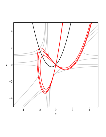
Figure 16. Curves of period $5$ orbits, critical curve $v=u^{2}+u$ and curves $c(u,v)=a$, when $a$ is $-1.62541372512376$, $-1.86078252220400$ and $-1.98542425305466$ on the $(u,v)$-plane.

If $x=0$ on the $(x,y)$-plane, it follows that $u=y$ on the $(u,v)$-plane. The first equation of (2.1) implies $v=u^{2}+u(1-2x)$ and thus we get $v=u^{2}+u=y^{2}+y$ on the line $x=0$. Now by (2.4) at the endpoints we have $v(-2)=2$ and $v(\frac{1}{4})=\frac{5}{16}$. When $v^{\prime}(u)=0$ the solution is $u=-\frac{1}{2}$ and further $v(-\frac{1}{2})=-\frac{1}{4}$. So the real Mandelbrot set on the $(u,v)$-plane is on the parabola $v=u^{2}+u$ (see Figure 16), which is also so called critical curve of the function $G$ like we see by the next result. ∎

This curve $v=u^{2}+u$ includes also all central critical points on $(u,v)$-plane. Let us define the universal filled Julia set $\mathrm{K(G)}$ as the set of all points $(u,v)\in\mathbb{C}^{2}$ such that the sequence $\{G^{n}(u,v)\}$ is bounded. Then the Mandelbrot set can also be described as the intersection of $K(G)$ with the parabola $v=u^{2}+u$.

Theorem 2.3.

The central critical points of $G(u,v)$ lie on the parabola $v=u^{2}+u$.

Proof.

The eigenvalue $\lambda_{n}(x,y)$ of $F^{n}(x,y)=(P_{n},P_{n}^{2}+y-x^{2})$ of periodic point $(x,y)$ of period $n$ is the Jacobian $det(J_{F})$ ([5])

(2.5) $$\lambda_{n}(x,y)=\frac{\partial P_{n}(x,y)}{\partial x}+2x\frac{\partial P_{n}(x,y)}{\partial y}.$$

For the critical points we have $\lambda_{n}(x,y)=0$, $n=1,2,3,\ldots$. When $P_{n}=P_{n-1}^{2}+y-x^{2}$ we obtain, based on the chain rule,

$$\lambda_{n}(x,y) = \frac{\partial P_{n}(x,y)}{\partial x}+2x\frac{\partial P_{n}(x,y)}{\partial y}$$

$$= 2P_{n-1}(x,y)\frac{\partial P_{n-1}(x,y)}{\partial x}\frac{\partial P_{n-2}(x,y)}{\partial x}\ldots\frac{\partial P_{1}(x,y)}{\partial x}-2x$$

$$+2x\left(2P_{n-1}(x,y)\frac{\partial P_{n-1}(x,y)}{\partial y}\frac{\partial P_{n-2}(x,y)}{\partial y}\ldots\frac{\partial P_{1}(x,y)}{\partial y}+1\right)$$

$$=2P_{n-1}(x,y)\left(\frac{\partial P_{n-1}(x,y)}{\partial x}\frac{\partial P_{n-2}(x,y)}{\partial x}\ldots\frac{\partial P_{1}(x,y)}{\partial x}\right)$$

$$+4xP_{n-1}(x,y)\left(\frac{\partial P_{n-1}(x,y)}{\partial y}\frac{\partial P_{n-2}(x,y)}{\partial y}\ldots\frac{\partial P_{1}(x,y)}{\partial y}\right).$$

Since $\partial P_{1}(x,y)/\partial x=0$ and $\partial P_{1}(x,y)/\partial y=1$, the critical points lie on the line $x=0$. Now by (2.1) we get $(u^{2}+u-v)/2u=0$, so $v=u^{2}+u$. ∎

In our new $(u,v)$-plane model we write

$$(u_{0},v_{0}) = (x_{0}+x_{1},x_{0}+x_{2})=(x+y,x+y^{2}+y-x^{2})$$

$$(u_{1},v_{1}) = (x_{1}+x_{2},x_{1}+x_{3})$$

$$= (y+y^{2}+y-x^{2},y+(y^{2}+y-x^{2})^{2}+y-x^{2}).$$

By using formulas (2.1) we get

$$u_{1}=\frac{-u+v+uv}{u}$$

and

$$v_{1}=\frac{u^{2}-u+v-u^{2}v-uv+uv^{2}+v^{2}}{u}.$$

Now the dynamics of the $(u,v)$-plane is determined be the iteration of the function $G$ defined by

$$G(u,v) = \left(\frac{-u+v+uv}{u},\frac{u^{2}-u+v-u^{2}v-uv+uv^{2}+v^{2}}{u}\right)$$

$$= (v+v/u-1,(v+v/u-1)(1+v-u))$$

$$= (g_{1},g_{1}(1+v-u)),$$

where

$$g_{1}=\frac{-u+v+uv}{u}.$$

Definition 2.4.

If

$$G(u,v) = (R(u,v),Q(u,v))$$

$$= \left(\frac{-u+v+uv}{u},\frac{u^{2}-u+v-u^{2}v-uv+uv^{2}+v^{2}}{u}\right),$$

then recursively

(2.6) $$\left\{\begin{array}[]{l}(R_{0}(u,v),Q_{0}(u,v))=(u,v),\\ \\ (R_{1}(u,v),Q_{1}(u,v))=(R(u,v),Q(u,v)),\\ \\ (R_{n+1}(u,v),Q_{n+1}(u,v))=G(R_{n}(u,v),Q_{n}(u,v)),\end{array}\right.$$

where

(2.7) $$\left\{\begin{array}[]{l}R_{n+1}(u,v)=Q_{n}(u,v)-1+Q_{n}(u,v)/R_{n}(u,v)\\ \\ Q_{n+1}(u,v)=R_{n+1}(u,v)(1+Q_{n}(u,v)-R_{n}(u,v)),\end{array}\right.$$

when $n=0,1,2,\ldots$.

Now $(u,v)$ is a periodic point of period $n$, so $G^{n}(u,v)=(u,v)$, if and only if $(R_{n}(u,v),Q_{n}(u,v))$=$(u,v)$. The set of periodic points is the union of all orbits, whose period divides $n$.

Due to the form of the definition of an eigenvalue on the $(u,v)$-plane, it is convenient to denote $T_{n+1}(u,v)=1+Q_{n}(u,v)-R_{n}(u,v)$, and write the formula $(\ref{6})$ in the form

$$\left\{\begin{array}[]{l}R_{n+1}(u,v)=Q_{n}(u,v)-1+Q_{n}(u,v)/R_{n}(u,v)\\ \\ Q_{n+1}(u,v)=R_{n+1}(u,v)(1+Q_{n}(u,v)-R_{n}(u,v))=R_{n+1}(u,v)T_{n+1}(u,v).\end{array}\right.$$

Now the Jacobian of the function $G^{n}(u,v)=G(R_{n-1}(u,v),Q_{n-1}(u,v))$
$=(R_{n}(u,v),Q_{n}(u,v))=(R_{n}(u,v),R_{n}(u,v)T_{n}(u,v))$ is of the form

$$\begin{array}[]{ll}\displaystyle{\det}(J_{G})&=\displaystyle{\det}\displaystyle{\begin{pmatrix}\displaystyle\frac{\partial R_{n}}{\partial u}&\displaystyle\frac{\partial R_{n}}{\partial v}\\ \displaystyle\frac{\partial Q_{n}}{\partial u}&\displaystyle\frac{\partial Q_{n}}{\partial v}\end{pmatrix}}=\displaystyle{\det}\displaystyle{\begin{pmatrix}\displaystyle\frac{\partial R_{n}}{\partial u}&\displaystyle\frac{\partial R_{n}}{\partial v}\\ \displaystyle\frac{\partial R_{n}}{\partial u}T_{n}+R_{n}\frac{\partial T_{n}}{\partial u}&\displaystyle\frac{\partial R_{n}}{\partial v}T_{n}+R_{n}\frac{\partial T_{n}}{\partial v}\end{pmatrix}}\\ \\ &=\displaystyle{R_{n}\Big{(}\frac{\partial R_{n}}{\partial u}\frac{\partial T_{n}}{\partial v}-\frac{\partial R_{n}}{\partial v}\frac{\partial T_{n}}{\partial u}\Big{)}}.\end{array}$$

For the periodic points $(u,v)$ of period $n$ we have $R_{n}(u,v)=u$. Because of this, the eigenvalue $\lambda_{n}(u,v)$ of a periodic point of period $n$ of the function $G^{n}(u,v)$ is of the form

(2.8) $$\lambda_{n}(u,v)=u\Big{(}\frac{\partial R_{n}}{\partial u}\frac{\partial T_{n}}{\partial v}-\frac{\partial R_{n}}{\partial v}\frac{\partial T_{n}}{\partial u}\Big{)},$$

when $n=1,2,\ldots$.

On the $(u,v)$-plane fixed points and periodic points are classified in the following way:

Definition 2.5.

Let us assume that $(u,v)\in\mathbb{C}^{2}$ is a periodic point of period $n$ of the function $G(u,v)$. In that case $(u,v)$ is

$$1. \textrm{attracting},\ \textrm{if}\ 0<|\lambda_{n}(u,v)|<1,$$

$$2. \textrm{super-attracting or critical},\ \textrm{if}\ \lambda_{n}(u,v)=0,$$

$$3. \textrm{repulsive},\ \textrm{if}\ |\lambda_{n}(u,v)|>1,$$

$$4. \textrm{indifferent (neutral)},\ \textrm{if}\ |\lambda_{n}(u,v)|=1,$$

when $n=1,2,3,\ldots$.

3. Periodic orbits of periods $1-2$

In this section we obtain periodic orbit equations of period one and two, and classify these points based on definition 2.5 on the $(u,v)$-plane.

Fixed points of period one on the $(u,v)$-plane satisfy a pair of equations
$G(R_{0}(u,v),Q_{0}(u,v))=(u,v)$, where

(3.1) $$\left\{\begin{array}[]{l}R_{1}(u,v)=(-u+v+uv)/u=u\\ Q_{1}(u,v)=(-u^{2}+u-v+u^{2}v+uv-uv^{2}-v^{2})/u=v.\end{array}\right.$$

The first equation is equivalent with

$$u^{2}+u-v-uv=(u-v)(1+u)=0.$$

When $u=-1$, the second equation is not satisfied so $v=u$ is the only solution for both of them. Thus $v=u$ is the equation of period one orbits. We obtain neutral periodic points of period one when $v=u$, and by (2.8) the eigenvalue is

$$|\lambda_{1}(u,v)|=\left|\frac{{u}^{2}+u-v}{u}\right|=1,$$

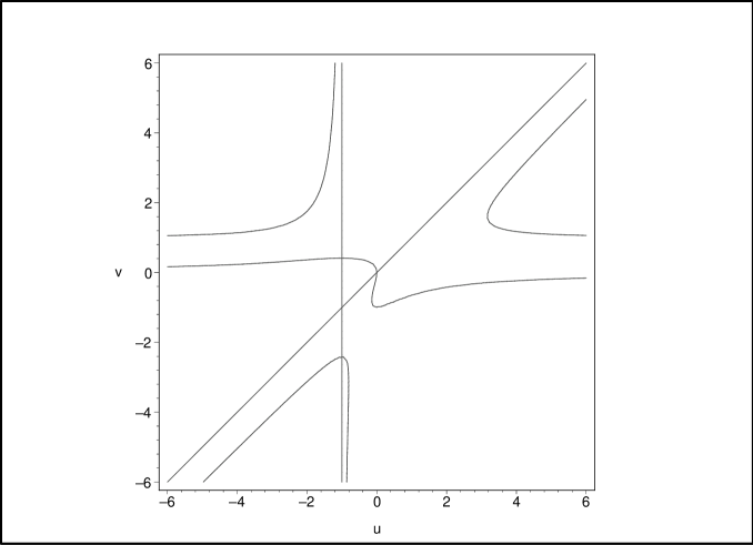
Figure 6. Curves of period $1$, $2$ and $4$ orbits on the $(u,v)$-plane.

and thus these are $(u,v)=(-1,-1)$ and $(u,v)=(1,1)$ (corresponding on the $(x,y)$-plane to $(x,y)=(-1/2,-1/2)$ and $(x,y)=(1/2,1/2)$). Thus the only real bifurcation point is $(u,v)=(-1,-1)$ (corresponding on the $(x,y)$-plane to $(x,y)=(-1/2,-1/2)$), which we obtained as the intersection of period one and two orbits (Figures 5 and 6). The origin is the only critical point (or super-attracting point) and it is located on the parabola $v=u^{2}+u$. Because of that the line segment

$$\{(u,v)|v=u,u\in[-1,1],v\in[-1,1]\}$$

is located in the Fatou set. We see this clearly in the bifurcation diagram (Figure 18). Similarly the origin is the only critical point on the $(x,y)$-plane. Naturally the complement

$$V_{1}(u,v)\setminus\{(u,v)|v=u,u\in[-1,1],v\in[-1,1]\},$$

where $V_{1}(u,v)$ is an affine variety of period one, is located in the Julia set.

As for periodic points of period two, they satisfy the pair of equations $G^{2}=(u,v)$, or

(3.2) $$\left\{\begin{array}[]{ll}R_{2}(u,v)=&(-u+v-u^{2}v+uv^{2}+v^{2})/u=u\\ Q_{2}(u,v)=&(-u^{2}+uv+3u^{2}v-2uv^{2}-u^{3}+v^{4}+v^{3}+u^{4}v^{2}-u^{4}v)/u^{2}\\ &+(3u^{3}v^{2}-2u^{3}v^{3}-4u^{2}v^{3}-uv^{3}+u^{2}v^{4}+2uv^{4})/u^{2}=v.\end{array}\right.$$

The first equation can be written in the form

$$-(v+1)(u+1)(u-v)=0.$$

and therefore $u=-1$ is the equation of period two orbits, because it is the only one satisfied by the pair of equations (3.2).

We obtain neutral periodic orbits of period two when $u=-1$ in the formula $|\lambda_{2}(u,v)|=1$. Now

$$|\lambda_{2}(u,v)|=\left|\frac{\left({u}^{2}+u-v\right)\left({u}^{2}-u+v\right)}{{u}^{2}}\right|=1,$$

and this is equivalent with the pair of equations

$$\left\{\begin{array}[]{l}-v^{2}-2v-1=0\\ -v^{2}-2v+1=0,\end{array}\right.$$

when $u=-1$. The solutions of the eigenvalue equation $|\lambda_{2}(-1,v)|=1$ are $(u,v)=(-1,-1+\sqrt{2})$, $(u,v)=(-1,-1-\sqrt{2})$ and $(u,v)=(-1,-1)$, which is a double root. The real neutral cycles of period two are thus $(-1,-1+\sqrt{2}),(-1,-1)$ and $(-1,-1-\sqrt{2}),(-1,-1)$ and these include also a neutral fixed point of period one. The bifurcation points of period two are also real neutral periodic points of period two and they are $(u,v)=(-1,-1+\sqrt{2})$ and $(u,v)=(-1,-1-\sqrt{2})$ on the $(u,v)$-plane (Figure 6), as well as $(x,y)=(\frac{-1-\sqrt{2}}{2},\frac{-1+\sqrt{2}}{2})$ and $(x,y)=(\frac{-1+\sqrt{2}}{2},\frac{-1-\sqrt{2}}{2})$ on the $(x,y)$-plane (Figure 5). Bifurcation points of period two are obtained also as intersection points of period four orbit, because the curve of period two bifurcates to curves of period four. We obtain all critical points of period two when the eigenvalue equation $|\lambda_{2}(u,v)|=0$ holds. In that case ${u}^{2}+u-v=0$ or ${u}^{2}-u+v=0$. When $u=-1$ we obtain cycles of critical points of period two on the $(u,v)$-plane as $(u,v)=(-1,0)$ and $(u,v)=(-1,-2)$ as well as on the $(x,y)$-plane as $(x,y)=(0,-1)$ and $(x,y)=(-1,0)$. Because $(u,v)=(-1,-1/2)$ is an attracting fixed point ($|\lambda_{2}(-1,-1/2)|<1$), then

$$V_{2}(u,v)\setminus\left(\{(u,v)|u=-1,v\in[-1-\sqrt{2},-1+\sqrt{2}]\}\right)=V_{2}(u,v)\setminus F(G)$$

belongs to the Julia set.

When we solve the pair of equations (2.7) to higher periods, the situation gets complicated very fast due to the growth of degree in the equations. The following result is very useful in sections $4-6$.

Theorem 3.1.

The pair of equations

(3.3) $$\left\{\begin{array}[]{ll}R_{0}R_{1}R_{2}\cdots R_{n}=&1\\ Q_{0}Q_{1}Q_{2}\cdots Q_{n}=&1,\end{array}\right.$$

where $n=0,1,2,\ldots$, satisfies the equation of period $n+1$ orbits.

Proof.

Let us define $P_{k+1}=x_{k}^{2}+c$ and $P_{l+1}=x_{l}^{2}+c$, when $k,l\in\mathbb{N}$. Now we notice that $P_{k+1}-P_{l+1}=x_{k}^{2}-x_{l}^{2}=(x_{k}-x_{l})(x_{k}+x_{l})$, and so

(3.4) $$x_{k}+x_{l}=\frac{P_{k+1}-P_{l+1}}{x_{k}-x_{l}}=\frac{x_{k+1}-x_{l+1}}{x_{k}-x_{l}}$$

for all $k,l\in\mathbb{N}$. Because $R_{0}=u=x_{0}+x_{1}$ and $Q_{0}=v=x_{0}+x_{2}$, we get the next product by using (3.4), as follows:

$$R_{0}R_{1}R_{2}\cdots R_{n} = (x_{0}+x_{1})(x_{1}+x_{2})(x_{2}+x_{3})\cdots(x_{n}+x_{n+1})$$

$$= \Big{(}\frac{x_{1}-x_{2}}{x_{0}-x_{1}}\Big{)}\Big{(}\frac{x_{2}-x_{3}}{x_{1}-x_{2}}\Big{)}\Big{(}\frac{x_{3}-x_{4}}{x_{2}-x_{3}}\Big{)}\cdots\Big{(}\frac{x_{n+1}-x_{n+2}}{x_{n}-x_{n+1}}\Big{)}$$

$$= \frac{x_{n+1}-x_{n+2}}{x_{0}-x_{1}}.$$

Let us assume that $x_{n+1}=P_{n+1}=x_{0}=x$. Then $x_{n+2}=P_{n+2}=x_{n+1}^{2}+c=x_{0}^{2}+c=x_{1}$, so

$$R_{0}R_{1}R_{2}\cdots R_{n}=\frac{x_{n+1}-x_{n+2}}{x_{0}-x_{1}}=\frac{x_{0}-x_{1}}{x_{0}-x_{1}}=1$$

and the assertion follows. Similarly

$$Q_{0}Q_{1}Q_{2}\cdots Q_{n} = (x_{0}+x_{2})(x_{1}+x_{3})(x_{2}+x_{4})\cdots(x_{n}+x_{n+2})$$

$$= \Big{(}\frac{x_{1}-x_{3}}{x_{0}-x_{2}}\Big{)}\Big{(}\frac{x_{2}-x_{4}}{x_{1}-x_{3}}\Big{)}\Big{(}\frac{x_{3}-x_{5}}{x_{2}-x_{4}}\Big{)}\cdots\Big{(}\frac{x_{n+1}-x_{n+3}}{x_{n}-x_{n+2}}\Big{)}$$

$$= \frac{x_{n+1}-x_{n+3}}{x_{0}-x_{2}}=1,$$

when $x_{n+3}=x_{n+2}^{2}+c=(x_{n+1}^{2}+c)^{2}+c=(x_{0}^{2}+c)^{2}+c=x_{1}^{2}+c=x_{2}$. ∎

4. Periodic orbits of period $3$

Fixed points of period three satisfy the pair of equations

(4.1) $$\left\{\begin{array}[]{ll}R_{3}(u,v)=&(-{u}^{2}+uv+{u}^{2}v-{u}^{3}v+{u}^{2}{v}^{2}-u{v}^{2}+{v}^{4}+{v}^{3}\\ &+{u}^{4}{v}^{2}-{u}^{4}v+3\,{u}^{3}{v}^{2}-2\,{u}^{3}{v}^{3}-4\,{u}^{2}{v}^{3}-u{v}^{3}\\ &+{u}^{2}{v}^{4}+2\,u{v}^{4})/{u}^{2}=u\\ \\ Q_{3}(u,v)=&(-8\,{u}^{3}{v}^{3}+5\,{u}^{3}{v}^{2}-3\,{u}^{4}v+7\,{u}^{4}{v}^{2}+{u}^{3}v+6\,{u}^{2}{v}^{4}\\ &-3\,{u}^{2}{v}^{3}+u{v}^{4}-{u}^{4}+{u}^{6}v-{u}^{7}{v}^{2}+{u}^{7}v+{u}^{8}{v}^{4}\\ &+{u}^{8}{v}^{2}+{u}^{4}{v}^{8}+6\,{u}^{6}{v}^{3}-3\,{u}^{5}v-8\,{u}^{6}{v}^{2}-4\,{u}^{5}{v}^{2}\\ &+23\,{u}^{5}{v}^{3}+8\,{u}^{4}{v}^{3}-35\,{u}^{4}{v}^{4}-11\,{u}^{3}{v}^{4}-3\,u{v}^{5}+31\,{u}^{3}{v}^{5}\\ &+10\,{u}^{2}{v}^{5}-11\,{u}^{5}{v}^{4}+6\,{u}^{4}{v}^{5}-6\,u{v}^{6}+6\,{u}^{3}{v}^{6}-15\,{u}^{2}{v}^{6}\\ &+34\,{v}^{6}{u}^{4}-22\,{v}^{7}{u}^{3}-10\,{v}^{7}{u}^{2}+2\,{v}^{7}u+6\,{v}^{8}{u}^{2}+4\,{v}^{8}u\\ &-2\,{u}^{8}{v}^{3}+10\,{u}^{7}{v}^{4}-4\,{u}^{7}{v}^{5}-22\,{u}^{6}{v}^{5}-30\,{u}^{5}{v}^{5}\\ &+6\,{u}^{6}{v}^{6}+26\,{u}^{5}{v}^{6}-6\,{u}^{7}{v}^{3}+17\,{u}^{6}{v}^{4}-4\,{u}^{5}{v}^{7}\\ &-16\,{u}^{4}{v}^{7}+4\,{u}^{3}{v}^{8}+{u}^{5}+{v}^{8}+2\,{v}^{7}+{v}^{6})/{u}^{4}=v.\end{array}\right.$$

On the other hand, we know that (3.3) is satisfied for period three orbits, when

(4.2) $$1=R_{0}R_{1}R_{2}.$$

Using formulas (3.1) and (3.2), it follows that the previous equation (4.2) takes the form, which can be factorized as

$$-{\frac{\left(uv+1+v\right)\left(-{u}^{2}+{u}^{2}v-u{v}^{2}+uv+u-{v}^{2}\right)}{u}}=0,$$

where both of polynomials are undivisible. This equation is satisfied when

$$uv+1+v=0,$$

or

$$-{u}^{2}+{u}^{2}v-u{v}^{2}+uv+u-{v}^{2}={u}^{2}(v-1)+u(1+v-{v}^{2})-{v}^{2}=0.$$

Solutions of the latter equation are

$$u=\frac{1+v-{v}^{2}\pm\sqrt{{v}^{4}+2\,{v}^{3}-5\,{v}^{2}+2\,v+1}}{2v-2},$$

which does not satisfy system of equations (4.1). Instead, the solution

(4.3) $$v=-\frac{1}{1+u},$$

is the equation for the period three orbits. Moreover we notice that the pair of equations

$$\left\{\begin{array}[]{l}uv+1+v=0\\ {u}^{2}(v-1)+u(1+v-{v}^{2})-{v}^{2}=0\end{array}\right.$$

and the equation

$$\frac{-u^{4}-2u^{3}-u^{2}-u-1}{(u+1)^{2}}=\frac{-{u}^{3}-{u}^{2}-1}{u+1}=0$$

are equivalent. Both of them have only one real solution. By a numerical approximation we obtain solutions

$$\begin{array}[]{l}(u,v)=(-1.465571232,2.147899035),\\ (u,v)=(.2327856159-.7925519930i,-.5739495176-.3689894075i),\\ (u,v)=(.2327856159+.7925519930i,-.5739495176+.3689894075i).\end{array}$$

The equation (4.3) for period three is of degree three on the $(x,y)$-plane for both variables and its solutions are

$$j_{1}=\big{(}A+\sqrt{B}\big{)}^{1/3}+\big{(}A-\sqrt{B}\big{)}^{1/3}-\frac{2}{3}-\frac{1}{3}x,$$

$$j_{2}=C\big{(}A+\sqrt{B}\big{)}^{1/3}+C^{2}\big{(}A-\sqrt{B}\big{)}^{1/3}-\frac{2}{3}-\frac{1}{3}x$$

and

$$j_{3}=C^{2}\big{(}A+\sqrt{B}\big{)}^{1/3}+C\big{(}A-\sqrt{B}\big{)}^{1/3}-\frac{2}{3}-\frac{1}{3}x,$$

where

$$A={\frac{8}{27}}\,{x}^{3}-\frac{2}{9}{x}^{2}-\frac{1}{9}x-{\frac{25}{54}},$$

$$B={\frac{4}{27}}\,{x}^{4}+{\frac{4}{27}}\,{x}^{3}-{\frac{5}{27}}\,{x}^{2}-\frac{1}{9}\,x-{\frac{23}{108}}$$

and

$$C=-\frac{1}{2}+\frac{\sqrt{3}}{2}i$$

by Cardano’s formulas. There is a remarkable difference compared to the equation (4.3), which is only degree one on the $(u,v)$-plane.

The eigenvalue of period three in the $(u,v)$-plane is

$$\lambda_{3}(u,v)=-{\frac{\left(-{u}^{2}-u+v\right)\left({u}^{2}-u+v\right)\left(-{u}^{2}-u+v+2\,uv\right)}{{u}^{3}}}.$$

Now we get neutral periodic points by solving the pair of equations

(4.4) $$\left\{\begin{array}[]{l}1+v+vu=0\\ |\left({u}^{2}+u-v\right)\left({u}^{2}-u+v\right)\left(-{u}^{2}-u+v+2\,uv\right)/{u}^{3}|=1.\end{array}\right.$$

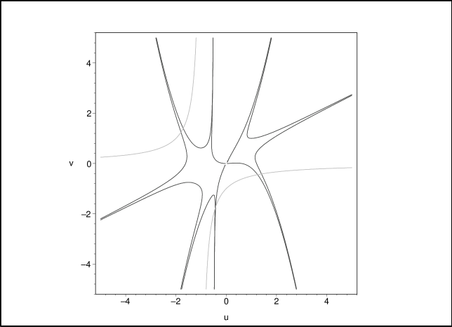
Figure 4. Curves of period three orbits and eigenvalues $|\lambda_{3}(u,v)|=1$.

Also in the case of period three, neutral fixed points are bifurcation points. The system of equations (4.4) produces neutral fixed points and also all cycles of bifurcation points of period three. All bifurcation points of period three (there are $18$ but the points $(u,v)=(-1/2+i\sqrt{3}/2,-1/2+i\sqrt{3}/2)$ and $(u,v)=(-1/2-i\sqrt{3}/2,-1/2-i\sqrt{3}/2)$ are roots of order three) are shown in Table $3.1$. Out of them six are real (two cycles of three points) and eight are complex points. We see the real points in Figure 4. Also we see what parts of period three curves belong to the Julia and the Fatou sets. Attracting periodic points form well known windows of period three in the bifurcation diagram, which we see clearly in the lowest part in pictures both on the $(u,v)$-plane (Figure 18) and the $(x,y)$-plane (Figure 17).

Table $3.1$.

Bifurcation points of period three on the $(u,v)$-plane.

$$\begin{array}[]{|ll|}\hline\cr u=-1.71331833&v=1.401899029\\ \hline\cr u=-1.801937736&v=1.246979604\\ \hline\cr u=1.246979604&v=-.4450418679\\ \hline\cr u=1.401899029&v=-.4163372349\\ \hline\cr u=-.41633724&v=-1.713318135\\ \hline\cr u=-.4450418660&v=-1.801937733\\ \hline\cr u=-.8952981106+1.448231193i&v=-.04966091024+.6869071824i\\ \hline\cr u=-.691162865+.49957401i&v=-.8952981114+1.448231194i\\ \hline\cr u=-.049660912+.686907179i&v=-.6911628079+.4995739964i\\ \hline\cr u=-.049660912-.686907179i&v=-.6911628079-.4995739964i\\ \hline\cr u=-.691162865-.49957401i&v=-.8952981114-1.448231194i\\ \hline\cr u=-.8952981106-1.448231193i&v=-.04966091024-.6869071824i\\ \hline\cr u=-1/2+i\sqrt{3}/2&v=-1/2+i\sqrt{3}/2\\ \hline\cr u=-1/2-i\sqrt{3}/2&v=-1/2-i\sqrt{3}/2\\ \hline\cr\end{array}$$

We obtain all critical points or super-attractive points (Table $3.2$) as solutions of the pair of equations

(4.5) $$\left\{\begin{array}[]{l}1+v+vu=0\\ \left({u}^{2}+u-v\right)\left({u}^{2}-u+v\right)\left(-{u}^{2}-u+v+2\,uv\right)=0.\end{array}\right.$$

But then according to theorem 2.3 the central critical points of the $(u,v)$-plane lie on the curve $v=u^{2}+u$. Thus we obtain one point at each critical cycle of period three as a solution of the pair of equations

(4.6) $$\left\{\begin{array}[]{l}1+v+vu=0\\ v=u^{2}+u.\end{array}\right.$$

A great benefit of this method is that the system of equations is of significantly lower degree than system (4.5). The pair of equations (4.6) is equivalent with the equation

$$u^{3}+2u^{2}+u+1,$$

and a numerical approximation of its solutions are

$$\begin{array}[]{l}(u,v)=(-1.754877666,1.324717957),\\ (u,v)=(-.1225611669-.7448617670i,-.6623589783-.5622795121i),\\ (u,v)=(-.1225611669+.7448617670i,-.6623589783+.5622795121i).\end{array}$$

The rest of the points of the cycles are naturally obtained by iteration of the function $G$.

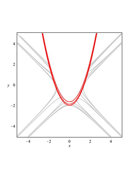
Figure 15. Curves of period $5$ orbits and curves $c(x,y)=a$, when $a$ is $-1.62541372512376$, $-1.86078252220400$ and $-1.98542425305466$ on the $(x,y)$-plane.

Further, we can also obtain all critical points of period three by calculating intersection points of tangent curves using, for example, the article of Stephenson and Ridgway [11]. In their article Stephenson and Ridgway have listed points of different periods on the line $x=0$ (central critical points $(0,c)$ on the $(x,y)$-plane). These points correspond to the bottom points of parabolas (2.2) (in the Mandelbrot set), which are tangential with the periodic points curves of the same period. Similarly, on the $(u,v)$-plane, critical points are obtained by formulating the corresponding equation (2.3) at this point $c$ and finding the pair of solutions $(u,v)$ of this equation (2.3) and equation of period three orbits (4.3). Corresponding curves on the $(u,v)$-plane are unlike on the $(x,y)$-plane, like we see in the Figure 2. In the period five case this property is shown in Figures 15 and 16.

Table $3.2$.

Critical points of period three orbits on the $(u,v)$-plane.

$$\begin{array}[]{|ll|}\hline\cr u=-1.754877667&v=1.324717959\\ \hline\cr u=1.324717957&v=-.4301597090\\ \hline\cr u=-.4301597100&v=-1.754877668\\ \hline\cr u=-.6623589786-.5622795121i&v=-.7849201455-1.307141279i\\ \hline\cr u=-.7849201452-1.307141279i&v=-.1225611670-.7448617664i\\ \hline\cr u=-.7849201455+1.307141279i&v=-.1225611669+.7448617666i\\ \hline\cr u=-.6623589786+.5622795121i&v=-.7849201455+1.307141279i\\ \hline\cr u=-.1225611669+.7448617670i&v=-.6623589792+.5622795123i\\ \hline\cr u=-.1225611669-.7448617670i&v=-.6623589792-.5622795123i\\ \hline\cr\end{array}$$

5. Periodic orbits of period $4$

Fixed points of period four satisfy the pair of equations

(5.1) $$\left\{\begin{array}[]{ll}R_{4}(u,v)=&u\\ Q_{4}(u,v)=&v.\end{array}\right.$$

In addition, we know that (3.3) is satisfied by period four orbits, when

(5.2) $$1=uR_{1}R_{2}R_{3}.$$

When we substitute these formulas of $R_{1}$, $R_{2}$ and $R_{3}$ into (5.2) and factorize, we get

(5.3) $$\frac{abc}{{u}^{3}}=0,$$

where

$$\begin{array}[]{ll}a=&-(1+u),\\ b=&-{u}^{2}v+{u}^{2}{v}^{2}-u+uv+u{v}^{2}-{v}^{2}-{v}^{3}-u{v}^{3},\\ c=&-{u}^{4}v+{u}^{4}{v}^{2}-2\,{u}^{3}{v}^{3}+3\,{u}^{3}{v}^{2}+{u}^{2}{v}^{4}-4\,{u}^{2}{v}^{3}+2\,{u}^{2}v-{u}^{2}+2\,u{v}^{4}-u{v}^{3}\\ &-2\,u{v}^{2}+{v}^{4}+{v}^{3}.\end{array}$$

This formula includes orbits of period two. Equation (5.3) is also satisfied when $b=0$ or $c=0$. Due to the intersection of curves of period four and two at the bifurcation points, period four orbits must be satisfied by $u=-1$. By substituting this to the equation $b=0$ we get

$$-v^{2}-2v+1=0,$$

the solutions of which are the bifurcation points $v=-1\pm\sqrt{2}$. Further if we substitute $u=-1$ to the equation $c=0$ we obtain $v-1=0$. This is the asymptotic line for the period four curve. In conclusion, the equation of period four curves is

$$-{u}^{2}v+{u}^{2}{v}^{2}-u+uv+u{v}^{2}-{v}^{2}-{v}^{3}-u{v}^{3}=0,$$

which can be written as

(5.4) $$u^{2}(-v^{2}+v)+u(v^{3}-v^{2}-v+1)+v^{3}+v^{2}=0$$

and solved explicitly as for factor $u$:

$$u=\frac{v^{3}-v^{2}-v+1\pm\sqrt{v^{6}+2v^{5}-v^{4}-v^{2}-2v+1}}{2(v^{2}-v)}.$$

On the $(x,y)$-plane the degree of the equation of period four orbits is six for both factors, thus it is impossible to solve them explicitly. The equation of period four orbits has been presented in the literature before now explicitly only twice; T. Erkama [5] presented nearly the same form at $2006$ and also Morton [8] presented a corresponding solution, but in a more complicated form at $1998$. Morton’s solution of period four orbits equation by using model $P(x)=x^{2}+c$ is

$$x=\frac{w}{2}\pm\frac{\triangle}{2(w^{3}-w)},$$

where

$$\triangle^{2}=(w^{4}-1)(w^{2}+2w-1),$$

and

$$w=x^{4}+2cx^{2}+x+c+c^{2}.$$

The eigenvalue of period four on the $(u,v)$-plane is

$$\lambda_{4}(u,v)=-{\frac{a_{4}b_{4}c_{4}d_{4}}{{u}^{4}}},$$

where

$$a_{4} = {u}^{2}+u-v,$$

$$b_{4} = {u}^{2}-u+v,$$

$$c_{4} = 2\,uv+v-u-{u}^{2},$$

$$d_{4} = 2\,u{v}^{2}+2\,{v}^{2}+v-2\,uv-u-2\,{u}^{2}v+{u}^{2}.$$

We obtain bifurcation points of period four as solutions of system of equations

$$\left\{\begin{array}[]{l}u^{2}(-v^{2}+v)+u(v^{3}-v^{2}-v+1)+v^{3}+v^{2}=0\\ |\lambda_{4}(u,v)|=1,\end{array}\right.$$

which have $56$ solutions all together. Real bifurcation points can be seen in Figure 8, where they are the intersection points of curves of period four and eigenvalues $|\lambda_{4}(u,v)|=1$. The central critical points are obtained as solutions of the pair of equations

$$\left\{\begin{array}[]{l}u^{2}(-v^{2}+v)+u(v^{3}-v^{2}-v+1)+v^{3}+v^{2}=0\\ v=u^{2}+u,\end{array}\right.$$

which is equivalent with the equation

$${u}^{7}+3\,{u}^{6}+3\,{u}^{5}+3\,{u}^{4}+2\,{u}^{3}+u=0.$$

A numerical approximation of its solutions are

$$\begin{array}[]{l}(u,v)=(-1.940799804,1.825904102),\\ (u,v)=(-1.310702641,.4072387727),\\ (u,v)=(.2822713908-.5300606176i,0.08098427050-.8293025130i),\\ (u,v)=(.2822713908+.5300606176i,0.08098427050+.8293025130i),\\ (u,v)=(-.156520166833755-1.03224710892283i,-1.197555698-.7091121296i),\\ (u,v)=(-.156520166833755+1.03224710892283i,-1.197555698+.7091121296i).\end{array}$$

In Table $4.2$ all critical points of period four have been presented. There are $24$ points all together, six cycles out of which two is real.

6. Periodic orbits of period $5$

Orbits of period five satisfy a pair of equations

(6.1) $$\left\{\begin{array}[]{ll}R_{5}(u,v)=&u\\ Q_{5}(u,v)=&v.\end{array}\right.$$

According to (3.3) the equation

(6.2) $$1=uR_{1}R_{2}R_{3}R_{4}$$

contains orbits of period five. By the formulas (2.7) we obtain $R_{4}$ by iteration and using the terms computed earlier. Since ($(R_{4},Q_{4})=G(R_{3},Q_{3})$), it follows that

$$R_{4} = \frac{6\,{u}^{4}{v}^{2}+6\,{u}^{6}{v}^{3}+{u}^{4}{v}^{8}+{u}^{8}{v}^{2}+{u}^{8}{v}^{4}+{u}^{7}v-{u}^{7}{v}^{2}+{u}^{3}v+2\,{v}^{7}u}{{u}^{4}}$$

$$+\frac{6\,{v}^{8}{u}^{2}+4\,{v}^{8}u-2\,{u}^{8}{v}^{3}+10\,{u}^{7}{v}^{4}-4\,{u}^{7}{v}^{5}-22\,{u}^{6}{v}^{5}+-30\,{u}^{5}{v}^{5}}{{u}^{4}}$$

$$+\frac{6\,{u}^{6}{v}^{6}+26\,{u}^{5}{v}^{6}-6\,{u}^{7}{v}^{3}+17\,{u}^{6}{v}^{4}-4\,{u}^{5}{v}^{7}-16\,{u}^{4}{v}^{7}+4\,{u}^{3}{v}^{8}}{{u}^{4}}$$

$$+\frac{2\,{u}^{3}{v}^{2}-9\,{u}^{3}{v}^{3}-2\,{u}^{2}{v}^{3}+7\,{u}^{2}{v}^{4}-2\,{u}^{5}v-7\,{u}^{6}{v}^{2}+21\,{u}^{5}{v}^{3}}{{u}^{4}}$$

$$+\frac{4\,{u}^{4}{v}^{3}-34\,{u}^{4}{v}^{4}-9\,{u}^{3}{v}^{4}-3\,u{v}^{5}+31\,{u}^{3}{v}^{5}+10\,{u}^{2}{v}^{5}-11\,{u}^{5}{v}^{4}}{{u}^{4}}$$

$$+\frac{6\,{u}^{4}{v}^{5}-6\,u{v}^{6}+6\,{u}^{3}{v}^{6}-15\,{u}^{2}{v}^{6}+34\,{v}^{6}{u}^{4}-22\,{v}^{7}{u}^{3}-10\,{v}^{7}{u}^{2}}{{u}^{4}}$$

$$+\frac{-{u}^{4}+{v}^{8}+2\,{v}^{7}+{v}^{6}-{u}^{5}{v}^{2}+u{v}^{4}}{{u}^{4}}.$$

Table $4.2$.

Critical points of period four on the $(u,v)$-plane.

$$\begin{array}[]{|ll|}\hline\cr u=-.1148957235&v=-.5476738926\\ \hline\cr u=3.219030002&v=1.825904091\\ \hline\cr u=1.393125922&v=-.5476738952\\ \hline\cr u=-1.940799804&v=1.825904102\\ \hline\cr u=-.9034638689&v=-2.455561865\\ \hline\cr u=-.7376204516&v=.4072387736\\ \hline\cr u=-1.144859223&v=-2.455561867\\ \hline\cr u=-1.310702641&v=.4072387772\\ \hline\cr u=.3632556612-1.359363131i&v=-.1166414245-1.194442153i\\ \hline\cr u=-.3179285453-1.493684049i&v=0.08098427144-.8293025133i\\ \hline\cr u=-.3989128144-.6643815355i&v=-.1166414251-1.194442152i\\ \hline\cr u=.2822713907-.5300606185i&v=0.08098427018-.8293025128i\\ \hline\cr u=.3632556612+1.359363131i&v=-.1166414245+1.194442153i\\ \hline\cr u=-.3179285453+1.493684049i&v=0.08098427144+.8293025133i\\ \hline\cr u=-.3989128144+.6643815355i&v=-.1166414251+1.194442152i\\ \hline\cr u=.2822713907+.5300606185i&v=0.08098427018+.8293025128i\\ \hline\cr u=-1.354075865-1.741359238i&v=.6182593037-.3660916740i\\ \hline\cr u=-.4227762280-0.04295669499i&v=-1.197555701-.7091121289i\\ \hline\cr u=.7747794661+.6661554362i&v=.6182593031-.3660916723i\\ \hline\cr u=-.1565201693-1.032247105i&v=-1.197555697-.7091121284i\\ \hline\cr u=-1.354075865+1.741359238i&v=.6182593037+.3660916740i\\ \hline\cr u=-.4227762280+0.04295669499i&v=-1.197555701+.7091121289i\\ \hline\cr u=.7747794661-.6661554362i&v=.6182593031+.3660916723i\\ \hline\cr u=-.1565201693+1.032247105i&v=-1.197555697+.7091121284i\\ \hline\cr\end{array}$$

Next substitute formulas for $R_{1}$, $R_{2}$, $R_{3}$ and $R_{4}$ by using (3.1), (3.2), (4.1) and (6) to equation (6.2) and factorize this irreducible form to obtain

(6.4) $$\frac{P_{5}L_{5}}{u^{7}}=0,$$

where

$$P_{5} = -3\,{u}^{5}{v}^{6}+3\,{u}^{4}{v}^{2}-{u}^{7}{v}^{2}+u{v}^{3}-{u}^{6}v-{u}^{5}v+2\,{u}^{3}v-4\,{u}^{3}{v}^{2}-2\,u{v}^{4}$$

$$+2\,{u}^{4}v+6\,{u}^{2}{v}^{4}+2\,{u}^{7}{v}^{3}-{u}^{7}{v}^{4}+{u}^{4}{v}^{7}+{v}^{5}+{v}^{7}+{u}^{6}{v}^{2}+6\,{u}^{2}{v}^{7}+2\,{v}^{6}$$

$$+3\,{u}^{6}{v}^{5}+{u}^{3}+4\,u{v}^{7}+4\,{u}^{3}{v}^{7}-12\,{u}^{4}{v}^{6}+14\,{u}^{5}{v}^{5}-8\,{u}^{6}{v}^{4}-16\,{u}^{3}{v}^{6}$$

$$-5\,{v}^{3}{u}^{5}-12\,{v}^{4}{u}^{5}+5\,{u}^{6}{v}^{3}+18\,{u}^{4}{v}^{5}+19\,{v}^{4}{u}^{3}-6\,{u}^{2}{v}^{6}+3\,u{v}^{6}+6\,{u}^{4}{v}^{4}$$

$$-16\,{u}^{4}{v}^{3}+7\,{u}^{5}{v}^{2}-4\,{v}^{5}u-12\,{v}^{5}{u}^{2}-5\,{u}^{3}{v}^{3}-2\,{v}^{2}{u}^{2}+4\,{u}^{2}{v}^{3}$$

and

$$L_{5} = -2\,{u}^{5}v-4\,{u}^{5}{v}^{2}-3\,{v}^{5}u+10\,{u}^{2}{v}^{5}+23\,{u}^{5}{v}^{3}-35\,{u}^{4}{v}^{4}+31\,{u}^{3}{v}^{5}-2\,{u}^{4}v$$

$$+6\,{u}^{4}{v}^{2}-8\,{u}^{3}{v}^{3}+{v}^{4}u+6\,{u}^{2}{v}^{4}+8\,{u}^{4}{v}^{3}-11\,{u}^{3}{v}^{4}+4\,{u}^{3}{v}^{2}-3\,{u}^{2}{v}^{3}$$

$$-6\,{u}^{7}{v}^{3}+17\,{u}^{6}{v}^{4}+{u}^{8}{v}^{2}+{u}^{6}v+{u}^{7}v-10\,{v}^{7}{u}^{2}+2\,{v}^{7}u-2\,{u}^{8}{v}^{3}+{u}^{8}{v}^{4}$$

$$-4\,{u}^{7}{v}^{5}+10\,{u}^{7}{v}^{4}+6\,{u}^{6}{v}^{6}-22\,{u}^{6}{v}^{5}+26\,{u}^{5}{v}^{6}-30\,{u}^{5}{v}^{5}+34\,{u}^{4}{v}^{6}-4\,{u}^{5}{v}^{7}$$

$$-16\,{u}^{4}{v}^{7}-22\,{u}^{3}{v}^{7}+4\,{v}^{8}{u}^{3}+6\,{v}^{8}{u}^{2}+4\,{v}^{8}u+{u}^{4}{v}^{8}-{u}^{7}{v}^{2}-8\,{u}^{6}{v}^{2}+6\,{u}^{6}{v}^{3}$$

$$-11\,{u}^{5}{v}^{4}+6\,{u}^{4}{v}^{5}+6\,{u}^{3}{v}^{6}-15\,{u}^{2}{v}^{6}-6\,u{v}^{6}-{u}^{4}+{u}^{5}+2\,{v}^{7}+{v}^{8}+{v}^{6}.$$

Here $P_{5}=0$ is an equation of period five orbits. This curve is of degree seven in both variables. Respectively on the $(x,y)$-plane the degree of period five equation is fifteen in both variables and it is of the form

(6.6) $$c_{1}{x}^{15}+c_{2}{x}^{14}+c_{3}{x}^{13}+c_{4}{x}^{12}+c_{5}{x}^{11}+c_{6}{x}^{10}+c_{7}{x}^{9}+c_{8}{x}^{8}+c_{9}{x}^{7}$$

$$+c_{10}{x}^{6}+c_{11}{x}^{5}+c_{12}{x}^{4}+c_{13}{x}^{3}+c_{14}{x}^{2}+c_{15}x+c_{16}=0,$$

where

$$c_{1} = 1$$

$$c_{2} = y$$

$$c_{3} = -8\,y-4-7\,{y}^{2}$$

$$c_{4} = -7\,{y}^{3}-4\,y-8\,{y}^{2}$$

$$c_{5} = 6+48\,{y}^{2}+28\,y+48\,{y}^{3}+21\,{y}^{4}$$

$$c_{6} = 48\,{y}^{3}+6\,y+21\,{y}^{5}+28\,{y}^{2}+48\,{y}^{4}$$

$$c_{7} = -180\,{y}^{4}-36\,y-102\,{y}^{2}-172\,{y}^{3}-35\,{y}^{6}-120\,{y}^{5}-6$$

$$c_{8} = -172\,{y}^{4}-180\,{y}^{5}-120\,{y}^{6}-35\,{y}^{7}-102\,{y}^{3}-36\,{y}^{2}-6\,y$$

$$c_{9} = 35\,{y}^{8}+5+160\,{y}^{7}+364\,{y}^{4}+408\,{y}^{5}+320\,{y}^{6}+100\,{y}^{2}+30\,y+224\,{y}^{3}$$

$$c_{10} = 5\,y+320\,{y}^{7}+364\,{y}^{5}+160\,{y}^{8}+30\,{y}^{2}+224\,{y}^{4}+408\,{y}^{6}+35\,{y}^{9}+100\,{y}^{3}$$

$$c_{11} = -2-296\,{y}^{4}-21\,{y}^{10}-540\,{y}^{6}-154\,{y}^{3}-63\,{y}^{2}-472\,{y}^{7}-20\,y-300\,{y}^{8}$$

$$-120\,{y}^{9}-456\,{y}^{5}$$

$$c_{12} = -20\,{y}^{2}-2\,y-154\,{y}^{4}-540\,{y}^{7}-63\,{y}^{3}-296\,{y}^{5}-300\,{y}^{9}-472\,{y}^{8}-456\,{y}^{6}$$

$$-120\,{y}^{10}-21\,{y}^{11}$$

$$c_{13} = 268\,{y}^{9}+366\,{y}^{8}+64\,{y}^{3}+28\,{y}^{2}+1+218\,{y}^{5}+48\,{y}^{11}+7\,{y}^{12}+127\,{y}^{4}+6\,y$$

$$+384\,{y}^{7}+144\,{y}^{10}+316\,{y}^{6}$$

$$c_{14} = 384\,{y}^{8}+28\,{y}^{3}+64\,{y}^{4}+366\,{y}^{9}+218\,{y}^{6}+127\,{y}^{5}+6\,{y}^{2}+316\,{y}^{7}+144\,{y}^{11}$$

$$+7\,{y}^{13}+268\,{y}^{10}+48\,{y}^{12}+y$$

$$c_{15} = -2\,y-116\,{y}^{9}-26\,{y}^{4}-60\,{y}^{11}-5\,{y}^{2}-{y}^{14}-94\,{y}^{7}-8\,{y}^{13}-94\,{y}^{10}-14\,{y}^{3}$$

$$-69\,{y}^{6}-44\,{y}^{5}-1-28\,{y}^{12}-114\,{y}^{8}$$

$$c_{16} = -1-2\,{y}^{2}-y-28\,{y}^{13}-14\,{y}^{4}-5\,{y}^{3}-94\,{y}^{8}-69\,{y}^{7}-44\,{y}^{6}-26\,{y}^{5}$$

$$-116\,{y}^{10}-114\,{y}^{9}-60\,{y}^{12}-94\,{y}^{11}-{y}^{15}-8\,{y}^{14}.$$

It is well known that orbits of period five are not solvable explicitly. The eigenvalue of period five on the $(u,v)$-plane is

(6.7) $$\lambda_{5}(u,v)=\frac{a_{5}b_{5}c_{5}d_{5}e_{5}}{u^{6}},$$

where

$$a_{5} = u^{2}+u-v$$

$$b_{5} = u^{2}-u+v$$

$$c_{5} = -{u}^{2}+\left(2\,v-1\right)u+v$$

$$d_{5} = \left(-2\,v+1\right){u}^{2}+\left(2\,{v}^{2}-2\,v-1\right)u+2\,{v}^{2}+v$$

$$e_{5} = \left(2\,{v}^{2}-2\,v\right){u}^{4}+\left(-4\,{v}^{3}+6\,{v}^{2}-1\right){u}^{3}+\left(4\,v+2\,{v}^{4}-8\,{v}^{3}-1\right){u}^{2}$$

$$+\left(v+4\,{v}^{4}-2\,{v}^{3}-4\,{v}^{2}\right)u+2\,{v}^{4}+2\,{v}^{3}.$$

The bifurcation points are produced by the pair of equations

$$\left\{\begin{array}[]{ll}P_{5}(u,v)&=0\\ |\lambda_{5}(u,v)|&=1,\end{array}\right.$$

which have altogether $194$ solutions.

Table $5.1$.

Real critical points of period five on the $(u,v)$-plane.

$$\begin{array}[]{|ll|}\hline\cr u=-1.625413731&v=1.016556055\\ \hline\cr u=-0.6088576728&v=-2.217441243\\ \hline\cr u=0.4245285336&v=-0.2583610916\\ \hline\cr u=-1.866944664&v=-0.5920275221\\ \hline\cr u=-1.274917147&v=-2.900330873\\ \hline\cr u=-1.860782519&v=1.601729068\\ \hline\cr u=-0.2590534500&v=-1.156029024\\ \hline\cr u=2.306482570&v=0.2376240463\\ \hline\cr u=-0.6593515263&v=0.7047534987\\ \hline\cr u=-1.364105025&v=-3.224887544\\ \hline\cr u=-1.985424370&v=1.956485394\\ \hline\cr u=-0.02893904157&v=-0.1430141249\\ \hline\cr u=3.798895390&v=3.365536082\\ \hline\cr u=3.251460999&v=1.842410112\\ \hline\cr u=1.409050804&v=-0.5763734824\\ \hline\cr\end{array}$$

Real bifurcation points of period five, observed in the Figure 12, are the intersection points of period five curves and eigenvalue curves $|\lambda_{5}(u,v)|=1$. The central critical points are obtained as solutions of the pair of equations of the critical curve $v=u^{2}+u$ and the period five orbits

$$\left\{\begin{array}[]{l}P_{5}(u,v)=0\\ v=u^{2}+u,\end{array}\right.$$

which is equivalent with the equation

$${u}^{18}+8\,{u}^{17}+28\,{u}^{16}+60\,{u}^{15}+94\,{u}^{14}+116\,{u}^{13}+114\,{u}^{12}+94\,{u}^{11}+69\,{u}^{10}$$

$$+44\,{u}^{9}+26\,{u}^{8}+14\,{u}^{7}+5\,{u}^{6}+2\,{u}^{5}+{u}^{4}+{u}^{3}=0.$$

The real central critical points are (see [11] Table p.$106$ or [3])

$$\begin{array}[]{c}(u,v)=(-1.625413731,1.016556055),\\ (u,v)=(-1.860782519,1.601729068),\\ (u,v)=(-1.985424370,1.956485394).\end{array}$$

Table $5.1$ includes these points with their cycles. The complex solutions are

$$\begin{array}[]{l}(u,v)=(.379513588015924+.334932305597498i,.4113645021+.5891550277i),\\ (u,v)=(.359259224758007+.642513737138542i,0.0755025130+1.104171711i),\\ (u,v)=(-0.0442123577040696+.986580976280892i,-1.015599648+.8993428342i),\\ (u,v)=(-.198042099364254+1.10026953729270i,-1.369414480+.6644701590i),\\ (u,v)=(-.504340175446244+.562765761452982i,-.5666864652-0.0048850042i),\\ (u,v)=(-1.25636793006815+.380320963472707i,.177448410-.5753251598i),\\ (u,v)=(-1.25636793006815-.380320963472707i,.177448410+.5753251598i),\\ (u,v)=(-.504340175446244-.562765761452982i,-.5666864652+0.0048850042i),\\ (u,v)=(-.198042099364254-1.10026953729270i,-1.369414480-.6644701590i),\\ (u,v)=(-0.0442123577040696-.986580976280892i,-1.015599648-.8993428342i),\\ (u,v)=(.359259224758007-.642513737138542i,0.0755025130-1.104171711i),\\ (u,v)=(.379513588015924-.334932305597498i,.4113645021-.5891550277i).\end{array}$$

There are altogether $75$ critical points.

”The world around us is very complicated. The tools at our disposal to describe it are very weak.”

Benoit Mandelbrot

7. Appendix

Pictures of periodic orbit curves, curves of eigenvalues and bifurcation diagrams on the $(u,v)$- and the $(x,y)$-plane.

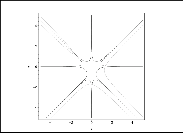
Figure 3. Curves of period three orbits and eigenvalues $|\lambda_{3}(x,y)|=1$.

Figure 5. Curves of period $1$, $2$ and $4$ orbits on the $(x,y)$-plane.

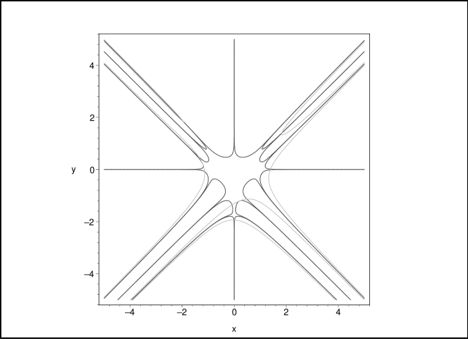
Figure 7. Curves of period four orbits and eigenvalues $|\lambda_{4}(x,y)|=1$.

Figure 8. Curves of period four orbits and eigenvalues $|\lambda_{4}(u,v)|=1$.

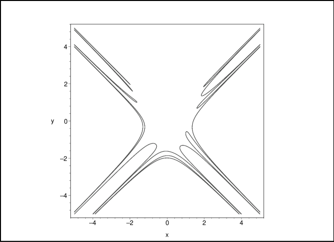
Figure 9. Curves of period $5$ orbits on the $(x,y)$-plane.

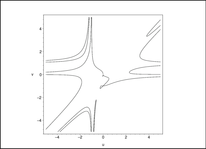
Figure 10. Curves of period $5$ orbits on the $(u,v)$-plane.

Figure 11. Curves of period five orbits and eigenvalues $|\lambda_{5}(x,y)|=1$.

Figure 12. Curves of period five orbits and eigenvalues $|\lambda_{5}(u,v)|=1$.

Figure 13. Curves of period $1-5$ orbits on the $(x,y)$-plane.

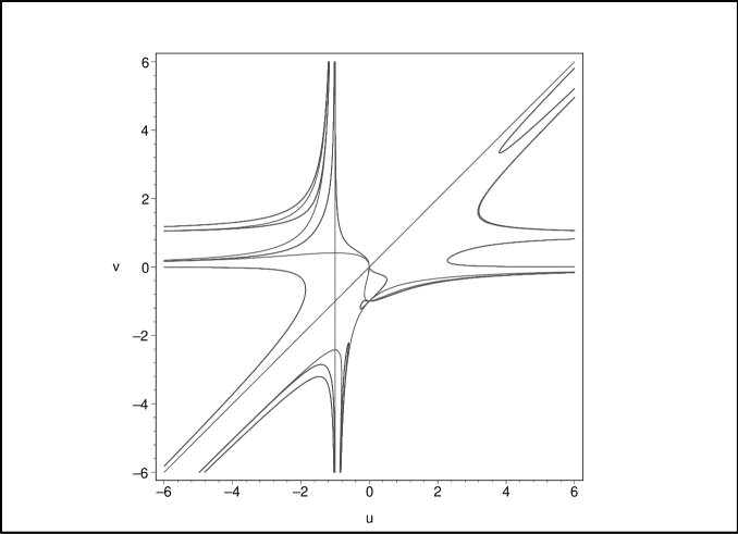
Figure 14. Curves of period $1-5$ orbits on the $(u,v)$-plane.

Figure 17. The bifurcation diagram of the function $F(x,y)=(y,y^{2}+y-x^{2})$.

Figure 18. The bifurcation diagram of the function $G(u,v)$.

References

- [1] Beardon Alan F.: Iteration of rational functions, Springer-Verlag, New York, (1991).
- [2] Blanchard Paul: Complex analytic dynamics on the Riemann Sphere, Bulletin of the American mathematical society, volume 11, Number 1, (1984).
- [3] Brown A.: Equations for periodic solutions of a logistic difference equation, Australian mathematical Society, (1981), no. 1, 78–94.
- [4] Collet Pierre, Eckmann Jean-Pierre: Iterated maps on the interval as dynamical systems, Springer, Boston/New York, (1980).
- [5] Erkama Timo: Periodic orbits of quadratic polynomials, Bull London Math. Soc., 38, (2006), s. 804-814.
- [6] Flynn E. V., Poonen Bjorn, Schaefer Edward F.: Cycles of quadratic polynomials and rational points on a genus-2 curve, Duke mathematical journal, vol.90, no.3, (1997).
- [7] Lyubich Mikhail: The quadratic family as a qualitatively solvable model of chaos, American mathematical society, volume 47, Number 9, (2000).
- [8] Morton Patrick: Arithmetic properties of periodic points of quadratic maps II, Acta Arithmetica, LXXXVII, (1998).
- [9] Peitgen Heinz-Otto, Jurgens Hartmut, Saupe Dietmar: Chaos and Fractals, Springer-Verlag, New York, (1992).
- [10] Stephenson John: Formulae for cycles in the Mandelbrot set, Physica A 177, (1991), s. 416-420.
- [11] Stephenson John, Ridgway Douglas T.: Formulae for cycles in the Mandelbrot set II, Physica A 190, (1992), s. 104-116.