Growth and dissolution of spherical density enhancements in SCDEW cosmologies.

Abstract:

Strongly Coupled Dark Energy plus Warm dark matter (SCDEW) cosmologies are based on the finding of a conformally invariant (CI) attractor solution during the early radiative expansion, requiring then the stationary presence of $\sim 1\,\%$ of coupled–DM and DE, since inflationary reheating. In these models, coupled–DM fluctuations, even in the early radiative expansion, grow up to non–linearity, as shown in a previous associated paper. Such early non–linear stages are modelized here through the evolution of a top–hat density enhancement. As expected, its radius $R$ increases up to a maximum and then starts to decrease. Virial balance is reached when the coupled–DM density contrast is just 25–26 and DM density enhancement is $\cal O$$(10\,\%)$ of total density. Moreover, we find that this is not an equilibrium configuration as, afterwards, coupling causes DM particle velocities to increase, so that the fluctuation gradually dissolves. We estimate the duration of the whole process, from horizon crossing to dissolution, and find $z_{horizon}/z_{erasing}\sim 3\times 10^{4}$. Therefore, only fluctuations entering the horizon at $z\lesssim 10^{9}$–$10^{10}$ are able to accrete WDM with mass $\sim 100\,$eV –as soon as it becomes non–relativistic– so avoiding full disruption. Accordingly, SCDEW cosmologies, whose WDM has mass $\sim 100\,$eV, can preserve primeval fluctuations down to stellar mass scale.

1 Introduction

LCDM cosmologies are highly performing effective models. What be the physics behind the LCDM paradigm, this is the question. A set of options descend from assuming General Relativity violation, at large scales or low densities. But listing these and other options (see e.g. [1]) is out of our scopes, as here we focus on a peculiar variant of a specific option, that Dark Energy (DE) is a scalar field $\Phi:$ when self–interacting, infact, a scalar field can exhibit a negative pressure approaching its energy density ($|p_{\Phi}|\sim|\rho_{\Phi}|$) [2]. Within the frame of these models we then treat a specific question concerning SCDEW (Strongly Coupled Dark Energy plus Warm dark matter) cosmologies [3].

These cosmologies, widely discussed also in the previous associated paper (hereafter BMM) [4], are however quite a peculiar branch of scalar field models, being based on a conformally invariant (CI) attractor solution of background evolution equations, holding all through radiative eras, and allowing then for significant $\Phi$ and Dark Matter (DM) densities. Let us recall soon that such DM is coupled to DE and distinct from warm–DM, although viable models, discussed in BMM, allow DM components to share several features, as Higgs’ masses $m_{w}$ and $\tilde{\mu}\equiv m_{c}$ (for WDM and coupled DM, respectively) and primeval densities.

The focus of this paper is then on the early evolution of spherical density enhancement in SCDEW cosmologies. In fact, besides of being peculiar for the behavior of background components, they also exhibit specific features in fluctuation evolution and, in this paper, we show that coupled–DM fluctuations grow, indipendently of other components, and approach non–linearity well before all of them. By adopting a spherical top–hat model, we then follow them in the non–linear stages, until the virialization condition is fulfilled, so that the sphere is should stabilize at a given radius $R$ and density contrast $\Delta$. Somehow unexpectedly, however, such virial equilibrium condition is not permanent and the sphere seems doomed to total dissipation; all that occurs through radiative eras and will be probably end up as soon as other components are able to take part to the spherical growth.

More in detail, here we shall quantitatively follow the evolution of coupled–DM fluctuations until their (temporary) virialization (phase I) , also testing how results depend on the redshift when the horizon reaches the fluctuation size, and the amplitude the fluctuation has then. The dependence on the model parameters will be also partially explored. What is expected to happen later (phase II) is harder to explore analytically, and our aim is just to give an order of magnitude for the time taken by dissipation.

Our final aim amounts to approach a determination of the low–mass transfer function in SCDEW cosmologies, over scales that linear algorithms are unable to treat. In particular we aim at constraining the minimal scale for fluctuation survival, in SCDEW models. According to our approach, such scale lays in the large stellar mass range. Let us outline that it should be so in spite of DM particles sharing a (Higgs) mass $\cal O$$(100\,$eV).

From a quantitative side it is then worth recalling that the early intensity of DM–$\Phi$ coupling, in SCDEW models, is fixed by an interaction parameter

$$\beta=b\sqrt{16\pi/3}$$ (1)

expected to be $\cal O$$(10)$. The early density parameters,

$$\Omega_{c}=\Omega_{\Phi}/2=1/2\beta^{2}~{},$$ (2)

for coupled DM and $\Phi$, keep then a constant value through radiative eras, as both components expand $\propto a^{-4}$, just as radiative components.

Let us then outline soon that we shall use the background metric

$$ds^{2}=a^{2}(\tau)(d\tau^{2}-d\lambda^{2})$$ (3)

$\tau$ being the conformal time and $d\lambda$ the line element.

The primeval CI expansion is then broken by the acquisition of the tiny Higgs’ masses at the electroweak (EW) scale. WDM and the spinor field $\psi$ yielding coupled DM, in particular, are supposed to acquire a mass $\cal O$$(100\,$eV), intermediate between light quark, electrons, and neutrinos. The effective mass of the $\psi$ field, below the Higgs’ scale, then reads

$$m_{eff}=g_{h}m_{p}\exp[-(b/m_{p})(\Phi-\Phi_{p})]+\tilde{\mu}~{}.$$ (4)

Here $b$ coincides with the coupling in eq. (1), $\Phi_{p}$ is the value of the scalar field extrapolated to the Planck time according to the CI solution (even though unlikely to hold so early), $m_{p}$ is the Planck mass. During the CI expansion, $m_{eff}$ is given just by the first term of the expression (4), while $\Phi-\Phi_{p}=\tau_{p}/\tau~{}.$ Accordingly, in such era

$$m_{eff}\propto\tau^{-1}~{},$$ (5)

such behavior being gradually violated when the term $\tilde{\mu}$ acquires relevance. Let us however add that the value of $g_{h}$ enters quantitative results only through the ratio

$${\cal R}={\tilde{\mu}/(g_{h}m_{p})}$$ (6)

taken here as effective parameter, so that we can fix $g_{h}=2\pi$ as in BMM.

It is also worth defining $C=b/m_{p}$ and outline that the appearence of a Higgs’ mass bears another consequence, a progressive weakening of the effective DM–$\Phi$ coupling; infact, as explained in detail in BMM,

$$C_{eff}={C\over 1+{\cal R}\exp[C(\Phi-\Phi_{p})]}$$ (7)

so that, as soon as the dynamical (logarithmic) scalar field growth makes $\Phi\sim\Phi_{p}-\log{\cal R}/C$, the effective coupling weakens, and we expect $\beta_{eff}=\cal O$$(0.1)$ at the present time.

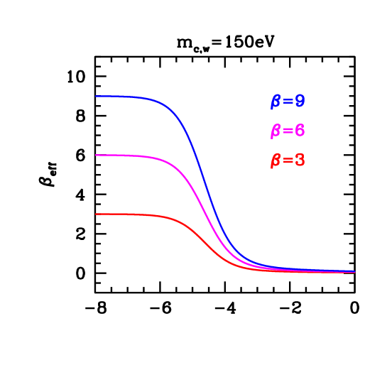
Figure 1: Scale dependence of the effective coupling in SCDEW cosmologies with $m_{c,w}=150\,$eV for various couplings $\beta$.

Accordingly, at $\tau<\tau_{H}$ ($T>T_{H}\sim 200\,$GeV, $z>z_{H}\sim 8\times 10^{14}$), a full CI holds (the suffix _H refers to Higgs’ mass acquisition at the EW scale).

Later on, at $\tau>\tau_{H}$ ($T<T_{H}\sim 200\,$GeV, $z<z_{H}\sim 8\times 10^{14}$), CI is violated; however, being $\tilde{\mu}\ll T_{H}$, a long period of effective CI expansion still occurs. Figure 1 shows the gradual end of such effective CI expansion, occurring quite late even for a fairly large value of $\tilde{\mu}\equiv m_{c,w}$, for several $\beta$ values. These behaviors are worked out from dynamical background equations.

The linear evolution of density fluctuations is widely discussed in BMM. The peculiar result, which is the starting point of this work, is that coupled–DM fluctuations exhibit an almost $\beta$ indipendent growth. In a synchronous gauge, it begins outside the horizon, accelerating when fluctuations pass through it, and persisting afterwards ($\tau\gg\tau_{hor}$), when the relativistic regime is over. It is so all through the CI expansion period, as well as early afterwards: in no case, after $\tau_{hor}$, coupled–DM fluctuations are subject to stagflation. This occurs in spite of coupled–DM being a fraction $\cal O$$(1\,\%)$ of the cosmic materials and while the other components either freely stream, if uninteracting, or begin sonic oscillations. The reason why this occur is recalled in the next Section.

Then, by using the linear program discussed in BMM, we appreciate that coupled–DM fluctuations, with amplitude $\cal O$$(10^{-5})$ at $\tau_{hor}$, reach an amplitude $\sim 0.1$ at $\tau_{nl}\sim 500\times\tau_{hor}$. Non–linear effects start then to be significant. Afterwards, at $\tau\sim 2$–$3\times 10^{3}\tau_{hor}$, it would then be $\langle\delta_{c}\rangle\sim 1$, yielding $\delta\rho_{c}\gtrsim\rho_{c}$; linear results are then meaningless.

In this regime, we can achieve a reasonable insight on the actual fluctuation evolution by following the behavior of (admittedly unlikely) spherically symmetric density enhancements. Such approach, in a different context, allows us to predict, e.g., the mass functions of real physical systems, as galaxy clusters; it is so because the approach yields a realistic clock of fluctuation growth and a schematic picture of their fate (see, e.g., [5]).

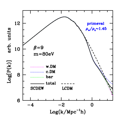
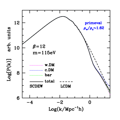
Figure 2: Linear spectra of the models used in this work, compared with LCDM spectra. The ratios between warm and coupled DM component densities, during the late CI expansion, is shown at the top right in blue. In both models we have a slight power deficit (up to a factor $\cal O$$(3)$) in the Lyman–$\alpha$ cloud region, while LCDM amplitude is recovered around average galactic scales. In principle, such increased amplitude means an earlier formation of structures on subgalactic scales.

However, at variance from what is done in the cited case, when we start following the evolution of a fluctuation, here we shall not assume it to expand within the Hubble flow, but work out its growth rate from the linear regime. Results are then nearly independent from the selected initial density contrast $\Delta_{c}=1+\delta_{c}$ if $\delta_{c}<10^{-2}$.

Most results of this paper are obtained by using 2 specific SCDEW models: either $\beta=9$ and $m\equiv m_{w}=m_{c}=80\,$eV (model 9) or $\beta=12$ and $m\equiv m_{w}=m_{c}=115\,$eV (model 12). In Figure 2 we show their $z=0$ linear spectra, as obtained from our linear algorithm, discussed in BMM. In all models, at $z=0$, $\Omega_{b}=0.045$, $\Omega_{\Phi}=0.70$, $h=0.685$, with the usual meaning of symbols. Furthermore we suppose $T_{0}=2.726\,$K and a primeval helium abundance $Y_{He}=0.24\,.$ Units yielding $c=\hbar=1$ are taken all through the paper.

The plan of the paper is as follows: In the next Section we derive the equations needed to follow the density enhancement evolution until virialization (phase I). In Section 3, we shall tentatively extend the analytical treatment to the evolution after it (phase II). In Section 4, numerical results will be shown. Section 4 contains a discussion of the results found.

2 Fluctuation evolution in the early Universe

All through this paper, the expressions (4) and (7) for DM particle mass and coupling will be used. Accordingly, we shall never deepen in the fully CI regime. This is not a problem, however, as the density enhancement behaviors, found for the smallest $\tau_{hor}$ considered, are quantitatively identical to those holding for $\tau_{hor}<\tau_{H}$. There exist, in fact, a long period of effective CI regime, when CI violations are so small to yield a negligible influence; see below for more details on this point.

2.1 A top–hat fluctuation in the early Universe

Let us then consider a spherical top–hat overdensity, entering the horizon with an amplitude $\delta_{c,hor}$, in the very early Universe.

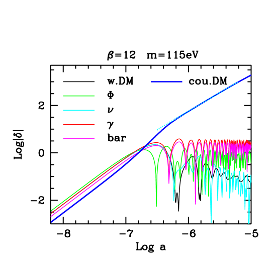
Figure 3: Typical linear evolution of linear density fluctuations close to horizon (the scale considered corresponds to $k=30\,h\,$Mpc^-1). The non–relativistic (linear) regime is approached when the cyan bended dotted line is attained (steepness $\delta_{c}\propto a^{1.6}$). The main parameters of the cosmology used are indicated at the top of the Figure, but most results are substantially model independent.

In this work we shall assume that $\delta_{c,hor}>0$ and, mostly, $\simeq 10^{-5}$, its top likelihood value. We expect fluctuations to exhibit a Gaussian distribution, so that different (namely greater) $\delta_{c,hor}$ values, although unlikely, are also possible. Our treatment however holds only for $\delta_{c,hor}$ values small enough to allow $\delta_{c}$ to enter a non–linear regime only when already non–relativistic. The case of $\delta_{c}$ entering the non–linear regime when still relativistic, in the frame of SCDEW models, relevant for predictions on primeval Black Holes [7], will be discussed elsewhere.

The critical point, however, is clearly illustrated in Figure 3. Here we show the fluctuation growth, as derived from our linear program, close to the horizon. At the horizon crossing, being in the relativistic regime, coupled DM fluctuations exhibit a significantly upgraded growth rate. When sufficiently inside the horizon, the growth rate slows down, and $\delta_{c}\propto a^{\alpha}$ with $\alpha\simeq 1.6\,.$ The Figure also shows that coupled DM fluctuations exhibit a steady growth while the other component fluctuations undergo free streaming or enter a sonic regime with stationary amplitude.

This behavior can be easily understood, at least in the non–relativistic regime, by taking into account the treatment in [8], concerning the evolution of coupled–DM overdensities. Let us outline that this treatment, specifically devised to perform N–body simulations, holds both in the linear and in the non–linear regime. In that work, aiming to perform N–body similations of coupled–DE models, it is shown that coupling effects are equivalent to: (i) An increase of the effective gravitational push acting between DM particles, for the density fraction exceeding average, while any other gravitational action remains normal. The increased gravitation occurs as though $G=1/m_{p}^{2}$ becomes

$$G^{*}=\gamma\,G~{}~{}~{}~{}{\rm with}~{}~{}~{}~{}\gamma=1+4\beta^{2}/3$$ (8)

($m_{p}:$ Planck mass). (ii) As already outlined in eqs. (4) and (5), coupled–DM particle masses progressively decline. This occurs while the second principle of dynamics still requires that ${\bf f}={\bf p}^{\prime}$ (here the prime indicates differentiation in respect to the ordinary time $t$). This yields the dynamical equation

$${d{\bf v}\over d\,t}={{\bf f}\over m_{eff}}+\left|m_{eff}^{\prime}\over m_{eff}\right|{\bf v}~{},$$ (9)

i.e. an extra–push to particle velocities, adding to the external force f.

It should be outlined that, once eqs. (8) and (9) are applied, the whole effects of coupling are taken into account; in particular, the (small) $\Phi$ field perturbations cause no effect appreciable at the Newtonian level (see again [8]). This is true even in the presence of extreme DM density contrasts, as those found in the halos produced by N–body simulations, and, even more, in the linear case considered here.

The self–gravitational push due to $\delta_{c}$ is then $\propto G^{*}\rho_{c}\delta_{c}=G\rho_{cr}(2/3)\delta_{c}\times(1+3/4\beta^{2})$, with the last factor exceeding unity just by $\sim 1\,\%$ for $\beta=\cal O$$(10)$. Henceforth, coupled DM fluctuations, in the non–relativistic regime, grow as though concerning the total cosmic density $\rho_{cr}$, at least. The slightly reduced amplitude, in fact, is overcompensated by the extra–push and, as previously outlined, the linear program gives evidence of a grows $\propto a^{\alpha}$ with $\alpha\sim 1.6\,.$

Within this context, we can schematically describe the evolution of a spherical top–hat density enhancement of amplitude $\delta_{c}$. The fluctuation initially expands according to linear equations, but, as soon as $\delta_{c}\gtrsim 10^{-2}$–$10^{-1}$, non–linear effects become no longer negligible. At this stage, the radius $R$ of the top–hat, growing more slowly than the scale factor $a$, reaches a maximum value $R_{top}$ and then starts to decrease. Eventually, however, inner kinetic and potential energies reach a virial balance, when the sphere has a radius $R_{vir}$.

Let us then recall that, in the framework of a “standard CDM” cosmology, there exist an analytical (parametric) solution of the equations ruling the evolution of a spherical top–hat overdensity. The evolution of a spherical overdensity in a coupled–DE model, with $\beta\ll 1\,,$ was considered by [6]. The key issue was then that both baryons and coupled DM fluctuations grow, but at different rates: the DM component is faster in reaching maximum expansion and starts to recontract before baryons. It is then necessary to share the top–hat fluctuation into shells, which gradually compenetrate. The number of shells needed is determined by the precision wanted. In Figure 3 we directly see that we are now dealing with a case when only coupled–DM fluctuations grow. The equations ruling $R$ evolution are then similar to those obtained in [6], with the welcomed difference that we need no subdivision into spherical shells.

The relation between the comoving sphere radius $c=R/a$ and the density contrast $\Delta_{c}=1+\delta_{c}$ then reads

$$\Delta_{c}=1+\delta_{c}=\Delta_{c,r}c_{r}^{3}/c^{3}~{},$$ (10)

as the subscript _r refers to a suitable reference time; accordingly, by assuming $\delta_{c}\propto\tau^{\alpha}$,

$${\dot{c}\over c_{r}}=-{\alpha\over 3}{\delta_{c,r}\over\Delta_{c,r}}{1\over\tau}~{};$$ (11)

this relation allows us to chose arbitrarily the time $\bar{\tau}$, during the linear regime, when we start to use $c$ instead of $\delta_{c}$ to follow the top–hat dynamics.

2.2 Dynamical equation

In strict analogy with eq. (9) in [6], the evolution of the overdensity then follows the equation

$$\ddot{c}=-\left({\dot{a}\over a}-C\dot{\Phi}\right)\dot{c}-\gamma G{1\over ac^{2}}[M(<R)-\langle M(<R)\rangle]~{}.$$ (12)

Here, as in eq. (11), derivatives are taken in respect to the conformal time $\tau$; $\Phi$ is the background value of the scalar field. Furthermore, $M(<R)$ is the actual mass within $R$, while $\langle M(<R)\rangle$ is the average mass in a sphere of radius $R$, but, if assuming all components but coupled–DM to be unperturbed, we only need evaluating

$$G\langle M_{c}(<R)\rangle=G{4\pi\over 3}\rho_{cr}\Omega_{c}a^{3}c^{3}={\Omega_{c}\over 2}{h_{2}\over\tau^{2}}a\,c^{3}$$ (13)

with

$$h_{2}={8\pi\over 3}G\rho_{cr}a^{2}\tau^{2}$$ (14)

being close to unity, during the effective CI expansion and exactly unity at $\tau<\tau_{H}$, when also $\Omega_{c}\equiv 1/2\beta^{2}$. However, at later times, when $\beta$ must be replaced by $\beta_{eff}$, no similar relation holds.

Let then $\bar{\Delta}$ be the density contrast at the time $\bar{\tau}$, so that

$${1\over\bar{\Delta}}GM_{c}(<R)=G{4\pi\over 3}m_{eff}(\tau)\,\bar{n}_{c}\,\bar{a}^{3}\bar{c}^{3}~{}.$$ (15)

Here $n_{c}$ is the number density of coupled–DM particles, whose mass $m_{eff}$ is given by eq. (4) (all “barred” quantities refer to the “initial” time $\bar{\tau}$). As $n_{c}a^{3}$ is constant in time, it is also

$${1\over\bar{\Delta}}GM_{c}(<R)=G{4\pi\over 3}m_{eff}\,n_{c}~{}a^{3}\bar{c}^{3}=G{4\pi\over 3}\rho_{cr}\Omega_{c}~{}a^{3}\bar{c}^{3}={\Omega_{c}\over 2}{h_{2}\over\tau^{2}}a\,\bar{c}^{3}~{}.$$ (16)

Accordingly, by setting $\Delta M_{c}=[M_{c}(<R)-\langle M_{c}(<R)\rangle]$, we have

$$G~{}\Delta M_{c}={\Omega_{c}\over 2}{h_{2}\over\tau^{2}}a\bar{c}^{3}\left({\bar{\Delta}}-x^{3}\right)~{}~{}~{}{\rm with}~{}~{}~{}x=c/\bar{c}$$ (17)

so that

$${G\over ac^{2}}[M(<R)-\langle M(<R)\rangle]={\Omega_{c}\over 2}{h_{2}\over\tau^{2}x^{2}}\bar{c}\left({\bar{\Delta}}-x^{3}\right)~{}.$$ (18)

In turn, the difference $h_{0}=\dot{a}/a-C\dot{\Phi}$ exactly vanishes, during the early CI expansion, both terms being then $1/\tau$. As the background density of coupled DM fulfills the equation

$$\dot{\rho}_{c}+3(\dot{a}/a)\rho_{c}=-C\rho_{c}\dot{\Phi}$$ (19)

it is however worth keeping into account that

$$h_{0}=-C\dot{\Phi}+{\dot{a}\over a}={\dot{\rho}_{c}\over\rho_{c}}+4\,{\dot{a}\over a}~{},$$ (20)

as this allows an easier numerical evaluation of $h_{0}$. Altogether, eq. (12) also reads

$$\ddot{x}=-h_{0}\dot{x}-h_{1}\left(\bar{\Delta}-x^{3}\right){1\over u^{2}x^{2}}$$ (21)

with

$$h_{1}={1\over 2}\gamma\Omega_{c}h_{2}~{},~{}~{}~{}$$ (22)

and $u=\tau/\bar{\tau}$, while, at variance from elsewhere, dots here indicate differentiation in respect to $u$. In eq. (21), describing a process due to self–gravity, the gravitational constant no longer explicitly appears, being reabsorbed in the definition of $h_{2}$ (eq. 14) and then in $h_{1}$.

Let us finally outline that, until we are close to the CI expansion, the coefficient

$${1\over 2}\gamma\Omega_{c}=\left(1+{4\over 3}\beta^{2}\right){1\over 4\beta^{2}}={1\over 3}+{1\over 4\beta^{2}}$$ (23)

keeps close to 1/3, for reasonable $\beta$’s (see however Figure 4). Eq. (21) however holds both then (when also $h_{2}=1$) and when CI is abandoned, so that $h_{1}$ can become even quite different from 1/3 .

Figure 4: During the CI expansion the coefficient $h_{1}={1\over 2}\gamma\Omega_{c}$ is almost $\beta$ independent.

2.3 Virialization

Numerical solutions of eq. (21) yield the expected growth and successive recontraction of the radius $R$ of top–hat density enhancements, as well as the gradual increase of the density contrast $\Delta_{c}$ in respect to the average coupled–DM density $\rho_{c}$; it is also clear that an ideal top–hat would expand and recontract, according to the above expressions, down to a relativistic regime. Top–hat fluctuations were however considered because their equations of motions are integrable and provide an insight into the real timing of true fluctuation evolution. Virialization is then the successive step assumed to occur, because real motions are unordered and exact sphericity breaks down when we pass from expansion to recontraction.

To establish the conditions for virial balance, we then need the expressions of the kinetic and potential energy for the sphere. In accordance with [6], the kinetic energy expression is rather simple to obtain and reads

$$T_{c}(R)={3\over 10}M_{c}{R^{\prime}}^{\,\,2}~{},$$ (24)

as the factor 3/10 derives from integration on a sphere. Here, the prime indicates differentiation with respect to ordinary time, so that $R^{\prime}=(a\,\dot{c}+\dot{a}\,c)/a=\dot{c}+(\dot{a}/a)\,c$, if dots indicate differentiation with respect to $\tau$; by using eq. (14), we then have

$$2\times{5\over 3}{T_{c}\over M_{c}}={\bar{c}^{2}\over\bar{\tau}^{2}}\left(\dot{x}+{h_{2}^{1/2}\over u}x\right)^{2}~{},$$ (25)

dots indicating here differentiation in respect to $u$.

The potential energy is then made of two terms, arising from DM fluctuation interacting with DM background and all backgrounds interacting with themselves. Therefore, in agreement with [6] where, however, the only unperturbed background was DE,

$${U_{c}(R)\over M_{c}}=-{3\over 5}G{[\langle M_{c}\rangle+\gamma\Delta M_{c}]\over R}-{4\pi\over 5}G\rho_{back}R^{2}=-{3\over 5}\gamma G{\Delta M_{c}\over R}-{4\pi\over 5}G\rho_{cr}R^{2}~{}.$$ (26)

By using the expression (17) for $G\,\Delta M_{c}$, we then have

$$-{\gamma G\over R}\Delta M_{c}=-{\gamma\Omega_{c}\over 2}{h_{2}\over\tau^{2}x}\bar{c}^{2}(\bar{\Delta}-x^{3})=-{\bar{c}^{2}\over x}{h_{1}\over\tau^{2}}(\bar{\Delta}-x^{3})$$

while

$$-{4\pi\over 3}G\rho_{cr}R^{2}=-{8\pi\over 3}G\rho_{cr}a^{2}{c^{2}\over 2}=-{\bar{c}^{2}\over\tau^{2}}{h_{2}x^{2}\over 2}$$

so that

$${5\over 3}{U_{c}(R)\over M_{c}}=-{\bar{c}^{2}\over\tau^{2}}\left[{h_{2}x^{2}\over 2}+{h_{1}\over x}(\bar{\Delta}-x^{3})\right]$$ (27)

Virilization is then obtainable by requiring that

$$2\times{5\over 3}{T_{c}\over M_{c}}+{5\over 3}{U_{c}\over M_{c}}=0$$ (28)

or, by using the expression (25) and (27) hereabove,

$$(u\dot{x}+{h_{2}^{1/2}}x)^{2}-h_{1}(\bar{\Delta}/x-x^{2})-h_{2}x^{2}/2=0~{}.$$ (29)

From the $c_{v}$ and $\tau_{v}$ values fulfilling this equation, we then derive tha virial radius $R_{v}=c_{v}a_{v}$. Neither the equation of motion, nor this expression, are suitable for analytical treatment.

3 After virialization

In order to better understand the physical sense of the virialization condition, let us assume that the CI expansion regime holds and, in particular, $h_{0}=0$ and $h_{2}=1$. According to eqs. (24) and (26), the top–hat virial then reads

$${5\over 3}{Vir\over M_{c}}=\langle v^{2}\rangle-{4\pi\over 3}G\rho_{cr}\left(\gamma\Omega_{c}\Delta+{1\over 3}-\Omega_{c}\right)R^{2}~{},$$ (30)

once we replace ${R^{\prime}}^{2}=\langle v^{2}\rangle$, as we expect particle velocities yielding coherent contraction to turn into randomly distributed speeds.

It is then convenient to multiply this relation by $m_{eff}^{2}$ and outline the vanishing of the virial through the approximate relations

$$\langle p^{2}\rangle=\gamma G{N_{c}m_{eff}^{3}\over R_{v}}={4\pi\over 3}\gamma G\rho_{cr,v}\Omega_{c}\Delta_{v}R_{v}^{2}m_{eff}^{2}={1\over 4t_{v}^{2}}h_{1}\Delta_{v}R_{v}^{2}m_{eff}^{2}~{},$$ (31)

($N_{c}$ is the total number of coupled–DM particles, yielding a total mass $N_{c}m_{eff}$) so to take easily into account that, in spite of $m_{eff}$ progressive decrease, the square averaged momentum $p_{v}^{2}\equiv\langle p^{2}\rangle$ is however expected to keep constant. All quantities with index _v refer to virialization. The relation (31) is readily understandable as a balance between twice the average particle kinetic energy $\langle(p^{2}/m_{eff})\rangle$ and its potential energy in respect to coupled–DM (only), just as in the process of virialization of a top–hat matter density enhancement after matter–radiation decoupling (PS–case).

In both cases, once $R_{v}$ is reached, the recontraction process is not immediately discontinued and a stationary configuration is reached after a few oscillations; since $t_{v}$, however, the average particle momentum is expected to keep $p_{v}$. The point is then that the average particle momentum, at any $t>t_{v}$, exceeds the virial equilibrium momentum

$$p_{v}^{2}(t)=p_{v}^{2}(\tau_{v}/\tau)^{3}=p_{v}^{2}(t_{v}/t)^{3/2}~{},$$ (32)

because of the progressive decrease of $m_{eff}\propto\tau^{-1}$. Should all particle momenta coincide with $p_{v}$, a global free streaming would follow, and the characteristic time for a full dissolution would be the crossing time $t_{cross}=R_{v}/v_{v}$ (here $m_{eff}v_{v}=p_{v}$). The distribution of particle momenta, however, can be expected to be close to a maxwellian

$$f(p/p_{t})\equiv f(x)={4\over\sqrt{\pi}}x^{2}e^{-x^{2}}~{},$$ (33)

with $p_{t}=\sqrt{2/3}\,p_{v}$ being the distribution top. Evaporation will then start from fastest particles and, in principle, it is possible that the momentum they carry away allows a sufficient average momentum decrease, so that

$$\langle p^{2}(t)\rangle=p_{v}^{2}{N_{c}(\tau)\over\bar{N}_{c}}\left(\tau_{v}\over\tau\right)^{3}=p_{v}^{2}{N_{c}(t)\over\bar{N}_{c}}\left(t_{v}\over t\right)^{3/2}~{}.$$ (34)

Let us outline that $\langle p^{2}(t)\rangle$ is required to decrease faster than $p_{v}^{2}(t)$, as the potential energy to balance also decreases when the total number of particles ($N_{c}$) declines. By dividing both sides of eq. (34) by $p_{v}^{2}$ and taking into account the particle distribution, we then have

$${p_{t}^{2}\over p_{v}^{2}}{\int_{0}^{\alpha}dx\,x^{2}f(x)\over\int_{0}^{\alpha}dxf(x)}={2\over 3}{\int_{0}^{\alpha}dx\,x^{2}f(x)\over\int_{0}^{\alpha}dx\,f(x)}=\left(1\over 1+t_{\alpha}/t_{v}\right)^{3/2}\int_{0}^{\alpha}dx\,f(x)~{};$$ (35)

here we took into account that the Boltxmann distribution is normalized to unity; we also set $t=t_{v}+t_{\alpha}$, so to outline the time $t_{\alpha}$ when particles with momenta $p>\alpha\,p_{t}$ were allowed to evaporate. We can also define

$$F(\alpha)\equiv{2\over 3}{\int_{0}^{\alpha}dx{4\over\sqrt{\pi}}x^{4}e^{-x^{2}}\over\left[\int_{0}^{\alpha}dx{4\over\sqrt{\pi}}x^{2}e^{-x^{2}}\right]^{2}}=\left(1\over 1+t_{\alpha}/t_{v}\right)^{3/2}$$ (36)

and seek the value $\alpha_{m}$ minimizing $F(\alpha)$; the point is that, after the most rapid particles have evaporated, the momentum decrease granted by further slower particle evaporation is beaten by the potential energy decrease due to the outflow of particles belonging to the bulk of the distribution.

The process should then not proceed beyond $t_{ev}\equiv t_{\alpha_{m}}$, that we dubb evaporation time; i.e., in order to grant a “long life” to the residual density enhancement, it should be $t_{cross}\ll t_{ev}$. This would allow only particles with high momentum to outflow, even though initially well inside the enhancement. Furthermore, $t_{cross}$ is also the order of magnitude of the time needed for rearranging particle momentum distribution, when the fastest particles have outflown, so to recover a Bolzmann distribution, and allow for further fast particle evaporation.

According to eq. (31), it is then easy to see that

$${t_{cross}\over t_{v}}={2\over(h_{1}\Delta_{v})^{1/2}}~{}.$$ (37)

Notice that eq. (37) holds also in the PS–case provided we replace $h_{1}$ by $\Omega_{m}/2$ (matter density parameter). A fair comparison between evaporation and crossing times then requires that $\Delta_{v}$ is known.

Before passing to a numerical treatment of the problem, let us however outline that the point we still debate is the time–scale for the top–hat dissolution, which is however expected to occur anyhow. Should however be $t_{ev}<t_{cross}$, we face a situation when the dissolution is almost immediate, taking just a few $t_{cross}$; i.e., the time needed to settle in virial equilibrium, in the PS–case.

4 Numerical treatment

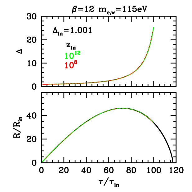
Figure 5: Top hat radius and density contrast evolution for the model 12. In abscissa, the conformal time $\tau/\tau_{in}$ is substantially coincident with $a/a_{in}$. Both $z_{in}=10^{12}$ and $10^{8}$ are considered, but the curves essentially overlap. The only tenuous difference is a slight shift for the value of the final density contrast. In the bottom plot, the eventual evolution of $R$, assuming virialization not to occur, is also shown down to $R=0$ (relativistic regime).

4.1 Phase I

Top–hat evolution, during the CI expansion, is fairly easily integrated, as the dynamical coefficients are then constant. We shall not report the results for this case, but only those obtained by setting the initial condition at $z_{in}=10^{12}$ and $10^{8}$. As a matter of fact, the former case yield results numerically coincident with those for $z_{in}>z_{H}$, while the very difference between $z_{in}=10^{12}$ and $10^{8}$ is quite small.

In Figure 5 we show the behaviors of the radius $R$ and the density contrast $\Delta$ vs. the conformal time $\tau$ for the model 12.

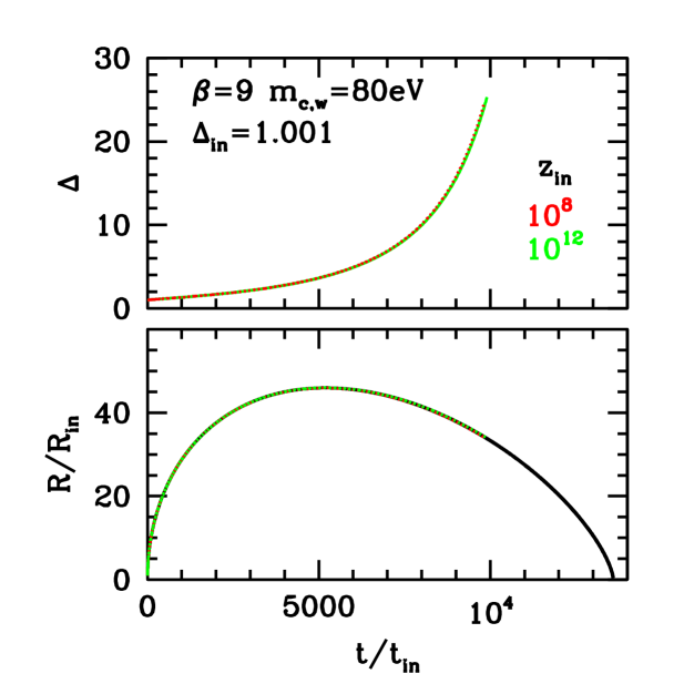
Figure 6: Top hat radius and density contrast evolution for the model 9. In abscissa, the ordinary time $t/t_{in}$. Also here the curves for $z_{in}=10^{12}$ and $10^{8}$ essentially overlap while, again, the only tenuous difference is a slight shift for the value of the final density contrast. In the bottom plot, as in the previous Figure, the eventual evolution of $R$, assuming virialization not to occur, is also shown down to $R=0$.

For model 9 we then rather show the evolution by using ordinary time in abscissa (figure 6).

As a matter of fact, it seems more significant to outline the different apparent behavior when the abscissa is changed, rather than the tiny model dependence.

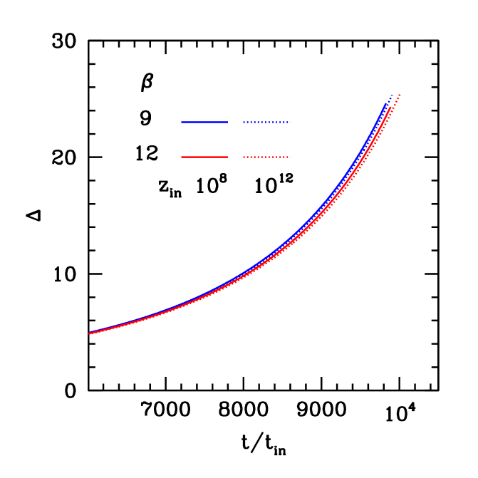
Figure 7: Blow up of the final part of the density contrast growth, before virialization, for both models and $z_{in}$.

.

In order to magnify the differences between models and $z_{in}$ values, where they exist, we however plot the final part of the density contrast increase, prior to virialization, in Figure 7. For the sake of completeness let us then provide the numerical values of the virial density contrasts. For $\beta=12$ they are 25.4 or 24.3 when $z_{in}=10^{12}$ or $10^{8}$, respectively, while, for $\beta=9$, the corresponding values are 25.3 or 24.6 . Let us also add that, if we start following the density contrast evolution when $\bar{\Delta}=1.1$, instead of 1.001, we obtain slightly smaller values: e.g., for $\beta=12$, they read 25.3 and 24.2, if the density contrast $\Delta_{c}=1.1$ is attained at $z_{in}=10^{12}$ or $10^{8}$, respectively. Non–linearity, when $\delta_{c}<0.1$, has quite a limited impact, not exceeding half percent.

This greater “initial” density contrast can be due to rare fluctuations entering the horizon already with a wider amplitude; the point is that we however reach a virial density contrast just marginally different from starting when $\Delta_{c}=1.001$; i.e., that non linearity effects are negligible for $\delta_{c}<0.1$. The procedure followed is therefore well approximated also if the relativistic regime due to horizon crossing ends up when the density contrast is already $\cal O$$(1.1)$. Such greater $\Delta_{c}$ at $z_{in}$, however, is not met just for exceptional fluctuations, being possibly due just to an earlier horizon crossing and, therefore, to fluctuations over smaller scales.

Let us rather outline that a final density contrast $\sim 25$–26 is “small”. As the fractional contribute of coupled DM to the overall density is $\Omega_{c}\sim 0.005$, it is clear that even $\Delta_{v}\Omega_{c}\sim 0.13$ is still far from unity: the total density enhancement, at virialization, does not exceed the overall density, as though still being in a quasi–linear regime. In turn, this strengthens the reliability of results obtained by neglecting density fluctuations in other components, when considering coupled–DM fluctuation evolution. Taking them into account could only yield a modest correction for final results.

It can also be significant to follow the evolution of the dynamical coefficient $h_{i}$. In Figure 8 we show them for the case $\beta=12$.

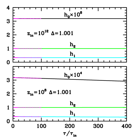
Figure 8: Dynamical coefficients for the model 12. At the l.h.s., the $\tau$ interval covered before virialization is dotted in magenta color. Notice also: (i) When $z_{in}=10^{12}$ all coefficient appear substantially constant, even behind the l.h.s. interval; on the contrary, for $z_{in}=10^{8}$ a slight time dependence is appreciable, namely for $h_{0}$. (ii) The difference of $h_{0}$ from nil rapidly increases when smaller $z_{in}$ values are considered; however, even $h_{0}\sim 10^{4}$ values yield no contribution to the actual $R$ evolution.

.

The behavior for $\beta=9$ does not exhibit significant differences.

In the Figure, the ranges of $h_{i}$ values used by the numerical integrator, before virialization, are outlined by magenta dots. Namely on such interval, $h_{i}$ variations are however quite small.

Notice however how $h_{0}$ increases when smaller $z_{in}$ values are considered; during the CI expansion, $h_{0}\equiv 0$; although so small, the values of $h_{0}\neq 0$ shown outline the exit from CI expansion. In spite of that, even $h_{0}\sim 10^{4}$ values yield no appreciable contribution to the numerical $R$ evolution.

Notice also that $h_{i}$ coefficient appear fully $\tau$ independent, for $z_{in}=10^{12}$; on the contrary, for $z_{in}=10^{8}$ a time dependence is appreciable; it is strongest for $h_{0}$, but, as earlier outlined, this bears no appreciable dynamical consequences.

4.2 Phase II

Once the density contrast $\Delta_{v}$ is known, the crossing time (37) can be soon evaluated, being $t_{cross}\simeq 0.7\,t_{v}$ (in the PS case, for $\Lambda$CDM, $t_{cross}\simeq 0.5\,t_{v}$).

In Figure 9 we report the $F(\alpha)$ dependence, showing that $F(\alpha_{m})\simeq 0.81$, so yielding

Figure 9: The dependence on $\alpha$ of the $F(\alpha)$ allows us to estimate down to which momentum ($\alpha\times p_{t}$) it is dynamically “convenient” that fast particles evaporate from the density enhancement, to ease a virial equilibrium recovery, in spite of $m_{eff}\propto\tau^{-1}$. The fast $F$ increase, when $\alpha$ shifts below $\sim 1.21$, arises because the bulk of the Boltzmann distribution is then supposed to outflow.

$t_{ev}=0.15\,t_{v}$. The conclusion is that, once the virial equilibrium condition is attained, the density enhancement is unable to settle on it. The expected downward and upward oscillations which, in the PS case, last $\sim t_{v}$, here are slightly longer and doomed to end up with a substantial particle free streaming.

A way to stabilize the virialized system can only exist if, during the fluctuation linear and/or non–linear growth, other cosmic component particles were allowed to accrete, as will be when the WDM component approaches derelativization.

5 Discussion

In a standard cosmological model with warm DM made of particles with mass $\sim 100\,$eV, the minimal fluctuation scale surviving free streaming is the scale entering the horizon at $z_{der}\sim 6\times 10^{\,5}(m_{w}/100\,{\rm eV})^{4/3}(\Omega_{w}h^{2})^{-1/3}$, so ranging about $2\times 10^{13}h^{-2}M_{\odot}$ and exceeding the size of the largest galaxies. The presence of coupled–DM in SCDEW models allows us to shift the critical redshift from $z_{der}$ to $\sim 10^{4}z_{der}$, so lowering by $\sim 12$–13 orders of magnitude the mass scale of the minimal surviving WDM fluctuation.

The peculiarity of SCDEW cosmologies, however, is that this is not due to an ad–hoc mechanism, being the unavoidable consequence of the previous expansion along an attractor, through modified radiative eras. SCDEW cosmologies, infact, are characterized by a substantial modification of such early expansion regime, i.e., the constant presence of coupled DM and $\Phi$, in fixed proportions, aside of standard radiative components.

The above result is obtained by studying the evolution of a top–hat density fluctuation in the late radiative era. Using a spherical fluctuation to work out the expected time scale of processes is not a new procedure. In a different context, it was first applied to predict the mass function of cosmic bounded structures, as galaxy clusters [5]. Results were excellent and, with suitable improvements, a similar approach is still in use.

When we treat a top–hat density enhancement of radius $R$, we find $R$ gradually slowing down its growth rate in respect to the scale factor $a$. Eventually, the $R$ increase stops and $R$ begins to decrease. After a suitable time, however, kinetic and potential energy reach a virial balance, so that we should expect equilibrium to be attained.

Here however comes the most peculiar feature of coupled–DM fluctuations: the virial condition is unstable. This is due to the progressive decrease of the coupled–DM particle mass $m_{eff}$, causing the increase of the kinetic energy $\sim p^{2}/m_{eff}$ if the momentum $p$ is conserved, and a symultaneous decrease of the depth of the potential well, roughly $\propto m_{eff}^{2}$.

As a consequence of these variations, the most rapid particles are expected to evaporate. We provided analytical tools to estimate evaporation effects and, as above outlined, estimated how long a significant density contrast can persist after virialization.

It is however legitimate to wonder how reliable can be estimates based on a spherical top–hat evolution. The physics described here, however, does not seem to need a sphericity assumption. Quite in general, coupled–DM particles, embedded in a fluctuation entering the horizon, are initially slow enough, so that their kinetic energy does not interefere with fluctuation growth. The evolution described by linear programs occurs under such conditions, but eventually causes a fast growth of coupled–DM fluctuations, in spite of their density being a small fraction of the total density. The reach of the non–linear regime, therefore, is independent from any spherical modeling.

We then expect that non–linearity produces significant energy jumps, and the possibility to transfer such potential energy jumps onto particle kinetic energy. Once particle momenta reach a significant level, particle velocities burst, aside of $m_{eff}$ decrease. Escape velocity could then be approached and overcame, and the heaten up coupled–DM could no longer be constrained in primeval inhomogeneities. The study of top–hat spherical fluctuations tries to model these events and, hopefully, to provide a reasonably reliable clock for them.

References

- [1] Amendola L. & Tsujikawa S., 2010, Cambridge Univ. Press, Dark Energy: theory & observations.
- [2] see, e.g., Ellis J., S. Kalara, K.A. Olive & C. Wetterich, 1989, Ph.Lett.B 228, 264; Ratra B. & Peebles P.J.E., 1988, PRD 37, 3406; Wetterich C., 1995, A&A 301, 321; Amendola L., 1999, PRD 60, 043501; Amendola L., 2000, PRD 62, 043511; Amendola L., Tocchini-Valentini D., 2002 PRD 66, 043528.
- [3] Bonometto S.A., Sassi G. & La Vacca G., 2012, arXiv:1206.2281 & JCAP08, 015 (2012); Dark energy from dark radiation in strongly coupled cosmologies with no fine tuning; Bonometto S.A. & Mainini R., 2014, arXiv:1311.6374 & JCAP03, 38, Fluctuations in strongly coupled cosmologies; Bonometto S.A., Mainini R. & Macció A.V., 2015, arXiv:1503.07875 & MNRAS 453, 1002 ; Strongly Coupled Dark Energy Cosmologies: preserving LCDM success and easing low scale problems I - Linear theory revisited; Macció A.V., Mainini R., Penzo C. & Bonometto S.A., 2015, arXiv:1612.05277 & MNRAS 453, 1371, Strongly Coupled Dark Energy Cosmologies: preserving LCDM success and easing low scale problems II - Cosmological simulations
- [4] Bonometto S.A., Mainini R. & Mezzetti M., 2017, arXiv ……. , Strongly Coupled Dark Energy with Warm dark matter vs. LCDM.
- [5] Press W.H. & Schechter P., 1974, ApJ 187, 425, Formation of Galaxies and Clusters of Galaxies by Self-Similar Gravitational Condensation
- [6] R. Mainini, 2005, PRD 72, 083514 & arXiv:astro-ph/0509318, Dark Matter-baryon segregation in the non-linear evolution of coupled Dark Energy model; see also: R. Mainini & S.A. Bonometto, 2006, PRD 74, 043505 & arXiv:astro-ph/0605621, Mass functions in coupled Dark Energy models;
- [7] see, e.g., Carr B.J., Kohri K., Sendouda Y. & Yokoyama J., 2009, arXiv:0912.5297 & PRD 81, 104019, New cosmological constraints on primordial black holes and references therein.
- [8] Maccio’ A.V., Quercellini C., Mainini R., Amendola L., Bonometto S.A., 2004, PRD 69, 123516, N-body simulations for coupled dark energy: halo mass function and density profiles; see also: M. Baldi, V. Pettorino, G. Robbers & V. Springel, 2010, MNRAS 403, 1684B, Hydrodynamical N-body simulations of coupled dark energy cosmologies.