DeepVel: deep learning for the estimation of horizontal
velocities at the solar surface

Many phenomena taking place in the solar photosphere are controlled by plasma motions. Although the line-of-sight component of the velocity can be estimated using the Doppler effect, we do not have direct spectroscopic access to the components that are perpendicular to the line-of-sight. These components are typically estimated using methods based on local correlation tracking. We have designed DeepVel, an end-to-end deep neural network that produces an estimation of the velocity at every single pixel and at every time step and at three different heights in the atmosphere from just two consecutive continuum images. We confront DeepVel with local correlation tracking, pointing out that they give very similar results in the time- and spatially-averaged cases. We use the network to study the evolution in height of the horizontal velocity field in fragmenting granules, supporting the buoyancy-braking mechanism for the formation of integranular lanes in these granules. We also show that DeepVel can capture very small vortices, so that we can potentially expand the scaling cascade of vortices to very small sizes and durations.

1 Introduction

Motions in the solar photosphere are fundamentally controlled by convection in a magnetized plasma. The magnetic field topology is controlled by the plasma motions because the gas pressure is much higher than the magnetic pressure. As a consequence, many of the phenomena taking place in the photosphere are dominated by large-, medium- and small-scale plasma motions. Among these phenomena, an incomplete list would include: emergence of magnetic field thanks to convection, tangling of magnetic field lines which eventually produces reconnection, convective collapse, cancellation of magnetic fields, etc.

Remotely sensing these three-dimensional velocities is important for the analysis of these events, ideally in combination with spectropolarimetric measurements to infer the magnetic field. The component along the line of sight (LOS) of the velocity can be extracted from spectroscopic observations thanks to the Doppler effect. However, the components of the velocity field in the plane perpendicular to the LOS cannot be diagnosed spectroscopically. Different algorithms have been used to trace horizontal flows at the solar surface from continuum images (November & Simon, 1988; Strous, 1995; Roudier et al., 1999; Potts et al., 2004) and also magnetograms (Kusano et al., 2002; Welsch et al., 2004; Longcope, 2004; Schuck, 2005, 2006; Georgoulis & LaBonte, 2006). Among these methods the local correlation tracking (LCT; November & Simon, 1988) is the most used one because of its simplicity and speed. LCT is a powerful cross-correlation technique for measuring the proper motions of granules. It correlates small local windows in several consecutive images to find the best-match displacement. The tracking window is defined by a Gaussian function whose full width at half maximum (FWHM) is roughly the size of the features to be tracked. In addition, the spatially localized cross correlation is commonly averaged in time to smooth the transition between consecutive images and reduce the noise induced by atmospheric distortion. All these methods can be considered to give estimations of the so-called optical flow, the vector field that needs to be applied to an image to be transformed into a different one. As such, they might be not strictly representative of the inherent horizontal velocity fields.

Given its widespread use, there have been some efforts to compare the horizontal velocity fields retrieved through LCT with simulated plasma velocities (Rieutord et al., 2001; Matloch et al., 2010; Verma et al., 2013; Yelles Chaouche et al., 2014; Louis et al., 2015). Current three-dimensional magnetohydrodynamical simulations are able to very well reproduce convection in a magnetized plasma, so one expects that the simulated velocities are a good representation of the real ones in the Sun. These studies revealed that granules are good tracers for large-scale persistent horizontal flows such as meso- and supergranular flows (e.g., Simon et al., 1988; Muller et al., 1992; De Rosa & Toomre, 2004; Yelles Chaouche et al., 2011; Langfellner et al., 2015) or photospheric vortex flows (Brandt et al., 1988; Bonet et al., 2010; Vargas Domínguez et al., 2011; Requerey et al., 2017). The instantaneous velocity fields—obtained by correlating two consecutive frames—also recover the overall morphological features of the flow, but they lack the fine structure observed in the simulated velocities (Louis et al., 2015; Yelles Chaouche et al., 2014). The correlation increases with the time average (Rieutord et al., 2001; Matloch et al., 2010) while the LCT-determined horizontal velocities keep being underestimated roughly by a factor of three (Verma et al., 2013).

In this paper we propose an end-to-end deep learning approach for the estimation of horizontal velocity fields in the solar atmosphere based on a deep fully convolutional neural network. The neural network is trained on a set of simulated velocity fields. Our approach displays a number of benefits that clearly overcome existing algorithms by a large margin: it is very fast, uses only two consecutive frames and returns the velocity field in every pixel and for every time step. This is done at the expense of a time consuming training that needs to be done only once.

2 Deep Neural Networks

Machine learning is a branch of computer science in which models are directly extracted from data and not imposed by the researcher. In essence, the majority of machine learning techniques can be considered to be nonparametric regression techniques which automatically adapt to the existing data and also adapt when new data is added. If these models are sufficiently general, one can apply them to solve complicated inference problems that cannot be easily solved otherwise. One of the first milestones of machine learning was the conception of the perceptron (Rosenblatt, 1957), a very simple artificial neural network (ANN). Afterwards, ANNs have served many purposes in machine learning. Specially during the 80’s and 90’s and thanks to several theoretical developments, ANN were able to solve problems of increasingly difficulty in supervised and unsupervised regression and classification. The discovery that ANN with a single hidden layer are a universal approximant to any nonlinear function (Jones, 1990; Blum & Li, 1991) allowed them to be used as a fast substitute on complex inference problems. This was, in large part, facilitated by the development of the backpropagation algorithm (Rumelhart et al., 1986), that allowed to train neural networks using training examples and computing the effect of the difference between the prediction of the ANN and the training set on the parameters of the network.

ANN had a difficult time during the start of the 21st century because of several reasons. First, other techniques with stronger theoretical grounds (for instance, support vector machines, Gaussian processes, etc.) allowed the researchers to understand how the methods were fitting the data and how they can be generalized. Second, shallow ANN only allowed to solve relatively simple problems, and once the networks were made very deep, backpropagation was not able to correctly train them. The reason was that the gradients with respect to the neural network parameters vanish in deep topologies, so that training using conjugate gradient stalls. Fortunately, this has radically changed in the last 5 years thanks to some breakthroughs. First, it was realized that one of the causes for the failure of backpropagation in deep architectures was the usage of activation functions (like the usual hyperbolic tangent), that produced vanishing gradients during backpropagation. This was solved by using activation functions like the Rectified Linear Unit (ReLU; Nair & Hinton, 2010) that we use in this work, which do not produce such stalls. Second, fully connected layers were substituted by convolutional layers, that apply a set of small kernels to the input and give as output the convolution of the input and the kernels. This induced a reduction in the number of free parameters of the networks without sacrificing any predictive power. Finally, the appearance of Graphical Processing Units (GPU) on the scene allowed researchers to train neural networks much faster than it was possible before. This also opened the possibility to train the networks using huge training sets. This last point can arguably be considered the main reason for success of deep learning. Conceptually, deep learning is a set of machine learning techniques based on learning multiple levels of abstraction of the data. If these multiple levels are learnt well, deep learning is supposed to generalize well.

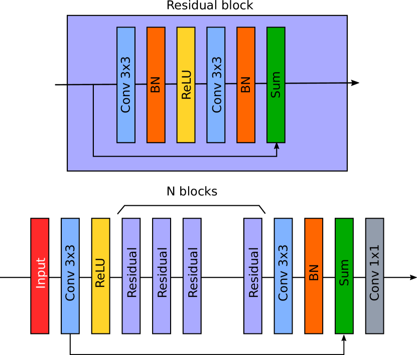
Figure 1: Upper panel: residual block. Lower panel: full architecture of the neural network, made of the concatenation of many residual blocks and a skip connection from the input to the output. We choose $N=20$ for DeepVel.

In this paper we consider the problem of inferring the horizontal velocity field in the solar surface from two consecutive continuum images. The case of only two images represents the worst case scenario and we could have used more frames for the prediction. However, according to the results we present in the following, we consider that two frames gives surprisingly good results. The end-to-end solution given in this paper, that we term DeepVel, is a deep neural network whose topology is described in the following and is trained using velocities extracted from MHD simulations. The network assumes as input two continuum images of size $\mathrm{N}_{x}\times\mathrm{N}_{y}$, separated by 30 s. The outputs are maps of $v_{x}$ and $v_{y}$ at all locations and at three heights in the atmosphere, corresponding to $\tau_{500}=1,0.1,0.01$, with $\tau_{500}$ being the optical depth at 500 nm. Only the results at $\tau_{500}=1$ can be compared with other algorithms like LCT.

2.1 Deep Neural Network topology

The deep network that we use has a fully convolutional architecture, that applies a series of convolutions with several small kernels (to be inferred during the training) to the input of every layer. The architecture is graphically represented in Fig. 1. Each colored rectangle in the figure represents a different layer, that we describe in the following:

• Input (red): this layer represents the two input images of size $\mathrm{N}_{x}\times\mathrm{N}_{y}$. Consequently, this layer represents tensors of size $2\times\mathrm{N}_{x}\times\mathrm{N}_{y}$.

• Conv 3$\times$3 (blue): these layers represent three-dimensional convolutions with a set of 64 kernels (channels) of size $N_{\mathrm{input}}\times 3\times 3$. We keep the number of kernels and their size fixed because they give very good results, with the advantage that convolutions with $3\times 3$ kernels can be made very fast in GPUs. The output tensors of these layers have size $64\times N_{x}\times N_{y}$.

• ReLU (yellow): these layers represent rectified linear units, which apply the following operation to every pixel and channel of the input: $\mathrm{ReLU}(x)=x$ if $x\geq 0$ and zero elsewhere.

• BN (orange): this layer represents batch normalization (Ioffe & Szegedy, 2015), a trick used to increase the convergence speed of the training. It is based on normalizing the input so that it has zero mean and unit variance, which has been verified to greatly accelerate the training.

• Sum (green): this layer describes pixelwise addition between the two inputs.

• Conv 1$\times$1 (grey): this layer defines three-dimensional convolution with six $64\times 1\times 1$ kernels, which is just a very convenient way to collapse the 64 channels of the last Sum layer of the neural network into the six velocities that we want to predict. The output tensor of this layer has size $6\times N_{x}\times N_{y}$.

As seen from the lower panel of Fig. 1, the network is made of the concatenation of N so-called residual blocks (He et al., 2016). We choose $N=20$ for our implementation and did not carry out any hyperparameter optimization, that we leave for the future with the aim of optimizing the network. The internal description of each residual block is displayed in the upper panel of Fig. 1. It is essentially made of two convolution layers, each one followed by batch normalization layers and only the first one containing a ReLU activation. Finally, the input of the block is added pixelwise at the end. The main advantage of the residual blocks is that it accelerates the training thanks to the skip connection between the input and the output. The output of the set of residual blocks is then transferred through an additional convolutional layer with 64 kernels of 3 $\times$ 3 and a batch normalization layer. The output is then obtained after convolution with 6 kernels of size $1\times 1$. The total number of free parameters of the network is $\sim$1.6 $\times$ 10⁶.

2.2 Training data and training process

The network is trained using synthetic continuum images from the magneto-convection simulations described by Stein & Nordlund (2012) and Stein (2012). This simulation box is $\sim$48 Mm wide in both directions and 20.5 Mm deep, extending from the temperature minimum down to 20 Mm below the visible surface. The simulated solar time spans more than an hour in steps of 30 s. The horizontal resolution turns out to be 48 km, with a total size of 1008 $\times$ 1008 pixels. This simulation displays an appropriate balance between the amount of solar surface simulated and the horizontal resolution. The mhd48-1 snapshots that we use are obtained by advecting a uniform field at the bottom boundary. This field is increased until it reaches 1 kG at the bottom boundary and then kept constant.

The synthetic images are then treated to simulate a real observation. We choose the Imaging Magnetograph eXperiment (IMaX; Martínez Pillet et al., 2011) on board the Sunrise balloon borne observatory (Solanki et al., 2010; Barthol et al., 2011) as a target. Sunrise has a telescope of 1 m diameter and the images that IMaX provides have a spatial sampling of 39.9 km. It is interesting to note that the spatial sampling of the simulated images used in the training and those of IMaX do not exactly coincide (48 km vs. 39.9 km). However, we demonstrate later than an appropriately trained network will generalize correctly independently of the size of the structures.

Given that Sunrise was a balloon mission that observed at a height of $\sim$ 40 km above the Earth surface, the observations are barely affected by the atmosphere. One of the reasons to choose IMaX in our tests is that the instrument has provided long time series of very high-quality diffraction-limited images in both flights (e.g., Lagg et al., 2010; Martínez González et al., 2011; Solanki et al., 2017), which have been used often for LCT studies (e.g., Bonet et al., 2010; Yelles Chaouche et al., 2011; Requerey et al., 2014, 2017). We simulate the effect of IMaX following the approach of Asensio Ramos et al. (2012), which is based on the detailed analysis of Vargas Domínguez (2009). We consider telescope aberrations up to 45 Zernike modes. The amplitudes are considered to be normally distributed with diagonal covariance and a total rms wavefront error (WFE) amounting to $\lambda/9$. These telescope aberrations can be considered to be constant during an observation, so we keep them fixed. The remaining atmosphere is accounted for by considering a wavefront with turbulent Kolmogorov statistics (Noll, 1976) with a rms WFE of $\lambda/9$. Although these perturbations are very specific for Sunrise/IMaX, we think that the neural network trained with these images can be safely applied (or perhaps easily re-trained for different instrumental configurations).

From the available three-dimensional volume of 1008 $\times$ 1008 continuum images for all timesteps, we randomly extract two patches of 50$\times$50 pixels in the same spatial position and separated by 30 s in time. A total of 30000 such pairs are randomly selected as input for the training. The outputs are the six 50 $\times$ 50 images containing $v_{x}$ and $v_{y}$ at $\tau_{500}=1,0.1$ and 0.01, respectively, for each timestep. We also generate another set of 1000 samples using the same strategy, which is used as a validation set to avoid overfitting. These are used during training to check that the deep network generalizes correctly and is not memorizing the training set.

The neural network has been developed using the Keras Python library, with the Tensorflow backend for the computations. All the training is compiled by Tensorflow to be run in the NVIDIA Tesla K40 and Titan X GPUs. The training is carried out by minimizing the squared difference between the output of the network and the velocities in the training set. It is known that optimizing the $\ell_{2}$ norm of the difference might lead to too smooth predictions, which is not appropriate for typical uses of deep networks for machine vision in natural images. In the last few years, improvements in this direction have been performed using a second deep network that is used to measure the quality of the prediction. Both networks are trained as a generative adversarial network (GAN; Goodfellow et al., 2014), which results in impressive results (Ledig et al., 2016). We know from the simulations that the horizontal velocity fields are relatively smooth, so we stick with the simpler $\ell_{2}$ norm for our case. We leave the analysis of using GANs for the training for the future.

All inputs are normalized to the median intensity of the quiet Sun (which also needs to be done once the network is applied to real observations) and velocities are normalized to the interval $[0,1]$ using the minimum and maximum velocities in the training set. The optimization is done with the Adam stochastic first-order gradient-based optimization algorithm (Kingma & Ba, 2014) with a learning rate $\epsilon=10^{-4}$. As in any stochastic optimization method, the gradient is estimated from subsets of the input samples, also known as batches. We use batches of 32 samples and train the network for 30 epochs, where an epoch is finished once all training samples have been used. Therefore, the number of iterations is then 900000.

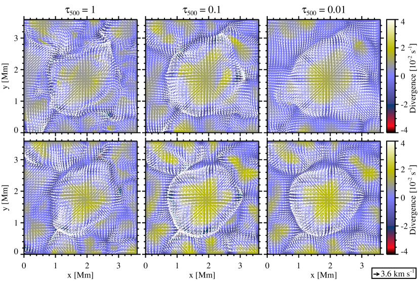
Figure 2: Instantaneous horizontal velocity field (white arrows) and divergence maps (background images) at three heights in the atmosphere, corresponding to $\tau_{500}=1,0.1,0.01$, for MANCHA (upper row) and DeepVel (bottom row) velocities.

2.3 Validation

In absence of a technique similar to DeepVel that can be applied to observations, we validate the method using 3D magneto-convection simulations carried out with the MANCHA code (Felipe et al., 2010; Khomenko et al., 2017). The extent of the simulation domain is 24 Mm $\times$ 24 Mm in the horizontal plane and 1.4 Mm vertically, with 1152 grid cells in each horizontal direction and 102 uniformly spaced grid points in the vertical direction. The domain is open for the mass flows at the bottom boundary and closed at the top. The radiative transfer losses are computed assuming local thermodynamical equilibrium with precomputed opacities. The magnetic field is initiated through the Biermann battery and amplified by the local dynamo (similarly to Vögler & Schüssler, 2007). The snapshots used in this study were taken when the total magnetic field reached 10 G at the unit optical depth. The synthetic continuum maps are degraded so that the pixel size is equivalent to those of the training set. We use two consecutive continuum maps to infer the horizontal velocity field and compare it with the ones extracted from the simulations. The upper panels of Fig. 2 display the velocity fields of the simulations at three different optical heights in the atmosphere. The underlying map is the divergence of the horizontal field, which is computed as $\nabla\,\mathbf{v}=\partial v_{x}/\partial x+\partial v_{y}/\partial y$ for $\mathbf{v}=(v_{x},v_{y})$. Note that positive values indicate diverging flows, while negative values point to converging flows. The lower panels display the results of DeepVel, which very nicely reproduce the results from the simulation, specially for $\tau_{500}=1,0.1$. The results for $\tau_{500}=0.01$ are slightly less similar although the general appearance is still valuable. Figure 2 only shows a small field of view (FOV), but similar results are found for the rest of the simulated field. Specifically, the velocity field vectors of the whole simulated FOV have a Pearson linear correlation coefficient of 0.82, 0.85, and 0.76 for $\tau_{500}=1,$ 0.1, and 0.01, respectively. Additionally, $v_{x}$ displays correlation coefficients of 0.82, 0.84, and 0.75 for the same values of $\tau_{500}$, while the figures turn out to be 0.83, 0.86, and 0.78 for $v_{y}$ for the same $\tau_{500}$ heights. We consider that this experiment validates DeepVel.

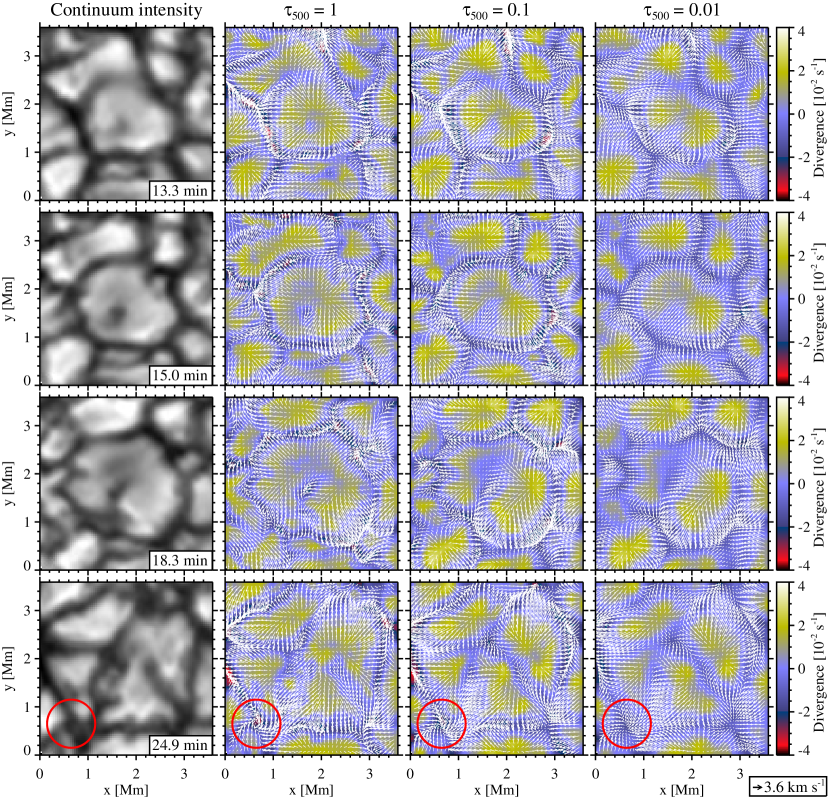
Figure 3: Evolution of granules as seen in close-ups of continuum intensity maps (left column) and the instantaneous horizontal velocity field (white arrows) and divergence maps (background images) at three heights in the atmosphere (right columns), corresponding to $\tau_{500}=1,0.1,0.01$. The area is located within the black solid rectangle in Fig. 4(a). Red circles (with a radius of 0.5 Mm) in the bottom row indicate the location of a small-scale vortex flow. Elapsed time is given in the bottom-right corner of each continuum image. The whole evolution is presented in a movie provided as online material. The arrow at the lower right corner can be used to visually estimate the amplitude of the velocity field. The whole evolution is presented in a movie provided as online material.

3 Results

Once the network is trained, we apply it to real IMaX observations from the first Sunrise flight. The observational data were obtained on 2009 June 9 from 01:30:54 to 02:02:29 UT, in a quiet-Sun region close to disk center. The 31.6 min length dataset has a temporal cadence of 33.25 s. We point out that the temporal cadence is larger than the one used in the training, so that the network might slightly overestimate the velocities. We also note that the spatial resolution of the observations is also slightly better than those of the simulations, but we do not expect large effects. Even though the training was done with images of size 50 $\times$ 50, given the fully convolutional character of the network, we apply it seamlessly to the full FOV of the instrument, that amounts to 736 $\times$ 736 pixels (29.3 $\times$ 29.3 Mm²). The computing time is $\sim$2 s per image using a Titan X GPU, and an order of magnitude larger if the computation is done in a CPU.

3.1 Inferred velocity fields

In Fig. 3 and the movie in the online material, we display the inferred horizontal velocity field for a small portion of the FOV at four different time steps. The first column shows the continuum image, while the rest of columns display the divergence of the horizontal velocity field at the three different heights in the atmosphere, together with the instantaneous vector field. Note that the results displayed in Fig. 3 are impossible to be obtained using LCT due to the somehow large spatial and temporal smearing windows that need to be used to increase the correlation and produce robust results.

In general, velocities in lower layers tend to be larger in absolute value and also with larger spatial complexity. Although horizontal diverging flows are similar at the three heights considered, stronger converging flows are seen in intergranular lanes in deeper layers. Additionally, the horizontal size of these zones of converging flows is much smaller in deep layers.

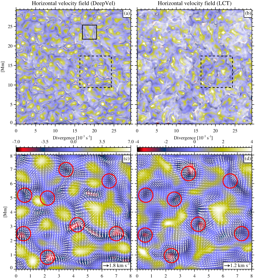
Figure 4: Average horizontal velocity field (white arrows) and divergence maps (background images) for the FOV of IMaX computed by DeepVel (a) and LCT (b), respectively. The black solid box marks the region analyzed in Fig. 3. Close-ups of the black dashed rectangles are shown in panels (c) and (d) for DeepVel and LCT, respectively. Red circles represent the locations of converging flows.

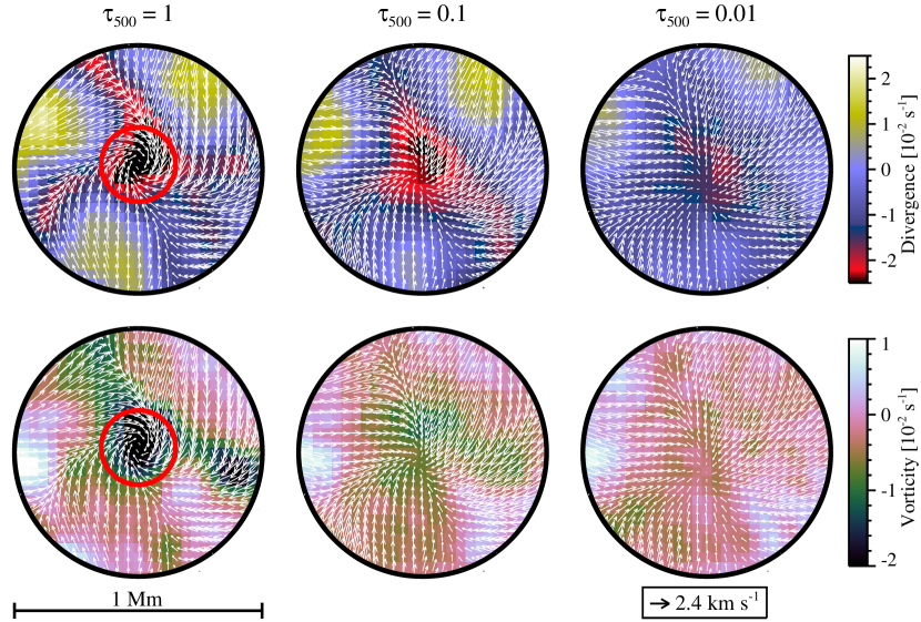
Figure 5: Close-up of the small-scale vortex flow shown in Fig. 3 by red circles. The upper panels show the divergence of the horizontal velocity field at the three selected heights, while the lower panels display the vertical vorticity. Red circles (with a radius of 150 km) show the size of the small-scale vortex flow.

We find very interesting the behavior observed in some granules at $t=15$ min, like the one at positions $(x,y)=(0.8,2.6)$ Mm. This granule appear to be formed by the aggregation of two or more smaller portions. The continuum image of the granule shows a slightly dark lane separating bright regions. This structure is also clearly seen in the velocity field at $\tau_{500}=0.1$ and $\tau_{500}=0.01$, while it disappears for deeper layers. It looks like these dark lanes in the middle of granules are a consequence of a converging flow in upper layers that does not reach very deep. Interestingly, the velocity fields before ($t=13.3$ min) and after ($t=18.3$ min) help us understand what is happening. We are witnessing a fragmenting granule that is being divided into two by a converging velocity field taking place at higher layers, which later propagates towards lower layers. Note that at $t=13.3$ min, the division is barely visible in the intensity image, but it is already present at $\tau_{500}=0.01$. Finally, at $t=18.3$ min, the granule is divided in two parts, with a clear intergranule between them. Our observations seem to be compatible with the buoyancy-braking mechanism (Massaguer & Zahn, 1980; Ploner et al., 1999). In this model, the gas above large granules reduce their upward velocity because of the increase in the mass in upper layers. It looses buoyancy and catastrophically collapses forming a dark lane if energy losses cannot be compensated. According to our observations, it also develops strong converging velocity flows when eventually forming a new intergranular lane. The fact that DeepVel shows this behavior means that this mechanism has to be the predominant one in the simulations and that the behavior in upper layers is connected to what is going on at lower layers.

Other instances of fragmenting granules and appearance of dark structures inside bright granules can be seen in the observations. They all appear to share a similar behavior, except for the specific details. For instance, the dark spot at $(x,y)=(1.6,1.4)$ Mm at $t=15$ min seems to reach lower layers slightly faster than the previous example.

3.2 Comparison with LCT

In order to test the performance of DeepVel, we compare it with the well known LCT algorithm. The LCT technique recovers horizontal proper motions by tracking intensity features in continuum images. We use a Gaussian tracking window with an FWHM = 600 km and then average the cross-correlation function over 30 min. We confront this velocity field with that obtained by DeepVel at $\tau_{500}=1$, temporally averaged over 30 min. In addition, the vector field is spatially averaged with the LCT tracking window size. The top panels of Fig. 4 show the horizontal velocity arrows and the corresponding divergence maps obtained by DeepVel (Fig. 4a) and LCT (Fig. 4b) for the whole FOV of IMaX. We find that the DeepVel velocities are $1.15$ times larger in magnitude than the LCT ones, which almost perfectly coincides with the overestimation expected because measurements in IMaX are taken every 33.25 s, instead of the 30 s used in the training (the correction factor would be ($\times$1.11). The velocity fields have Pearson linear correlation coefficients of 0.81 and 0.84 for $v_{x}$ and $v_{y}$, respectively, while it goes down to 0.8 for the whole velocity vector. Additionally, the correlation coefficient for the divergence is $0.71$.

This correlation is already evident from the visual inspection of the flow and divergence maps. The bottom panels of Fig. 4 display an enlarged view of a smaller region, marked by a black dashed rectangle in the upper panels. Even though there exist some morphological differences, both maps show the same flow features. In particular, they display an equivalent mesogranular pattern, which is revealed through positive divergence structures on scales between granulation and supergranulation. Such a cellular pattern is commonly found in both observations and hydrodynamical simulations when the LCT technique is applied to intensity images (Simon et al., 1988; Muller et al., 1992; Roudier et al., 1998; Matloch et al., 2010; Yelles Chaouche et al., 2011; Requerey et al., 2017). At the junction of mesogranular cells, smaller structures such as converging flows (Bonet et al., 2010; Vargas Domínguez et al., 2011; Requerey et al., 2017) are also observed. The locations of the convergence centers are marked by red circles in Fig. 4(c) and (d). Despite their small size, they are equally retrieved in both velocity fields.

The time-averaging increases the correlation between the simulated plasma velocities and the LCT ones (Rieutord et al., 2001; Matloch et al., 2010). The same applies for the correlation between the smoothed DeepVel velocities and the LCT flows. Specifically, we get correlation coefficients of 0.71, 0.75, 0.79, and 0.80 for averaging times of 5, 10, 20, and 30 min, respectively. This results from the fact that the DeepVel velocities are a reliable representation of the instantaneous horizontal flow fields, while the LCT velocities are only comparable to plasma velocities typically at time scales longer than the average granule lifetime.

3.3 Small-scale vortex flow

Small-scale vortex flows have been first detected as swirling motions of bright points (Bonet et al., 2008), and later through LCT (Bonet et al., 2010; Vargas Domínguez et al., 2011; Requerey et al., 2017). They have a diameter of $\sim$ 1 Mm (Bonet et al., 2008, 2010; Vargas Domínguez et al., 2011), their lifetime varies from 5 to 20 min (Bonet et al., 2008, 2010), and they appear located at mesogranular junctions (Requerey et al., 2017). The spatial distribution and size of such vortices is shown by red circles in Fig. 4(d). The temporal and spatial scales are larger than those expected from simulations, where the vortices have lifetimes of only a few minutes ($\sim$ 3.5 min) and diameters of $\sim$ 100 km (Moll et al., 2011). This differences are likely due to the smoothing produced by the time and spatial average of the LCT technique.

Figure 5 shows the velocity fields for a close-up of the vortex flow marked in Fig. 3 by red circles. The underlying maps in the upper panels show the divergence, while the lower panels display the vertical vorticity of the horizontal velocity field, defined as $(\nabla\times\mathbf{v})_{z}=\partial v_{y}/\partial x-\partial v_{x}/\partial y$. The vortex has a very small size, surely smaller than 300 km in diameter (see red circle in Fig. 5), and lasts for a very short time, in the range 30-60 s, because it is only clearly visible in one time step, and can be guessed in the previous and next frames.

The vortex flow has a central zone with a very strong negative divergence at $\tau_{500}=1$, reaching values up to $-0.03$ s^-1, which are more than an order of magnitude larger than the median value found by Requerey et al. (2017) as a consequence of the much smaller size. The same behavior is seen in the vorticity, with values that also reach $-0.03$ s^-1 at $\tau_{500}=1$, negative meaning clockwise rotation. This value of vorticity is an order of magnitude larger than that detected with LCT (Bonet et al., 2010; Vargas Domínguez et al., 2011; Requerey et al., 2017), but comparable to that found in simulations (e.g., Kitiashvili et al., 2011).

Interestingly, the DeepVel results show a different picture of the vortex flow at higher layers. First, material is still strongly advected towards the center of the vortex, with divergences that are still of the order of $-0.02$ s^-1, while the vorticity becomes much smaller in higher layers. This behavior resembles that of the “bathtub effect” (Nordlund, 1985), in which the circular velocity is amplified as the plasma contracts with depth.

4 Conclusions

We have developed DeepVel, an end-to-end approach for the estimation of instantaneous and per-pixel horizontal velocity fields based on a deep network. The network is fully convolutional, so that it can be applied to input images of arbitrary size, providing outputs of exactly the same size. In addition, it is very fast, has no parameters to be tuned and is available to the community as open source. Concerning speed, we note that it can be improved with some architectural changes, but we think that it is already fast enough for our standards.

We have checked that the spatially and temporally averaged horizontal velocity field provided by the network is very similar to that obtained with LCT. However, the power of DeepVel is that this same information can also be obtained instantaneously, contrary to LCT. Additionally, we provide the velocity field at three different heights in the atmosphere, something that might look counterintuitive at a first look. It is clear from the results presented here (both from simulations and observations) that the network is able to correctly generalize and is not overfitting.

Similar to this application, we expect deep learning to be increasingly applied to Solar Physics as more high-quality data is obtained and needs to be analyzed. An incomplete list of possible potential applications in which we are already working on would include fast image deconvolution, fast 2D and 3D spectropolarimetric inversions, fast control of adaptive optics, etc.