$\mathcal{PT}$-symmetric wave guide system with evidence of a third-order exceptional point

Abstract

An experimental setup of three coupled $\mathcal{PT}$-symmetric wave guides showing the characteristics of a third-order exceptional point (EP3) has been investigated in an idealized model of three delta-functions wave guides in W. D. Heiss and G. Wunner, J. Phys. A 49, 495303 (2016). Here we extend these investigations to realistic, extended wave guide systems. We place major focus on the strong parameter sensitivity rendering the discovery of an EP3 a challenging task. We also investigate the vicinity of the EP3 for further branch points of either cubic or square root type behavior.

I Introduction

The term “exceptional point” (EP) originates from a purely mathematical context and describes branch point singularities in the spectrum of parameter-dependent linear operators Kato (1966). However, by now there is an overwhelming interest in physics Heiss (2012) on this topic both theoretically (see e.g. Heiss and Sannino (1990); Heiss (2000); Hernández et al. (2006); Lefebvre et al. (2009); Cartarius et al. (2009); Cartarius and Moiseyev (2011); Gutöhrlein et al. (2013); Wiersig (2014); Schwarz et al. (2015); Menke et al. (2016)) and experimentally (see, e.g. Philipp et al. (2000); Dembowski et al. (2003); Dietz et al. (2007); Stehmann et al. (2004); Lawrence et al. (2014); Gao et al. (2015); Doppler et al. (2016); Xu et al. (2016)). In general EPs are positions in some parameter space, at which two (EP2) or even $N>2$ (EP$N$) eigenvalues, as well as the corresponding eigenvectors, coalesce in a branch point singularity. These points can be found in the vicinity of level repulsion if one external system parameter is analytically continued into the complex plane Heiss (1999). This renders the underlying Hamiltonian describing the physics of the system to be no longer Hermitian Morse and Feshbach (1953). In fact, exceptional points can only occur for non-Hermitian Hamiltonians. The manifestation of exceptional points is not only restricted to quantum systems. For non-Hermitian systems, they also occur in classical mechanics Heiss and Wunner (2015) as well as in optics Lee et al. (2009); Longhi (2010); Guo et al. (2009); Chong et al. (2011); Ge and Stone (2014); Chang et al. (2014); Feng et al. (2014); Hodaei et al. (2014) and microwave cavities Dembowski et al. (2001). In order to obtain a unitary theory the non-Hermiticity requires the definition of a new inner product – the bi-orthogonal product or c-product Brody (2014); Moiseyev (2011). At the exceptional points the corresponding Hilbert space becomes defective in that the number of eigenvectors is reduced as a consequence of the coalescence.

EPs show more characteristic properties than those mentioned above: In their simplest manifestation, i.e., for an EP2, the two eigenvalues can be mathematically described by two branches of the same analytic function, thus showing typical square root behavior. This means, if one encircles the EP2 along a closed loop in the physical parameter space the corresponding eigenvalues forming an EP2 permute. Exceptional points of higher order, e.g., third-order exceptional points, show cubic root behavior, i.e., one typically observes a threefold state exchange performing a closed loop around the EP3. Moreover, since also the eigenvectors coalesce at the exceptional point – forming a self-orthogonal state Moiseyev (2011) – the corresponding Hamiltonian in matrix representation is no longer diagonalizable. With a similarity transformation, however, one can transform it to a Jordan normal form. There an exceptional point of order $N$ is represented in terms of an $N$-dimensional Jordan block Günther et al. (2007).

Exceptional points appear in particular in $\mathcal{PT}$-symmetric systems, i.e., systems which are symmetric under the combined action of the parity operator $\mathcal{P}$ and the time reversal operator $\mathcal{T}$. Bender and Boettcher Bender and Boettcher (1998) demonstrated that $\mathcal{PT}$-symmetric non-Hermitian Hamiltonians can possess real eigenvalues. When the real eigenvalues coalesce and turn into complex conjugates the underlying $\mathcal{PT}$ symmetry is broken. The parameter set at which the symmetry is broken marks the position of an exceptional point. As this class of non-Hermitian Hamiltonians is in particular predestined for the occurrence of EPs they have been investigated in a wide range of systems ranging from fundamental questions in quantum mechanics Bender et al. (1999); Znojil (1999); Jones and Moreira (2010), quantum field theories Bender et al. (2012); Mannheim (2013) to Bose-Einstein condensates in the mean-field approximation Graefe (2012); Dast et al. (2013); Abt et al. (2015); Gutöhrlein et al. (2015) and many-particle descriptions Graefe et al. (2008a); Dast et al. (2016), where complex potentials model the gain and loss of particles Kreibich et al. (2016); Dast et al. (2014). $\mathcal{PT}$ symmetry has also been studied in cavities for electromagnetic waves Bittner et al. (2014); Peng et al. (2014); Bender et al. (2013), optical structures with complex refractive indices Makris et al. (2008); El-Ganainy et al. (2007), and in electronic devices Schindler et al. (2011). Spectral singularities in $\mathcal{PT}$-symmetric potentials Mostafazadeh and Mehri-Dehnavi (2009) turned out to be connected with the amplification of waves Mostafazadeh (2013a) and the lasing threshold Mostafazadeh (2013b).

Klaiman et al. Klaiman et al. (2008) proposed an experimental setup of two coupled $\mathcal{PT}$-symmetric wave guides with complex refractive index for the visualization of second-order branch points. The imaginary parts are interpreted as gain (loss) of the field intensity, e.g., by optical pumping and absorption. Its strength controls the non-Hermiticity. Their investigations showed the coalescence of the system’s eigenmodes, experimentally observable in terms of an increasing beat length in the power distribution of the total field. The predictions received convincing experimental confirmation 2010 by Rüter et al. Rüter et al. (2010).

While the physics of EP2s is well investigated, lesser attention has hitherto been paid to exceptional points of higher order Graefe et al. (2008b); Heiss (2008); Demange and Graefe (2012); Heiss and Wunner (2016); Ge (2015); Ding et al. (2016); Lin et al. (2016); Jing et al. (2016). New effects were shown in the different theoretical models of higher order EPs. In Heiss (2008) a chiral behavior of the eigenfunctions in the neighborhood of three coalescing eigenfunctions was reported. In Demange and Graefe (2012) it was shown that encircling an EP3 does not necessarily show the typical third-root behavior. In this context a possible experiment made up of three coupled wave guides was proposed in terms of an abstract mathematical matrix model. Here our work sets in. Encouraged by the experimental confirmation of the wave guide system investigated in Klaiman et al. (2008) we extend this model by placing a third wave guide between those with gain and loss but with only a real part of the refractive index that may be different from that of the outer ones. We show that this model gives rise to a third-order exceptional point by solving the whole system semi-analytically. We work out explicitly the appearance of further EP2s or EP3s in the vicinity of the original EP3 as was discussed qualitatively in Heiss (2008); Demange and Graefe (2012).

The paper is organized as follows. Sec. II introduces the system including the corresponding equations. These are solved in Sec. III, where we demonstrate the manifestation of the EP3, its verification as well as the total power distribution. In Sec. IV we explicitly demonstrate the additional EP2s and EP3s in the space of the system’s physical parameters. In Sec. V we summarize the crucial points and give an outlook to ongoing work.

II The $\mathcal{PT}$-symmetric optical wave guide system

We model a $\mathcal{PT}$-symmetric wave guide system for the experimental observation of a third-order branch point with three coupled planar wave guides on a background material with refractive index $n_{0}=3.3$, as depicted in Fig. 1.

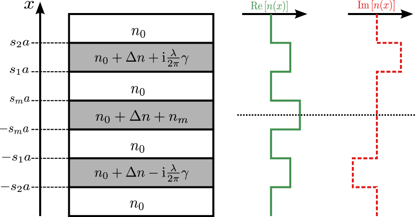
Figure 1: $\mathcal{PT}$-symmetric directional coupling. The structure consists of three coupled slab wave guides on a background material with index $n_{0}=3.3$. The right hand side displays the real and imaginary part of the refractive index, which only vary in $x$ direction. Using the dimensionless parameters $s_{m}$ and $s_{1,2}$ the wave guides’ width as well as the separation between them is adjusted. Here a value of $a=$2.5\text{\,}\mathrm{\SIUnitSymbolMicro m}$$ is chosen. Also note that we allow for a larger real index difference between the middle wave guide and the background material as compared to the outer ones by adding an additional term $n_{m}$ to the fixed one $\Delta n=1.3\times 10^{-3}$. The imaginary part of the index can be controlled by the gain-loss coefficient $\gamma$ with the vacuum wavelength taken to be $\lambda=$1.55\text{\,}\mathrm{\SIUnitSymbolMicro m}$$.

We assume the refractive index to vary only in $x$ direction with a symmetric index guiding profile and an antisymmetric gain-loss profile, i.e., $n(x)=n^{*}(-x)$ to sustain $\mathcal{PT}$ symmetry. For three wave guides we basically follow the approach used in Klaiman et al. (2008) for two wave guides, but in addition we allow for more flexibility of the wave guides’ parameters. Their width and the separation between them can be varied with dimensionless scaling factors $s_{m}$ and $s_{1,2}$ in order to define distances via the constant length scale $a=$2.5\text{\,}\mathrm{\SIUnitSymbolMicro m}$$ (cf. Fig. 1). Moreover we chose $\Delta n=1.3\times 10^{-3}$ and allow for a different real index difference between the middle wave guide and the background material as compared to the outer ones by adding an additional term $n_{m}$. The imaginary part of the refractive index can be controlled by the non-Hermiticity parameter $\gamma$ with the vacuum wavelength taken to be $\lambda=$1.55\text{\,}\mathrm{\SIUnitSymbolMicro m}$$. A realization of the system studied in this work is possible with GaAs or ZnSiAs₂ as guiding material. The variations of the refractive index are possible with a carrier-induced change Dutta et al. (1992), electric field induced changes Susa (1995), or femtosecond-scale switching Ganikhanov et al. (1999).

The direction of propagation in the wave guides is taken to be the $z$ axis, such that the wave equation for the transverse-electric modes reads

$$\left(\frac{\partial^{2}}{\partial x^{2}}+k^{2}n(x)^{2}\right)\mathcal{E}_{y}(x)=\beta^{2}\mathcal{E}_{y}(x)\,,$$ (1)

where the $y$ component of the electric field is given by $E_{y}(x,z,t)=\mathcal{E}_{y}(x)\mathrm{e}^{\mathrm{i}(\omega t-\beta z)},$ with $k=2\pi/\lambda$ and the propagation constant $\beta$. Obviously Eq. (1) is formally equivalent to a one-dimensional stationary Schrödinger equation with potential $V(x)=-\frac{1}{2}k^{2}n(x)^{2}$ and energy eigenvalue $E=-\frac{1}{2}\beta^{2}\,.$ Thus the quantum mechanical analogue of the arrangement shown in Fig. 1 is a configuration of three finite potential wells with gain or loss in the two outer wells.

Because of the underlying $\mathcal{PT}$ symmetry there is some range of $\gamma$, for which $\beta$ is purely real. The point at which all three modes break this symmetry simultaneously and become complex, is associated with an EP3. The challenging part in a numerical simulation, as well as in an experiment, is to find the correct values for the system parameters $(\beta,\gamma,s_{m},s_{1},s_{2},n_{m},\Delta n)$ to determine this point.

III Solution of the full wave guide system

III.1 Semi-analytical approach and method for finding an EP3

The stationary modes can be taken to be

$$\tilde{\mathcal{E}}_{y}(x) =\begin{cases}A_{1}\mathrm{e}^{\kappa x}+A_{2}\mathrm{e}^{-\kappa x}&:\;-\infty<x<-s_{2}a\\ B\mathrm{e}^{\mathrm{i}q_{l}x}+C\mathrm{e}^{-\mathrm{i}q_{l}x}&:\;-s_{2}a\leq x\leq-s_{1}a\\ D_{1}\mathrm{e}^{\kappa x}+D_{2}\mathrm{e}^{-\kappa x}&:\;-s_{1}a<x<-s_{m}a\\ F\mathrm{e}^{\mathrm{i}q_{m}x}+G\mathrm{e}^{-\mathrm{i}q_{m}x}&:\;-s_{m}a\leq x\leq s_{m}a\\ H_{1}\mathrm{e}^{\kappa x}+H_{2}\mathrm{e}^{-\kappa x}&:\;s_{m}a<x<s_{1}a\\ K\mathrm{e}^{\mathrm{i}q_{r}x}+L\mathrm{e}^{-\mathrm{i}q_{r}x}&:\;s_{1}a\leq x\leq s_{2}a\\ M_{1}\mathrm{e}^{-\kappa x}+M_{2}\mathrm{e}^{\kappa x}&:\;s_{2}a<x<\infty\end{cases}$$ (2)

with the parameters

$$\kappa^{2} =\beta^{2}-k^{2}n_{0}^{2}\,,$$ (3a)

$$q_{l}^{2} =-\beta^{2}+k^{2}\left(n_{0}+\Delta n-\mathrm{i}\frac{\lambda}{2\pi}\gamma\right)^{2}\,,$$ (3b)

$$q_{m}^{2} =-\beta^{2}+k^{2}\left(n_{0}+\Delta n+n_{m}\right)^{2}\,,$$ (3c)

$$q_{r}^{2} =-\beta^{2}+k^{2}\left(n_{0}+\Delta n+\mathrm{i}\frac{\lambda}{2\pi}\gamma\right)^{2}\,.$$ (3d)

Similar to the procedure in Mostafazadeh and Mehri-Dehnavi (2009) the continuity conditions at the potential barriers can be combined in a transition matrix $\mathbf{T}\in\mathbb{C}^{2\times 2}$ relating the coefficients of the two outermost parts of the system Yeh (1988). Thus the whole physics of the system is incorporated in this matrix. To obtain physical meaningful solutions out of Eq. (2) the condition

$$A_{2}=M_{2}=0$$ (4)

has to be fulfilled. Then the relation just mentioned between the system’s left- and right-hand sides reads

$$\begin{pmatrix}A_{1}\\ 0\end{pmatrix} =\mathbf{T}\cdot\begin{pmatrix}M_{1}\\ 0\end{pmatrix}$$

$$=\begin{pmatrix}T_{11}&T_{12}\\ T_{21}&T_{22}\end{pmatrix}\cdot\begin{pmatrix}M_{1}\\ 0\end{pmatrix}\,,$$ (5)

which is only true for

$$T_{21}\left(n_{0},\lambda,a;\beta,\gamma,s_{m},s_{1},s_{2},n_{m},\Delta n\right)=0\,.$$ (6)

This is the condition from which the complex propagation constants $\beta$ are found by a two-dimensional root search. To enforce the coalescence into an EP3 the additional conditions

$$T_{21}=\frac{\partial T_{21}}{\partial\beta}=\frac{\partial^{2}T_{21}}{\partial\beta^{2}}=0\,$$ (7)

have to be obeyed. These additional equations enforce the zero to be threefold, which is necessary for an EP3. With these equations we are able to determine $\beta$ as well as the system parameters $\gamma,s_{m},s_{1}$ and $n_{m}$ by a six-dimensional root search while we fix $s_{2}$ and $\Delta n$.

III.2 Manifestation and verification of an EP3

Using the method just described an EP3 is found on the real $\beta$ axis at

$$\beta_{\mathrm{EP3}} =13.37936893005811\,,$$ (8a)

$$\gamma_{\mathrm{EP3}} =0.2568441576999367\,,$$ (8b)

$$s_{m}^{\mathrm{EP3}} =1.006301260784219\,,$$ (8c)

$$s_{1}^{\mathrm{EP3}} =8.983140907622532\,,$$ (8d)

$$n_{m}^{\mathrm{EP3}} =1.873188792979378\times 10^{-6}\,,$$ (8e)

with the fixed parameters

$$s_{2}^{\mathrm{EP3}} =11.0\,\quad\text{and}\quad\Delta n =1.3\times 10^{-3}\,.$$ (9)

The propagation constants of the three guided modes in the wave guides are plotted in Fig. 2 as a function of the non-Hermiticity parameter, with the other system parameters set to the values according to Eqs. (8) and (9). Obviously the first excited state’s propagation constant is virtually independent of the gain-loss parameter gamma. This behavior seems to be typical for a setup of three coupled wave guides since it also appears for the idealized delta-functions model Heiss and Wunner (2016). It also appears for special distributions of the gain and loss in flat band systems Ge (2015); Ge and Qi (2017).

It can be seen that increasing $\gamma$ leads to an (inverse) bifurcation structure of the propagation constants. It is the movement of the two outer eigenvalues towards each other with an essentially constant middle value into the third-order exceptional point at $\gamma_{\mathrm{EP3}}$. Beyond this point (gray area) the propagation constants become complex. Thus we confirm the findings for two coupled $\mathcal{PT}$-symmetric wave guides in Klaiman et al. (2008), i.e., one may study the exceptional point by varying only a single parameter. This is in contrast to the idealized delta-functions model Heiss and Wunner (2016), in which two parameters have to be varied in steps to reach the EP3 starting from $\gamma=0$.

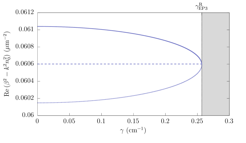
Figure 2: Propagation constants of the three guided modes of the wave guide system depicted in Fig. 1 as a function of the non-Hermiticity parameter $\gamma$. As $\gamma$ is increased the outer eigenvalues approach each other while the middle mode is mostly unaffected by this variation. For $\gamma_{\mathrm{EP3}}\approx 0.2568\,\mathrm{cm}^{-1}$ the eigenmodes coalesce in a third-order exceptional point. Beyond this branch point (gray area) the propagation constants become complex.

For this, however, it is necessary to adjust the system parameters exactly according to Eqs. (8) and (9) to end up in an EP3 within a numerical simulation. Deviations from these values will lead to a coalescence of merely two modes. At this point we encounter the perhaps most difficult part in an experimental realization – the exceeding sensitivity to changes in the setup of the system parameters.

We verify the expected properties of the EP3 by encircling the branch point. We introduce asymmetry parameters breaking the underlying $\mathcal{PT}$ symmetry by adding $a=a_{\mathrm{r}}+\mathrm{i}a_{\mathrm{i}}$ to the refractive index of the left wave guide and $b=b_{\mathrm{r}}+\mathrm{i}b_{\mathrm{i}}$ to the right one, which changes the parameters $q_{l}$ and $q_{r}$ from Eqs. (3b) and (3d), viz.

$$\tilde{q}_{l}^{2} =-\beta^{2}+k^{2}\Bigl{[}n_{0}+\Delta n+{a_{\mathrm{r}}}-\mathrm{i}\Bigl{(}\frac{\lambda}{2\pi}\gamma+{a_{\mathrm{i}}}\Bigr{)}\Bigr{]}^{2}\,,$$ (10a)

$$\tilde{q}_{r}^{2} =-\beta^{2}+k^{2}\Bigl{[}n_{0}+\Delta n+{b_{\mathrm{r}}}+\mathrm{i}\Bigl{(}\frac{\lambda}{2\pi}\gamma+{b_{\mathrm{i}}}\Bigr{)}\Bigr{]}^{2}\,.$$ (10b)

We break the $\mathcal{PT}$ symmetry in either the real or the imaginary part of the refractive index. We perform the loop in the space of this asymmetry and the distance between the wave guides. The distance can be varied with $s_{m}$ whence the loop can be parametrized as

$$\left(\begin{array}[]{c}s_{m}\\ a_{\mathrm{r}}\end{array}\right) =\left(\begin{array}[]{c}s_{m}^{\mathrm{EP3}}+\left(1-s_{m}^{\mathrm{EP3}}\right)\cos\varphi\\ 10^{-6}\sin\varphi\end{array}\right)$$ (15)

with $\varphi\in\left[0,2\pi\right]$ for an asymmetry in the real part as only the refractive index of the left wave guide is varied ($b_{\mathrm{r}}=a_{\mathrm{i}}=b_{\mathrm{i}}=0$). A similar parametrization can be used for an asymmetric variation of the imaginary part, i.e., $a_{\mathrm{i}}=-b_{\mathrm{i}}$. Both situations are depicted in Fig. 3.

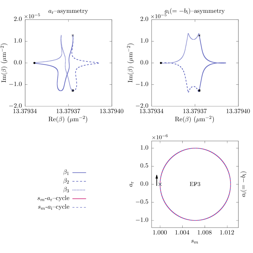
Figure 3: Verification of the EP3 in Fig. 2 by encircling it in the space of asymmetry parameters (breaking the systems $\mathcal{PT}$ symmetry in either the real or imaginary part of the refractive index) and distance (represented by $s_{m}$). The upper panel shows the characteristic threefold permutation if one encircles the EP3 in the $s_{m}$-$a_{\mathrm{r}}$–space (left) or in the $s_{m}$-$a_{\mathrm{i}}\leavevmode\nobreak\ (=-b_{\mathrm{i}})$–space (right). The starting points of the respective eigenvalues are depicted by specific symbols. They are the end points of the paths of another eigenvalue. Thus, one can see that the disturbed ground state branch (left-most starting point) ends at the starting point of one of the excited states. The path starting there ends at the starting point of the second of the excited states. Finally, the path of the latter ends at the starting point of the disturbed ground state. The corresponding curves shown on the bottom right are parametrized according to Eq. (15), where the loop is performed clockwise for both circles.

The characteristic threefold permutation of the propagation constants becomes obvious in both cases while the circle for the $a_{\mathrm{i}}/-b_{\mathrm{i}}$–asymmetry shows higher symmetry compared to the loop performed in the $s_{m}$-$a_{\mathrm{r}}$–space.

Note that the numerical precision achieved in this work as shown in Eq. (8) is not realizable in an experiment. However, as the EP3 splits into two EP2s under a generic perturbation, the threefold permutation remains unchanged when both EP2s are encircled, i.e. for small perturbations the EP3-signature persists. We checked that this is true for deviations from the EP3 on the order of the circle radii used above.

III.3 Stationary eigenmodes and power distribution

For the analysis of the stationary eigenmodes of the wave guide system the corresponding coefficients of Eq. (2) have to be calculated first. We recall that physically meaningful modes occur with $\tilde{\mathcal{E}}_{y}(x)\to 0$ for $x\to\pm\infty$, i.e., $A_{2}$ and $M_{2}$ must vanish. One of the coefficients can be chosen freely and without loss of generality we fix $M_{1}=1$. Consequently we obtain an additional overall phase $\varphi_{0}$

$$\varphi_{0} =\arctan\left(\frac{{\rm Im}\,[\tilde{\mathcal{E}}_{y}(0)]}{{\rm Re}\,[\tilde{\mathcal{E}}_{y}(0)]}\right)$$

$$=\arctan\left(\frac{{\rm Im}\,(F)+{\rm Im}\,(G)}{{\rm Re}\,(F)+{\rm Re}\,(G)}\right)\,,$$ (16)

which has to be compensated to ensure exact $\mathcal{PT}$ symmetry. Because of the non-Hermiticity we have to use the c norm Moiseyev (2011) $N_{c}$ defined via

$$\frac{1}{N_{c}^{2}}\int_{-\infty}^{\infty}\,\tilde{\mathcal{E}}_{y}^{2}(x)\,\mathrm{d}x=1\,,$$ (17)

which, for the underlying $\mathcal{PT}$ symmetry, can easily be calculated from the real and imaginary parts of $\mathcal{E}$ since the real part is an even function of $x$, whereas the imaginary part is odd. Consequently the integral splits into the difference of the $L^{2}$ norms taken separately. Thus, the stationary modes illustrated in Fig. 4 for some values of $\gamma$ are calculated as

$$\mathcal{E}_{y}(x)=\frac{\mathrm{e}^{-\mathrm{i}\varphi_{0}}\tilde{\mathcal{E}}_{y}(x)}{N_{c}}\,.$$ (18)

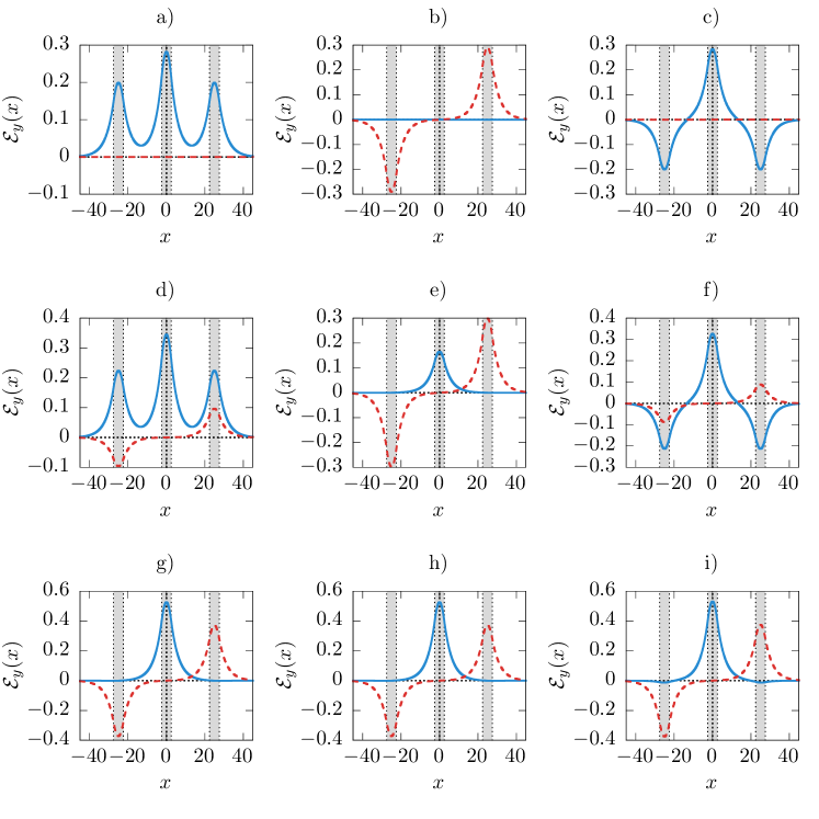
Figure 4: C-normalized stationary modes of the wave guide system for increasing non-Hermiticity parameter (from top to bottom) $\gamma=0.0\,\mathrm{cm}^{-1}$ (a) - c)), $\gamma=0.1\,\mathrm{cm}^{-1}$ (d) - f)), $\gamma=0.256802\,\mathrm{cm}^{-1}$ (g) - i)). The real part of the modes is illustrated by blue solid lines and the imaginary part by red dashed lines. From left to right there are shown the ground state mode and the two excited modes. The gray shaded areas represent the wave guides’ positions.

The modes depicted correspond to a system configuration according to Eqs. (8) and (9). In line with the system’s $\mathcal{PT}$ symmetry the real part of the modes is symmetric and the imaginary part is antisymmetric. With increasing $\gamma$ the imaginary part of the ground state mode and second excited mode grows while it is the real part that increases for the first excited mode. Close to the EP3 (bottom panel) we obtain the expected self-orthogonality phenomenon as the modes become essentially equal.

The progression of the propagation constants on the real axis towards the branch point according to Fig. 2 as well as the self-orthogonality phenomenon can be visualized experimentally by observing the beat length $L=2\pi/\Delta\beta$, where $\Delta\beta$ is the difference between two modes, of the power spectrum for the $\mathcal{PT}$-symmetric wave guide system. This can be observed for a non-stationary state. The power distribution

$$\left|E_{y}(x,z)\right|^{2}=\left|\frac{1}{\sqrt{3}}\sum_{i=1}^{3}\mathcal{E}_{i}(x)\mathrm{e}^{-\mathrm{i}\beta_{i}z}\right|^{2}$$ (19)

is taken, and displayed in Fig. 5 for three different values of $\gamma$.

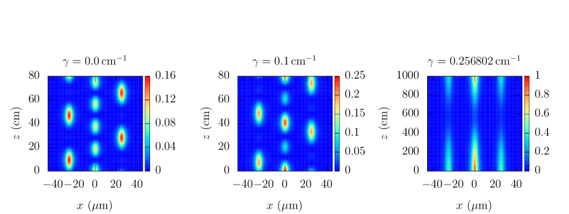
Figure 5: The power distribution for the propagating total field consisting of the three guided modes, see Eq. (19), for three values of the non-Hermiticity $\gamma$. With increasing values of $\gamma$ the corresponding beat length also increases. In addition an obvious rise in the intensity can be observed.

With increasing $\gamma$ the beat length also increases, which is a direct consequence of the movement of the propagation constants towards each other ($\Delta\beta$ becomes smaller). In the vicinity of the exceptional point the power spectrum no longer oscillates between the wave guides but rather pulses in all three wave guides simultaneously. Note the different length scales for the direction of propagation (i.e., $z$ axis). As the branch point is approached, i.e., $\Delta\beta\approx 0$ the beat length goes to infinity.

Furthermore we observe an increasing intensity of the power field for increasing values of the non-Hermiticity (see the corresponding color bars). This phenomenon is a consequence of the vanishing c norm when the branch point is approached. We note that the results shown in Fig. 4 and Fig. 5 for extended wave guides are in line with those of the simple three delta-functions model discussed in Heiss and Wunner (2016), confirming the validity of that model.

IV Further exceptional points in parameter space in the vicinity of the EP3

In this section we address an aspect associated with higher-order EPs that is related to the high parameter sensitivity of the eigenmodes in the vicinity of the EP3. It is a phenomenon that has so far attracted little attention but an awareness appears to be of utmost importance in an expected experimental confirmation. As is qualitatively discussed in Heiss (2008); Demange and Graefe (2012) a perturbation by only one of the parameters that were chosen to invoke the third-root branch point infers three eigenvalues to pop out in the energy plane from the EP3. In turn, the EP3 can be seen as a coalescence of two EP2s as the three eigenvalues – obtained from this perturbation – are still analytically connected. In fact, searching for singularities using some other parameter one finds two EP2s that sprout from the original EP3. Yet another parameter could then be used to force a coalescence of the two EP2s into a new and therefore shifted EP3.

This generic pattern turns out to be crucial for the identification of the EP3 via parameter space loops in our system. In the space of the physical parameters at hand curves of second-order and third-order exceptional points are found. These have a decisive effect on the permutation behavior of the modes.

To discover curves of EP2s in the system, and to clarify the points raised above we use the following condition similar to Eq. (7),

$$T_{21}=\frac{\partial T_{21}}{\partial\beta}=0\,.$$ (20)

As $T_{21}$ and its first derivative are complex valued functions, these equations give us four conditions that have to be fulfilled. Results are illustrated in Fig. 6

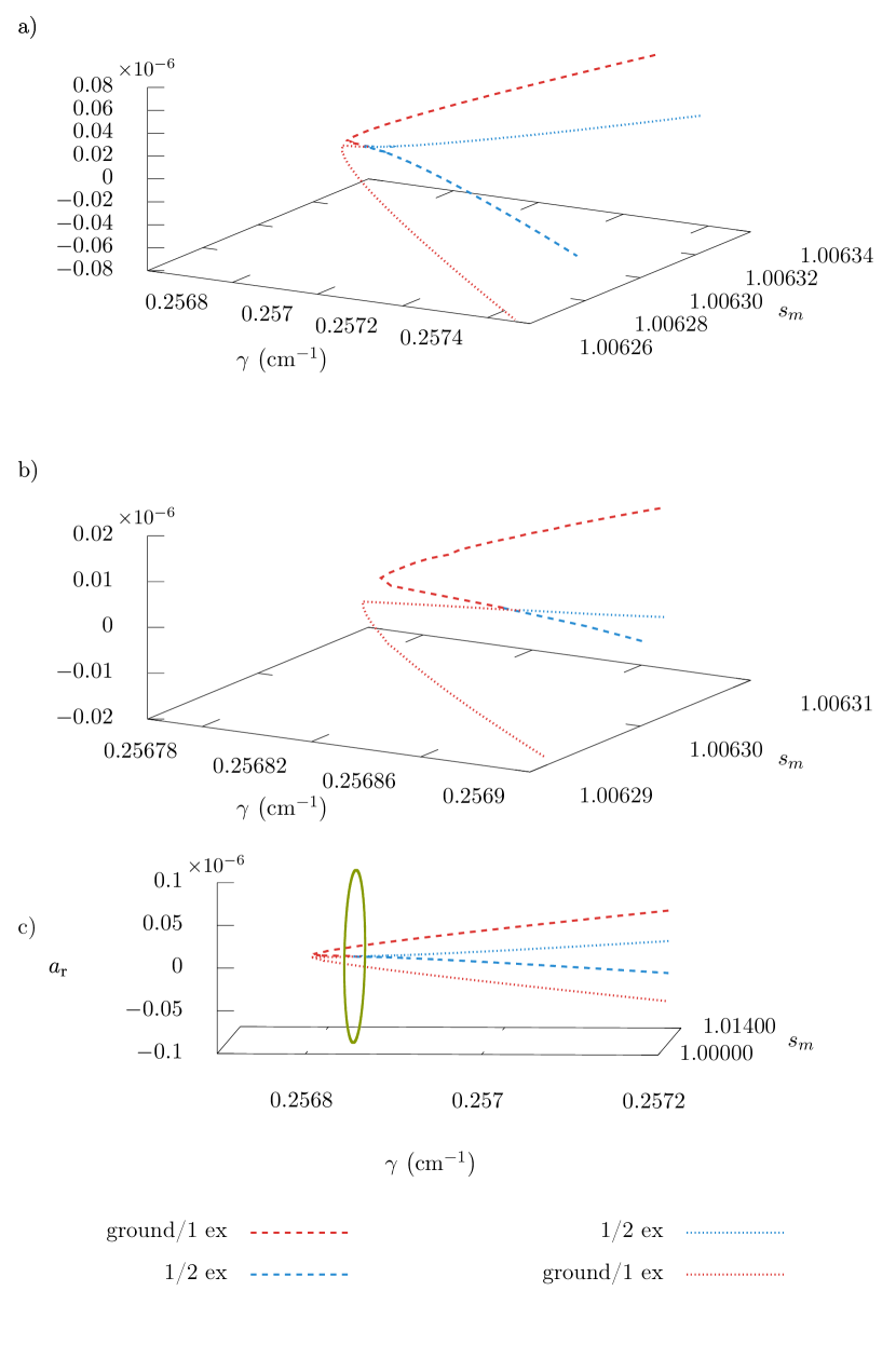
Figure 6: a) Curves denoting the positions in the three-dimensional parameter space $\left(\gamma,s_{m},a_{\mathrm{r}}\right)$ where EP2s are found for the wave guide system depicted in Fig. 1. The parameters $s_{1}^{\mathrm{EP3}}$, $s_{2}^{\mathrm{EP3}}$, $n_{m}^{\mathrm{EP3}}$, and $\Delta n$ are held fixed and for every $\gamma$ the values of ${\rm Re}\,(\beta),{\rm Im}\,(\beta),s_{m},a_{\mathrm{r}}$ are determined in a four-dimensional root search such that Eq. (20) is fulfilled. Branches of EP2s connecting either ground state and first excited mode or first and second excited mode sprout out from the EP3. b) Magnification of the space around the EP3 from which all lines originate. c) The circle in the parameter space (solid green line) in Fig. 3 circumscribes the EP3 and two EP2s formed by the branches of the ground state and the first excited state.

for a configuration of the system close to the EP3 given by Eqs. (8) and (9). While $s_{1}$, $s_{2}$, $n_{m}$, and $\Delta n$ are held fixed to their values at the EP3, $\gamma$ is varied in the range shown in the figures. For each value of $\gamma$ the parameters ${\rm Re}\,(\beta),{\rm Im}\,(\beta),s_{m},a_{\mathrm{r}}$ are determined in a four-dimensional root search. Projections of these lines on the two-dimensional parameter planes are shown in Fig. 7.

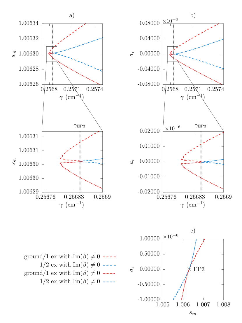
Figure 7: Projections of the two-dimensional curves of EP2s from Fig. 6 on the a) $\gamma$-$s_{m}$ b) $\gamma$-$a_{\mathrm{r}}$ and c) $s_{m}$-$a_{\mathrm{r}}$ planes.

While it is true that the threefold permutation identified in Fig. 3 clearly indicates the topological character of an EP3 one must keep in mind that the path around the EP3 circles in addition two second-order exceptional points, each of them formed by the ground and the first excited state. They belong to the red dashed and dotted lines. This explains why we do not find simple circles in Fig. 3 but rather the twisted curves that are caused by the presence of the EP2s (see also Fig. 7 in Menke et al. (2016) in a similar context). The effect of the two exceptional points included in the encircling is such that it does not affect the threefold permutation, i.e. the EP3 remains visible. In fact, both EP2s share the same sheet. It guarantees that the threefold permutation is not disturbed by their combined action. Of course the inclusion of the EP2s can be avoided altogether with a smaller circle. However, in an experiment it would be a rather laborious task to find and characterize all of the exceptional points thus avoiding the inclusion of unwanted EP2s.

The situation is different if $\gamma$ is chosen as one of the parameters for the circle. As can be extracted from Figs. 7 (a) and (b) the curves of EP2s only appear for non-zero values of the asymmetry parameter $a_{\mathrm{r}}$, which implies that the propagation constants become complex. At the position of the EP3, different EP2 lines originate. Along the blue dashed and dotted lines there are EP2s connecting the two excited modes that differ only in the signs of the corresponding imaginary parts of the propagation constants $\beta$. At the EP3 these imaginary parts vanish. The situation is similar along the red dashed and dotted lines, where the ground state mode and first excited mode are connected by an EP2. Since for $a_{\mathrm{r}}=0$ there exist no second-order exceptional points in the $\gamma$-$s_{m}$ plane nor in the $\gamma$-$a_{\mathrm{r}}$ plane we should, in principle be able to verify the EP3 by encircling. Yet it turns out that we observe EP2-like signatures.

If we allow for $a_{\mathrm{i}}=-b_{\mathrm{i}}\neq 0$ we obtain the results shown in Fig. 8. Instead of EP2s, signatures of EP3s can clearly be discerned (dashed lines). The corresponding propagation constants have a non-vanishing imaginary part as expected due to the broken $\mathcal{PT}$-symmetry. Again it should be possible to observe the EP3 signature in the $\gamma$-$s_{m}$ plane as well as in the $\gamma$-$a_{\mathrm{i}}/b_{\mathrm{i}}$ plane, respectively. However, only an EP2 signature is found. As in the example in the previous paragraph it could be possible that the EP3 interacts in such a way that the result is an EP2 signature Demange and Graefe (2012); Heiss (2016).

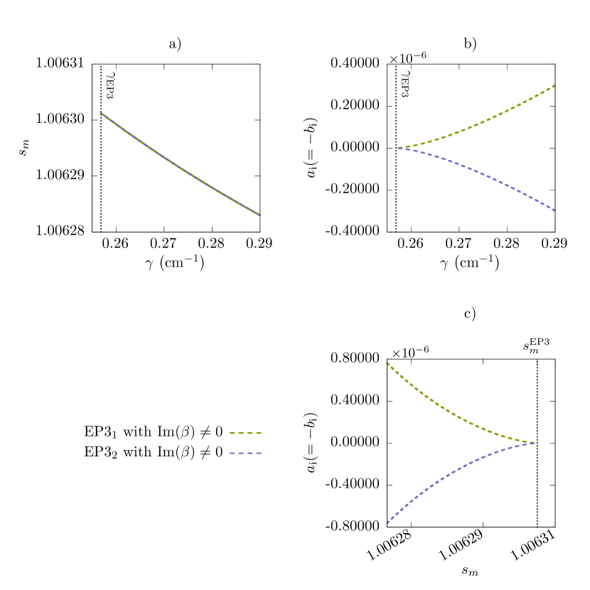
Figure 8: Curves denoting the positions in three-dimensional parameter space $\left(\gamma,s_{m},a_{\mathrm{i}}=-b_{\mathrm{i}}\right)$ where EP3s are found for the wave guide system depicted in Fig. 1. For every $\gamma$ ${\rm Re}\,(\beta),{\rm Im}\,(\beta),s_{m},a_{\mathrm{i}}=-b_{\mathrm{i}}$ are determined in a four-dimensional root search such that Eq. (20) is fulfilled while the other parameters of Eqs. (8) and (9) are held fixed. The figures contain the projections on the respective parameter planes. EP3s only exist in regions where $a_{\mathrm{i}}=-b_{\mathrm{i}}$ assumes non-zero values. The distributions differ in so far as they belong to different values of $a_{\mathrm{i}}=-b_{\mathrm{i}}$, which is also noticeable in mirrored imaginary parts of the propagation constants (not shown).

Thus there are different curves of EP2s and EP3s associated with the EP3 of the actual system. In this model there are specific parameter planes that are free from any EP2, yet they cannot be used to show the existence of the EP3 simply by encircling. Thus, the EP2 and EP3 lines have to be taken into account when the EP3 is supposed to be detected via its permutation behavior.

V Conclusion and Outlook

A system of three coupled $\mathcal{PT}$-symmetric wave guides can serve as a promising setup for an experimental verification of third-order exceptional points. Within an experimentally realizable parameter range for the system we have shown that the EP3 can be determined by simply varying a single parameter once the other parameters have been properly tuned. In our approach the non-Hermiticity parameter $\gamma$ is varied. The proper tuning of the other parameters appears to be the most challenging part in an experiment as even in numerical calculations, where the necessary high precision can be achieved, the task of finding the EP3 is rather demanding.

We feel that in a measurement of the power distributions of the total field for $\mathcal{PT}$-symmetric wave guides a direct visualization of the progression of the propagation constants towards the branch point can be obtained. It can be discerned by the increasing beat length when the EP3 is approached. In addition, using an appropriate encircling around the assumed position of the branch point it is possible to verify the threefold state exchange without even knowing the point’s exact position. Our numerical study can guide the approximate localization of the EP3 in an experimental setup.

Related to the verification of an EP3 by observing a threefold state exchange when encircling it in a suitably chosen parameter plane we have also shown that the branch point has further satellites of branches of EP2s or EP3s. From this we can extract a possible explanation for the complicated exchange behavior. They influence the permutation behavior and complicate the verification of the EP3 via its characteristic threefold state exchange. Thus, the beat length mentioned above might be the best choice for an experimental proof.

In a next step we will extend this one-dimensional optical system to a three-dimensional quantum mechanical one in terms of a Bose-Einstein condensate in a triple-well potential. This way we are going to propose a further, now really quantum mechanical, $\mathcal{PT}$-symmetric system for the verification of a third-order exceptional point.

GW and WDH gratefully acknowledge support from the National Institute for Theoretical Physics (NITheP), Western Cape, South Africa. GW expresses his gratitude to the Department of Physics of the University of Stellenbosch where this paper was finalized.

References

- Kato (1966) T. Kato, Perturbation theory for linear operators (Springer, Berlin, 1966).
- Heiss (2012) W. D. Heiss, J. Phys. A 45, 444016 (2012).
- Heiss and Sannino (1990) W. D. Heiss and A. L. Sannino, J. Phys. A 23, 1167 (1990).
- Heiss (2000) W. D. Heiss, Phys. Rev. E 61, 929 (2000).
- Hernández et al. (2006) E. Hernández, A. Jáuregui, and A. Mondragán, J. Phys. A 39, 10087 (2006).
- Lefebvre et al. (2009) R. Lefebvre, O. Atabek, M. Šindelka, and N. Moiseyev, Phys. Rev. Lett. 103, 123003 (2009).
- Cartarius et al. (2009) H. Cartarius, J. Main, and G. Wunner, Phys. Rev. A 79, 053408 (2009).
- Cartarius and Moiseyev (2011) H. Cartarius and N. Moiseyev, Phys. Rev. A 84, 013419 (2011).
- Gutöhrlein et al. (2013) R. Gutöhrlein, J. Main, H. Cartarius, and G. Wunner, J. Phys. A 46, 305001 (2013).
- Wiersig (2014) J. Wiersig, Phys. Rev. Lett. 112, 203901 (2014).
- Schwarz et al. (2015) L. Schwarz, H. Cartarius, G. Wunner, W. D. Heiss, and J. Main, Eur. Phys. J. D 69, 196 (2015).
- Menke et al. (2016) H. Menke, M. Klett, H. Cartarius, J. Main, and G. Wunner, Phys. Rev. A 93, 013401 (2016).
- Philipp et al. (2000) M. Philipp, P. von Brentano, G. Pascovici, and A. Richter, Phys. Rev. E 62, 1922 (2000).
- Dembowski et al. (2003) C. Dembowski, B. Dietz, H.-D. Gräf, H. L. Harney, A. Heine, W. D. Heiss, and A. Richter, Phys. Rev. Lett. 90, 034101 (2003).
- Dietz et al. (2007) B. Dietz, T. Friedrich, J. Metz, M. Miski-Oglu, A. Richter, F. Schäfer, and C. A. Stafford, Phys. Rev. E 75, 027201 (2007).
- Stehmann et al. (2004) T. Stehmann, W. D. Heiss, and F. G. Scholtz, J. Phys. A 37, 7813 (2004).
- Lawrence et al. (2014) M. Lawrence, N. Xu, X. Zhang, L. Cong, J. Han, W. Zhang, and S. Zhang, Phys. Rev. Lett. 113, 093901 (2014).
- Gao et al. (2015) T. Gao, E. Estrecho, K. Y. Bliokh, T. C. H. Liew, M. D. Fraser, S. Brodbeck, M. Kamp, C. Schneider, S. Hofling, Y. Yamamoto, F. Nori, Y. S. Kivshar, A. G. Truscott, R. G. Dall, and E. A. Ostrovskaya, Nature 526, 554 (2015).
- Doppler et al. (2016) J. Doppler, A. A. Mailybaev, J. Böhm, U. Kuhl, A. Girschik, F. Libisch, T. J. Milburn, P. Rabl, N. Moiseyev, and S. Rotter, Nature 537, 76 (2016).
- Xu et al. (2016) H. Xu, D. Mason, L. Jiang, and J. G. E. Harris, Nature 537, 80 (2016).
- Heiss (1999) W. D. Heiss, Eur. Phys. J. D 7, 1 (1999).
- Morse and Feshbach (1953) P. M. Morse and H. Feshbach, Methods of Theoretical Physics (McGraw-Hill, New York, 1953).
- Heiss and Wunner (2015) W. D. Heiss and G. Wunner, J. Phys. A 48, 345203 (2015).
- Lee et al. (2009) S.-B. Lee, J. Yang, S. Moon, S.-Y. Lee, J.-B. Shim, S. W. Kim, J.-H. Lee, and K. An, Phys. Rev. Lett. 103, 134101 (2009).
- Longhi (2010) S. Longhi, Phys. Rev. A 81, 022102 (2010).
- Guo et al. (2009) A. Guo, G. J. Salamo, D. Duchesne, R. Morandotti, M. Volatier-Ravat, V. Aimez, G. A. Siviloglou, and D. N. Christodoulides, Phys. Rev. Lett. 103, 093902 (2009).
- Chong et al. (2011) Y. D. Chong, L. Ge, and A. D. Stone, Phys. Rev. Lett. 106, 093902 (2011).
- Ge and Stone (2014) L. Ge and A. D. Stone, Phys. Rev. X 4, 031011 (2014).
- Chang et al. (2014) L. Chang, X. Jiang, S. Hua, C. Yang, J. Wen, L. Jiang, G. Li, G. Wang, and M. Xiao, Nat. Photon. 8, 524 (2014).
- Feng et al. (2014) L. Feng, Z. J. Wong, R.-M. Ma, Y. Wang, and X. Zhang, Science 346, 972 (2014).
- Hodaei et al. (2014) H. Hodaei, M.-A. Miri, M. Heinrich, D. N. Christodoulides, and M. Khajavikhan, Science 346, 975 (2014).
- Dembowski et al. (2001) C. Dembowski, H.-D. Gräf, H. L. Harney, A. Heine, W. D. Heiss, H. Rehfeld, and A. Richter, Phys. Rev. Lett. 86, 787 (2001).
- Brody (2014) D. C. Brody, J. Phys. A 47, 035305 (2014).
- Moiseyev (2011) N. Moiseyev, Non-Hermitian Quantum Mechanics (Cambridge University Press, Cambridge, 2011).
- Günther et al. (2007) U. Günther, I. Rotter, and B. F. Samsonov, J. Phys. A 40, 8815 (2007).
- Bender and Boettcher (1998) C. M. Bender and S. Boettcher, Phys. Rev. Lett. 80, 5243 (1998).
- Bender et al. (1999) C. M. Bender, S. Boettcher, and P. N. Meisinger, J. Math. Phys. 40, 2201 (1999).
- Znojil (1999) M. Znojil, Phys. Lett. A 264, 108 (1999).
- Jones and Moreira (2010) H. F. Jones and E. S. Moreira, Jr, J. Phys. A 43, 055307 (2010).
- Bender et al. (2012) C. M. Bender, V. Branchina, and E. Messina, Phys. Rev. D 85, 085001 (2012).
- Mannheim (2013) P. D. Mannheim, Fortschr. Phys. 61, 140 (2013).
- Graefe (2012) E.-M. Graefe, J. Phys. A 45, 444015 (2012).
- Dast et al. (2013) D. Dast, D. Haag, H. Cartarius, G. Wunner, R. Eichler, and J. Main, Fortschr. Phys. 61, 124 (2013).
- Abt et al. (2015) N. Abt, H. Cartarius, and G. Wunner, Int. J. Theor. Phys. 54, 4054 (2015).
- Gutöhrlein et al. (2015) R. Gutöhrlein, J. Schnabel, I. Iskandarov, H. Cartarius, J. Main, and G. Wunner, J. Phys. A 48, 335302 (2015).
- Graefe et al. (2008a) E. M. Graefe, U. Günther, H. J. Korsch, and A. E. Niederle, J. Phys. A 41, 255206 (2008a).
- Dast et al. (2016) D. Dast, D. Haag, H. Cartarius, and G. Wunner, Phys. Rev. A 93, 033617 (2016).
- Kreibich et al. (2016) M. Kreibich, J. Main, H. Cartarius, and G. Wunner, Phys. Rev. A 93, 023624 (2016).
- Dast et al. (2014) D. Dast, D. Haag, H. Cartarius, and G. Wunner, Phys. Rev. A 90, 052120 (2014).
- Bittner et al. (2014) S. Bittner, B. Dietz, H. L. Harney, M. Miski-Oglu, A. Richter, and F. Schäfer, Phys. Rev. E 89, 032909 (2014).
- Peng et al. (2014) B. Peng, S. K. Ozdemir, F. Lei, F. Monifi, M. Gianfreda, G. L. Long, S. Fan, F. Nori, C. M. Bender, and L. Yang, Nat. Phys. 10, 394 (2014).
- Bender et al. (2013) C. M. Bender, M. Gianfreda, Ş. K. Özdemir, B. Peng, and L. Yang, Phys. Rev. A 88, 062111 (2013).
- Makris et al. (2008) K. G. Makris, R. El-Ganainy, D. N. Christodoulides, and Z. H. Musslimani, Phys. Rev. Lett. 100, 103904 (2008).
- El-Ganainy et al. (2007) R. El-Ganainy, K. G. Makris, D. N. Christodoulides, and Z. H. Musslimani, Opt. Lett. 32, 2632 (2007).
- Schindler et al. (2011) J. Schindler, A. Li, M. C. Zheng, F. M. Ellis, and T. Kottos, Phys. Rev. A 84, 040101 (2011).
- Mostafazadeh and Mehri-Dehnavi (2009) A. Mostafazadeh and H. Mehri-Dehnavi, J. Phys. A 42, 125303 (2009).
- Mostafazadeh (2013a) A. Mostafazadeh, Phys. Rev. A 87, 063838 (2013a).
- Mostafazadeh (2013b) A. Mostafazadeh, Phys. Rev. Lett. 110, 260402 (2013b).
- Klaiman et al. (2008) S. Klaiman, U. Günther, and N. Moiseyev, Phys. Rev. Lett. 101, 080402 (2008).
- Rüter et al. (2010) C. E. Rüter, K. G. Makris, R. El-Ganainy, D. N. Christodoulides, M. Segev, and D. Kip, Nat. Phys. 6, 192 (2010).
- Graefe et al. (2008b) E. M. Graefe, U. Günther, H. J. Korsch, and A. E. Niederle, J. Phys. A 41, 255206 (2008b).
- Heiss (2008) W. D. Heiss, J. Phys. A 41, 244010 (2008).
- Demange and Graefe (2012) G. Demange and E.-M. Graefe, J. Phys. A 45, 025303 (2012).
- Heiss and Wunner (2016) W. D. Heiss and G. Wunner, J. Phys. A 49, 495303 (2016).
- Ge (2015) L. Ge, Phys. Rev. A 92, 052103 (2015).
- Ding et al. (2016) K. Ding, G. Ma, M. Xiao, Z. Q. Zhang, and C. T. Chan, Phys. Rev. X 6, 021007 (2016).
- Lin et al. (2016) Z. Lin, A. Pick, M. Lončar, and A. W. Rodriguez, Phys. Rev. Lett. 117, 107402 (2016).
- Jing et al. (2016) H. Jing, Ş. K. Özdemir, H. Lü, and F. Nori, “High-Order Exceptional Points and Low-Power Optomechanical Cooling,” (2016), arXiv:1609.01845 [quant-ph] .
- Dutta et al. (1992) N. K. Dutta, N. Chand, and J. Lopata, Applied Physics Letters 61, 7 (1992), http://dx.doi.org/10.1063/1.107620 .
- Susa (1995) N. Susa, IEEE Journal of Quantum Electronics 31, 92 (1995).
- Ganikhanov et al. (1999) F. Ganikhanov, K. C. Burr, D. J. Hilton, and C. L. Tang, Phys. Rev. B 60, 8890 (1999).
- Yeh (1988) P. Yeh, Optical Waves in Layered Media (Wiley, New York, 1988).
- Ge and Qi (2017) L. Ge and B. Qi, “Defect states emerging from a non-Hermitian flat band of photonic zero modes,” (2017), arXiv:1704.04713 [physics.optics] .
- Heiss (2016) W. D. Heiss, “Some features of exceptional points,” in Non-Hermitian Hamiltonians in Quantum Physics: Selected Contributions from the 15th International Conference on Non-Hermitian Hamiltonians in Quantum Physics, Palermo, Italy, 18-23 May 2015, edited by F. Bagarello, R. Passante, and C. Trapani (Springer International Publishing, Cham, 2016) pp. 281–288.