Selective Harvesting over Networks

Abstract

Active search on graphs focuses on collecting certain labeled nodes (targets) given global knowledge of the network topology and its edge weights (encoding pairwise similarities) under a query budget constraint. However, in most current networks, nodes, network topology, network size, and edge weights are all initially unknown. In this work we introduce selective harvesting, a variant of active search where the next node to be queried must be chosen among the neighbors of the current queried node set; the available training data for deciding which node to query is restricted to the subgraph induced by the queried set (and their node attributes) and their neighbors (without any node or edge attributes). Therefore, selective harvesting is a sequential decision problem, where we must decide which node to query at each step. A classifier trained in this scenario can suffer from what we call a tunnel vision effect: without any recourse to independent sampling, the urge to only query promising nodes forces classifiers to gather increasingly biased training data, which we show significantly hurts the performance of active search methods and standard classifiers. We demonstrate that it is possible to collect a much larger set of targets by using multiple classifiers, not by combining their predictions as a weighted ensemble, but switching between classifiers used at each step, as a way to ease the tunnel vision effect. We discover that switching classifiers collects more targets by (a) diversifying the training data and (b) broadening the choices of nodes that can be queried in the future. This highlights an exploration, exploitation, and diversification trade-off in our problem that goes beyond the exploration and exploitation duality found in classic sequential decision problems. Based on these observations we propose D³TS, a method based on multi-armed bandits for non-stationary stochastic processes that enforces classifier diversity, which outperforms all competing methods on five real network datasets in our evaluation and exhibits comparable performance on the other two.

1 Introduction

Active search on graphs Garnett et al (2011); Ma et al (2015); Wang et al (2013) is a technique for finding the largest number of target nodes – i.e., nodes with a certain label – in a network by querying nodes in a weighted graph, under a query budget constraint. Nodes have hidden labels but the network topology and edge weights are fully observable and any node can be queried at any time. Edge weights encode some form of node similarity that can be used to improve querying efficiency. Unfortunately, edge weights, network topology and node information are rarely available to be downloaded from one centralized place (except by the network’s owner, if any). As a result, today’s prevalent method to collect network data is to query neighbors of already queried nodes (crawling). Like active search on graphs, other similar techniques such as learning to crawl Gouriten et al (2014); Pant and Srinivasan (2005), also assume that edge weights between the queried nodes and their neighbors are observed. But in a variety of network crawling problems, such as crawling online social networks, (micro) blog networks, and citation networks, a node query often reveals only node attributes. This process poses an entirely new set of challenges for active search and other similar methods.

In this paper we introduce selective harvesting, where the goal is the same as in active search, but instead of assuming that the network topology is given, our node querying is subject to a partial and evolving understanding of the network More precisely, the knowledge about the network is restricted to the set of queried nodes and their connections to the rest of the network. Selective harvesting starts from a seed node (typically a target) and proceeds by querying nodes from the border set, i.e. neighbors of already queried nodes. Selective harvesting generalizes active sampling, a similar task where node attributes are not observed Pfeiffer III et al (2012). By leveraging information contained in these attributes, selective harvesting algorithms can attain better performance in applications of active sampling, such as (i) identifying students involved in academic dishonesty at a college/university; (ii) investigating securities fraud and (iii) identifying students who smoke/drink for intervention purposes. In these cases, target nodes are individuals that have a given trait.

Training a classifier for selective harvesting is a challenging task due to the fact that the classifier must be trained over observations that depend on previous choices of the same classifier, the hidden network topology, and the distribution of node features over the network. We call this the tunnel vision effect. Unlike active search, selective harvesting has no recourse to true randomness or sample independence that can ease the tunnel effect. Under partially observed networks, traditional active search methods perform quite poorly.

We discover that it is possible to collect a much larger set of target nodes by using a round robin scheme, which switches between different types of classifiers (e.g., Logistic Regression, Random Forests) when predicting labels in different steps. We show that this strategy collects more target nodes by (a) diversifying the training data and (b) broadening the choices of nodes that can be queried in the future. Based on these observations, we propose Directed Diversity Dynamic Thompson Sampling (D³TS), a Multi-Armed Bandit (MAB) algorithm for non-stationary stochastic processes that intelligently selects a classifier at each step to decide which neighbor to query. This is in sharp contrast with ensemble techniques, which combine predictions from several classifiers at each step. We show that these techniques (e.g., bagging and boosting) do not perform as well as D³TS due to the tunnel vision effect.

Unlike typical MAB problems, where there is a clear exploration and exploitation tradeoff, the standard MAB approach, which forces convergence to the “best classifier”, would be suboptimal in the presence of the tunnel vision effect. This gives rise to what we refer as exploration, exploitation, and diversification tradeoff. D³TS aims to induce continual diversification w.r.t. training data and potential node choices by using multiple distinct classifiers, which plays a similar role to sample independence and eases the tunnel vision effect.

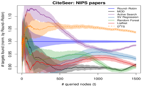
Figure 1: Lines show the (scaled) average number of targets found by round-robin, five naïve classifiers and D³TS against the total number of queries $(t)$. Shadows indicate 95% confidence intervals over 80 runs, each starting at a seed uniformly chosen from target population. Surprisingly, round-robin use of five classifiers (including poor-performing ones) outperforms any single classifier in the CiteSeer network. We also see that the best-performing active search method (Wang et al. Wang et al (2013)) has its relative accuracy eroded over time (and we will see why this is likely due to the tunnel vision effect). We include the proposed method (D³TS) results, which are consistently better than all competing methods for $t\geq 500$.

Interestingly, we find that even a round-robin selection of five distinct classifiers often performs better than just using the best classifier or the best active search method for each dataset. Consider simulation results shown in Figure 1 (the simulation is further explained in Section 6.1, for now we focus only on the overall results). Figure 1 shows the number of queries (x-axis) against the number of target nodes found in the CiteSeer paper co-citation network (NIPS papers as targets) normalized by the number of target nodes found by a round robin selection of five distinct simple classifiers (y-axis); the details of these simple classifiers are given in Section 3. Note that over time the cumulative gain of the best active search method for this dataset (Wang et al. Wang et al (2013)) slowly erodes until it is worse than the naïve round-robin approach. Our analysis shows that this erosion can be attributed to the tunnel vision effect. Each of the five simple classifiers when used on their own are consistently outperformed by the round-robin approach, and the best such classifiers also suffer from a performance erosion over time. In contrast, our proposed method, D³TS, consistently and significantly outperforms state-of-the-art methods, the round-robin approach, and naïve approaches. The contributions of this work are as follows:

1. Formulation and characterization of Selective Harvesting and Classifier Diversity: We introduce selective harvesting and show that state-of-the-art methods such as active sampling Pfeiffer III et al (2012); Bnaya et al (2013) and active search Garnett et al (2011); Wang et al (2013); Ma et al (2015) perform poorly in these settings. We show that switching between various classifiers is helpful to achieve greater performance. This works not because we are exploring classifiers in order to find the best one or because we are combining their predictions as an ensemble. Instead, the use of multiple classifiers – helps improve accuracy in two complementary ways. It achieves border set diversity, by exploring regions and thus avoiding remaining in a region where target nodes have been depleted. It also achieves training sample diversity, where diverse classifiers create enough diversity of observations to ease the tunnel vision effect.

2. Directed Diversity Dynamic Thompson Sampling (D³TS): we propose D³TS, a method for selective harvesting which combines different classifiers, and show that it consistently outperforms state-of-the-art methods. We evaluate the proposed framework on several real-world networks and observe that D³TS outperforms all tested methods on five out of seven datasets and exhibits similar performance on the other two.

Outline. In §2 we formalize the selective harvesting problem and present a generic algorithm for solving it. In §3 we describe existing and potential approaches to solve this problem and show that the tunnel vision effect hurts their performance. In §4 we investigate why classifier diversity – i.e., using multiple classifiers – can mitigate the tunnel vision effect. We propose D³TS in §5. Datasets and results of our evaluation are described in §6. Related work is described in §7. In §8 we discuss alternatives to the proposed method and explain why they cannot be applied or why they do not perform well. Last, our conclusions are presented in §9.

2 Problem Formulation

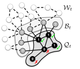
Figure 2: Representation of the search state over an unknown graph $\mathcal{G}$ after $t=4$ steps. Solid nodes and edges show the subgraph $\widetilde{\mathcal{G}}_{t}$. Black nodes represent queried nodes. Unknown labels of nodes in $\mathcal{B}_{t}$ are represented by a question mark “?”.

In this section we formalize the selective harvesting problem and introduce notation used throughout this work. Let $\mathcal{G}=(\mathcal{V},\mathcal{E})$ denote an undirected graph representing the network topology. Each node $v\in\mathcal{V}$ has $M$ attributes (domain-related properties of the nodes) encoded without loss of generality as an attribute vector $\mathbf{a}_{v}\in\mathbb{R}^{M}$.

In active search problems, the goal is to find a large set of nodes in $\mathcal{V}$ that satisfy a given search criterion (e.g., nodes that exhibit a given attribute) under the constraint that no more than $T$ nodes can be queried. The search criterion is a boolean function $f:\mathcal{V}\rightarrow\{0,1\}$. Formally, let $\mathcal{V}_{+}\subset\mathcal{V}$ be the set of all target nodes, i.e. all $v$ such that $f(v)=1$. We define node labels $y_{v}$ as

$$y_{v}=f(v)=\left\{\begin{array}[]{ll}1&\quad\text{ if $v\in\mathcal{V}_{+}$,}\\ 0&\quad\text{ otherwise.}\end{array}\right.\quad\forall v\in\mathcal{V}$$

Selective harvesting is a variant of active search. In active search, the topology is assumed to be known. In selective harvesting, the search is subject to a limited but evolving knowledge of the network. This knowledge is expanded by querying nodes in $\mathcal{V}$, which reveals their labels, neighbors and attribute vectors. A set of pre-queried nodes $\mathcal{Q}_{0}\subset\mathcal{V}$ is given as input (typically consisting of one target node). Subsequent queries are restricted to neighbors of already queried nodes.

At any step $t$, nodes belong to one of three sets: $\mathcal{Q}_{t}$, the set of previously queried nodes; $\mathcal{B}_{t}$, the set of neighbors of queried nodes that have not been queried (referred as border nodes or border set); or $\mathcal{W}_{t}$, the set of unobserved nodes, which are invisible to the algorithm. Figure 2 illustrates a snapshot of the search process (see caption for details).

Let $\widetilde{\mathcal{G}}_{t}=(\mathcal{Q}_{t},\widetilde{\mathcal{E}}_{t})$ denote the subgraph of $\mathcal{G}$ given by the subgraph induced by nodes in $\mathcal{Q}_{t}\cup\mathcal{B}_{t}$ minus edges in the subgraph induced by $\mathcal{B}_{t}$ (i.e., $\widetilde{\mathcal{G}}_{t}$ contains all edges between nodes in $\mathcal{Q}_{t}$ plus edges connecting $\mathcal{Q}_{t}$ to $\mathcal{B}_{t}$). The graph $\widetilde{\mathcal{G}}_{t}$ is the portion of the network visible at step $t$. In $\widetilde{\mathcal{G}}_{t}$, label $y_{v}$ is only known for nodes in $\mathcal{Q}_{t}$.

Generic solution. Given an initial input graph $\widetilde{\mathcal{G}}_{0}$, an algorithm for selective harvesting must decide at each step $t=1,\ldots,T$ what action to take, i.e., what border node $v\in\mathcal{B}_{t}$ to query, given the currently available network information. This action returns $v$’s label, attributes and connections, which is included as additional input to the search in step $t+1$. Node $v$ label (0 or 1) can be thought of as the payoff obtained by querying that node. The algorithm’s output is the list of target nodes found in $T$ steps. The best algorithm is the one that yields the largest total payoff, i.e., yields the largest number of target nodes.

3 Background

	PNB Pfeiffer III et al (2012)	SN-UCB1 Bnaya et al (2013)	MOD Avrachenkov et al (2014)	AS Wang et al (2013)	D3TS (ours)
Unknown network	✓	✓	✓	-	✓
Uses node features	-	-	-	-	✓
Unknown neighbor	-	-	-	-	✓
attributes
Fits model to evol-	-	✓	-	-	✓
ving observations
Scalable	-	✓	✓	✓	✓

Table 1: Comparison of heuristics for selective harvesting: Active Sampling (PNB), Social Network UCB1 (SN-UCB1), Maximum Observed Degree (MOD), and Active Search (AS).

In this section, we review methods for searching networks that can be used for or adapted to selective harvesting. These methods exploit correlation between labels of connected nodes to find targets. In addition, we review statistical models that could be used as an alternative (data-driven) approach. In contrast to existing methods, this approach can leverage node attributes by training a statistical model to infer the node’s label from the observed graph. As a slight abuse of terminology, we may refer to existing methods and base learners generically as classifiers, since both are used to infer border nodes’ labels.

3.1 Existing methods

A few works in the literature provide methods that can be used for or adapted to selective harvesting. A subclass of selective harvesting methods known as active sampling Pfeiffer III et al (2012); Bnaya et al (2013) does not account for node attributes. Our problem is closely related to the graph-theoretic myopic budgeted online covering problem Avrachenkov et al (2014); Khuller et al (2014); Borgs et al (2012). In this problem, all nodes are relevant (equivalently, all nodes are targets) and the task is to find a connected set of nodes that yields the largest cover (i.e., the largest set $\mathcal{Q}_{t}\cup\mathcal{B}_{t}$ set). The closest problem to ours is that addressed by active search on graphs Garnett et al (2011); Wang et al (2013); Ma et al (2015), where nodes have hidden labels but the topology and edge weights are fully observed and any node can be queried at any time. Algorithms for myopic budgeted online covering and active search can be adapted for selective harvesting; active sampling methods require little or no modification.

We adapt four representative methods of the above to selective harvesting: Active Sampling Pfeiffer III et al (2012) (PNB – in reference to the authors surnames), Maximum Observed Degree (MOD) Avrachenkov et al (2014), Social Network UCB1 (SN-UCB1) Bnaya et al (2013), and Active Search (AS) Wang et al (2013). Table 1 summarizes the key differences between these methods and the proposed method, D³TS.

Active Sampling (PNB): PNB is a representative algorithm from the class of active sampling approaches proposed in Pfeiffer III et al (2012). PNB estimates a border node’s payoff value $y_{v}$ using a weighted average of the payoffs of observed nodes two hops away from $v$, where weights are the number of common neighbors with $v$. Border nodes are included among these observed nodes, requiring all payoffs to be collectively estimated by a label propagation procedure based on Gibbs Sampling. PNB also tracks a running average of payoff values acquired from random jumps, which we do not allow in our simulations since these are not possible in selective harvesting. Please see Pfeiffer III et al (2012) for a detailed description of PNB’s parameters.

Social Network UCB1 (SN-UCB1): The SN-UCB1 search algorithm proposed in Bnaya et al (2013) divides border nodes into equivalence classes and samples from theses classes using a multi-armed bandit algorithm. Equivalence classes are composed of all border nodes connected to the same set of queried nodes. These classes are volatile: they split, disappear and appear over time, requiring the use of a variant of the UCB1 called VUCB1. Although this method learns about the equivalence classes, it does not learn a statistical model that can account for node attributes. Similar to selective harvesting, it assumes partial but evolving knowledge about the network.

Maximum Observed Degree (MOD): MOD is a myopic algorithm proposed in Avrachenkov et al (2014) to maximize the network cover as it explores a graph. MOD is the optimal greedy cover algorithm in a finite random power law network (under the Configuration Model Newman (2003)) with degree distribution coefficient either one or two. In our simulations we adapt MOD to select the border node with the maximum number of target neighbors in the queried set (ties are resolved randomly). From the expected excess degree results in Avrachenkov et al (2014) such border nodes are rich with target neighbors provided that the underlying network exhibits strong homophily with respect to node labels.

Active Search: this method, proposed by Wang et al. Wang et al (2013), attempts to find target nodes by assuming that labels are defined by a smooth function over the graph edges. To estimate the unknown labels, it attaches to each labeled instance a virtual node containing the instance’s label and then performs label propagation on the original graph. It assumes that the graph is known, which allows it to estimate the future impact of choosing a given border node. We adapt Active Search to run label propagation only on the observed graph.

3.2 Data-driven methods

A data-driven selective harvesting algorithm trains a statistical model to estimate the expected payoff $\mu_{t}(v)$ obtained from querying border node $v\in\mathcal{B}_{t}$, based on $v$’s relationship with the observed graph $\widetilde{\mathcal{G}}_{t}$ at step $t$. We encode this relationship as a “local” feature vector $\mathbf{x}_{v|\widetilde{\mathcal{G}}_{t}}$, which we describe next. Note that $v$’s features differ from $v$’s attributes (denoted by $\mathbf{a}_{v}$). Since $v$’s attributes are not observable until it is queried, we compute $v$’s local features from the observed graph $\widetilde{\mathcal{G}}_{t}$ to use as training data for base learners.

Feature Design

We define features for each border node in $v\in\mathcal{B}_{t}$. They are divided into:

• Pure structural features: observed degree and number of triangles formed with observed neighbors.

• Structure-and-attribute blends: number and fraction of target neighbors, number and fraction of triangles formed with two non-target (and with two target) neighbors, number and fraction of neighbors mostly surrounded by target nodes, fraction of neighbors that exhibit each node attribute, probability of finding a target exactly after two random walk steps from border node.

We build upon features typically used in the literature Robins et al (2007a, b). We also use a Random Walk (RW) transient distribution to build features: we consider the expected payoff observed by a RW that departs from node $u\in\mathcal{B}_{t}$ and performs two steps, given by

$$x_{u|\widetilde{\mathcal{G}}_{t}}^{\textrm{(RW)}}=\frac{\sum_{(u,v)\in\widetilde{\mathcal{E}}_{t}}\sum_{(v,w)\in\widetilde{\mathcal{E}}_{t},w\in\mathcal{Q}_{t}}y_{w}}{C_{u|\widetilde{\mathcal{G}}_{t}}}$$ (1)

where $C_{u|\widetilde{\mathcal{G}}_{t}}$ is the number of such paths of length two in $\widetilde{\mathcal{G}}_{t}$. Note that the RW is not restricted to the immediate neighbors of $u$. Also, this is not an average among the nodes two hops away from $u$; this feature depends on the connectedness of the border node’s neighborhood in the observed graph.

Base Learners

The feature vector described above can be given as input to any learning method able to generate a ranking of border nodes. We consider classification, regression and ranking methods as suitable candidates for this task. The classification representatives include Logistic Regression and Random Forests, because they provide ways to rank border nodes according to how confident the model is that each border node is a target. Exponentially Weighted Least Squares (EWLS) and Support Vector Regression are included by modeling the task as a regression problem, and the list-wise learning-to-rank method ListNet Cao et al (2007) for directly outputting ranks. We briefly describe EWLS and ListNet below and refer the reader to Friedman et al (2009) for descriptions of other methods.

Exponentially Weighted Least Squares (EWLS): computes weights $\mathbf{w}$ that, given a forgetting factor $0\ll\beta\leq 1$ and regularization parameter $\lambda$, minimize the loss function

$$\sum_{i=1}^{t}\beta^{t-i}|y_{t}-\mathbf{x_{t}}^{\top}\mathbf{w}|^{2}+\beta^{t}\lambda\|w\|^{2}.$$

EWLS gives more weight to recent observations. The weights $\mathbf{w}$ are suitable for fast online updates (Liu et al, 2011, Section 4.2). Setting $\beta=1$ reduces EWLS to $\ell_{2}$-regularized Linear Regression.

ListNet: This is a representative method from the list-wise approaches for learning to rank (a Machine Learning task where the goal is to learn how to rank objects according to their relevance to a query) Cao et al (2007). It assumes that the observed ranking $\bm{\pi}$ is a random variable that depends on the objects’ scores (where $\pi_{1}$ is the top-ranked object). The scores are determined by a neural network that is trained by minimizing the K-L divergence between the probability distribution over $\bm{\hat{\pi}}$ and the probability distribution over a ranking $\bm{\pi}$ derived from ground-truth scores. In our context, $P(\bm{\pi})$ is given by

$$P(\bm{\pi}=\langle\pi_{1},...,\pi_{|\mathcal{B}_{t}|}\rangle)=\prod_{i=1}^{|\mathcal{B}_{t}|}\left[\exp(y_{\pi_{i}})/\sum_{j=i}^{|\mathcal{B}_{t}|}\exp(y_{\pi_{j}})\right].$$

Since the goal is not to predict the object-wise relevance, all of the statistical power of this method goes into learning the ranking.

As with any learning approach, in the “small data” regime (few observations collected) a base learner may perform worse than heuristic methods that assume homophily w.r.t. node labels. To mitigate issues related to fitting a learner to few observations and yet allow a fair comparison with the heuristic methods, we query the first $20$ nodes using MOD.

4 Tunnel Vision and the power of Classifier Diversity

In selective harvesting the goal is to find the most number of target nodes with a limited query budget. This requires methods to try to sample only promising target nodes, which causes a given classifier to gather increasingly biased training data, a phenomenon that we call tunnel vision effect. Unfortunately, it is unlikely that we can find a method which provably compensates for this bias in our training data, $\mathcal{Q}_{t}$. Even if we query border nodes randomly at each step, we cannot determine the probability of seeing any given node in the border set $\mathcal{B}_{t}$, as this would require assessing the probability of all possible sample paths from the given seed nodes, which includes paths containing nodes not yet observed, i.e., nodes in $\mathcal{W}_{t}$ in Figure 2, an unfeasible task as we do not know the network topology. This is likely why active search and base learners by their own do not work well for selective harvesting tasks. This is also why importance weighted sampling Beygelzimer et al (2009) cannot be used to remove the bias in these tasks.

Methods	Datasets (budget $T$)
	CS	DBP	WK	DC	KS	DBL	LJ
	(1500)	(700)	(400)	(100)	(700)	(1200)	(1200)
PNB	833.2∗	260.6∗	107.7∗	24.3∗	178.3∗	599.5∗	632.4∗
SN-UCB1	568.9∗	272.3∗	71.8∗	23.2∗	133.2∗	399.1∗	573.7∗
MOD ✓	746.8∗	403.0∗	140.9∗	35.7∗	159.6∗	580.3∗	584.1∗
Active Search ✓	808.9∗	412.2∗	143.4	22.6∗	215.3∗	684.9∗	654.2∗
Logistic Regression	764.5∗	452.5	86.2∗	35.8	122.1∗	744.4	732.0
Random Forest ✓	738.5∗	454.0∗	127.2∗	37.2	215.6∗	725.4	728.3∗
EWLS	808.2∗	462.4	82.5∗	35.2∗	142.3∗	656.9∗	694.4∗
SV Regression ✓	770.6∗	456.3∗	85.0∗	37.6	205.3∗	757.1∗	736.1
ListNet ✓	742.0∗	448.0∗	92.5∗	34.4∗	146.3∗	730.7	742.8
Round-Robin (all ✓)	822.2∗	454.5∗	135.3∗	37.3	234.9∗	696.0∗	716.0∗
D3TS (all ✓)	851.2	464.0	144.7	37.9	247.6	729.5	737.3
Target population size	1583	725	202	56	1457	7556	1441

Table 2: Average number of targets found by each method after $T$ queries based on 80 runs. Datasets. CS: CiteSeer, DBP: DBpedia, WK: Wikipedia, DC: DonorsChoose, DBL: DBLP, KS: Kickstarter and LJ: LiveJournal. Budget $T$ is respectively set to number of targets $\times 1,\times 1,\times 2,\times 2,\times\frac{1}{2},\times\frac{1}{6},\times\frac{5}{6}$ truncated to hundreds. First four rows correspond to existing methods; five subsequent rows are base learners. Round-Robin and D³TS combine methods indicated by (✓). Means whose difference to D³TS’s is statistically significant at the 95% confidence level are indicated by (^∗). Best two results on each dataset are shown in bold. Parameters. PNB: same as in Pfeiffer III et al (2012); Active Search: same as in Wang et al (2013); ELWS: $\beta=.99$, $\lambda=1.0$; Logistic Regression and SV Regression: penalty $C$ set using fast heuristic implemented in R package LiblineaR Helleputte (2015); Random Forest: no. variables $=\sqrt{\textrm{no. features}}$, number of trees $=100$ (DBL and LJ use classical decision trees for speed, others use conditional inference trees Hothorn et al (2006)); ListNet: no. iterations $=100$, tolerance $=10^{-5}$.

To demonstrate the tunnel vision effect and show how classifier diversity can mitigate it, we conduct a large set of simulations. We simulate searches using four heuristics – MOD, PNB, Social Network-UCB1 (SN-UCB1) and Active Search, five base learners – Logistic Regression, Exponentially Weighted Least Squares (EWLS), Support Vector Regression, Random Forest and ListNet on seven networks and summarize the results in Table 2 (network datasets and target populations are described in Section 6.1). We observe that the best classifier varies across datasets. More surprisingly, the best classifier for one dataset may be the worst for another (see Active Search on Wikipedia and on DonorsChoose).

We then consider a set of classifiers $\mathcal{M}$ that typically exhibit good performance and cycle between them during the search, in a Round-Robin (RR) fashion. Based on Table 2, we pick $\mathcal{M}$={MOD, Active Search, Support Vector Regression, Random Forest, ListNet}. We use this set of classifiers throughout the rest of this paper, unless otherwise noted. One might expect RR’s performance to be the average of the performance results yielded by the standalone counterparts, but this is not the case. Interestingly, switching classifiers at each step outperforms the best classifier in $\mathcal{M}$ on the CiteSeer and Kickstarter datasets, and finds at least 92% as many target nodes as the best classifier on other datasets. In what follows we investigate why the use of multiple classifiers can improve selective harvesting’s performance.

4.1 Leveraging diversity through the use of multiple classifiers

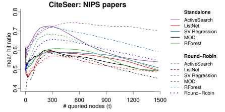
Figure 3: Round-robin can have higher hit ratios for each of its classifiers than their standalone counterparts.

We observe that RR outperforms all five classifiers in $\mathcal{M}$ on CiteSeer (Table 2). Consequently, at least one of them must perform better under RR than on its own. In order to identify which ones do, we show in Figure 3 the hit ratio – number of target nodes found divided by number of queries performed using each classifier up to time $t$ – under RR and when used by itself, averaged over 80 runs. Interestingly, after $t=400$ all classifiers exhibit similar (relative difference $\leq 10\%$) or better performance under RR than when used alone.

We propose two hypotheses to explain this performance improvement:

1. Border Hypothesis: RR explores regions of the graph containing more targets that are likely to be scored high by a classifier, i.e. RR infuses diversity in the border set.

2. Training Hypothesis: Observations from different classifiers can be used to train the others to generalize better and cope with self-reinforcing sampling biases, i.e., diversity in the training set produces a classifier that is better at finding target nodes.

Note that these hypotheses are not mutually exclusive. In what follows, we perform controlled simulations to isolate and study each hypothesis.

Training set diversity directly impacts model parameters. Model parameters, in turn, determine how the border set will change. Therefore, to assess the impact of training set diversity we must hold the border set diversity constant and vice-versa. This is the key idea behind the two controlled sets of simulations described next. To perform them, we instrumented our simulator to load, from another simulation run, (i) the feature vector $\mathbf{x}_{\sigma_{t}|\widetilde{\mathcal{G}}_{t}}$ of node $\sigma_{t}$ queried in step $t$, and label $y_{\sigma_{t}}$, and (ii) the observed graph $\widetilde{\mathcal{G}}_{t}$ at each step $t$. In what follows, we show the results obtained using the support vector regression (SVR) model. We denote node $\sigma_{t}$’s feature vector and label simply by $\mathbf{x}_{t}$ and $y_{t}$, respectively, to make it easier to follow.

(a) Simulations for studying Border Hypothesis

(b) Simulations for studying Training Hypothesis

Figure 4: (a) We study the Border Hypothesis by recreating the sequence of SVR models from the original simulation run (stage 1) and using them to query nodes on a sequence of observed graphs collected using round-robin (stage 2). (b) We study the Training Hypothesis by recreating the sequence of observed graphs from the original simulation run (stage 1) and using a SVR trained on the samples collected using round-robin (stage 2) to query nodes.

Border Hypothesis. Our experiment consists of three stages (Fig. 4a). First, we store the sequence of observations (i.e., pairs feature vector, label) $\mathcal{O}_{\mathrm{SVR}}=\left((\mathbf{x}_{1},y_{1}),\ \ldots,(\mathbf{x}_{T},y_{T})\right)$ corresponding to nodes queried when searching a network dataset $\mathcal{D}$ using SVR. Second, we store the sequence of observed graphs $\widetilde{\mathcal{G}}_{\mathrm{RR}}=\left(\widetilde{\mathcal{G}}_{1},\ldots,\widetilde{\mathcal{G}}_{T}\right)$ when searching $\mathcal{D}$ by cycling between models in the set $\mathcal{M}$. Last, we simulate another SVR-based search on $\mathcal{D}$, loading the observed graph at each time step $t$ from $\widetilde{\mathcal{G}}_{\mathrm{RR}}$. However, instead of training the SVR model with observations collected on that run (which most likely differ from those collected during the first stage), we gradually feed it with observations from $\mathcal{O}_{\mathrm{SVR}}$, one for each simulation step $t$. Therefore, we will reproduce the sequence of classifiers from the first stage, but subject to a different sequence of observed graphs.

Training Hypothesis. As before, our experiment consists of three stages (Fig. 4b). In the first stage, we store the sequence of observed graphs $\widetilde{\mathcal{G}}_{\mathrm{SVR}}=\left(\widetilde{\mathcal{G}}^{\prime}_{1},\ldots,\widetilde{\mathcal{G}}^{\prime}_{T}\right)$ when searching $\mathcal{D}$ using a SVR model. Second, we store the sequence of observations $\mathcal{O}_{\mathrm{RR}}=\left((\mathbf{x}_{1}^{\prime},y_{1}^{\prime}),\ldots,(\mathbf{x}_{T}^{\prime},y_{T}^{\prime})\right)$ collected when searching $\mathcal{D}$ by cycling among classifiers in $\mathcal{M}$. Last, we simulate another SVR-based search, loading the observed graph at each time step $t$ from $\widetilde{\mathcal{G}}_{\mathrm{SVR}}$, but feeding it observations from $\mathcal{O}_{\mathrm{RR}}$, one by one. Hence, the classifier is fit to a different set of observations, but the search is subject to the same sample path as the SVR-based search from the first stage.

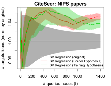
Figure 5: SVR classifier and two ways to ease the tunnel vision effect: border set diversity and training set diversity improve performance by ensuring greater diversity in query choices and by diversifying the training data, respectively.

Figure 5 contrasts the average number of target nodes found by the original SVR-based search on CiteSeer against those obtained in each set of simulations based on 80 runs. The 95% confidence intervals for the mean at $t=700$ are $[393.8,413.1]$, $[416.6,427.5]$ and $[417.1,436.7]$. These statistics corroborate the hypotheses that the border set and the training data collected by the round-robin policy contribute to improving the performance of the SVR model.

Intuitively, when a base learner is fit to the nodes it queried, it tends to specialize in one region of the feature space and the search consequently only explores similar parts of the graph, which can severely undermine its potential to find target nodes. One way to mitigate this overspecialization would be to sample nodes from the border set probabilistically, as opposed to deterministically querying the node with the highest score. This alternative is investigated in Appendix B, where the ranking associated with each classifier is mapped into a probability distribution. The results show no significant performance improvement over those obtained when a single classifier chooses nodes to query deterministically.

The round-robin policy infuses diversity in the training set without sacrificing performance. This diversity is achieved by “asking another classifier” what is the best node to query at a given step. In scenarios where all classifiers would have performed reasonably well if used alone, learning from another’s classifier query is likely to improve one classifier’s ability to find targets, especially when they disagree.

Yet, different classifiers inherently exhibit different performances on a dataset. Clearly, we want to choose more accurate classifiers more often, but in order to do so, three challenges must be addressed:

1. We do not know a priori which classifiers are more accurate on a dataset;

2. Classifiers’ accuracy varies as their parameters are updated and the border set changes;

3. Continual exploration must be ensured, since converging to an arm would make the search more susceptible to the tunnel vision effect.

Challenge (1) is typically addressed by Multi-Armed Bandit (MAB) algorithms. Challenge (2) constrains the set of possible MAB algorithms to those designed for MAB problems with non-stationary reward distributions. Challenge (3) is specific to selective harvesting (the exploration-exploitation-diversification trade-off). In the following section, we propose a method that addresses all these challenges. We call it Directed Diversity Dynamic Thompson Sampling because it is based on the Dynamic Thompson Sampling algorithm for MAB problems and because it leverages diversity in a “directed way” as opposed to randomly sampling nodes.

5 Directed Diversity Dynamic Thompson Sampling (D³TS)

This section is divided in two parts. First, we discuss the relationship between selective harvesting and multi-armed bandits. Then, in the light of this discussion, we propose the D³TS algorithm.

5.1 Relationship between Selective harvesting and Multi-Armed Bandits

Selective harvesting with multiple classifiers can be cast as a Multi-Armed Bandit (MAB) problem. In a MAB problem, a forecaster is given the number of arms $K$ and the number of rounds $T$. For each round $t$, nature generates a payoff vector $\mathbf{r}_{t}=(r_{1,t},\ldots,r_{K,t})\in[0,1]^{K}$ unobservable to the forecaster. The forecaster chooses an arm $I_{t}\in\{1,\ldots,K\}$ and receives payoff $r_{I_{t},t}$, with the other payoffs hidden. The goal is to maximize the cumulative payoff obtained. MAB problems can be classified according to how the payoff vector is generated. In stochastic bandit problems, each entry $r_{i,t}$ in the payoff vector is sampled independently, from an unknown distribution $\nu_{i}$, regardless of $t$. In adversarial bandit problems, the payoff vector $\mathbf{r}_{t}$ is chosen by an adversary which, at time $t$, knows the past, but not $I_{t}$. Stochastic and adversarial bandits do not cover the entire problem space, as the payoff vector distribution may vary over time in a less arbitrary way than in adversarial bandits. In stochastic bandit problems with non-stationary distributions or dynamic bandit problems, the mean payoff vector can evolve according to random shocks or change at pre-determined points in time. MAB problems may also include context, which provides the forecaster with side information about the optimal action at a given step. In contextual bandits, a context $\mathbf{x}_{a,t}$ is drawn (from some unknown probability distribution) for each action $a\in\mathcal{A}_{t}$ available in step $t$. The context may be provided explicitly or through recommendations of a set of experts.

In selective harvesting, the sequential decision problem consists of choosing the node to query at each step, given recommendations from several models. There are two ways of mapping selective harvesting to a MAB problem. The first (and simplest) mapping is context-free. Each model is represented by an arm (i.e., the problem reduces to one of choosing a model at each time step). Models are treated as black boxes that will “internally” query a node and return the node’s label. The queried node’s label is seen as the model’s payoff. The second mapping falls into the class of contextual bandits. Each border node represents an action and each model represents an expert that provides recommendations on how to choose the actions. Node features correspond to action contexts, which are used by the experts to compute their recommendations.

Despite the potential advantage of accounting for node features directly and combining the advice of several models, most algorithms for contextual bandits assume fixed and small (relative to the time horizon) sets of actions, whereas the border set is dynamic and potentially orders of magnitude larger than the query budget. Among context-free bandits, we claim that algorithms for stochastic bandits with non-stationary distributions are the best candidates for combining classifiers in selective harvesting, as we observe that the average hit ratio can drift over time (Fig. 3). While adversarial bandits allow payoff distributions to change arbitrarily, they cannot exploit the fact that the mean payoff evolves in a well-behaved manner. A thorough comparison of several bandit algorithms described in Appendix C supports our claim. Our comparison includes the Exp4 and Exp4.P algorithms for contextual bandits, which combine the prediction of all classifiers in a similar way that traditional ensemble methods do.

Algorithm 1 D³TS (budget $T$, model set $\mathcal{M}$, threshold $C\geq 2$)

1:$\triangleright$ Assume $\mathcal{B}_{t}$ is updated after each iteration.

2:for $t$ in $1,\ldots,T$ do

3:     for $k$ in $1,\ldots,|\mathcal{M}|$ do

4:         $\hat{r}_{t}^{(k)}\sim\mbox{Beta}(\alpha_{k},\beta_{k})$      

5:     $I_{t}={\arg\max}_{k\in 1,\ldots,K}\hat{r}_{t}^{(k)}$

6:     $\hat{\mathbf{y}}=$ estimate payoffs using classifier $I_{t}$ and $\widetilde{\mathcal{G}}_{t}$

7:     $b=\arg\max_{v\in\mathcal{B}_{t}}\hat{y}_{v}$

8:     $r_{t}=y_{b}=$ query$(b)$

9:     if  $\alpha_{I_{t}}+\beta_{I_{t}}<C$  then

10:         $\alpha_{I_{t}}=\alpha_{I_{t}}+r_{t}$

11:         $\beta_{I_{t}}=\beta_{I_{t}}+(1-r_{t})$

12:     else

13:         $\alpha_{I_{t}}=(\alpha_{I_{t}}+r_{t})\times C/(C+1)$

14:         $\beta_{I_{t}}=(\beta_{I_{t}}+(1-r_{t}))\times C/(C+1)$      

15:     $\mathcal{M}=$ update or retrain classifiers given new point $(x_{b|\widetilde{\mathcal{G}}_{t}},y_{b})$

5.2 Proposed algorithm

For the reasons above, we adapt the Dynamic Thompson Sampling (DTS) algorithm Gupta et al (2011) proposed for MABs with non-stationary distributions to the selective harvesting problem. DTS is based on the Thompson Sampling (TS) algorithm for stochastic MABs, where binary outcomes associated with each arm $k=1,\ldots,K$ are modeled as Bernoulli trials. The uncertainty on the probability parameter associated with arm $k$ is typically modeled as a distribution $\mbox{Beta}(\alpha_{k},\beta_{k})$. The Beta distribution is the conjugate prior for the Bernoulli distribution (thus providing computational savings on Bayesian updates). TS performs exploration by choosing arms probabilistically, according to samples drawn from the corresponding distributions. More precisely, at step $t$, TS samples $\hat{r}_{t}^{(k)}\sim\mbox{Beta}(\alpha_{k},\beta_{k})$ and selects the arm with the largest sample, i.e., $I_{t}=\arg\max_{k\in 1,\ldots,K}\hat{r}_{t}^{(k)}$. Given the binary payoff $r_{t}$ received after selecting arm $I_{t}$, the distribution parameters are updated according to the Bayesian rule, i.e., $\alpha_{I_{t}}=\alpha_{I_{t}}+r_{t}$ and $\beta_{I_{t}}=\beta_{k}+(1-r_{t})$. In essence, DTS normalizes arm $k$’s parameters such that $\alpha_{k}+\beta_{k}\leq C$, where $C$ is a bounding parameter. We adapt DTS in two senses: (i) we combine DTS with the steps needed to perform search in selective harvesting problems and (ii) we set the threshold $C$ to a much smaller value than the ones used in Gupta et al (2011), which allows us to incur more diversity. This highlights an exploration, exploitation and diversification tradeoff in selective harvesting that goes beyond the duality found in classic MAB problems, as simply converging to one arm would be suboptimal. The pseudo-code for D³TS is shown in Algorithm 1. In what follows we compare D³TS against all approaches for selective harvesting discussed in Section 3.

6 Simulations

This section describes the datasets used in our simulations, together with simulation results and comparisons with baseline methods.

6.1 Datasets

To evaluate the above search methods, we use seven datasets corresponding to undirected and unweighted networks containing node attributes. In the following we describe each of the datasets summarized in Table 3. Basic statistics for each network are shown in Table 4.

Dataset	nodes	edges	node attributes	target nodes
DBpedia	places	hyperlinks	place type	admin. regions
CiteSeer	papers	citations	venues	top venue
Wikipedia	wikipages	links	topics	OOP pages
Kickstarter	donors	co-donors	backed projects	DFA donors
DonorsChoose	donors	co-donors	awarded projects	$P$ donors
LiveJournal	users	friendship	enrolled groups	top group
DBLP	authors	co-authorship	conference	top conference

Table 3: High-level description of each network.

Dataset	$|\mathcal{V}|$	$|\mathcal{E}|$	$M$	$|\mathcal{V}_{+}|/|\mathcal{V}|$
DBpedia	5.00K	26.6K	5	14.5%
CiteSeer	14.1K	42.0K	10	13.1%
Wikipedia	5.27K	64.6K	93	3.83%
Kickstarter	27.8K	2.77M	180	5.27%
DonorsChoose	1.15K	6.60K	284	4.96%
LiveJournal	4.00M	34.7M	5K	0.04%
DBLP	317K	1.05M	5K	2.38%

Table 4: Basic statistics of each network: $|\mathcal{V}|$ (number of nodes), $|\mathcal{E}|$ (number of edges), $M$ (number of attributes) and $|\mathcal{V}_{+}|/|\mathcal{V}|$ (fraction of target nodes).

The first three datasets have been used as benchmarks for Active Search Wang et al (2013); Ma et al (2015). Despite the fact that Active Search assumes that the network topology is known, we can use these datasets to evaluate active search methods by only revealing parts of the graph as the search proceeds. We define the target population as in the Active Search work.

DBpedia: A network of 5000 populated places from the DBpedia ontology formed by linking pairs whose corresponding Wikipedia pages link to each other, in either direction. Places are marked as “administrative regions”, “countries”, “cities”, “towns” or “villages”. Target nodes are the “administrative regions”.

CiteSeer: A paper citation network composed of the top 10 venues in Computer Science. Papers are annotated with publication venue. Target nodes are the NIPS papers.

Wikipedia: A web-graph of wikipages related to programming languages. Pages are annotated with topics obtained by thresholding a pre-computed topic vector Wang et al (2013). Target nodes are webpages related to “object oriented programming”.

Two network datasets from the Stanford SNAP repository Leskovec and Krevl (2014) typically used to validate community detection algorithms are also used. We label nodes belonging to the largest ground-truth community as targets. Other community memberships are used to define a binary attribute vector $\mathbf{a}_{v}\in\{0,1\}^{M}$ for all $v\in V$.

LiveJournal: A blog community with OSN features, e.g.: users declare friendships and create groups that others can join. Users are annotated with the groups they joined.

DBLP: A scientific collaboration network where two authors are connected if they have published together. Authors are annotated with their respective publication venues.

Last, we use datasets containing donations to projects posted on two online crowdfunding websites. To assess the performance of each classifier in low correlation settings, we build a social network connecting potential donors where edges are weak predictors of whether or not neighbors of a donor will also donate. We label nodes as targets if they donated to a specific campaign. Historical donation data prior to that is used to build the network and define node attributes.

Kickstarter(.com): An online crowdfunding website. This dataset was collected by GitHub user neight-allen and consists of 3.04M donors that together made 5.87M donations to 87.3K projects. We create a donor-to-donor network by connecting donors that donated to the same projects in the past. More precisely, we assume that backers of small unsuccessful campaigns (between 100 and 600 backers) are all connected in a co-donation network – say, their names are published on the campaign’s website. We choose campaigns with few donors so that the resulting network is sparse and the network discovery problem challenges D³TS. Our dataset has 180 small unsuccessful projects between 04/21/2009 and 05/06/2013, containing a total of 27.8K donors. We then choose the 2012 project (denoted DFA) that has the largest number of donors in our dataset. The goal of the recruiting algorithm is to recruit the 2012 DFA donors through the donor-to-donor network of past donations (2009–2011).

DonorsChoose(.org): An online crowdfunding website where teachers of US public schools post classroom projects requesting donations (e.g., for a science project). The dataset is part of the KDD 2014 Cup containing 1.29M donors that together made 3.10M donations to 664K projects from 57K schools. Donations include information such as donor location, donation amount, awarded project, among other node features. As donors tend to be loyal to the same schools, we focus on the school that received the most donations in the dataset. We use projects from 2007 to 2012 to construct a donor-to-donor network where an edge exists between two donors if they donated to the same project less than 48 hours apart. We then select the project $P$ in 2013 with the largest number of donations.

6.2 Results

Dataset	avg top 5		avg top 3		avg top 1
	RR	D3TS	RR	D3TS	RR	D3TS
CiteSeer	1.04	1.07	1.02	1.05	1.00	1.03
DBpedia	1.01	1.03	1.00	1.02	0.98	1.01
Wikipedia	1.16	1.20	1.05	1.08	0.97	1.01
DonorsChoose	1.06	1.05	1.04	1.04	1.01	1.00
Kickstarter	1.23	1.24	1.13	1.14	1.11	1.12
DBLP	0.96	1.00	0.94	0.98	0.92	0.96
LiveJournal	0.98	1.02	0.97	1.00	0.96	0.99

Table 5: Performance ratios: between RR (D³TS) and average of top $k=1,3,5$ standalone classifiers.

In this section, we compare the performances of D³TS, Round-Robin (RR) and standalone classifiers, w.r.t. the number of targets found at several points in time. We set the threshold $C=5$ in D³TS and parameters of all classifiers as in Table 2.

We simulate selective harvesting on each dataset for a large budget $T$, chosen in proportion to the target population size (e.g., for DonorsChoose we set $T=100$, for Kickstarter we set $T=1500$). In order to contrast RR’s and D³TS’ performance against that obtained if side information about the identity of the top $k$ performing classifiers on a given dataset were available, Table 5 lists ratios between RR’s (and D³TS’) performance and the average performance of the top $k=1,3,5$ standalone classifiers. Note that we consider the top $k$ from all nine standalone classifiers described in Section 3, not only the classifiers used by RR (and D³TS). Top classifiers vary across datasets.

Overall, we observe that RR’s performance is comparable to that of the top 3 classifiers and can sometimes outperform them (by up to 13%). In the worst case, RR’s performance is 92% of that of the best standalone classifier (DBLP). D³TS consistently improves upon RR and yields results at least as good as the best standalone classifier on all datasets except DBLP and LiveJournal, where its performance is respectively 96% and 99% of that of the best classifier. D³TS outperforms the best classifier by up to 15% (Kickstarter).

We now describe the results for each dataset in detail, except for CiteSeer, which was discussed in the introduction. Figure 6 contrasts the average number of targets found by RR and D³TS against those found by standalone classifiers, scaled by RR’s performance. We include results for five out of nine classifiers (the same ones used in $\mathcal{M}$) to avoid clutter.

(a)

(b)

(c)

(d)

Figure 6: Average number of targets found by Round-Robin (RR), D³TS and five standalone classifiers over 80 runs. Shaded areas represent 95% confidence intervals. Arrows indicate minimum values for corresponding colors’ classifiers, when off-the-chart. Standalone classifiers are often outperformed by RR. D³TS improves upon RR.

On DBpedia, LiveJournal, DonorsChoose and Kickstarter, even RR was able to outperform the existing methods, except for the initial steps (where absolute differences are small anyway). Moreover, on the first two datasets, base learners outperformed existing methods. However, as shown in DonorsChoose and Kickstarter plots, a data-driven classifier by itself does not guarantee good performance.

Figure 7: D³TS: fraction of runs in which each classifier was used in step $t$ (smoothed over five steps).

On most datasets D³TS matches or exceeds the performance of the best standalone classifier. In particular, on Kickstarter, both RR and D³TS find significantly more target nodes than standalone classifiers. While RR can leverage diversity from using multiple classifiers to avoid the tunnel vision effect, D³TS goes beyond and intelligently decides which classifier to use without harming diversity. To illustrate this, we look at the fraction of times D³TS used a given classifier at turn $t$ in 80 runs. Figure 7 shows this time series for DBpedia. From the small fraction of uses, we find that MOD performs poorly not only on its own, but also when used under D³TS. Fortunately, D³TS can learn classifiers’ relative performances and adjust accordingly.

(a)

(b)

(c)

Figure 8: RR and D³TS can perform well even when including classifiers that perform poorly as standalone.

A closer look at the distribution of the number of targets found by each method highlights an important advantage of leveraging diversity. Figure 8 shows boxplots of RR and D³TS performance in each dataset, for several points in time. On Wikipedia, DonorsChoose and Kickstarter, although some of the classifiers used by RR and D³TS yield poor results on their own, RR and D³TS still attain large mean and low variance. D³TS was only outperformed by a standalone classifier on DBLP (statistically significant). Because DBLP has the largest number of target nodes in the border set (on average) over all datasets, classifiers are less likely to be penalized by the tunnel vision effect on DBLP.

In Appendix A we provide complementary results from ten additional datasets derived from the same data. Once again these results attest for the robustness of the proposed method.

Classifier combinations

We also conducted an exhaustive set of simulations where we consider all 31 combinations of these five classifiers under D³TS. We restrict this analysis to a set of networks $\bm{\mathcal{D}}$ composed of the five smaller datasets. Suppose we had an oracle that could tell which combination of classifiers performs best on a dataset $\mathcal{D}\in\bm{\mathcal{D}}$. We can then define the (normalized) regret of a classifier set $\mathcal{M}$ on $\mathcal{D}$ as

$$R(\mathcal{M},\mathcal{D})=1-\frac{N_{+}(\mathcal{M},\mathcal{D})}{\max_{\mathcal{M}^{\prime}}N_{+}(\mathcal{M}^{\prime},\mathcal{D})}$$

where $N_{+}(\mathcal{M},\mathcal{D})$ is the number of target nodes found by $\mathcal{M}$ on $\mathcal{D}$. If we define the optimal combination to be the one that minimizes the maximum regret, i.e., $\mathcal{M}^{\star}=\arg\min_{\mathcal{M}}\max_{\mathcal{D}\in\bm{\mathcal{D}}}R(\mathcal{M},\mathcal{D})$, then $\mathcal{M}^{\star}$ indeed includes all five classifiers (maximum regret is 2.8%). Otherwise, if we define the optimal combination $\mathcal{M}^{\dagger}$ to be the one that minimizes the average regret, i.e., $\mathcal{M}^{\dagger}=\arg\min_{\mathcal{M}}\sum_{\mathcal{D}\in\bm{\mathcal{D}}}R(\mathcal{M},\mathcal{D})/|\bm{\mathcal{D}}|,$ then $\mathcal{M}^{\dagger}$ is the combination composed of MOD, Active Search, SVR and Random Forest (average regret is 0.9%). We note, however, that the performance obtained by combination $\mathcal{M}^{\star}$ on each dataset is at most 0.7% smaller than that obtained by $\mathcal{M}^{\dagger}$ (in the case of CiteSeer). Moreover, we observed that combining two classifiers improves results in about 84% of the cases w.r.t. the cases where either classifier is used in isolation. This attests to the robustness of using D³TS as the classifier selection policy.

Running time

Methods	Datasets
	CS	DBP	WK	DC	KS	DBL	LJ
MOD	0.06	0.08	0.14	0.29	3.55	0.33	0.46
Active Search	0.05	0.11	0.17	0.37	1.71	0.30	0.45
SV Regression	0.37	0.80	1.26	5.88	9.35	6.57	8.19
Random Forest	2.54	4.27	6.75	16.75	43.80	20.96	21.06
ListNet	0.35	0.31	1.76	2.13	8.42	22.65	21.85
Round-Robin	0.18	0.14	0.31	0.34	2.49	11.13	10.92
D3TS	0.13	0.14	0.28	0.27	2.77	13.41	13.28

Table 6: Average wall-clock time to find a target (in sec.). D³TS benefits from more sophisticated classifiers while only incurring the computational cost for the steps in which they are used.

Table 6 shows the average wall-clock time to find a target based on 80 single-threaded runs on an Intel Xeon E5-2660@2.60GHz processor for MOD, Active Search, SVR, Random Forest, ListNet, RR and D³TS. On all datasets except DBLP and LiveJournal, Random Forest is based on conditional inference trees (from R package party), which are recommended when different types of features (e.g., discrete, continuous) are present Hothorn et al (2006). On the other two datasets, Random Forest is based on classical decision trees (from R package randomForest), due to the large scale of these datasets. In both cases the average number of targets found was similar, but conditional inference trees tend to yield smaller variances.

Among standalone classifiers, MOD and Active Search were the fastest, followed by ListNet and SVR. We emphasize that MOD and Active Search require no fitting, which is the most expensive step for a base learner. In spite of their good performance at finding target nodes on DBLP and LiveJournal, Random Forest and ListNet take much longer to fit than other classifiers on datasets with a relatively large number of features, thus exhibiting the longest average time between successful queries.

One of the advantages of D³TS is that it can benefit from more sophisticated classifiers while only incurring the computational cost for the steps in which they are used. D³TS exhibits smaller ratios than Round-Robin, except on datasets where D³TS tends to use Random Forest or ListNet more often than Round-Robin does. Note that D³TS running time is determined by the classifiers it uses and their implementations. Replacing methods used in this paper by online counterparts can lead to significant reductions in running time. In particular, Random Forest – which has the largest running time – can, in principle, be replaced by online random forests when bounds on feature values are known in advance.

6.3 Dealing with Disconnected Seeds

In the previous simulations, the search starts from a single seed (starting node). When more than one seed is available, the search process may end up exploring various regions of the graph at the same time. In this approach, the question arises as to how to adequately model the observations in these regions. In some cases, it is better to fit classifiers to specific regions of the network where they operate (i.e., using observations collected only from that region), while fitting all classifiers to all observations is probably best all regions are very similar to each other. One can also consider hierarchical models, which model each region separately but allow some information sharing.

In this section, we consider standalone classifiers and compare their performance in two extreme approaches: using a single classifier and starting from $S$ seeds (thus modeling all $S$ regions together), or using $S$ models, each initially associated with a single seed (each simulation run uses the same $S$ seeds in either approach to reduce variance). In particular, we use the EWLS regression model.

In the multiple classifier approach, the classifier associated with each region is used to rank its corresponding border set at each time $t$. A single node to be queried must then be selected among all border nodes. We select the node with the highest estimated payoff across all rankings, and the model responsible for this estimation is then updated with the new observation.

We compare the search performance under these two approaches, for $S=2,\ldots,6$. On the datasets with larger number of attributes, we found that either there is no significant difference between the average payoffs (Donors, CiteSeer) or the single classifier approach yields better performance (Wikipedia), at the $95\%$ confidence level. On the other hand, on datasets with a small number of attributes, some improvement is obtained when using multiple classifiers, each with its own model. For instance, on DBpedia, which has only $5$ attributes, the average number of targets found increases from $523.9$ to $562.5$ at t=1000, for $S=3$.

When D³TS is used in place of standalone classifiers, our recommendation is to fit base learners to region-specific observations in the case of datasets with few attributes, and fit to the entire training set in the case of datasets with many attributes. However, if new seeds are included during the search (i.e., $S$ increases over time), it is likely beneficial to fit the initial classifiers corresponding to the new regions using observations from other regions as priors, even if the number of attributes is large. We leave this investigation for future work.

7 Related work

The closest work to ours is on active search. The goal of active search is to uncover as many nodes of a target class as possible in a network where the topology is known Garnett et al (2011, 2012); Wang et al (2013); Ma et al (2015). Like selective harvesting, active search considers situations where only members of a target class (e.g., malicious class) are sought. Since obtaining labels is associated with a cost (time or money), it is paramount to avoid spending resources on nodes that are unlikely to be targets. Unlike our problem, active search assumes the network topology is known and that any node can be queried at any time.

In Pfeiffer III et al (2014) a problem similar to selective harvesting is investigated and a learning-based method called Active Exploration (AE) is proposed. Unlike in selective harvesting, border nodes attributes are assumed to be observable. Since node attributes often carry considerable information about the node’s label, AE is not directly comparable with other selective harvesting methods. Our solution differs from AE in that it leverages heuristics in addition to base learners and is applicable to a wider range of applications.

Similarly to selective harvesting, active learning is an interactive framework for deciding what data points to collect in order to train a classifier or a regression model. Unlike active search, (i) its main objective is to improve the generalization performance of a model with as few label queries as possible, and (ii) the set of unlabeled points does not grow based on the collected points. A slew of active learning techniques have been proposed for non-relational data settings, including some tailored for logistic regression Schein and Ungar (2007), for dealing with streamed data Attenberg and Provost (2011) and for the case of extreme class imbalance Attenberg et al (2010). Although the retrieval of target nodes can benefit from an accurate model, it is unlikely that active learning heuristics (e.g., uncertainty sampling Settles (2010)) for training a single classifier can be used for selective harvesting without sacrificing performance. However, it may be possible to adapt active learning techniques proposed for training classifier ensembles (e.g., query by committee Seung et al (1992)) in such a way that, at the same time we collect points on which many classifiers disagree, we ensure that promising candidates among border nodes are queried before the sampling budget is exhausted.

Despite these differences, there is an interesting parallel between selective harvesting with many models and a body of research on active learning with a set of active learners (or heuristics). Both problems can be cast as MABs, where border nodes are analogous to unlabeled data points. In active learning, a reward is indirectly related to the collected point: it is computed as some proxy for or estimate of the model’s performance on a test set, when fit to all points collected up to a given step. In contrast, rewards in selective harvesting are simply the node labels. Like selective harvesting, active learning can either map heuristics directly as arms Baram et al (2004) or map heuristics as experts that give recommendations on how to choose the unlabeled points Hsu and Lin (2015). In both cases it has been observed that combining heuristics may often outperform the single best heuristic. While these works apply algorithms for adversarial bandits to active learning, we find that Dynamic Thompson Sampling for stochastic bandits with non-stationary rewards seem to exploit better the fact that arms rewards are slowly changing in selective harvesting.

Last, another variant of active learning considers the task of learning an ensemble of models Ali et al (2014) or finding a low risk hypothesis $h\in\mathcal{H}$ Ganti and Gray (2012, 2013) while labeling as few points as possible. Since the labeled points are biased by the collection process, estimating the models’ generalization performances requires either building an uniformly random validation set, or sampling probabilistically at every step and then using importance weighted estimates. In selective harvesting, however, the models relative performances can be directly measured from the queried nodes payoffs. Moreover, building a random validation set is bound to degrade performance in scenarios where target nodes are scarce.

8 Discussion

In this section, we discuss the technical challenges in accounting for the future impact of a query and contrast the proposed solution with classical ensemble learning.

8.1 Accounting for the future impact of querying a node

Active search assigns a score to each potential border node $v$ that consists of a sum of two terms (Wang et al, 2013, eq. (2)): the expected value of $v$’s label and sum of the expected changes in the labels of all other nodes multiplied by a discount factor $\alpha\ll 1$. The discounted term tries to account for the impact of querying node $v$, going one step beyond the greedy solution. In selective harvesting, however, the observed graph is limited to the set of queried nodes and their neighbors, i.e. we cannot compute the impact of choosing a node beyond the border set. Even if we could observe the entire graph, accounting for the future impact of querying a node would require us to fit one statistical learning model to each border node and predict all the remaining labels at each step, which is too expensive even for a single online model.

8.2 Using classifier ensembles in selective harvesting

Ensemble methods generate a set of models in order to combine their predictions, possibly using weights. These methods perform very well in many classification problems and can be applied to selective harvesting problems too. Note that although D³TS uses multiple statistical models, it cannot be considered a classifier ensemble, since only one classifier is used for prediction at each step.

Methods	Datasets (budget $T$)
	CS	DBP	WK	DC	KS
	(1500)	(700)	(400)	(100)	(700)
Bagging	745.6	445.6	99.1	34.7	223.1
AdaBoost	751.5	443.5	98.0	34.5	218.4
D3TS	851.2	464.0	144.7	37.9	247.6
Bootstrap + Decision Tree	754.5	293.4	95.2	27.2	155.7

Table 7: Average number of targets found by each method after $T$ queries based on 80 runs.

We simulate two popular ensemble methods – Bagging and AdaBoost – on five datasets (DBLP and LiveJournal were not included due to the prohibitive execution time). For Bagging, we varied the number of trees in $\{5,10,100\}$, minimum number of observations to split a node in $\{5,10\}$ and maximum tree depth in— $\{1,5,10\}$. For Boosting, we set the maximum tree depth to 1 and varied the number of trees in $\{100,200\}$. Table 7 displays the results associated with the configurations that obtained the best overall results – Bagging(ntree=100, minsplit=10, maxdepth=5) and Boosting(maxdepth=1, ntree=100) – along with the results obtained by D³TS. We find that D³TS consistently outperforms these ensemble methods. We conjecture that ensembles are only slightly less susceptible to the tunnel vision effect than standalone models, as combining predictions tends to decrease border set and training set diversity.

What if we do not combine their predictions? In other words, what if we generate a decision tree from bootstrap sampling at each step and use that to make predictions? We simulated the performance of this mechanism, varying the minimum number of observations to split a node in $\{5,10\}$ and maximum tree depth in $\{5,10\}$. However, this approach did not perform as well as D³TS (or even RR). We report in Table 7 the parameter configuration that achieved the best overall results, (minsplit=10, maxdepth=10), under “Bootstrap + Decision Tree”. The poor performance of this approach can be explained by the fact that predictions made from a single tree are not very accurate. By making predictions with a single tree, we lose the generalization benefits that come from classifier ensembles.

8.3 Contrasting diversity in ensembles and diversity in selective harvesting

Diversity is known to be a desirable characteristic in ensemble methods Kuncheva (2003); Tang et al (2006); Xie et al (2016). The intuition is that if one can combine accurate models that make uncorrelated mistakes, the overall accuracy will be higher than those of the individual models. There are two main classes of techniques for generating diverse ensembles Stapenhurst (2012): (i) overproduce and select, where a large set of base learners is generated, among which a subset is selected to maximize a given measure of diversity, (ii) building ensembles, where the diversity measure is directly used to drive the ensemble creation. In the ensemble literature there are several metrics proposed for quantifying diversity, all of which can be computed from the predictions made by different models. Many of these metrics are shown to have positive correlation with the overall accuracy of the ensemble.

In selective harvesting, the relationship between correlations in models’ mistakes and overall performance is more indirect. For a single query, whether mistakes made by different models are uncorrelated or not is immaterial, since we use only one model to decide which node to query at each step. On the other hand, every query choice impacts future steps. Therefore, differences in models’ predictions dictate the levels of border set and training set diversity that will be achieved over time. This is in sharp contrast with the static notion of diversity referred in the ensemble literature. A deeper characterization of the sets of models that can achieve the type of diversity that leads to good performance in selective harvesting is left as future work.

9 Conclusions

This paper introduced selective harvesting, where the goal is to find the largest number of target nodes given a fixed budget and subject to a partial – but evolving – understanding of the network. The key distinctions of selective harvesting w.r.t. related problems are that (i) the network is not fully observed and/or (ii) a model must be learned during the search. These distinctions combined make the problem much harder than the related problems. We discussed existing methods that can be adapted to selective harvesting and an alternative approach based on statistical models. However, we showed that the tunnel vision effect incurred by the nature of the selective harvesting task severely impacts the performance of a classifier trained on these conditions. We show that using multiple classifiers is helpful in mitigating the tunnel vision effect. In particular, simulation results showed that methods used in isolation often perform worse than when combined through a round-robin scheme. We raised two hypothesis to explain this observation, which were investigated to show that classifier diversity – i.e., switching among classifiers at each querying step – is important for collecting a larger set of target nodes in selective harvesting. Classifier diversity increases the diversity of the training set while broadening the choices of nodes that can be queried in the future. Based on these observations we proposed D³TS, a method based on multi-armed bandits and classifier diversity, able to account for what we named the exploration, exploitation and diversification trade-off. D³TS differs from traditional ensembles, in which it does not combine predictions from different models at a given step. D³TS also differs from traditional MABs, in which the goal is not to converge to a single arm. D³TS outperforms all competing methods on five out of seven real network datasets and exhibited comparable performance on the others. While we evaluated D³TS’s performance when used with five specific classifiers (MOD, Active Search, Support Vector Regression, Random Forest and ListNet), the proposed method is flexible and can be used with any set of classifiers (not shown here, replacing SVR with Logistic Regression yielded similar results). Moreover, we showed that combining two classifiers through D³TS improves results in about 84% of the cases w.r.t. the cases where either classifier is used in isolation.

Appendix A Complementary results

In Section 6.2 we presented results obtained when defining the target populations either as in prior work or as the largest subpopulation in the network. We extend these results by running simulations on ten additional datasets derived by taking the two largest subpopulations as targets (other than the original targets) from CiteSeer, DBpedia, Wikipedia, DonorsChoose and Kickstarter. These datasets are indicated by CS, DBP, WK, DC and KS, followed by 1 and 2, respectively. Table 8 shows performance results for five standalone models and for their combinations using Round-Robin and D³TS. Except for DBP1 and WK1, D³TS consistently figures among the two best performing methods.

Methods	Datasets
	CS1	CS2	DBP1	DBP2	WK1	WK2	DC1	DC2	KS1	KS2
MOD	673	431	581	436	79	128	23	20	126	163
Active Search	666	568	550	403	79	124	15	10	115	213
SV Regression	615	492	515	428	71	91	22	18	161	200
Random Forest	596	498	524	406	77	104	23	18	183	246
Round-Robin	675	561	569	439	70	124	23	18	175	239
D3TS	675	562	557	450	72	128	23	18	191	240

Table 8: Simulation results on ten datasets derived from the original data attest. Best two methods on each dataset are shown in bold. D³TS performs consistently well.

Appendix B Can we leverage diversity using a single classifier?

Intuitively, when a learning model is fitted to the nodes it chose to query, it tends to specialize in one region of the feature space and the search will consequently only explore similar parts of the graph, which can severely undermine its potential to find target nodes.

One potential way to mitigate this overspecialization would be to sample nodes probabilistically, as opposed to deterministically querying the node with the highest score. Clearly, we should not query nodes uniformly at random all the time. It turns out that querying nodes uniformly at random periodically does not help either, according to the following experiment. We implemented an algorithm for selective harvesting that samples at each step $t$, with probability $p$, an uniformly random node from $\mathcal{B}(t)$, and with $1-p$, the best ranked node according to a support vector regression (SVR) model. Table 9 shows the results for $p=2.5$, $5.0$, $10$, $15$ and $20\%$.

0.0%	2.5%	5.0%	10%	15%	20%
$760.5\pm 52.1$	$773.85\pm 34.5$	$768.0\pm 32.3$	$770.8\pm 34.1$	$753.0\pm 59.8$	$764.7\pm 28.0$

Table 9: Results for SVR w/ uniformly random queries on CiteSeer (at $t=1500$) averaged over 40 runs. Top line shows probabilty of random query; bottom line shows number of target nodes found.

We observe that the performance does not improve significantly for $p\geq 2.5$%, either because the diversity is not increasing in a way that translates into performance improvements or because all gains are offset by the samples wasted when querying nodes at random.

Instead of querying uniformly at random, we could query nodes according to a probability distribution that concentrates most of the mass on the top $k$ nodes w.r.t. model scores. We experimented with several ways of mapping scores to a probability distribution $P$. In particular, we considered two classes of distributions:

• truncated geometric distribution ($0<q<1$):

  $$P(v)\propto(1-q)^{\pi(v)-1}q,\quad\textrm{and}$$

• truncated Zeta distribution ($r\geq 1$):

  $$P(v)\propto\pi(v)^{-r},$$

where $\pi(v)$ is the rank of $v$ based on the scores given by the model to $v\in\mathcal{B}(t)$. In each experiment, we set $q$ or $r$ at each step in one of nine ways:

1. Top 10 have $x\%$ of the probability mass; for $x\in\{70,90,99\}$.

2. Top 10% nodes have $x\%$ of the probability mass; for $x\in\{90,99,99.9\}$.

3. Top $k(t)=\min\{10\times(1-t/T),1\}$ have $x\%$ of the probability mass; for $x\in\{70,90,99\}$.

None of the mappings was able to substantially increase the search’s performance. In contrast to almost $20\%$ performance improvement seen by SVR under round-robin on CiteSeer at $T=1500$ (Fig. 3), mapping scores to a probability distribution increased the number of targets nodes found by at most 3%.

Appendix C Evaluation of MAB algorithms applied to Selective Harvesting

We experiment with representative algorithms of each of the following bandit classes:

• Stochastic Bandits: UCB1, Thompson Sampling (TS), $\epsilon$-greedy,

• Adversarial Bandits: Exp3 Auer et al (2002),

• Non-stationary stochastic bandits: Dynamic Thompson Sampling (DTS) Gupta et al (2011),

• Contextual Bandits: Exp4 Auer et al (2002) and Exp4.P Beygelzimer et al (2011).

UCB1 and TS are parameter-free. For $\epsilon$-greedy, Exp3 and Exp4.P we set the probability of uniformly random pulls, to $\epsilon\in\{0.10,0.20,0.50\}$, $\gamma\in\{0.10,0.20,0.50\}$ and $Kp_{\min}\in\{0.01,0.05,0.10,0.20,0.50\}$ (respectively). We set parameter $\gamma$ in Exp4 as $K_{p}{\min}$ in Exp4.P. For DTS, we set the cap on the parameter sum $C\in\{5,10,20,50\}$. Interestingly, for each MAB algorithm, there was always one parameter value that outperformed all the others in almost all seven datasets. In Figure 9 we show three representative plots of the performance comparison between the best parameterizations of each MAB algorithm. Since Exp4 was slightly outperformed by Exp4.P, Exp4 is not shown. These results corroborate our expectations (Section 5) that DTS would outperform other bandits in selective harvesting problems.

(a)

(b)

(c)

Figure 9: Comparison between the best parameterizations of each MAB algorithm.