Toward a New Paradigm for Boulder Dislodgement during Storms

Abstract

Boulders are an important coastal hazard event deposit because they can only be moved by tsunamis and storms. However, storms and tsunami are competing processes for coastal change along many shorelines. Therefore, distinguishing the boulders that were moved during a storm from those moved by a tsunami is important. In this contribution, we present the results of a parameter study based on the TRIADS model coupled with a boulder dislodgement model that is based on Newton’s Second Law of Motion. The results show how smaller slopes expose the waves longer to the nonlinear processes that cause the transformation of energy into the infragravity wave band causing larger boulders to be dislodged more often than on steeper slopes.

1 Introduction

The term boulder refers to particle sizes larger than $0.256m$ (Krumbein and Aberdeen, 1937, and references therein). They can be found along many of the oceans’ coastlines. Boulders are thought to be good candidate deposits to improve coastal hazard assessments because only coastal hazards, such as tsunami and storms, carry enough energy to move these large particles. The problem, however, is that tsunamis and storms are competing causative processes for boulder transport on many coastlines, and that separating boulders moved during storm from those moved by tsunami waves is important to avoid skewing the storm or tsunami history along coastlines where both events can occur. Several simplified methods (i.e, Nott, 2003; Benner et al., 2010; Buckley et al., 2012; Nandasena et al., 2011b) have been put forward to calculate the wave amplitude of a ”typical” storm or tsunami wave needed to move a boulder of certain mass. What is a typical tsunami or storm wave? It is impossible to answer this question quantitatively because the characteristics of tsunami and storm waves vary greatly and are not only controlled by the generation mechanism, but also by a complex interplay of water depth and wave-wave interactions as the waves approach the shore, a process also know as shoaling.

In order to take the temporal dimension of the interaction between a boulder and a wave into account, Weiss and Diplas (2015) introduced the concept of the critical angle of dislodgement that a boulder has to reach as it interacts with a storm or tsunami wave. If the boulder does not reach or exceed the critical angle of dislodgement, the boulder will not dislodge. In that case, Weiss and Diplas (2015) argue that it is impossible to tell of the boulder moved. However, if the boulder interacts with the wave long enough and the boulder reaches and exceeds the critical angle of dislodgement, the boulder will dislodge and it can be recognized in the field that the boulder moved. Weiss and Diplas (2015) related the time it takes for the boulder to reach the critical position for dislodgement to the half period of a monochromatic wave. The results of this study indicate that the amplitudes of storm and tsunami waves are similar enough so that the uncertainties involved in measuring the boulder mass and determining the environmental parameters, such as slope and roughness in front the boulder, are large enough to make it difficult if not impossible to distinguish between boulders moved by tsunami or during storms where both causative processes are agents of coastal change.

As mentioned earlier, the wave characteristics of storm and tsunamis wave are also governed by water depth and other wave-related processes. In the past, monochromatic wave were assumed to represent storm and tsunami waves reasonably well. We argue that monochromatic waves are not a good model for storms and tsunami waves when it comes to boulder transport. This is not only because tsunami and storm wave have different frequencies, but also because they do not exist using a full nonlinear system (for more details see below in sections 2.1 and 2.2) necessary to describe waves in the nearshore area even in a simplified context. The closest approximation to monochromatic waves is the so-called “narrow spectrum” that results into a wave shape similar to Stokes waves. However, even this narrow spectrum will undergo changes as the waves approach the shore.

For boulder transport in tsunamis, it should be acknowledged that a coupling of boulder transport and dislodgement models with tsunami propagation and inundation models has partly addressed the issues related to wave shoaling. For more details about these models, we refer to Nandasena et al. (2011a). Very little work has been presented for boulder transport in storms. Most notably, Kennedy et al. (2016) is one of the few if not the only scientific study that considers boulder transport by shoaling storm waves.

The more advanced work for tsunami by Nandasena et al. (2011a) has benefited from simple, yet ground-breaking work by Nott (2003). Similar basic work does yet exist for boulders moved by storm waves. With this contribution, we seek to establish a basic understanding of boulders interacting with storm waves in the nearshore area. For this endeavor, we couple the TRIADS model by Sheremet et al. (2016, and references therein) with boulder dislodgement model by Weiss and Diplas (2015, hereafter referred to as BoDiMo for Boulder Dislodgement Model). Due to the characteristics of the TRIADS model (see sections 2.2 and 2.4), the coupling between TRIADS and BoDiMo constitutes an important step toward a new paradigm for the use of deposits in hazard assessments integrated stochastic processes provide a mathematically consistent framework.

2 Theoretical Background

2.1 Waves as Random Processes

Ocean waves are a weakly nonlinear. Although the governing equations are nonlinear, the non-linearity is small and the system is linear in the leading order approximation. Therefore, in the leading order the general solution can be represented as superposition of “elementary” solutions. This is the basic idea behind the Fourier representation. The elementary solutions are sinusoids, or more general, complex exponentials $e^{i\left[k(\omega_{j})x-\omega_{j}t\right]}$. For example, in the one-dimensional case, one formally writes the free surface elevation $\eta$ as

$$\eta(x,t)=\sum_{j=1}a_{j}(x,\omega)e^{i\left[k(\omega_{j})x-\omega_{j}t\right]}.$$ (1)

where the summation is carried over all angular frequencies $\omega_{j}$, and $k(\omega_{j})$ is the wave number, related to the frequency through the dispersion relation. Equation 1 is usually referred to as the Fourier decomposition. Under certain quite general conditions this representation is unique (in other words, the elementary functions provide a basis for the linear solution space). The “elementary” functions are also called modes, and are identified by their angular frequency $\omega_{j}$. The coefficients $a_{j}$ are complex, with the modulus $\left|a\right|$ proportional to the amplitude, and $\theta=\arg a(\omega)$ the initial phase of mode $\omega$. In equation 1, the summation should be regarded as a symbolic operation; for example, for a continuum of modes, the sum should be replaced by integration.

Ocean waves are often described as random. This means that two wave measurements $\eta_{1,2}(x,t)$ are not identical even if they represent what one would describe intuitively the “same ocean state” (for example two 10-min measurements taken 20 min apart during a storm). Such measurements are usually regarded as “realizations” of the “same ocean state”. The fact that $\eta_{1}\neq\eta_{2}$ implies that they have distinct sets of Fourier coefficients coefficients, say $a_{j}(\omega)$. If the identity of the “ocean state” is defined by the set of all its realizations, it follows it is also completely defined by the ensemble of all sets of Fourier coefficients of these realizations. It can be shown that most of the statistical properties of engineering interest that describe a given “ocean state” can be represented by realizations that have the identical amplitudes $\left|a(\omega)\right|$, and modal phases uniformly distributed in the interval $[0,\pi]$.

The Fourier representation 1, however, is not a solution of the full nonlinear governing equations for waves. Because the system is weakly nonlinear, one can still use a Fourier representation, but in this case the amplitudes cannot be constant, and therefore have to evolve in time. Indeed, because the Fourier modes are solutions of the linear equation, the Fourier decomposition 1 yields a system of equations that describes the evolution of modal amplitudes $a(\omega)$ through mutual (wave-wave) interactions.

Wave-wave interactions have two important effects: 1) they transfer of energy between Fourier modes, for example exciting modes that whose amplitude was negligible initially; and 2) they generate weak correlations between modal phases, which result in the deformation of the wave shape. These effects are dominant in shoaling waves. For example, energy transfer toward low frequencies excite infragravity waves, negligible in deep water but reaching heights of the order of 0.5 m in the nearshore. Transfers of energy toward higher frequencies, accompanied by strong phase correlations, play an important role in the wave peaking and breaking process.

2.2 The TRIADS Wave Model

The nonlinear shoaling evolution of waves in the nearshore area is simulated using a uni-directional version of the TRIADS model (Davis J.R. et al., 2014; Sheremet et al., 2016), which integrates the directional, hyperbolic equations describing the evolution directional triads proposed by Agnon and Sheremet (1997). The formulation assumes the beach to be cylindrical (laterally uniform) and mildly sloping in the cross shore direction ($h(x)$ with $x$ as the cross-shore direction). Waves are assumed to propagate perpendicular to the shoreline. The free surface elevation $\eta(x,t)$ is represented as a superposition Fourier modes (compare to Eq. 1)

$$\eta(x,t)=\sum_{j=1}^{N}a_{j}(x,t)\ \exp\left[\theta_{j}(x,t)-\omega_{j}t\right]$$ (2)

with complex amplitudes $a_{j}$ and phases $\theta_{j}(x,t)$. Here, $N$ is the total number of Fourier modes, with a mode uniquely defined by its radian frequency $\omega_{j}$ satisfying the linear dispersion relation

$$\omega_{j}^{2}=gk_{j}\tanh k_{j}h;\quad k_{j}=\frac{d\theta_{j}}{dx}.$$ (3)

Because we assume that the beach slopes mildly, the wave number $k_{j}$ varies with the position at much lower rate that the phase. The evolution of the amplitude $a_{j}$ is governed by the equation

$$\frac{db_{j}}{dx} = -i\sum_{p,q=1}^{N}W_{j,p,q}b_{p}b_{q}e^{-i\Delta_{j,p,q}\theta}\delta\left(\Delta_{j,p,q}\omega\right)$$ (4)

$$+2i\sum_{p,q=1}^{N}W_{j,-p,q}b_{-p}b_{q}e^{-i\Delta_{j,p,-q}\theta}\delta\left(\Delta_{j,p,-q}\omega\right),$$

where $b_{j}=a_{j}c_{j}^{\nicefrac{{1}}{{2}}}$, with $c_{J}$ the cross-shore component of the modal group velocity, and $\Delta_{j,p,\pm q}\xi=\xi_{j}-\xi_{p}\mp\xi_{q}$, with $\delta$ the Kronecker delta. The interaction coefficient $W_{j,\pm p,q}$ depends on the frequencies and the linear wave numbers (Eq. 4) of the interacting modes $j$, $p$, and $q$.

The model was run for plane beaches $h(x)=sx$, where $s$ denotes the constant slope. Model wave significant wave height at the offshore boundary of the model were specified using a JONSWAP spectrum (Hasselmann K. et al., 1973). Assuming the offshore boundary is far enough from the shoaling zone to allow for a linear process representation, the complex modal amplitudes at the offshore boundary can be written as

$$a_{j}^{\infty}=\sqrt{S_{j}\frac{\Delta\omega}{\pi}}\exp i\phi_{j},$$

where $S_{j}=S\left(\omega_{j}\right)$ is the JONSWAP spectrum discretized at frequencies $\omega_{j}$, and $0\leq\phi_{j}\leq 2\pi$ are uniformly distributed random initial phases. For a single set of initial phases $\left\{\phi_{j}\right\}_{j=1,N}$, the numerical solution of equation (4) with boundary conditions $a_{j}^{\infty}$ corresponds to a single realization of the shoaling of the JONSWAP spectrum. The wave spectrum is retrieved from TRIADS simulations as function of water depth $h$:

$$S_{j}(h)=\frac{\pi}{\Delta\omega}\left\langle\left|a_{j}(h)\right|^{2}\right\rangle,$$ (5)

where the angular brackets denote the ensemble average. In this study, we average over 100 realizations, i.e., over 100 simulations using different sets of initial phases.

2.3 Boulder Dislodgement Model

The boulder dislodgement model is based on Weiss and Diplas (2015), which employs the adapted version of the Newton’s Second Law of Motion:

$$\begin{split}r\left({\frac{7}{5}}\rho_{s}+C_{m}\rho_{f}\right)V\theta_{tt}=&D\sin{(\theta-\alpha)}+[L+B]\cos{(\theta-\alpha)}\\ &-W\cos{(\theta)}\end{split}$$ (6)

in which $\rho_{s}$ and $\rho_{f}$ are the boulder and fluid densities, $D$, $L$, $B$, and $W$ represent the drag and lift forces, the buoyancy, and weight of the boulder. Parameter $\alpha$ denotes the slope on which the boulder in questions is situated. The angle $\theta$ is the result of the simplification of Newton’s Second Law of Motion, which is based on the assumption that the boulders are spherical and therefore has to rotate out of its stable pocket. If the angle $\theta$ exceeds a critical angle, the boulder dislodges. This critical angle of dislodgement, $\theta_{c}$ is a function the slope angle $\alpha$ and the roughness elements in front of the boulder. The governing equation, Eq. 6, is solved numerically employing an Adaptive Runge-Kutta method (Cash and Carp, 1990) with embedded integration formulas for the forth and fifth-order terms (Fehlberg, 1969). In order to unsure efficient and accurate computations, the Python library odespy by Langtangen and Wang (2013) is utilized.

This model constitutes a significant improvement over previous models, because it not only takes the magnitude of the forces into account but also their duration. The duration is important because the amount of the time the sum of the forces is larger than zero, which is the threshold of motion and the basis criterion of previous models, might not be large enough for the boulder to reach the critical angle of dislodgement. In that case, the boulder will move back into its original position as soon as the resisting forces dominate the sum of the forces, resulting in $\Sigma F<0$. Weiss and Diplas (2015) employed this model to distinguish moved by tsunami and storm waves because, with out loss of generality, the magnitude of the lift and drag forces are related to the wave amplitude, but the duration is linked to their period (storm waves have periods that are at least two orders of magnitude smaller than the period of tsunamis).

2.4 Coupling between TRIADS and Boulder Dislodgement Model

Because the drag and lift forces can be computed by their classic quadratic dependency of the horizontal velocity, the coupling the wave and boulder-dislodgement models reduces to a simple calculation of the horizontal velocity associated with the nonlinear wave process described by TRIADS:

$$u(x,z,t)=\sum_{J}^{N}\frac{gk_{j}}{\omega_{j}}a_{j}(x,t)\frac{\cosh k_{j}(z+h)}{\sinh k_{j}h}\exp i\left[\theta_{j}(x,t)-\omega_{j}t\right]$$ (7)

where $z$ is the height above the bed where the velocity is calculated (top of the boulder). Note that Eq. (7) represents one realization of the stochastic process of wave transformation in the nearshore; in this study, one hundred different realizations were computed for each input spectrum.

2.5 Frequency of Boulder Dislodgement

For the same geometric setup and initial spectrum, it can be expected that not every realization will cause boulder dislodgement. In order to be able to quantify how many of the realizations for the same geometric setup and initial spectrum do, we introduce the frequency of dislodgement, $D=N_{D}[N]^{-1}$, where $N$ is the total number of realizations ($N=100$), and $N_{D}$ is the number of realizations for which boulder dislodgement occurred.

2.6 Parameter Study

The parameter study comprises a total of about 5.6$\times\textrm{10}^{\textrm{6}}$ runs of the coupled model, for three different slopes, 16 different different initial wave characteristics (16 different input spectra), 100 realizations using random relative phases, 20 different roughness elements in front of the boulder, and 61 different boulder masses.

3 Results

3.1 The Rise of Infragravity Energy

The nonlinear processes represented in the TRIADS model, specifically, the second term in the right-hand side of Eq. 4, transfer energy from the peak of the frequency spectrum toward low frequencies, in the range of 0.005 to 0.05 Hz. Waves in this frequency range, are called ”infragravity” waves, and are only produced during the shoaling process. For discussion about the nonlinear shoaling process, we refer to Herbers et al. (1994), Herbers et al. (1995), and Sheremet et al. (2002). Figure 1a-c shows the shoaling transformation over a 0.01 slope of a JONSWAP spectrum ($T_{p}=8s$, $H_{s}=2m$).

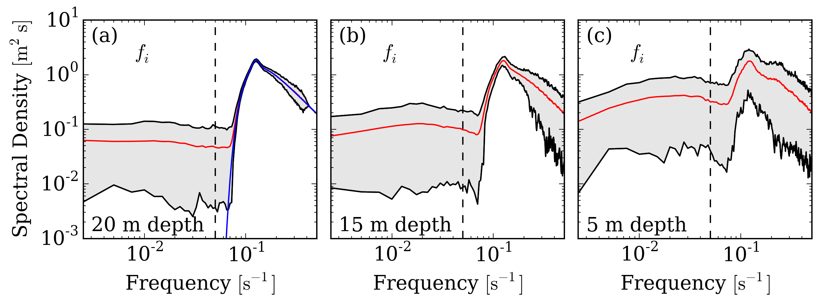
Figure 1: Spectra for in 10 m (a), 15 m (b), and 5 m (c) water depth. From 20 m water depth (a) to 5 m water depth (c), the spectral density increases an order of magnitude in the infragravity frequency band, $f_{i}$. The blue line in (a) refers to input spectrum at the offshore boundary of the computational domain on which the realizations are based. The red line in (a), (b) and (c) represents the average over the hundred realizations, while the grey area defines the envelope.

The maximum spectral density in the infragravity band increases about an order of magnitude as the waves travel from deeper into shallower water. In this particular example, the ratio of infragravity energy to the total energy

$$\widetilde{E}(h)=\dfrac{\sum_{f_{j}<0.05}S_{j}(h)}{\sum_{j}S_{j}(h)}$$ (8)

(where $S_{j}$ is given by Eq. 5) increases from $\widetilde{E}(20\ \text{m})=5.6\times 10^{-4}$ to $\widetilde{E}(15\ \text{m})=2.3\times 10^{-3}$, and $\widetilde{E}(5\ \text{m})=2.6\times 10^{-2}$; the relative spectral content of infragravity energy increases approximately 200 times from 20 m to 5 m water depth.

Figure 2 shows TRIADS simulations of the shoaling evolution of the infragravity energy content $\widetilde{E}$ as a function of water depth for all wave conditions and slopes examined. In general, the energy content increases with increasing significant wave heights and increasing peak periods at all water depths. The increase of the infragravity energy content is stronger for smaller slopes, due to the increased spatial scale over which nonlinear interaction is active.

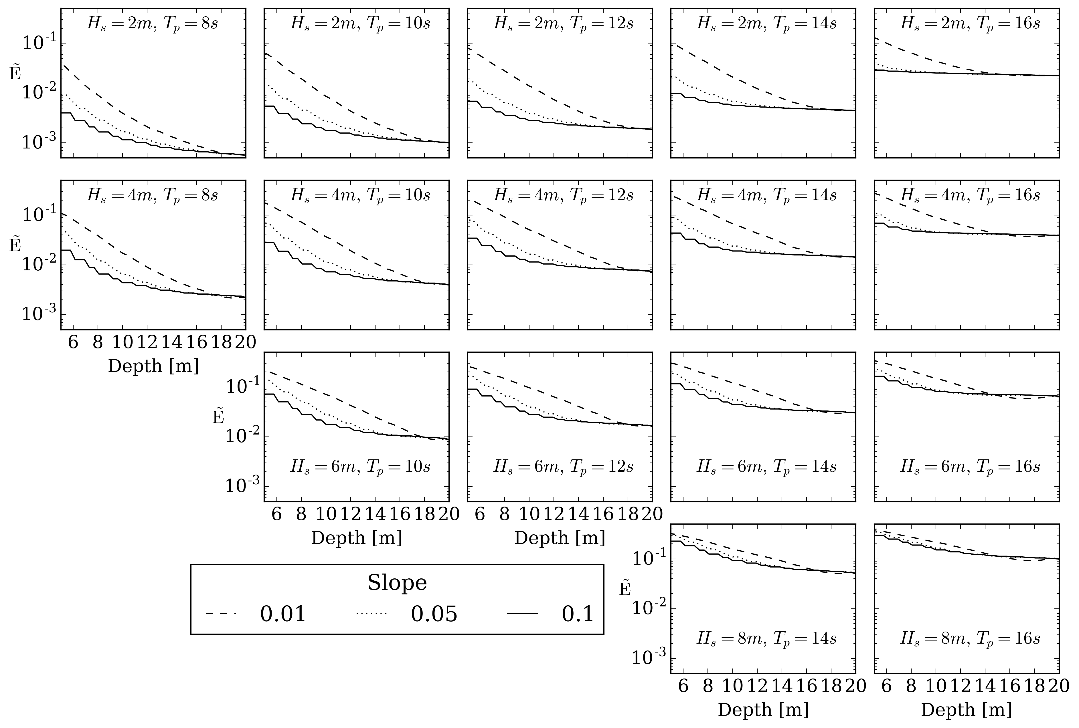
Figure 2: Energy ratio, $\widetilde{E}$, as a function of water depth. The lines in each subplot represent the different slope, and the subplots represent different wave conditions.

Note that estimates of the infragravity energy content are based on spectral quantities (i.e., ensemble-averaged values, Eq. 5, red line in Fig. 1). While the increase in the mean infragravity energy content for $s=0.1$ is the smallest in our tests, it is possible that a small number of realizations will exceed the mean increase corresponding to smallest slope ($s=0.01$). Because individual realizations can exhibit significant deviations from the mean, a significant number of realizations can cause situations at which a boulder can be dislodged, while mean conditions will not or vice versa. Therefore, it is necessary to consider individual realizations to calculate the time series of the velocity that governs the dislodgement of boulders.

3.2 Boulder Dislodgement

In order to find the realizations that for a given wave condition and slope are able to dislodge boulders, time series of the horizontal velocity need the calculated from the individual spectra. Figure 3 depicts time series of the horizontal velocity calculated with Eq. 7 for three of the one hundred realizations. From the longer times in Fig. 3a-c, we can see that the waves generally experience an increase from deep to shallower water. Aside from the increase in significant wave height, we can also see that the time series in deeper water has fewer spikes that are much larger than the majority of wave crests. The number of these outliers increases as well from deep to shallower water.

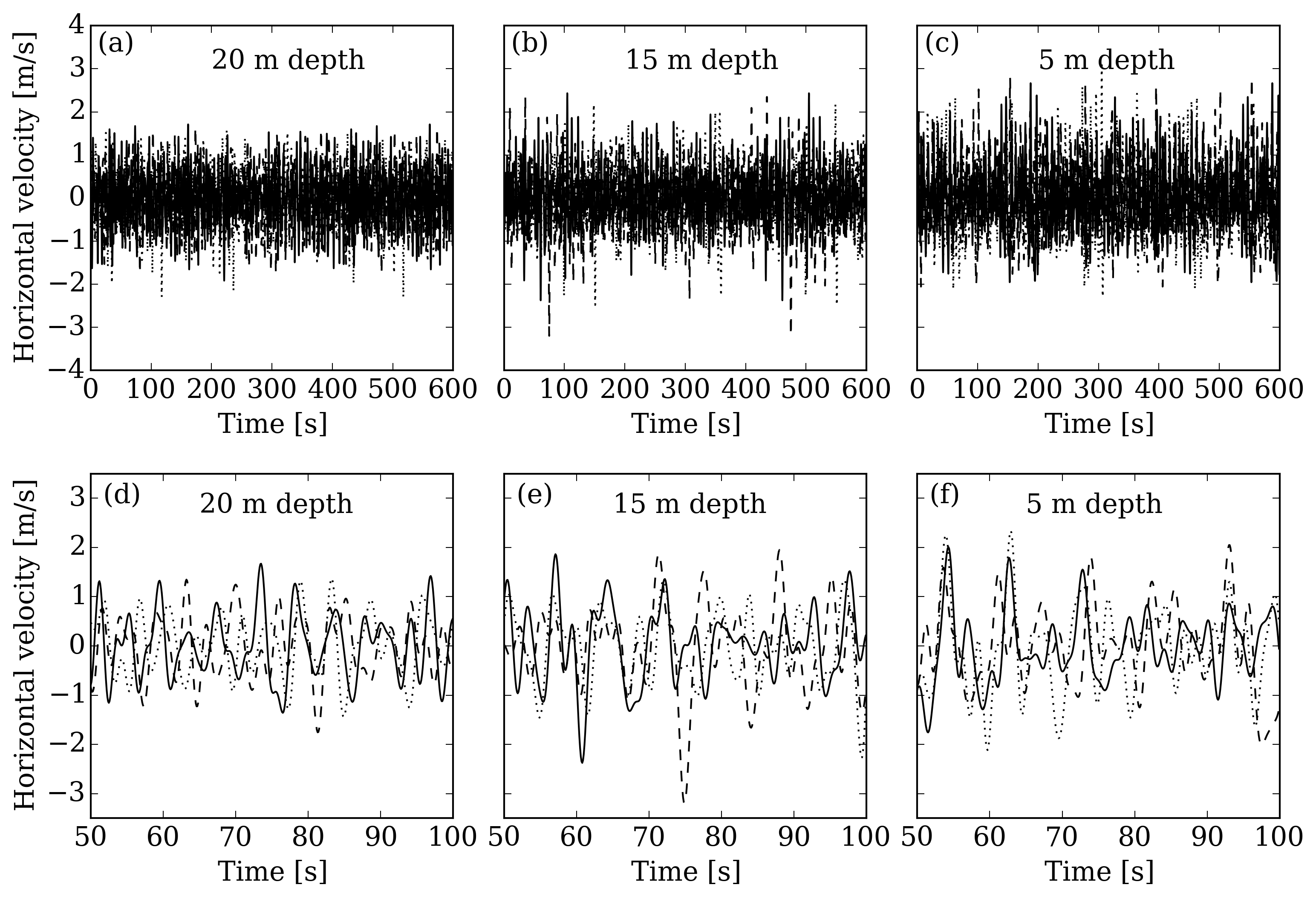
Figure 3: Time series of the horizontal velocity inverted from the spectra for the three randomly chosen realization for the $600s$ (a-c) and from 50 to 100 s (d-f).

The actual wave forms are shown in Fig. 3d-f in time series that only cover 50 seconds instead of 600 seconds (Fig. 3a-c). In all three plots, the superposition of different frequency components leads to complicated velocity time series. We can discern an increase in significant wave height from deeper to shallower water, but what can also be recognized is the increasing asymmetry between the wave crest and trough, which is an effect of the shoaling process. It is also important to note that the qualitative difference between the individual time series increases significantly from deep to shallower water depth. Therefore, a larger variability in the boulder dislodgement frequency can be expected in shallower water. This is a direct result of nonlinear processes acting on the wave during the shoaling process.

Figure 4 shows the dislodgement frequency $D$ as a function of boulder mass for a peak period of 16 seconds, 6 meters in significant wave height, and a roughness of 0.5 of the boulder radius. As expected, we can see that for smaller masses the number of realizations that are able to dislodge boulders is larger than for bigger masses. For example, a dislodgement frequency of larger than 95 is occurs for masses smaller than about $m_{1}=1.4$ tons; for $D=75$, the mass is $2.7t$; for $D=50$, the mass is about $4.6t$; and for $D=25$, the mass is $8.1t$.

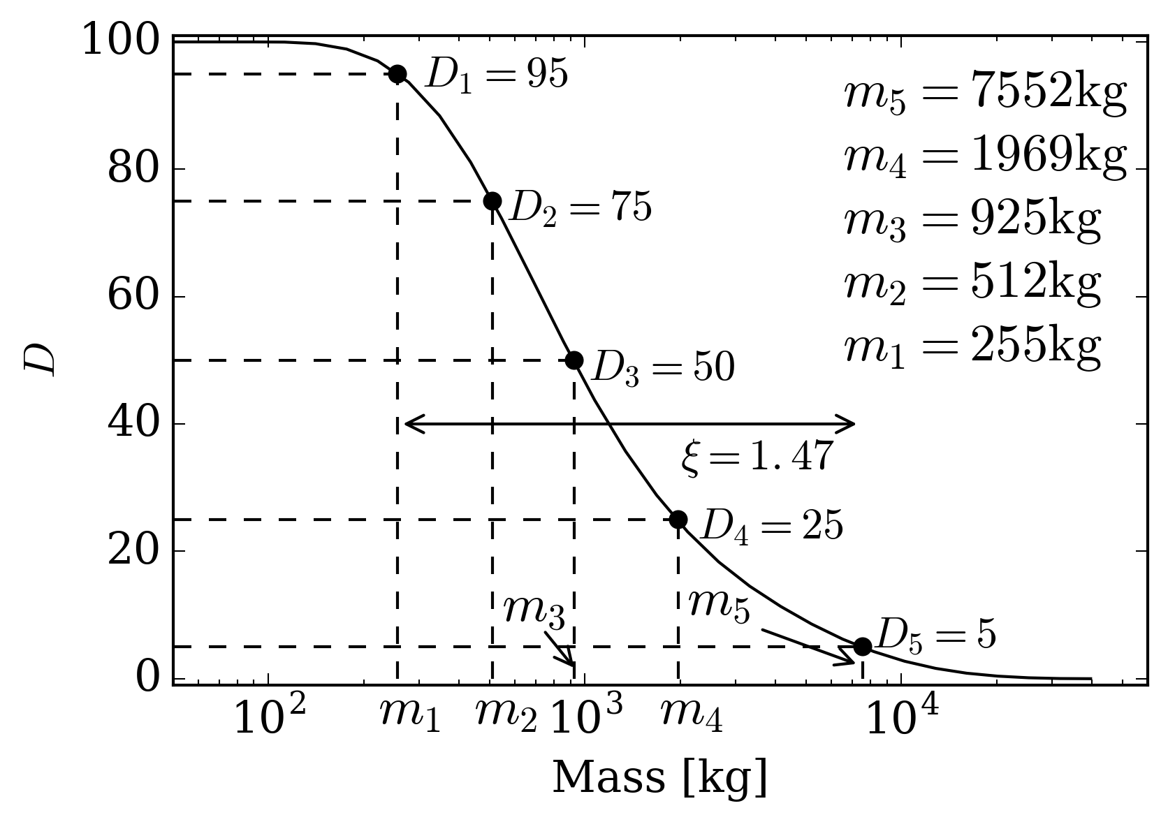
Figure 4: Frequency of dislodgement, $D$ as a function of boulder mass for a peak wave period of $14s$, a significant wave height of $6m$, and roughness of 0.5 the boulder radius.

Figure 5 depicts the frequency of dislodgement for significant wave height, peak periods, slopes, a range of masses and roughnesses. The roughness in all subplots varies from 0.1 to 1.0, and mass varies from about $1kg$ to about $40t$. The different panes in the subplots, marked with $\alpha_{1}$, $\alpha_{2}$ and $\alpha_{3}$, represent the slopes $\alpha_{1}=0.01$, $\alpha_{2}=0.05$, and $\alpha_{3}=0.1$. The different rows indicate an increase of the significant wave height from $2m$ to $8m$, and the wave peak period increases from $8s$ to $16s$ in the different columns. Employing a $\delta=0.5$ to look at the data, we see that only the steepest slope ($\alpha_{3}$) for the condition $H_{s}=2m$, $T_{p}=8s$ is able to have a frequency of dislodgement that is larger than $D=50$. For a significant wave height of $H_{s}=4m$, the mass at which $D=50$ (assuming $\delta=0.5$) increases from about $4kg$ for $T_{p}=8s$ to about $100kg$ for a peak period of $16s$ independent of the slope. For larger significant amplitudes ($H_{s}=6m$ and $H_{s}=8m$), differences for the different slopes are significant. For example for $H_{s}=8m$ and $T_{p}=16s$, the mass for $D=50$ and $\alpha_{1}$ is about $105kg$, for $\alpha_{2}$ the mass is about $900kg$, and for $\alpha_{3}$ the mass is about $2000kg$.

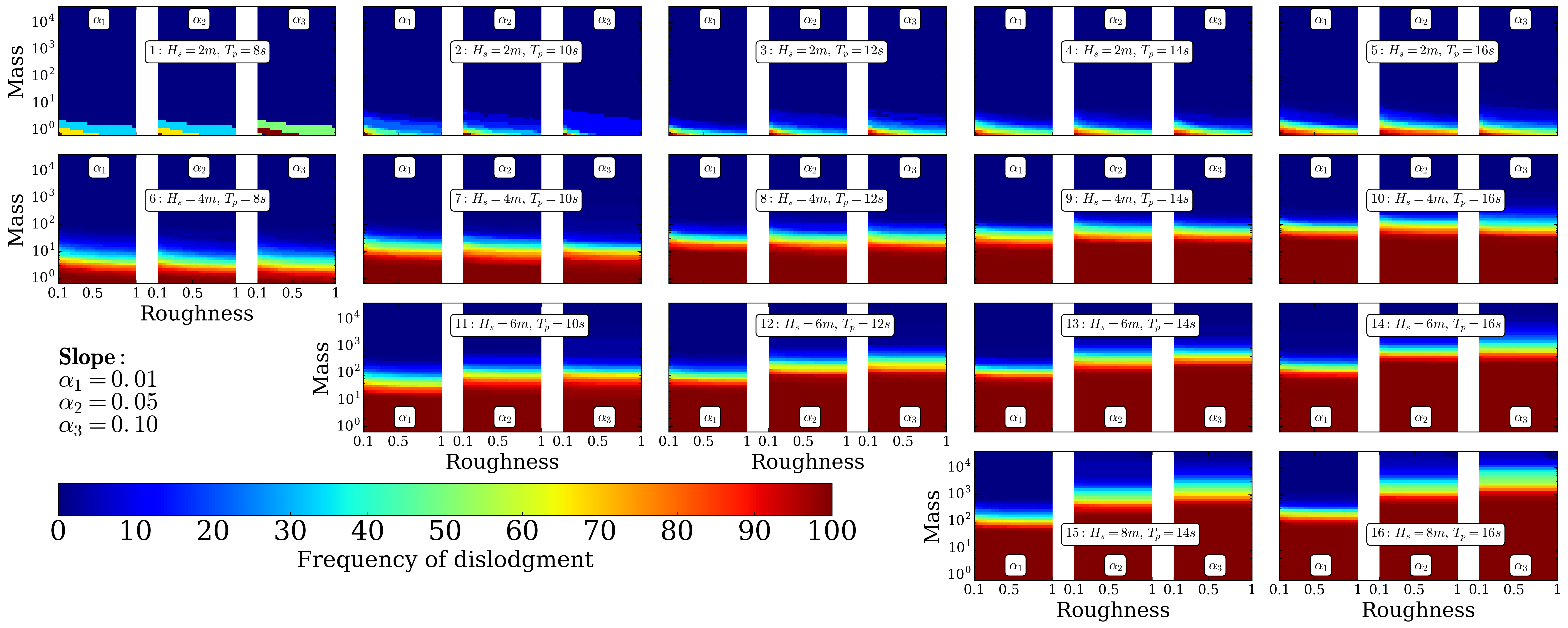
Figure 5: Dislodgement frequency, $D$ as a function of boulder mass for all wave conditions, roughnesses, and slopes.

It is not only important to determine at which masses certain dislodgement frequencies $D$ occur, but also over which mass range an increase from low to high values of $D$ takes place. It should be noted that for the different wave conditions this mass range over which the transition from low to high values of $D$ occurs will take place in the single digit kilogram values to several tons. To eliminate the bias introduced by the wide range of order of magnitude, we define the log-scale difference $\xi$ with $\xi=\log_{10}\left(m_{(\textrm{low}D)}[m_{(\textrm{high}D)}]^{-1}\right)$ in which $m_{(\textrm{low}D)}$ represents the mass with low and $m_{(\textrm{high}D)}$ denotes the mass for a high value of $D$. An example is shown in Fig. 4 in which the log-scale difference between $D=5$ and $D=95$ is calculated to be $\xi=1.47$. Tab 1 contains the log-scale differences for different wave conditions. It is interesting to note that the log-scale difference more than doubles for the different slope angles for larger significant wave heights and longer peak periods and remains more or less constant for small waves and shorter peak periods.

Table 1: Selected wave conditions and their respective log-scale differences, $\xi$, for the different slopes $\alpha_{1}$, $\alpha_{2}$, and $\alpha_{3}$

Wave Condition	Slope	$\xi$
6: $H_{s}=4m$, $T_{s}=8s$	$\alpha_{1}$	1.27
	$\alpha_{2}$	1.27
	$\alpha_{3}$	1.27
9: $H_{s}=4m$, $T_{s}=14s$	$\alpha_{1}$	0.88
	$\alpha_{2}$	0.98
	$\alpha_{3}$	0.88
12: $H_{s}=6m,\,T_{s}=12s$	$\alpha_{1}$	0.98
	$\alpha_{2}$	0.98
	$\alpha_{3}$	1.08
14: $H_{s}=6m,\,T_{s}=16s$	$\alpha_{1}$	0.88
	$\alpha_{2}$	1.08
	$\alpha_{3}$	1.47
16: $H_{s}=8m,\,T_{s}=16s$	$\alpha_{1}$	0.78
	$\alpha_{2}$	1.57
	$\alpha_{3}$	1.67

4 Discussion

As waves propagate from deeper into shallower water, wave-wave interaction transfers energy toward lower and higher frequencies of the spectrum. The latter causes a modification of the wave shape, for example, by increasing the skewness and asymmetry of waves in shallower water (Fig. 3). Transferring wave energy into higher frequencies results into the generation of infragravity waves (Fig. 1). While for all simulated wave conditions and slopes, the increase in infragravity wave energy in shallower water is apparent, the smallest slope exhibits the most significant increase (Fig. 2). This observation can be ascribed to fact that a milder slope allows the waves to nonlinearly interact with each for longer and over a farther distances. The generation of infragravity waves has profound consequences for the individual realizations of the velocity time series needed in the boulder dislodgement model (Fig. 3). As to whether a specific realization can dislodge a boulder of certain mass depends on the specific wave-wave interactions that developed within the time history of the wave propagation. This fact results in the observation that from the same initial wave characteristics one realization is and another realization is not capable of dislodging a boulder of certain mass. How many realizations of a certain initial wave characteristics are able to dislodge a boulder are collected in the frequency of dislodgement. Figures 4 and 5 show the frequency of dislodgement depends on the magnitude of the initial wave characteristics, mass and slope. Obviously, larger waves can dislodge heavier boulders, but it also seems that a smaller slopes cause for heavier boulders to be dislodged more easily that on steeper slopes, which seems to be linked to the aforementioned more significant rise in infragravity energy. Another interesting observation is that the log-scale difference between high and low number of the frequency of dislodgement shows significant diversity for larger initial waves and seems to be much larger for smaller slopes. A simple analysis of the data presented in Fig. 5 reveals that the significant wave height and offshore peak period are proportional to boulder mass and slope angle in a nonlinear fashion, namely $H_{s}\propto(m^{2/3},\alpha^{-2})$ and $T_{p}\propto(m^{1/3},\alpha^{-1})$. This is an interesting results because it goes beyond of what the methods proposed by Nott (2003), Benner et al. (2010), and Nandasena et al. (2011b) are able to predict. More simulations with more offshore wave conditions are needed to establish are robust analysis on how the significant wave height and peak period are related to the roughness in front of the boulder. However, it can be expected that the relationship between significant wave height and peak period, and roughness is nonlinear as well.

5 Conclusion

In this contribution, we coupled the model TRIADS (Sheremet et al., 2016, and references therein) with the boulder-dislodgement model from Weiss and Diplas (2015). Because TRIADS is a nonlinear wave model, it allows the transfer of wave energy across frequencies, which is an important feature observed in coastal waves and was not considered in previously published models of boulder dislodgement during storms. Furthermore, TRIADS describes the evolution of directional triads (as proposed by Agnon and Sheremet, 1997) based on one hundred different initial phases of the same initial spectrum, making it possible to move from a simple framework in which one particular wave is responsible for the dislodgement of one particular boulder mass toward a ensemble approach that reflects the physical and mathematical complexities more realistically. While this stochastic framework is not fully developed in this contribution, we argue that the definition of the frequency of dislodgement is a pivotal intermediate step.

The results of our parameter study match intuitively and quantitatively well with previously published models. Our results also highlight the importance of the environmental parameters, such as slope on which the boulder is resting and the roughness elements in the direction of dislodgement, as long with the boulder mass and characteristics of the waves. For more details on the influence of roughness and slope, see Nott (2003) and Weiss and Diplas (2015). The environmental parameters are difficult, if not impossible, to observe in the field, but we think that the frequency of dislodgement (and later the stochastic framework) will help to, at least, qualitatively assess the uncertainty arising from this shortcoming. Based on the wealth of information contained in Fig. 5, we argue that it is possible and necessary to derive a new boulder dislodgement equation that not only includes boulder mass, roughness in front of the boulder and slope angle, but also frequency of dislodgement. Inverting both components of the wave characteristics is not trivial because $H_{s}$ and $T_{p}$ are both unknowns and there are nonlinear relationships to boulder mass and slope.

In summary, the theoretical consequences of our approach, i.e., the dislodgement frequency and considering waves as a random process, allow us to extend our thinking framework considerably toward a more realistic situation in which the wave spectrum changes its shape depending on water depth and wave-wave interaction and boulder dislodgement is governed not only by the amplitude of the passing waves, but also how long sum of the forces is larger than zero. Through our simulations, it becomes evident that a nonlinear treatment of the waves is pivotal because the nonlinear deformation of the wave shape can generate forces that can be both significantly stronger or weaker and act longer or shorter than those generated by a linear wave with same spectral density distribution. Once there is more information on how the peak period and significant wave height are impacted by the roughness in front of boulder, the ways is paved to derive a new formula for boulder dislodgement based on the frequency of dislodgement. However, no matter the form this new formula will have, the nonlinear relationships between the inverted values of offshore significant wave height and peak period, and variables, such as mass, roughness and slope, the collected data in the field, which are the basis for the inversion, need to be known much more accurately. This is difficult to achieve, introducing, therefore, unwelcome uncertainty. Yet such inversions are extremely important to estimate the hazard coming from storms to improve mitigation efforts. We argue, that a stochastic framework should be able to address the increased uncertainty. In the end, it remains to be seen if a stochastic approach can truly achieve this. Our results, however, indicate that a stochastic approach will be successful.

References

References

- Agnon and Sheremet (1997) Agnon, Y., Sheremet, A., 1997. Stochastic nonlinear shoaling of directional spectra. Journal of Fluid Mechanics 345, 79–99.
- Benner et al. (2010) Benner, R., Browne, T., Brückner, H., Kelletat, D., Scheffers, A., 2010. Boulder transport by waves: progress in physical modelling. Zeitschrift für Geomorphologie, 127–146.
- Buckley et al. (2012) Buckley, M. L., Wei, Y., Jaffe, B. E., Watt, S., 2012. Inverse modeling of velocities and inferred cause of overwash that emplaced inland fields of boulders at Anegada, British Virgin Islands. Natural Hazards 63 (1), 133–149.
- Cash and Carp (1990) Cash, J. R., Carp, A. H., 1990. A variable Runge-Kutta method for initial value problems with rapidly varying right-hand side. {ACM} Trans. Math. Softw. 16, 201–220.
- Davis J.R. et al. (2014) Davis J.R., A. S., M. Tian, Saxena, S., 2014. A Numerical Implementation of a Nonlinear Mild Slope Model for Shoaling Directional Waves. J. Mar. Sci. Eng. 2, 140–158.
- Fehlberg (1969) Fehlberg, E., 1969. Low-order classical Runge-Kutta formulas and their application to some heat transfer problems. Tech. Rep. Report 315, NASA.
- Hasselmann K. et al. (1973) Hasselmann K., T., Barnett, P., Bouws, E., Carlson, H., Cartwright, D. E., Enke, K., Ewing, J. A., Gienapp, H., Hasselmann, D. E., Kruseman, P., Meerburg, A., Muller, P., Olbers, D. J., Richter, K., Sell, W., H., W., 1973. Measurements of Wind-Wave Growth and Swell Decay during the Joint North Sea Wave Project (JONSWAP). Tech. Rep. UDO 551.466.31; ANE German Bight, Deutsches Hydrographisches Institut, Hamburg.
- Herbers et al. (1994) Herbers, T. H. C., Elgar, S., Guza, R. T., Herbers, T. H. C., Elgar, S., Guza, R. T., 1994. Infragravity-Frequency (0.005–0.05 Hz) Motions on the Shelf. Part I: Forced Waves. http://dx.doi.org/10.1175/1520-0485(1994)024¡0917:IFHMOT¿2.0.CO;2.
- Herbers et al. (1995) Herbers, T. H. C., Elgar, S., Guza, R. T., O’Reilly, W. C., Herbers, T. H. C., Elgar, S., Guza, R. T., O’Reilly, W. C., 1995. Infragravity-Frequency (0.005–0.05 Hz) Motions on the Shelf. Part II: Free Waves. http://dx.doi.org/10.1175/1520-0485(1995)025¡1063:IFHMOT¿2.0.CO;2.
- Kennedy et al. (2016) Kennedy, A. B., Mori, N., Zhang, Y., Yasuda, T., Chen, S.-E., Tajima, Y.and Pecor, W., Toride, K., 2016. Observations and Modeling of Coastal Boulder Transport and Loading During Super Typhoon Haiyan. Coastal Engineering Journal 58 (01), 1640004.
- Krumbein and Aberdeen (1937) Krumbein, W. C., Aberdeen, E., 1937. The Sediments of Barataria Bay. Journal of Sedimentary Pretrology 7 (1), 3–17.
-
Langtangen and Wang (2013)
Langtangen, H. P., Wang, L., 2013. The Odespy package.
URL https://github.com/hplgit/odespy - Nandasena et al. (2011a) Nandasena, N. A. K., Paris, R., Tanaka, N., 2011a. Numerical assessment of boulder transport by the 2004 Indian ocean tsunami in Lhok Nga, West Banda Aceh (Sumatra, Indonesia). Computers & Geosciences 37 (9), 1391–1399.
- Nandasena et al. (2011b) Nandasena, N. A. K., Paris, R., Tanaka, N., 2011b. Reassessment of hydrodynamic equations to initiate boulder transport by high-energy events (storms, tsunamis). Marine Geology 281, 70–84.
- Nott (2003) Nott, J., 2003. Waves, coastal boulders and the importance of pre-transport setting.
- Sheremet et al. (2016) Sheremet, A., Davis, J. R., Tian, M., Hanson, J. L., Hathaway, K. K., 2016. TRIADS: a phase-resolving model for nonlinear shoaling of directional wave spectra.
-
Sheremet et al. (2002)
Sheremet, A., Guza, R. T., Elgar, S., Herbers, T. H. C., 2002. Observations of
nearshore infragravity waves: Seaward and shoreward propagating components.
Journal of Geophysical Research 107 (C8), 3095.
URL http://doi.wiley.com/10.1029/2001JC000970 - Weiss and Diplas (2015) Weiss, R., Diplas, P., 2015. Untangling boulder dislodgment in storms and tsunamis: Iis it possible with simple theories?