Online Learning for Distribution-Free Prediction

Abstract

We develop an online learning method for prediction, which is important in problems with large and/or streaming data sets. We formulate the learning approach using a covariance-fitting methodology, and show that the resulting predictor has desirable computational and distribution-free properties: It is implemented online with a runtime that scales linearly in the number of samples; has a constant memory requirement; avoids local minima problems; and prunes away redundant feature dimensions without relying on restrictive assumptions on the data distribution. In conjunction with the split conformal approach, it also produces distribution-free prediction confidence intervals in a computationally efficient manner. The method is demonstrated on both real and synthetic datasets.

1 Introduction

Prediction is a classical problem in statistics, signal processing, system identification and machine learning [1, 2, 3, 4]. The prediction of stochastic processes was pioneered in the temporal and spatial domains, cf. [5, 6, 7, 8], but the fundamental ideas were generalized to arbitrary domains. In general, the problem can be formulated as predicting the output of a process, $y$, for a given input test point $\mathbf{x}$ after observing a dataset of input-output pairs

$$\mathcal{D}=\bigl{\{}(\mathbf{x}_{1},y_{1}),\>\dots,\>(\mathbf{x}_{n},y_{n})\bigr{\}}.$$

In this paper, we are interested in learning predictor functions $\widehat{y}(\mathbf{x})$ in scenarios where $n$ is very large or is increasing. We consider two common classes of predictors:

1. The first class consists of predictors in linear regression (Lr) form. That is, given a regressor function $\boldsymbol{\phi}(\mathbf{x})$, the predictor $\widehat{y}(\mathbf{x})$ is expressed as a linear combination of its elements. This class includes ridge regression, Lasso, and elastic net [9, 10, 11]. The regressor $\boldsymbol{\phi}(\mathbf{x})$ can be understood as a set of input features and a standard choice for it is simply $\mathbf{x}$.

2. The second class comprises predictors in linear combiner (Lc) form. That is, the predictor $\widehat{y}(\mathbf{x})$ is expressed as a linear combination of all observed samples $\{y_{i}\}$, using a model of the process. This class includes kernel smoothing, Gaussian process regression, and local polynomial regression [12, 13, 14, 15, 16]. A standard model choice is a squared-exponential kernel or covariance function for $y$.

The weights in the Lr and Lc classes are denoted $\mathbf{w}$ and $\boldsymbol{\lambda}$, respectively. For a given prediction method in either class, the weights are functions of the data $\mathcal{D}$. The set of possible weights is large and must be constrained in a balanced manner to avoid a high variance and bias of $\widehat{y}(\mathbf{x})$, which correspond to overfitting and underfitting, respectively.

In most prediction methods, the constraints on the set of weights are controlled using a hyperparameter, which we denote $\boldsymbol{\theta}$ and which is learned from data. There exist several methods for doing so, including cross-validation, maximum likelihood, and weighted least-squares [1, 17, 18]. These learning methods are, however, nonconvex and not readily scalable to large $n$, which is the target case of this paper. Moreover, in the process of quantifying the prediction uncertainty, using e.g. the bootstrap [19] or conformal approaches [20, 21], the learning methods compound the complexity and render such uncertainty quantification intractable for large $n$.

In this paper, we consider a class of predictors $\widehat{y}(\mathbf{x};\boldsymbol{\theta})$ that can equivalently be expressed in either linear regression or combiner form. In this class, $\boldsymbol{\theta}$ constrains the weights for each dimension of $\boldsymbol{\phi}(\mathbf{x})$ individually. Thus irrelevant features can be suppressed and overfitting mitigated [22, 23, 4]. To learn the hyperparameters $\boldsymbol{\theta}$, we employ a covariance-fitting methodology [18, 24, 25] by generalizing a fitting criterion used in [26, 27, 28]. We extend this learning approach to a predictive setting, which results in a predictor with the following attributes:

• computable online in linear runtime,

• implementable with constant memory,

• does not suffer from local minima problems,

• enables tractable distribution-free confidence intervals,

• prunes away irrelevant feature dimensions.

These facts render the predictor particularly suitable for scenarios with large and/or growing number of data points. It can be viewed as an online, distribution-free alternative to the automatic relevance determination approach [22, 23, 4]. Our contributions include generalizing the covariance-fitting methodology to non-zero mean structures, providing connections between linear regression and combiner-type predictors, and an analysis of prediction performance when the distributional form of the data is unknown.

The remainder of the paper is organized as follows. In Section 2, we introduce the problem of learning hyperparameters. In Section 3, we highlight desirable constraints on the weights in an Lr setting, whereas Section 4 highlights these constraints in an Lc setting. The hyperparameters constrain the weights in different ways in each setting. In Section 5, the covariance-fitting based learning method is introduced and applied to an Lc predictor. The resulting computational and distribution-free properties are derived. Finally, in Section 6, the proposed online learning approach is compared with the offline cross-validation approach on a series of real and synthetic datasets.

Remark 1.

In the interest of reproducible research, we have made the code for the proposed method available at https://github.com/dzachariah/online-learning. $\Diamond$

Notation: $\odot$ is the elementwise Hadamard product. The operation $\operatorname{col}\{\mathbf{x}_{1},\dots,\mathbf{x}_{n}\}$ stacks all $\mathbf{x}_{i}$ into a single column vector, while $[\mathbf{X}]_{i}$ denotes the $i$th column of $\mathbf{X}$. The sample mean is written as $\widehat{\text{E}}[\mathbf{x}_{i}]=n^{-1}\sum^{n}_{i=1}\mathbf{x}_{i}$. The number of nonzero elements in a vector is denoted as $\|\mathbf{x}\|_{0}$. The Kronecker delta is denoted $\delta(\mathbf{x},\mathbf{y})$.

Abbreviations: Independent and identically distributed (i.i.d.).

2 Learning problem

Let $\widehat{y}(\mathbf{x};\boldsymbol{\theta})$ denote a predictor with hyperparameters $\boldsymbol{\theta}$. For linear regression and combiner-type predictors, the choice of $\boldsymbol{\theta}$ constrains the set of weights. For any input-output pair $(\mathbf{x},y)$, the risk of the predictor is taken to be the mean-squared error [29]

$$\mathcal{R}\triangleq\operatorname{E}\left[\left|y-\widehat{y}(\mathbf{x};\boldsymbol{\theta})\right|^{2}\right].$$ (1)

The optimal choice of $\boldsymbol{\theta}$ is therefore the hyperparameter that minimizes the unknown risk. A common distribution-free learning approach is cross-validation, which estimates the risk for a fixed choice of $\boldsymbol{\theta}$. The risk estimate is formed by first dividing the training data into $K$ subsets and then predicting the output in one subset using data from the remaining $K-1$ subsets[1, ch. 7]:

$$\widehat{\mathcal{R}}(\boldsymbol{\theta})\>=\>\sum^{K}_{k=1}\frac{n_{k}}{n}\>\widehat{\text{E}}\left[\left|y_{i}-\widehat{y}_{\neg k}(\mathbf{x}_{i};\boldsymbol{\theta})\right|^{2}\right],$$ (2)

where $n_{k}$ is the number of samples in subset $k$ and $\widehat{y}_{\neg k}(\mathbf{x};\boldsymbol{\theta})$ denotes the predictor using training data from all subsets except $k$. In this approach, the hyperparameter is learned by finding $\widehat{\boldsymbol{\theta}}$ that minimizes $\widehat{\mathcal{R}}(\boldsymbol{\theta})$. For one-dimensional hyperparameters, a numerical search for the minimum of (2) is feasible when $K$ is small; otherwise it may well be impractical.

An alternative learning approach is to assume that the distribution of $(\mathbf{x},y)$ belongs to a family that is parameterized by $\boldsymbol{\theta}$. Then the hyperparameter can be learned by fitting a covariance model of the data to the empirical moments of the training data, cf. [18]. If additional assumptions are made about the distributional form, it is possible to formulate a complete probabilistic model of the data and learn $\boldsymbol{\theta}$ using the asymptotically efficient maximum likelihood approach, cf. [30, 17].

The aforementioned statistical learning methods are, however, in general nonconvex and may therefore give rise to multiple minima problems [31, 32]. This becomes problematic when $\boldsymbol{\theta}$ is multidimensional as the methods may require a careful choice of initialization and numerical search techniques [33, ch. 5]. In addition, the distributional assumptions employed in the maximum likelihood approach may lack robustness to model misspecifications [34].

More importantly for the data scenarios considered in this paper, these learning methods cannot readily be implemented online. That is, for a given dataset, the computational complexity of learning $\boldsymbol{\theta}$ does not scale well with $n$ and the process must be repeated each time $n$ increases. Consequently, for each new $\widehat{\boldsymbol{\theta}}$, the predictor function $\widehat{y}(\mathbf{x};\widehat{\boldsymbol{\theta}})$ must be computed afresh.

Our main goal is to develop a learning approach that is implementable online, obviates local minima problems, and has desirable distribution-free properties. Before we introduce the proposed learning approach, we introduce the hyperparameters in the context of Lr and Lc predictors, respectively.

3 Linear regression predictor

Lr predictors are written in the following form

$$\boxed{\widehat{y}(\mathbf{x})=\boldsymbol{\phi}^{\top}(\mathbf{x})\mathbf{w},}$$ (3)

where $\boldsymbol{\phi}(\mathbf{x})$ is a $p$-dimensional regression function and $\mathbf{w}$ are weights. The empirical risk of a predictor can then be written as

$$R(\mathbf{w})\triangleq\widehat{\text{E}}\left[|y_{i}-\boldsymbol{\phi}^{\top}(\mathbf{x}_{i})\mathbf{w}|^{2}\right].$$ (4)

When the empirical risk is minimized under a constraint on $\mathbf{w}$, irrelevant dimensions of $\boldsymbol{\phi}(\mathbf{x})$ can be suppressed which mitigates overfitting [1, 35]. For notational convenience we write the regressor matrix as

$$\boldsymbol{\Phi}\triangleq\begin{bmatrix}\boldsymbol{\phi}^{\top}(\mathbf{x}_{1})\\ \vdots\\ \boldsymbol{\phi}^{\top}(\mathbf{x}_{n})\end{bmatrix}=\begin{bmatrix}\widetilde{\boldsymbol{\phi}}_{1}&\cdots&\widetilde{\boldsymbol{\phi}}_{p}\end{bmatrix},$$

where $\widetilde{\boldsymbol{\phi}}_{j}$ denotes the $j$th column.

When $p$ is large, we would ideally like to find a subset of at most $k\ll p$ relevant dimensions [1, 36, 37, 38]. We may then define the optimal weights as

$$\begin{split}\mathbf{w}_{\star}\>&\triangleq\>\operatorname*{arg\,min}_{\mathbf{w}\>:\>\|\mathbf{w}\|_{0}\leq k}\;R(\mathbf{w}).\end{split}$$ (5)

Let $\widehat{y}_{\star}(\mathbf{x})=\boldsymbol{\phi}^{\top}(\mathbf{x})\mathbf{w}_{\star}$ denote corresponding optimal Lr predictor. This sparse predictor does not rely on any assumptions on the data, and is therefore robust to model misspecifications. We collect the prediction errors of the training data in the vector

$$\boldsymbol{\varepsilon}=\operatorname{col}\{\varepsilon_{1},\dots,\varepsilon_{n}\},$$

where $\varepsilon_{i}=y_{i}-\widehat{y}_{\star}(\mathbf{x}_{i})$. In the subsequent analysis, we also make use of

$$\varepsilon_{\star}\;\triangleq\;\max_{1\leq j\leq p}\;\left|\boldsymbol{\varepsilon}^{\top}\widetilde{\boldsymbol{\phi}}_{j}\right|.$$ (6)

Solving (5) is a computationally intractable problem, even for moderately sized $p$. Thus $\widehat{y}_{\star}(\mathbf{x})$ will be taken as a reference against which any alternative $\widehat{y}(\mathbf{x})$ can be compared by defining the prediction divergence [39]:

$$\begin{split}\Delta_{\star}\>\triangleq\>\widehat{\text{E}}\left[\bigl{|}\widehat{y}(\mathbf{x}_{i})-\widehat{y}_{\star}(\mathbf{x}_{i})\bigr{|}^{2}\right].\end{split}$$ (7)

A tractable convex relaxation of the problem in (5) is the $\ell_{1}$-regularized Lasso method [10], as defined by

$$\begin{split}\widehat{\mathbf{w}}\>&=\>\operatorname*{arg\,min}_{\mathbf{w}}\;R(\mathbf{w})+\theta\|\mathbf{w}\|_{1},\end{split}$$ (8)

where $\theta\geq 0$ is a hyperparameter that shrinks all weights toward zero in a sparsifying fashion. This Lr predictor has desirable risk-minimizing properties and can be computed online in linear runtime for any fixed $\theta$ [40, 41]. The corresponding divergence can be bounded per the following result.

Result 1.

If the hyperparameter satisfies

$$\theta\geq\frac{2\varepsilon_{\star}}{n},$$ (9)

then the divergence of the Lasso-based predictor $\widehat{y}(\mathbf{x})$ from the optimal sparse predictor $\widehat{y}_{\star}(\mathbf{x})$ is bounded by

$$\Delta_{\star}\>\leq\>2\theta\|\mathbf{w}_{\star}\|_{1}.$$ (10)

Proof.

See Appendix A.1 ∎

If the hyperparameter $\theta$ in (8) satisfies (9), then (10) ensures that the maximum divergence of Lasso-based predictor from the optimal Lr predictor remains bounded. Then redundant dimensions of $\boldsymbol{\phi}(\mathbf{x})$ are pruned away, which is a desirable property. The hyperparameter $\theta$ in (8) is typically learned offline using (2), which is a limitation for the scenarios of large and/or increasing $n$ considered herein. Moreover, the individual weights in (3) are constrained uniformly in the Lasso approach. To provide a more flexible predictor that constrains the weights individually, we consider an Lc approach next.

Remark 2.

For the special case in which the prediction errors of $\widehat{y}_{\star}(\mathbf{x})$ are i.i.d. zero mean Gaussian with variance $\sigma^{2}$, and the regressors are normalized such that $\|\widetilde{\boldsymbol{\phi}}_{j}\|^{2}\equiv n$, the inequality (9) is satisfied with high probability when $\theta=\sigma\sqrt{(2\ln p+\delta)/n}$ for some positive constant $\delta$, cf. [39]. However, this is an infeasible choice since $\sigma^{2}$ is unknown and must be estimated. $\Diamond$

4 Linear combiner predictor

Lc predictors are written in the following form

$$\boxed{\widehat{y}(\mathbf{x})=\boldsymbol{\lambda}^{\top}(\mathbf{x})\mathbf{y},}$$ (11)

where $\mathbf{y}=\operatorname{col}\{y_{1},\dots,y_{n}\}$ contains the $n$ observed samples and $\boldsymbol{\lambda}$ are weights. Given any $\mathbf{x}$, we will find an unbiased predictor of $y$ that minimizes the conditional risk. That is, we seek the solution to

$$\begin{split}\min_{\boldsymbol{\lambda}}\;\mathcal{R}(\boldsymbol{\lambda}|\mathbf{x}),\quad\text{subject to}\>\operatorname{E}\left[y-\boldsymbol{\lambda}^{\top}\mathbf{y}\>|\>\mathbf{X},\mathbf{x}\right]=0,\end{split}$$ (12)

where

$$\mathcal{R}(\boldsymbol{\lambda}|\mathbf{x})=\operatorname{E}\left[\bigl{|}y-\boldsymbol{\lambda}^{\top}\mathbf{y}\bigr{|}^{2}\>|\>\mathbf{X},\mathbf{x}\right],$$

and $\mathbf{X}$ denotes all inputs in $\mathcal{D}$. The weights $\boldsymbol{\lambda}$ are then constrained by assuming a model of $y$ given $\mathbf{x}$.

Here we specify a simple model that does not rely on the distributional form of $y$ but merely constrains its moments [30]:

• The conditional mean of $y$ is parameterized as

  $$\operatorname{E}[y|\mathbf{x}]=\mathbf{u}^{\top}(\mathbf{x})\mathbf{w}_{0},$$ (13)

  where $\mathbf{u}(\mathbf{x})$ is a given $u\times 1$ function and $\mathbf{w}_{0}$ are unknown coefficents. In the simplest case we have an unknown constant mean, i.e., $\operatorname{E}[y|\mathbf{x}]\equiv w_{0}$, by setting $\mathbf{u}(\mathbf{x})\equiv 1$. Alternatively, one may consider an unknown affine function.

• The conditional covariance function can be expressed as

  $$\begin{split}\operatorname{Cov}[y,y^{\prime}|\mathbf{x},\mathbf{x}^{\prime}]&=\sum^{\infty}_{k=1}\theta_{k}\psi_{k}(\mathbf{x})\psi_{k}(\mathbf{x}^{\prime})+\theta_{0}\delta(\mathbf{x},\mathbf{x}^{\prime})\end{split}$$ (14)

  using Mercer’s theorem [30], where $\psi_{k}(\mathbf{x})$ is given and $\theta_{k}$ are nonnegative parameters. For a stationary process with an isotropic covariance function, we may for instance use the Fourier or Laplace operator basis $\psi_{k}(\mathbf{x})$ [42, 43].

To enable an computationally efficient online implementation, we consider a model with a truncated sum of $q$ terms in (14). We write

$$\boldsymbol{\psi}(\mathbf{x})=\operatorname{col}\{\psi_{1}(\mathbf{x}),\dots,\psi_{q}(\mathbf{x})\}$$

and the hyperparameter as

$$\boldsymbol{\theta}\triangleq\operatorname{col}\{\theta_{0},\theta_{1},\dots,\theta_{q}\},$$

for notational simplicity.

Remark 3.

The model, specified by (13) and (14), is invariant with respect to the distributional properties of the data. It therefore includes commonly assumed distributions, such as Gaussian and Student-t [33, 44]. $\Diamond$

Remark 4.

When $y$ is modelled as a stationary process, the Fourier or Laplace operator basis can be used in (14) to parameterize its power spectral density via $\{\theta_{k}\}$. This can be interpreted as a way to parameterize the smoothness of the process [30]. $\Diamond$

Result 2.

Under model assumptions (13) and (14), the covariance properties of the training data are given by

$$\begin{split}\boldsymbol{\Sigma}&\triangleq\operatorname{Cov}[\mathbf{y}|\mathbf{X}]=\boldsymbol{\Psi}\boldsymbol{\Theta}\boldsymbol{\Psi}^{\top}+\theta_{0}\mathbf{I}_{n}\\ \mathbf{r}(\mathbf{x})&=\operatorname{Cov}[\mathbf{y},y|\mathbf{X},\mathbf{x}]=\boldsymbol{\Psi}\boldsymbol{\Theta}\boldsymbol{\psi}(\mathbf{x}),\end{split}$$ (15)

where

$$\begin{split}\boldsymbol{\Psi}&=\begin{bmatrix}\boldsymbol{\psi}(\mathbf{x}_{1})&\cdots&\boldsymbol{\psi}(\mathbf{x}_{n})\end{bmatrix}^{\top},\\ \boldsymbol{\Theta}&=\operatorname{diag}(\theta_{1},\dots,\theta_{q}).\end{split}$$

Proof.

The result follows from an elementwise application of (14) to the training data:

$$\begin{split}\operatorname{Cov}[y_{i},y_{j}|\mathbf{x}_{i},\mathbf{x}_{j}]&=\sum^{q}_{k=1}\theta_{k}\psi_{k}(\mathbf{x}_{i})\psi_{k}(\mathbf{x}_{j})+\theta_{0}\delta(i,j),\\ \operatorname{Cov}[y_{i},y|\mathbf{x}_{i},\mathbf{x}]&=\sum^{q}_{k=1}\theta_{k}\psi_{k}(\mathbf{x}_{i})\psi_{k}(\mathbf{x}).\\ \end{split}$$

∎

Result 3.

The weights of the optimal Lc predictor $\widehat{y}(\mathbf{x};\boldsymbol{\theta})$ in (11) are given by

$$\begin{split}\boldsymbol{\lambda}(\mathbf{x})&=\boldsymbol{\Sigma}^{-1}\mathbf{U}(\mathbf{U}^{\top}\boldsymbol{\Sigma}^{-1}\mathbf{U})^{\dagger}\mathbf{u}(\mathbf{x})+\boldsymbol{\Sigma}^{-1}\boldsymbol{\Pi}^{\perp}\mathbf{r}(\mathbf{x}),\end{split}$$ (16)

where

$$\mathbf{U}=\begin{bmatrix}\mathbf{u}(\mathbf{x}_{1})&\cdots&\mathbf{u}(\mathbf{x}_{n})\end{bmatrix}^{\top}.$$

and $\boldsymbol{\Pi}^{\perp}$ is a projector onto $\text{span}(\mathbf{U})^{\perp}$.

Proof.

See Appendix B. ∎

Consequently, the hyperparameters in $\boldsymbol{\theta}$ constrain the optimal weights $\boldsymbol{\lambda}$ via the model (13) and (14). If the model were correctly specified, we could in principle search for a risk-minimizing $\boldsymbol{\theta}$. This would, however, be intractable in an online setting.

Next, we show that it is possible to interchange Lc and Lr representations, (11) and (3), of the predictor $\widehat{y}(\mathbf{x};\boldsymbol{\theta})$.

Result 4.

The optimal Lc predictor in (11) and (16) can be written in Lr form

$$\widehat{y}(\mathbf{x};\boldsymbol{\theta})=\boldsymbol{\phi}^{\top}(\mathbf{x})\widehat{\mathbf{w}},$$ (17)

where

$$\boldsymbol{\phi}(\mathbf{x})=\operatorname{col}\{\mathbf{u}(\mathbf{x}),\boldsymbol{\psi}(\mathbf{x})\}$$ (18)

and the $p=u+q$ weights are given by

$$\widehat{\mathbf{w}}=\operatorname*{arg\,min}_{\mathbf{w}}\>R(\mathbf{w})+\frac{\theta_{0}}{n}\|\mathbf{w}\|^{2}_{\mathbf{D}},$$ (19)

where $\mathbf{D}=\operatorname{diag}(\mathbf{0},\boldsymbol{\Theta}^{-1})$.

Proof.

See Appendix C. ∎

Remark 5.

Note that, if we impose $\theta_{1}=\cdots=\theta_{q}\equiv 1$, (19) is equivalent to the ridge regression method [9]. $\Diamond$

Remark 6.

The Lc predictor has an Lr intepretation: when (14) is formed using the Fourier or Laplace operator basis, the corresponding regressor (18) will approximate any isotropic covariance function by varying $\boldsymbol{\theta}$. This includes covariance functions belonging to the important Matérn class, of which the popular squared-exponential function is a special case [30, ch. 6.5]. Cf. [42, 43, 45] for regressor functions $\boldsymbol{\phi}(\mathbf{x})$ with good approximation properties. Similarly, by partitioning an arbitrary regressor $\boldsymbol{\phi}(\mathbf{x})$ into the form (18) yields an Lc interpretation of an Lr predictor. The regressor matrix is then $\boldsymbol{\Phi}=[\mathbf{U}\>\boldsymbol{\Psi}]$. For instance, a standard regressor is the affine function $\boldsymbol{\phi}(\mathbf{x})=\operatorname{col}\{1,\mathbf{x}\}$, which can be interpreted as a constant mean with a covariance function that is quadratic in $\mathbf{x}$. $\Diamond$

The elements of $\boldsymbol{\theta}$ constrain each of the weights (19) individually, unlike the uniform approach in (8). Thus the hyperparameter in the optimal Lc predictor determines the relevance of individual features in $\boldsymbol{\phi}(\mathbf{x})$, similar to the automatic relevance determination framework in [23, 46, 47]. While this enables a more flexible predictor, the $\ell_{2}$-regularization term in (19) does not yield the sparsity property of the Lasso-based predictor. More importantly, the learning approach (2) is intractable when $\boldsymbol{\theta}$ is multidimensional. We show how to get around this issue in the next section.

5 Online learning via covariance fitting

We consider a covariance-fitting approach for learning $\boldsymbol{\theta}$ in the flexible Lc predictor. We show that using the learned hyperparameter results in a predictor with desirable, computational and distribution-free, properties.

The normalized sample covariance matrix of the training data can be written as

$$\begin{split}\widetilde{\mathbf{Z}}&=\frac{(\mathbf{y}-\mathbf{U}\mathbf{w}_{0})(\mathbf{y}-\mathbf{U}\mathbf{w}_{0})^{\top}}{\|\mathbf{y}-\mathbf{U}\mathbf{w}_{0}\|_{2}},\end{split}$$

using the mean structure (13). The assumed covariance structure $\boldsymbol{\Sigma}$ is parameterized by $\boldsymbol{\theta}$ in (15). We seek to fit $\boldsymbol{\Sigma}$ to the sample covariance in the following sense:

$$\begin{split}\boxed{\boldsymbol{\theta}^{\star}=\operatorname*{arg\,min}_{\boldsymbol{\theta}}\quad\bigl{\|}\>\widetilde{\mathbf{Z}}-\boldsymbol{\Sigma}\>\bigr{\|}^{2}_{\boldsymbol{\Sigma}^{-1}},}\end{split}$$ (20)

using a weighted norm that penalizes correlated residuals, cf. [18, 24, 25]. To match the magnitude of the normalized sample covariance we subject the parameters in (20) to the normalization constraint

$$\text{tr}\bigl{\{}\widetilde{\mathbf{Z}}-\boldsymbol{\Sigma}\bigr{\}}=0.$$ (21)

Result 5.

The learning problem defined by (20) is convex in $\boldsymbol{\theta}$ and will therefore not suffer from local minima issues.

Proof.

See Appendix D. ∎

Remark 7.

Eq. (20) is a generalization of the covariance-fitting criterion in [26, 27] to the case of nonzero mean structures of the data. See also [48] for further connections. $\Diamond$

5.1 Properties of the resulting predictor

Using (20) in the Lc predictor from (11) and (16), we obtain the following result:

Result 6.

The Lc predictor with a learned parameter $\boldsymbol{\theta}^{\star}$ has the following Lr form:

$$\widehat{y}(\mathbf{x};\boldsymbol{\theta}^{\star})=\boldsymbol{\phi}^{\top}(\mathbf{x})\widehat{\mathbf{w}}$$ (22)

where

$$\boxed{\widehat{\mathbf{w}}\>=\>\operatorname*{arg\,min}_{\mathbf{w}}\;\sqrt{R(\mathbf{w})}\>+\>\frac{1}{\sqrt{n}}\|\boldsymbol{\varphi}\odot\mathbf{w}\|_{1}}$$ (23)

and the elements of $\boldsymbol{\varphi}$ are set to

$$\varphi_{j}=\begin{cases}\frac{1}{\sqrt{n}}\|\widetilde{\boldsymbol{\phi}}_{j}\|_{2},&j>u\\ 0,&\text{otherwise}\end{cases}.$$ (24)

Proof.

See Appendix E. ∎

Thus the covariance-based learning approach endows the predictor with a sparsity property, via the weighted $\ell_{1}$-regularization term in (23), that prunes away redundant feature dimensions. Similar to (10), we can bound the associated prediction divergence.

Remark 8.

The methodology in (20) generalizes the approach in [26, 27], and following the cited references we call (22) the Spice (sparse iterative covariance-based estimation) predictor. Eq. (23) can be viewed as a nonuniformly weighted extension of the square-root Lasso method in [49]. $\Diamond$

Result 7.

If all elements (24) are positive $(u=0)$ and satisfy

$$\varphi_{j}\;\geq\;\frac{\varepsilon_{\star}}{\sqrt{nR(\mathbf{w}_{\star})}},$$ (25)

then the divergence of the Spice predictor $\widehat{y}(\mathbf{x})$ from the optimal sparse predictor $\widehat{y}_{\star}(\mathbf{x})$ is bounded by

$$\Delta_{\star}\;\leq\;\frac{2}{n}\|\boldsymbol{\varphi}\odot\mathbf{w}_{\star}\|^{2}_{1}+4\sqrt{\frac{R(\mathbf{w}_{\star})}{n}}\|\boldsymbol{\varphi}\odot\mathbf{w}_{\star}\|_{1}.$$ (26)

Proof.

See Appendix A.2. ∎

The above results are valid even when the model (13) and (14) is misspecified. We have therefore shown a distribution-free property of the Spice predictor, which will prune away redundant feature dimensions automatically. It parallels (10) but is not dependent on any hyperparameters. Thus we can view the covariance-fitting approach as a vehicle for constructing a general Lr predictor with weights on the form (23).

In addition, the Spice predictor has computational properties that are appealing in cases with large and/or increasing $n$, where an online implemention is desirable.

Result 8.

The Spice predictor (22) can be updated at each new data point $(\mathbf{x}_{i},y_{i})$ in an online manner. The computations are based on

$$\begin{split}\boldsymbol{\Gamma}\triangleq\boldsymbol{\Phi}^{\top}\boldsymbol{\Phi},\quad\boldsymbol{\rho}\triangleq\boldsymbol{\Phi}^{\top}\mathbf{y}\quad\text{and}\quad\kappa\triangleq\mathbf{y}^{\top}\mathbf{y},\end{split}$$ (27)

which have fixed dimensions and are readily updated sequentially. The pseudocode for the online learning algorithm is summarized in Algorithm 1. It is initialized by setting the weights to $\check{\mathbf{w}}=\mathbf{0}$.

Proof.

See Appendix F. ∎

Result 9.

The total runtime of the algorithm is $\mathcal{O}(nLp^{2})$, where $L$ is the number of cycles per sample, and its memory requirement is $\mathcal{O}(p^{2})$.

Proof.

The complexity of the loop in Algorithm 1 is proportional to $Lp^{2}$ for each sample. Regarding the memory, the number of stored variables is constant and the largest variable is the $p\times p$ matrix $\boldsymbol{\Gamma}$. ∎

Remark 9.

In the given algorithm, the individual weights $\{w_{j}\}$ are updated in a fixed cyclic order. Other possible updating orders are described in a general context, in [50]. As $L\rightarrow\infty$, however, the algorithm converges to the global minimizer (23) at each sample $n$, irrespective of the order in which $\{w_{j}\}$ are updated [51, 52]. $\Diamond$

Remark 10.

Let $V_{n}(\cdot)$ denote the convex cost function in (23) at sample $n$. The termination point of the cyclic algorithm for $V_{n-1}(\cdot)$ provides the starting point for minimizing the subsequent cost function $V_{n}(\cdot)$. For finite $L$, the termination point will deviate from the global minimizer (23). In practice, however, we found that $L$ can be chosen as a small integer and that even $L=1$ yields good prediction results when $n>p$. Furthermore, we observed that the results are robust with respect to the orders in which $\{w_{j}\}$ are updated. $\Diamond$

Remark 11.

In the special case when the prediction errors of $\widehat{y}_{\star}(\mathbf{x})$ are i.i.d. zero-mean Gaussian and the regressors are normalized as $\|\widetilde{\boldsymbol{\phi}}_{j}\|^{2}_{2}\equiv n$, the bound (26) can be ensured with high probability by multiplying the coefficients (24) by a factor $2\sqrt{2\ln p+\delta}$, where $\delta$ is a positive constant. See Appendix A.2. $\Diamond$

Algorithm 1 : Online learning via covariance fitting

1:Input: $\mathbf{x}_{n}$, $y_{n}$ and $\check{\mathbf{w}}$

2:$\boldsymbol{\Gamma}:=\boldsymbol{\Gamma}+\boldsymbol{\phi}(\mathbf{x}_{n})\boldsymbol{\phi}^{\top}(\mathbf{x}_{n})$

3:$\boldsymbol{\rho}:=\boldsymbol{\rho}+\boldsymbol{\phi}(\mathbf{x}_{n})y_{n}$

4:$\kappa:=\kappa+y_{n}^{2}$

5:$\xi=\kappa+\check{\mathbf{w}}^{\top}\boldsymbol{\Gamma}\check{\mathbf{w}}-2\check{\mathbf{w}}^{\top}\boldsymbol{\rho}$

6:$\boldsymbol{\zeta}=\boldsymbol{\rho}-\boldsymbol{\Gamma}\check{\mathbf{w}}$

7:repeat

8:     $j=1,\dots,p$

9:     Compute $\hat{w}_{j}$ using (50) $(j\leq u)$ otherwise (55)

10:     $\xi:=\xi+\Gamma_{jj}(\check{w}_{j}-\hat{w}_{j})^{2}+2(\check{w}_{j}-\hat{w}_{j})\zeta_{j}$

11:     $\boldsymbol{\zeta}:=\boldsymbol{\zeta}+[\boldsymbol{\Gamma}]_{j}(\check{w}_{j}-\hat{w}_{j})$

12:     $\check{w}_{j}:=\hat{w}_{j}$

13:until  number of iterations equals $L$

14:Output: $\widehat{\mathbf{w}}$

5.2 Distribution-free prediction and inference

In summary, the covariance-fitting methodology above has the following main attributes:

• avoids local minima problems in the learning process,

• results in a predictor $\widehat{y}(\mathbf{x})$ that can be implemented online

• maximum divergence from the optimal sparse predictor $\widehat{y}_{\star}(\mathbf{x})$ can be evaluated.

Its computational and distribution-free properties also make it possible to combine this approach with the split conformal method in [21], which provides computationally efficient uncertainty measures for a predictor $\widehat{y}(\mathbf{x})$ under minimal assumptions.

Suppose the input-output data consist of i.i.d. realizations from an unknown distribution

$$(\mathbf{x}_{i},y_{i})\sim p(\mathbf{x},y).$$

For a generic point $\mathbf{x}$, we would like to construct a confidence interval for the predictor (22) with a targeted coverage. That is, find a finite interval

$$C(\mathbf{x})\triangleq\bigl{[}\widehat{y}(\mathbf{x})-\overline{r},\>\widehat{y}(\mathbf{x})+\overline{r}\bigr{]},$$ (28)

that covers the predicted output $y$ with a probability that reaches a prespecified level $\kappa\in(0,1)$.

For simplicity, assume that $n$ is an even number and randomly split $\mathcal{D}$ into two equally-sized datasets $\mathcal{D}^{\prime}$ and $\mathcal{D}^{\prime\prime}$. For a given targeted coverage level $\kappa$, the split conformal interval is constructed using the following three steps [21]:

1. Train the Spice predictor $\widehat{y}(\mathbf{x})$ using $\mathcal{D}^{\prime}$.

2. Predict the outputs in $\mathcal{D}^{\prime\prime}$ and compute the residuals $r_{i}=|y_{i}-\widehat{y}(\mathbf{x}_{i})|$

3. Sort the residuals and let $\overline{r}$ denote the $k$th smallest $r_{i}$, where $k=\lceil(n/2+1)\kappa\rceil$.

Result 10.

Setting $\overline{r}$ as above in (28), yields an interval $C(\mathbf{x})$ that covers the predicted output $y$ with a probability

$$\Pr\bigl{\{}y\in C(\mathbf{x})\bigr{\}}\>\geq\>\kappa.$$

Thus the targeted level can be ensured. In addition, when the residuals $\{r_{i}\}$ have a continuous distribution, the probability is also bounded from above by $\kappa+\frac{2}{n+2}$.

Proof.

See [21, sec. 2.2]. ∎

Remark 12.

Predictive probabilistic models, such as those considered in [23, 53], provide credibility intervals but, in contrast to the proposed approach, lack coverage guarantees. In fact, even when the said models are correctly specified, their uncertainty is systematically underestimated after learning the hyperparameters [54]. $\Diamond$

The Spice-based split conformal prediction interval $C(\mathbf{x})$ in (28) provides a computationally efficient, distribution-free prediction and inference methodology.

6 Numerical experiments

In this section, we compare the online Spice approach developed above with the well-established offline $K$-fold cross-validation approach for learning predictors that use a given regressor function $\boldsymbol{\phi}(\mathbf{x})$. To balance the bias and variance of (2), as well as the associated computational burden, we follow the recommended choice of $K=10$ folds [1, ch. 7]. Finding the global minimizer of (2) in high dimensions is intractable, and in the following examples we restrict the discussion to the learning of predictors based on the scalable Ridge and Lasso regression methods, since these require only one hyperparameter.

Offline cross-validation was performed by evaluating (2) on a grid of 10 hyperparameter values and selecting the best value. Each evaluation requires retraining the predictor with a new hyperparameter value and the entire process is computationally intensive.

For the prediction problems below, we apply regression functions of the form (18):

$$\boldsymbol{\phi}(\mathbf{x})=\operatorname{col}\{1,\boldsymbol{\psi}(\mathbf{x})\},$$

using a constant mean $\mathbf{u}(\mathbf{x})\equiv 1$. For $\boldsymbol{\psi}(\mathbf{x})$ we use either a linear function, $\boldsymbol{\psi}(\mathbf{x})=\mathbf{x}$, or the Laplace operator basis due to its attractive approximation properties [43]. For the latter choice, suppose $\mathbf{x}$ is $d$-dimensional and belongs to $\mathcal{X}=[-L_{1},L_{1}]\times\cdots\times[-L_{d},L_{d}]$. Then the elements of $\boldsymbol{\psi}(\mathbf{x})$ are defined by

$$\psi_{k_{1},\dots,k_{d}}(\mathbf{x})=\prod^{d}_{j=1}\frac{1}{\sqrt{L_{j}}}\sin\left(\frac{\pi k_{j}(x_{j}+L_{j})}{2L_{j}}\right),$$ (29)

where $k_{j}=1,\dots,m$ are the indices for dimension $j$. We have that $\boldsymbol{\psi}(\mathbf{x})=\operatorname{col}\{\psi_{1,\dots,1}(\mathbf{x})\>\cdots\>\psi_{m,\dots,m}(\mathbf{x})\}$ has dimension $q=m^{d}$. The rectangular domain $\mathcal{X}$ can easily be translated to any arbitrary point. When $d$ is large, we may apply the basis to each dimension $x_{j}$ separately. Then the resulting $\boldsymbol{\psi}(\mathbf{x})$ has dimension $q=md$.

6.1 Sparse linear regression

In this experiment we study the learning of predictors under two challenging conditions: heavy-tailed noise and colinear regressors. The input $\mathbf{x}$ is of dimension $d=100$. The dataset $\mathcal{D}$ was generated using an conditional Student-t distribution with mean

$$\operatorname{E}[y|\mathbf{x}]=1+5x_{1}+5x_{10}+5x_{20}+5x_{30}+5x_{40}$$

and variance $\operatorname{Var}[y|\mathbf{x}]=4$. The input $\mathbf{x}$ were generated using an i.i.d. degenerate zero-mean Gaussian variable with covariance matrix $\mathbf{C}_{x}$, where the numerical rank of $\mathbf{C}_{x}\approx d/2=50$ and the variances are normalized by setting $\operatorname{tr}\{\mathbf{C}_{x}\}=d$.

For the predictors, we let $\boldsymbol{\psi}(\mathbf{x})$ be linear and thus $p=101$. We ran $10^{3}$ Monte Carlo simulations to evaluate the performances of the predictors. In the first set of experiments we estimate the risk $\mathcal{R}$. To clarify the comparison between the predictors, the risk is normalized by the noise variance and presented in decibel scale (dB) in Table 1. As expected for this data generating process, the sparse predictors outperform Ridge. For Spice and Lasso, the difference is notable when $n<d$ but is less significant as more samples are obtained.

Next, we evaluate the inferential properties by repeating the above experiments with $n=2n^{\prime}$ samples. The dataset $\mathcal{D}$ is randomly partitioned into two sets $\mathcal{D}^{\prime}$ and $\mathcal{D}^{\prime\prime}$, each of size $n^{\prime}$, to produce confidence intervals $C(\mathbf{x})$ as in (28). We target the coverage level $\kappa=0.90$, and report the average confidence interval length as well as average coverage of the interval in Table 2. Note that the probability that $y\in C(\mathbf{x})$ is nearly exactly equal to the targeted level $\kappa$ without relying on any distributional assumptions. Thus the reported confidence intervals are accurate. Furthermore, the average interval lengths are significantly smaller for the sparse predictors compared to Ridge. The reported intervals for Spice and Lasso are similar in length, with the former being slightly smaller. The interval lengths can be compared to the dynamic range of $y$, which has a length of approximately 60.

Table 1: Risk normalized by noise level [dB]

$n$	Spice	Ridge	Lasso
50	$2.54$	$10.28$	$2.85$
100	$1.07$	$4.14$	$1.15$
200	$0.32$	$2.73$	$0.41$

Table 2: Average confidence interval length with target coverage level $\kappa=0.90$. Average coverage level of interval in parenthesis.

$n^{\prime}$	Spice	Ridge	Lasso
50	7.74 (0.90)	21.04 (0.90)	8.13 (0.90)
100	6.33 (0.90)	9.83 (0.90)	6.40 (0.90)
200	5.48 (0.90)	8.02 (0.90)	5.56 (0.90)

The runtime for the offline learning approach using Ridge or Lasso, is $\mathcal{O}(nKp^{2})$ which is similar to the runtime for the online Spice method $\mathcal{O}(nLp^{2})$, where $L=3$ in this example. The average runtimes are reported in Table 3. While all three methods scale linearly in $n$, using a cross-validated Lasso predictor is slower in this implementation.

Table 3: Average runtimes in [s].

$n^{\prime}$	Spice	Ridge	Lasso
50	0.85	0.93	6.01
100	1.70	1.87	13.26
200	3.50	3.79	25.17

6.2 Global ozone data

The ozone density determines the transmission of ultraviolet radiation through the atmosphere which has an important impact on biochemical processes and health. For this reason, measuring the total column ozone has been of interest to scientists for decades. In 1978, the Nimbus-7 polar orbiting satellite was launched, equipped with a total ozone mapping spectrometer. The satellite was sun synchronous, and due to the rotation of the Earth, its scan covered the entire globe in a 24 hour period with a certain spatial resolution [55]. For illustrative purposes, we consider a set of $n_{0}=173~{}405$ spatial samples of ozone density $y$ from the satellite, measured in Dobson units (DU) and recorded on October 1st, 1988, cf. [56]. The spatial coordinates $\mathbf{x}$ were transformed from longitude and latitude using the area-preserving Mollweide map projection [57].

For $\boldsymbol{\psi}(\mathbf{x})$, we use the Laplace operator basis with $m=80$ so that $q=6400$. The boundaries were set slightly larger than those given by the Mollweide projection: $L_{1}=1.15\cdot 2\sqrt{2}R$ and $L_{2}=1.15\cdot\sqrt{2}R$, where $R$ is the radius of the Earth.

In the first experiment, the training is performed using $n=n_{0}$ samples and the ozone density is predicted on a fine spatial scale. Note that this dataset is nearly three orders of magnitude larger than that used in the previous example, which makes it too time consuming to implement the offline cross-validation method due to its computational requirement. Therefore we only evaluate the Spice predictor here. Fig. 1 illustrates both the training samples and the predicted ozone density $\widehat{y}(\mathbf{x})$. It can be seen that the satellite data is not uniformly sampled and, moreover, it contains significant gaps. The predictions in these gapped areas appear to interpolate certain nontrivial patterns.

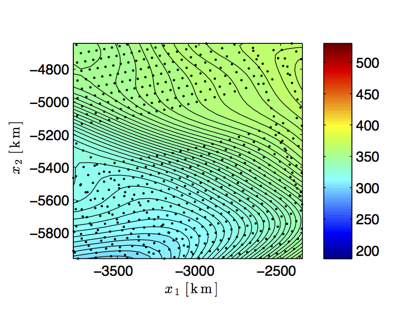
Figure 1: Predicted ozone density $\hat{y}(\mathbf{x})$ in [DU] and training samples (dots) for two different areas. Note both the irregular and gapped sampling pattern.

In the second experiment, we evaluate the inferential properties of the Spice predictor by learning from a small random subset of the data. We use $n=2n^{\prime}=17~{}340$ samples, or approximately $10\%$ of the data. The resulting predictions exhibit discernible patterns as in Fig. 2.

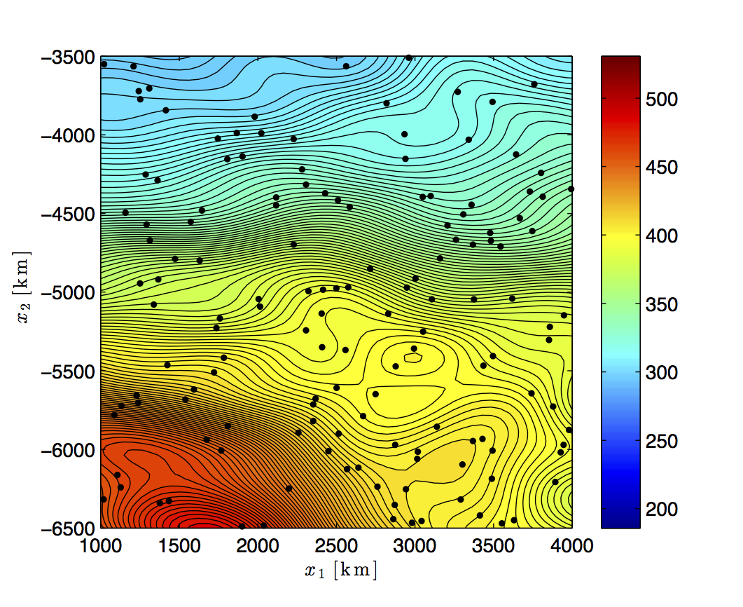
Figure 2: Predicted ozone density $\widehat{y}(\mathbf{x})$ in [DU] and training samples (dots) for two different areas. The predictor was trained using a randomly selected dataset consisting of $5\%$ of the original data.

For a comparison Fig. 3 zooms in on a region with gapped data, also highlighted in Fig. 1. Note that the predictions are consistent with the full data case.

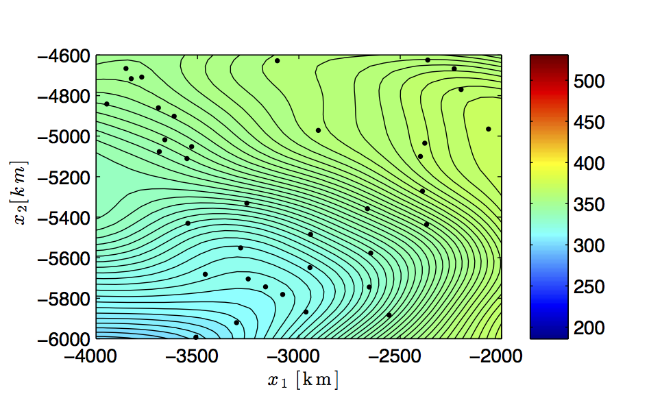
Figure 3: Predicted ozone density $\hat{y}(\mathbf{x})$ in [DU] and training samples (dots). Here $n\approx 0.05n_{0}$ randomly selected training samples are used in contrast with the predictions shown in Fig. 1, which uses the full dataset $n=n_{0}$.

The remaining $\bar{n}=n_{0}-n=164~{}735$ samples are used for validating the predictor. Its risk is estimated by the out-of-sample prediction errors,

$$\widehat{\mathcal{R}}=\widehat{\text{E}}\bigl{[}|y_{i}-\hat{y}(\mathbf{x}_{i})|^{2}\bigr{]},$$

which we translate to Dobson units by taking the square-root. The result was a root-risk of $6.74$ DU. In addition, the confidence interval $C(\mathbf{x})$ with $\kappa=0.90$ had a length of $19.44$ DU and an empirical coverage of 0.90. Both performance metrics compare well with the dynamic range of the data, which spans [179.40, 542.00] or $362$ DU. Fig. 4 also shows that the empirical distribution of the prediction errors is symmetric. These results illustrate the ability of the proposed method to learn, predict and infer in real, large-scale datasets.

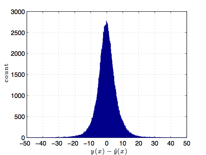
Figure 4: Histogram of the prediction errors for $\bar{n}=164\>735$ samples in [DU]. The predicted samples belong to the interval [179.40, 542.00].

7 Conclusions

In this paper we considered the problem of online learning for prediction problems with large and/or streaming data sets. Starting from a flexible Lc predictor, we formulated a convex covariance-fitting methodology for learning its hyperparameters. The hyperparameters constrain individual weights of the predictor, similar to the automatic relevance determination framework.

It was shown that using the learned hyperparameters results in a predictor with desirable computational and distribution-free properties. We denote it as the Spice predictor. It was implemented online with a runtime that scales linearly in the number of samples, its memory requirement is constant, it avoids local minima issues, and prunes away redundant feature dimensions without relying on assumed properties of the data distributions. In conjunction with the split conformal approach, it also produces distribution-free prediction confidence intervals. Finally, the Spice predictor performance was demonstrated on both real and synthetic datasets, and compared with the offline cross-validation approach.

In future work, we will investigate input-dependent confidence intervals, using the locally-weighted split conformal approach.

Appendix A Derivation of bounds

A.1 Lasso bound (10)

We expand the empirical risk of $\widehat{\mathbf{w}}$ by

$$\begin{split}R&=\widehat{\text{E}}\left[|(y_{i}-\widehat{y}_{\star}(\mathbf{x}_{i}))-(\widehat{y}(\mathbf{x}_{i})-\widehat{y}_{\star}(\mathbf{x}_{i}))|^{2}\right]\\ &=R_{\star}+\Delta_{\star}-2\widehat{\text{E}}[\varepsilon_{i}(\widehat{y}(\mathbf{x}_{i})-\widehat{y}_{\star}(\mathbf{x}_{i}))]\\ &=R_{\star}+\Delta_{\star}-\frac{2}{n}\boldsymbol{\varepsilon}^{\top}\boldsymbol{\Phi}(\widehat{\mathbf{w}}-\mathbf{w}_{\star}).\end{split}$$

Using Hölder’s inequality along with the triangle inequality yields

$$\begin{split}\boldsymbol{\varepsilon}^{\top}\boldsymbol{\Phi}(\widehat{\mathbf{w}}-\mathbf{w}_{\star})&\leq|\boldsymbol{\varepsilon}^{\top}\boldsymbol{\Phi}(\widehat{\mathbf{w}}-\mathbf{w}_{\star})|\leq\|\boldsymbol{\Phi}^{\top}\boldsymbol{\varepsilon}\|_{\infty}\|\widehat{\mathbf{w}}-\mathbf{w}_{\star}\|_{1}\\ &\leq\varepsilon_{\star}(\|\widehat{\mathbf{w}}\|_{1}+\|\mathbf{w}_{\star}\|_{1}).\end{split}$$

Thus, the prediction divergence is bounded by

$$\Delta_{\star}\leq R-R_{\star}+\frac{2\varepsilon_{\star}}{n}(\|\widehat{\mathbf{w}}\|_{1}+\|\mathbf{w}_{\star}\|_{1}).$$ (30)

Next, by inserting $\widehat{\mathbf{w}}$ and $\mathbf{w}_{\star}$ into the cost function of (8), we obtain

$$R-R_{\star}\leq\theta\left(\|\mathbf{w}_{\star}\|_{1}-\|\widehat{\mathbf{w}}\|_{1}\right)$$ (31)

Applying this inequality along with (9) to (30), gives

$$\begin{split}\Delta_{\star}&\leq\theta\left(\|\mathbf{w}_{\star}\|_{1}-\|\widehat{\mathbf{w}}\|_{1}\right)+\theta(\|\widehat{\mathbf{w}}\|_{1}+\|\mathbf{w}_{\star}\|_{1})\\ &=2\theta\|\mathbf{w}_{\star}\|_{1}.\end{split}$$ (32)

Cf. [39] for the case when the unknown data generating mechanism belongs to a sparse linear model class.

A.2 Spice bound (26)

For notational simplicity, we write

$$g(\mathbf{w})=\|\boldsymbol{\varphi}\odot\mathbf{w}\|_{1}=\sum^{p}_{j=1}\varphi_{j}|w_{j}|,$$

since $u=0$. By inserting $\widehat{\mathbf{w}}$ and $\mathbf{w}_{\star}$ into the cost function of (23), we have that

$$\begin{split}R^{1/2}-R^{1/2}_{\star}&\leq\frac{1}{\sqrt{n}}\left(g(\mathbf{w}_{\star})-g(\widehat{\mathbf{w}})\right)\leq\frac{1}{\sqrt{n}}g(\mathbf{w}_{\star}).\end{split}$$ (33)

Multipling the inequality by $R^{1/2}+R^{1/2}_{\star}$ and rearranging, yields

$$\begin{split}R-R_{\star}&\leq\frac{1}{\sqrt{n}}\left(R^{1/2}+R^{1/2}_{\star}\right)(g(\mathbf{w}_{\star})-g(\widehat{\mathbf{w}}))\\ &\leq\frac{1}{\sqrt{n}}\underbrace{\left(2R^{1/2}_{\star}+\frac{1}{\sqrt{n}}g(\mathbf{w}_{\star})\right)}_{\triangleq f(\mathbf{w}_{\star})}(g(\mathbf{w}_{\star})-g(\widehat{\mathbf{w}})),\\ &=\sum_{j}\frac{1}{\sqrt{n}}f(\mathbf{w}_{\star})\varphi_{j}(|w_{\star,j}|-|\widehat{w}_{j}|)\end{split}$$ (34)

where the second inequality follows from using $R^{1/2}\leq R^{1/2}_{\star}+\frac{1}{\sqrt{n}}g(\mathbf{w}_{\star})$ in (33).

Inserting (34) into (30), yields

$$\begin{split}\Delta_{\star}\;&\leq\;\sum_{j}\frac{1}{\sqrt{n}}f(\mathbf{w}_{\star})\varphi_{j}(|w_{\star,j}|-|\widehat{w}_{j}|)+\frac{2\varepsilon_{\star}}{n}(|w_{\star,j}|+|\widehat{w}_{j}|).\end{split}$$ (35)

Given (25), we have that

$$\begin{split}\varphi_{j}&\geq\frac{\varepsilon_{\star}}{\sqrt{nR_{\star}}}\geq\frac{2\varepsilon_{\star}}{\sqrt{n}(2R^{1/2}_{\star}+\frac{1}{\sqrt{n}}g(\mathbf{w}_{\star}))}=\frac{2\varepsilon_{\star}}{\sqrt{n}f(\mathbf{w}_{\star})}\end{split}$$

By re-arranging and dividing by $n$, we obtain the following inequality

$$\begin{split}\frac{1}{\sqrt{n}}f(\mathbf{w}_{\star})\varphi_{j}&\geq\frac{2\varepsilon_{\star}}{n},\quad\forall j>u.\end{split}$$

Therefore (35) can be bounded by

$$\begin{split}\Delta_{\star}\;&\leq\;\sum_{j}\frac{2}{\sqrt{n}}f(\mathbf{w}_{\star})\varphi_{j}|w_{\star,j}|\\ &=\frac{2}{\sqrt{n}}\left(2R^{1/2}_{\star}+\frac{1}{\sqrt{n}}g(\mathbf{w}_{\star})\right)g(\mathbf{w}_{\star})\\ &=4\sqrt{\frac{R_{\star}}{n}}g(\mathbf{w}_{\star})+\frac{2}{n}g^{2}(\mathbf{w}_{\star})\end{split}$$

Note that in the special case when the prediction errors of $\widehat{y}_{\star}(\mathbf{x})$ are i.i.d. $\varepsilon_{i}\sim\mathcal{N}(0,\sigma^{2})$, and the regressors are normalized as $\|\widetilde{\boldsymbol{\phi}}_{j}\|^{2}_{2}\equiv n$, we have that

$$\sqrt{\sigma^{2}(2\ln p+\delta)}\geq\frac{\varepsilon_{\star}}{\sqrt{n}},$$ (36)

with probability greater than $1-2\exp(-\delta/2)$ where $\delta$ is a positive constant, cf. [39, ch. 6.2]. In this setting $R_{\star}$ is a consistent estimate of $\sigma^{2}$. Therefore (25) is satisfied with high probability in this case if the elements of $\boldsymbol{\varphi}$ are multiplied by a factor $c\sqrt{2\ln p+\delta}$, so that

$$\varphi_{j}=\frac{1}{\sqrt{n}}\|\widetilde{\boldsymbol{\phi}}_{j}\|_{2}\times c\sqrt{2\ln p+\delta},$$

for some $c>1$.

Appendix B Optimal weights (16)

The conditional risk can be decomposed as

$$\begin{split}\mathcal{R}(\boldsymbol{\lambda}|\mathbf{x})&=\operatorname{E}[|y-\widehat{y}(\mathbf{x})|^{2}|\mathbf{X},\mathbf{x}]\\ &=\operatorname{Var}[y-\widehat{y}(\mathbf{x})|\mathbf{X},\mathbf{x}]+(\text{Bias}[\widehat{y}(\mathbf{x})])^{2}\\ &=\operatorname{Var}[y|\mathbf{x}]+\operatorname{Var}[\widehat{y}(\mathbf{x})|\mathbf{X}]-2\operatorname{Cov}[y,\widehat{y}(\mathbf{x})|\mathbf{X},\mathbf{x}]]\\ &=K+\operatorname{Var}[\boldsymbol{\lambda}^{\top}\mathbf{y}|\mathbf{X}]-2\operatorname{Cov}[y,\boldsymbol{\lambda}^{\top}\mathbf{y}|\mathbf{X},\mathbf{x}]\\ &=K+\boldsymbol{\lambda}^{\top}\boldsymbol{\Sigma}\boldsymbol{\lambda}-2\boldsymbol{\lambda}^{\top}\mathbf{r}\end{split}$$ (37)

using (15). Here $K$ is a constant and the bias vanishes due to the unbiasedness constraint on $\boldsymbol{\lambda}$. This constraint, in turn, can be expressed as

$$(\mathbf{u}^{\top}(\mathbf{x})-\boldsymbol{\lambda}^{\top}\mathbf{U})\mathbf{w}_{0}=0,\quad\forall\mathbf{w}_{0},$$

or equivalently

$$\mathbf{U}^{\top}\boldsymbol{\lambda}=\mathbf{u}(\mathbf{x}).$$

Note that a weak assumption in our case is $\mathbf{u}(\mathbf{x})\in\mathcal{R}(\mathbf{U}^{\top})$, especially when $n>u$ and $\mathbf{u}(\mathbf{x})\equiv 1$. Hence there exist $\boldsymbol{\lambda}$ that satisfy the equality above.

Thus the problem (12) can be reformulated using the convex Lagrangian

$$\begin{split}L(\boldsymbol{\lambda},\boldsymbol{\kappa})=\boldsymbol{\lambda}^{\top}\boldsymbol{\Sigma}\boldsymbol{\lambda}-2\boldsymbol{\lambda}^{\top}\mathbf{r}+2(\mathbf{U}^{\top}\boldsymbol{\lambda}-\mathbf{u}(\mathbf{x}))^{\top}\boldsymbol{\kappa},\end{split}$$ (38)

where $\boldsymbol{\kappa}$ is the $u\times 1$ vector of Lagrange multipliers.

A stationary point of the Lagrangian in (38) with respect to $\boldsymbol{\lambda}$ and $\boldsymbol{\kappa}$ satisfies

$$\begin{cases}\boldsymbol{\Sigma}\boldsymbol{\lambda}-\mathbf{r}+\mathbf{U}\boldsymbol{\kappa}&=\mathbf{0},\\ \mathbf{U}^{\top}\boldsymbol{\lambda}-\mathbf{u}(\mathbf{x})&=\mathbf{0}.\end{cases}$$

The first equality can be expressed as $\boldsymbol{\lambda}=\boldsymbol{\Sigma}^{-1}(\mathbf{r}-\mathbf{U}\boldsymbol{\kappa})$. We can insert the first equality into the second and solve for the Lagrange multipliers

$$\boldsymbol{\kappa}=-(\mathbf{U}^{\top}\boldsymbol{\Sigma}^{-1}\mathbf{U})^{-}(\mathbf{u}(\mathbf{x})-\mathbf{U}^{\top}\boldsymbol{\Sigma}^{-1}\mathbf{r}).$$

Then we have

$$\begin{split}\boldsymbol{\lambda}&=\boldsymbol{\Sigma}^{-1}\mathbf{r}+\boldsymbol{\Sigma}^{-1}\mathbf{U}(\mathbf{U}^{\top}\boldsymbol{\Sigma}^{-1}\mathbf{U})^{-}\mathbf{u}(\mathbf{x})\\ &\quad-\boldsymbol{\Sigma}^{-1}\mathbf{U}(\mathbf{U}^{\top}\boldsymbol{\Sigma}^{-1}\mathbf{U})^{-}\mathbf{U}^{\top}\boldsymbol{\Sigma}^{-1}\mathbf{r}.\end{split}$$

Noting that the orthogonal projector is given by $\boldsymbol{\Pi}^{\perp}=\mathbf{I}-\mathbf{U}(\mathbf{U}^{\top}\boldsymbol{\Sigma}^{-1}\mathbf{U})^{-}\mathbf{U}^{\top}\boldsymbol{\Sigma}^{-1}$ concludes the proof.

Appendix C Linear regression form (19)

Let $\boldsymbol{\phi}(\mathbf{x})$ be partitioned as in (18). Then

$$\widehat{y}(\mathbf{x})=\boldsymbol{\lambda}^{\top}(\mathbf{x})\mathbf{y}=\boldsymbol{\phi}^{\top}(\mathbf{x})\widehat{\mathbf{w}}$$

in combination with (16) allows us to identify the weights:

$$\widehat{\mathbf{w}}=\begin{bmatrix}\widehat{\mathbf{w}}_{0}\\ \widehat{\mathbf{w}}_{1}\end{bmatrix}=\begin{bmatrix}(\mathbf{U}^{\top}\boldsymbol{\Sigma}^{-1}\mathbf{U})^{\dagger}\mathbf{U}^{\top}\boldsymbol{\Sigma}^{-1}\mathbf{y}\\ \boldsymbol{\Theta}\boldsymbol{\Psi}^{\top}\boldsymbol{\Sigma}^{-1}(\mathbf{y}-\mathbf{U}\widehat{\mathbf{w}}_{0})\end{bmatrix}.$$ (39)

Next, define the problem

$$\min_{\mathbf{w}_{0},\>\mathbf{w}_{1},}\;\theta^{-1}_{0}\|\mathbf{y}-\mathbf{U}\mathbf{w}_{0}-\boldsymbol{\Psi}\mathbf{w}_{1}\|^{2}_{2}+\|\mathbf{w}_{1}\|^{2}_{\boldsymbol{\Theta}^{-1}}$$ (40)

for which the minimizing $\mathbf{w}_{1}$, namely,

$$\begin{split}\widehat{\mathbf{w}}_{1}&=\theta^{-1}_{0}(\theta^{-1}_{0}\boldsymbol{\Psi}\boldsymbol{\Psi}^{\top}+\boldsymbol{\Theta}^{-1})^{-1}\boldsymbol{\Psi}^{\top}(\mathbf{y}-\mathbf{U}\mathbf{w}_{0})\\ &=\theta^{-1}_{0}(\boldsymbol{\Theta}-\boldsymbol{\Theta}\boldsymbol{\Psi}^{\top}\boldsymbol{\Sigma}^{-1}\boldsymbol{\Psi}\boldsymbol{\Theta})\boldsymbol{\Psi}^{\top}(\mathbf{y}-\mathbf{U}\mathbf{w}_{0})\\ &=\theta^{-1}_{0}\boldsymbol{\Theta}\boldsymbol{\Psi}^{\top}\boldsymbol{\Sigma}^{-1}(\boldsymbol{\Sigma}-\boldsymbol{\Psi}\boldsymbol{\Theta}\boldsymbol{\Psi}^{\top})(\mathbf{y}-\mathbf{U}\mathbf{w}_{0})\\ &=\boldsymbol{\Theta}\boldsymbol{\Psi}^{\top}\boldsymbol{\Sigma}^{-1}(\mathbf{y}-\mathbf{U}\mathbf{w}_{0}),\end{split}$$

has the same form as in (39) with $\mathbf{w}_{0}$ still to be determined. In the above calculation we made use of the matrix inversion lemma. Inserting $\widehat{\mathbf{w}}_{1}$ back into (40) yields the concentrated cost function

$$\begin{split}&\theta^{-1}_{0}\|\mathbf{y}-\mathbf{U}\mathbf{w}_{0}-\boldsymbol{\Psi}\widehat{\mathbf{w}}_{1}\|^{2}_{2}+\|\widehat{\mathbf{w}}_{1}\|^{2}_{\boldsymbol{\Theta}^{-1}}\\ =&\theta^{-1}_{0}\|(\mathbf{I}_{N}-\boldsymbol{\Psi}\boldsymbol{\Theta}\boldsymbol{\Psi}^{\top}\boldsymbol{\Sigma}^{-1})(\mathbf{y}-\mathbf{U}\mathbf{w}_{0})\|^{2}_{2}\\ &\quad+\|\boldsymbol{\Theta}\boldsymbol{\Psi}^{\top}\boldsymbol{\Sigma}^{-1}(\mathbf{y}-\mathbf{U}\mathbf{w}_{0})\|^{2}_{\boldsymbol{\Theta}^{-1}}\\ =&\theta_{0}(\mathbf{y}-\mathbf{U}\mathbf{w}_{0})^{\top}\boldsymbol{\Sigma}^{-1}\boldsymbol{\Sigma}^{-1}(\mathbf{y}-\mathbf{U}\mathbf{w}_{0})\\ &\quad+(\mathbf{y}-\mathbf{U}\mathbf{w}_{0})^{\top}\boldsymbol{\Sigma}^{-1}\boldsymbol{\Psi}\boldsymbol{\Theta}\boldsymbol{\Psi}^{\top}\boldsymbol{\Sigma}^{-1}(\mathbf{y}-\mathbf{U}\mathbf{w}_{0})\\ =&(\mathbf{y}-\mathbf{U}\mathbf{w}_{0})^{\top}\boldsymbol{\Sigma}^{-1}(\mathbf{y}-\mathbf{U}\mathbf{w}_{0}).\end{split}$$

Minimizing with respect to $\mathbf{w}_{0}$ yields $\widehat{\mathbf{w}}_{0}$ in (39). Finally, multiplying the cost function (40) by $\theta_{0}/n$ yield the desired form.

Appendix D Convexity of learning problem (20)

By expanding the criterion (20) we obtain

$$\widetilde{\mathbf{y}}^{\top}\boldsymbol{\Sigma}^{-1}\widetilde{\mathbf{y}}+\operatorname{tr}\{\boldsymbol{\Sigma}\}$$ (41)

where $\widetilde{\mathbf{y}}=\mathbf{y}-\mathbf{U}\mathbf{w}_{0}$.

We note that $\boldsymbol{\Sigma}$ in (15) is a linear function of $\boldsymbol{\theta}$. Thus the normalization constraint (21) can be written as a linear equality constraint

$$n\theta_{0}+\sum^{q}_{j=1}\|\widetilde{\boldsymbol{\phi}}_{j}\|^{2}\theta_{j}=\rho$$ (42)

Next, we define an auxiliary variable $\alpha$ that satisfies

$$\alpha\geq\widetilde{\mathbf{y}}^{\top}\boldsymbol{\Sigma}^{-1}\widetilde{\mathbf{y}},$$

or equivalently

$$\begin{bmatrix}\alpha&\widetilde{\mathbf{y}}^{\top}\\ \widetilde{\mathbf{y}}&\boldsymbol{\Sigma}\end{bmatrix}\succeq\mathbf{0}.$$ (43)

Using the auxiliary variable and the definition of $\boldsymbol{\Sigma}$, we can therefore reformulate the learning problem

$$\min_{\alpha,\>\boldsymbol{\theta}}\;\alpha+n\theta_{0}+\sum^{q}_{j=1}\|\widetilde{\boldsymbol{\phi}}_{j}\|^{2}\theta_{j},$$

which has a linear cost function and is subject to the constraints (42) and (43). This problem is recognized as a semidefinite program, i.e. it is convex. See [58] and [27].

Appendix E Spice predictor (22)

The derivation follows in three steps. First we show that dropping the constraint (21) yields the simpler unconstrained problem in (20). Next, we prove that the fitted hyperparameters in the simplified problem yields the same predictor. Finally, we show how the corresponding Lr form arises as a consequence.

By dropping the constraint (21) we may consider the problem in the following form:

$$\widehat{\boldsymbol{\theta}}=\operatorname*{arg\,min}_{\boldsymbol{\theta}}\>\operatorname{tr}\{\mathbf{Z}\boldsymbol{\Sigma}^{-1}\}+\operatorname{tr}\{\boldsymbol{\Sigma}\},$$ (44)

where $\mathbf{Z}$ is the unnormalized sample covariance matrix.

We now prove that, $\boldsymbol{\theta}^{\star}\propto\widehat{\boldsymbol{\theta}}$. Begin by defining a constant $\kappa>0$, such that $\text{tr}\{\mathbf{Z}\boldsymbol{\Sigma}^{-1}(\widehat{\boldsymbol{\theta}})\}=\kappa^{2}\text{tr}\{\boldsymbol{\Sigma}(\widehat{\boldsymbol{\theta}})\}$ at the minimum of (44). We show that $\kappa=1$ is the only possible value and so both terms in (44) equal each other at the minimum.

Let $\tilde{\boldsymbol{\theta}}=\kappa\widehat{\boldsymbol{\theta}}$, and observe that the cost (44) is then bounded by

$$\begin{split}(\kappa^{2}+1)\text{tr}\{\boldsymbol{\Sigma}(\widehat{\boldsymbol{\theta}})\}&\leq\text{tr}\{\mathbf{Z}\boldsymbol{\Sigma}^{-1}(\tilde{\boldsymbol{\theta}})\}+\text{tr}\{\boldsymbol{\Sigma}(\tilde{\boldsymbol{\theta}})\}\\ &=\kappa^{-1}\text{tr}\{\mathbf{Z}\boldsymbol{\Sigma}^{-1}(\widehat{\boldsymbol{\theta}})\}+\kappa\text{tr}\{\boldsymbol{\Sigma}(\widehat{\boldsymbol{\theta}})\}\\ &=2\kappa\text{tr}\{\boldsymbol{\Sigma}(\widehat{\boldsymbol{\theta}})\}.\end{split}$$

Thus $\kappa$ must satisfy $\kappa^{2}+1\leq 2\kappa$, or $(\kappa-1)^{2}\leq 0$. Therefore $\kappa=1$ is the only solution and both terms must be equal at the minimum. We can thus re-write the minimization of (44) as the following problem

$$\begin{split}\min&\quad\alpha\\ \text{subject to}&\quad\text{tr}\{\mathbf{Z}\boldsymbol{\Sigma}^{-1}\}=\alpha,\;\text{tr}\{\boldsymbol{\Sigma}\}=\alpha,\end{split}$$ (45)

with minimizer $\hat{\boldsymbol{\theta}}$ and where $\alpha>0$ is an auxiliary variable.

Next, consider an equivalent problem to (45) obtained by re-defining the variables as $\tilde{\boldsymbol{\theta}}=\rho\alpha^{-1}\boldsymbol{\theta}$. Then $\text{tr}\{\mathbf{Z}\boldsymbol{\Sigma}^{-1}(\boldsymbol{\theta})\}=\rho\alpha^{-1}\text{tr}\{\mathbf{Z}\boldsymbol{\Sigma}^{-1}(\tilde{\boldsymbol{\theta}})\}$ and $\text{tr}\{\boldsymbol{\Sigma}(\boldsymbol{\theta})\}=\alpha\rho^{-1}\text{tr}\{\boldsymbol{\Sigma}(\tilde{\boldsymbol{\theta}})\}$, so that the equivalent problem becomes

$$\begin{split}\min&\quad\beta\\ \text{subject to}&\quad\text{tr}\{\mathbf{Z}\boldsymbol{\Sigma}^{-1}\}=\beta,\;\text{tr}\{\boldsymbol{\Sigma}\}=\rho,\end{split}$$ (46)

where $\beta=\alpha^{2}\rho^{-1}$. The minimizer of the equivalent problem (46) is therefore $\tilde{\boldsymbol{\theta}}\propto\widehat{\boldsymbol{\theta}}$. Problem (46) is however identical to the constrained problem

$$\begin{split}\min&\quad\text{tr}\{\mathbf{Z}\boldsymbol{\Sigma}^{-1}\}\\ \text{subject to}&\quad\text{tr}\{\boldsymbol{\Sigma}\}=\rho,\end{split}$$

whose minimizer is $\tilde{\boldsymbol{\theta}}=\boldsymbol{\theta}^{\star}$, which follows from expanding the cost in (20) and the constraint (21).

Thus we proved that $\boldsymbol{\theta}^{\star}\propto\widehat{\boldsymbol{\theta}}$. Next, note that the optimal Lc predictor based on (16) is invariant to uniform scaling of $\boldsymbol{\theta}$. That is, $\widehat{y}(\mathbf{x};\boldsymbol{\theta})=\widehat{y}(\mathbf{x};c\boldsymbol{\theta})$ for all $c>0$. The result follows readily by inspection of the minimizer (19), given in (39). Therefore

$$\widehat{y}(\mathbf{x};\boldsymbol{\theta}^{\star})=\widehat{y}(\mathbf{x};\widehat{\boldsymbol{\theta}}).$$

Finally, consider the following augmented problem

$$\min_{\mathbf{w}_{0},\>\mathbf{w}_{1},\>\boldsymbol{\theta}}\;\theta^{-1}_{0}\|\mathbf{y}-\mathbf{U}\mathbf{w}_{0}-\boldsymbol{\Psi}\mathbf{w}_{1}\|^{2}_{2}+\|\mathbf{w}_{1}\|^{2}_{\boldsymbol{\Theta}^{-1}}+\text{tr}\{\boldsymbol{\Sigma}\}.$$ (47)

Solving for $\mathbf{w}_{0}$ and $\mathbf{w}_{1}$ yields the minimizer (19), i.e., (39). Moreover, by inserting the minimizing $\mathbf{w}_{1}$ back into (47) we obtain the concentrated cost function

$$\begin{split}&\theta^{-1}_{0}\|(\mathbf{I}_{n}-\boldsymbol{\Psi}\boldsymbol{\Theta}\boldsymbol{\Psi}^{\top}\boldsymbol{\Sigma}^{-1})(\mathbf{y}-\mathbf{U}\mathbf{w}_{0})\|^{2}_{2}\\ &\quad+\|\boldsymbol{\Theta}\boldsymbol{\Psi}^{\top}\boldsymbol{\Sigma}^{-1}(\mathbf{y}-\mathbf{U}\mathbf{w}_{0})\|^{2}_{\boldsymbol{\Theta}^{-1}}+\text{tr}\{\boldsymbol{\Sigma}\}\\ =&\theta_{0}(\mathbf{y}-\mathbf{U}\mathbf{w}_{0})^{\top}\boldsymbol{\Sigma}^{-1}\boldsymbol{\Sigma}^{-1}(\mathbf{y}-\mathbf{U}\mathbf{w}_{0})\\ &\quad+(\mathbf{y}-\mathbf{U}\mathbf{w}_{0})^{\top}\boldsymbol{\Sigma}^{-1}\boldsymbol{\Psi}\boldsymbol{\Theta}\boldsymbol{\Psi}^{\top}\boldsymbol{\Sigma}^{-1}(\mathbf{y}-\mathbf{U}\mathbf{w}_{0})+\text{tr}\{\boldsymbol{\Sigma}\}\\ =&\text{tr}\{(\mathbf{y}-\mathbf{U}\mathbf{w}_{0})(\mathbf{y}-\mathbf{U}\mathbf{w}_{0})^{\top}\boldsymbol{\Sigma}^{-1}\}+\text{tr}\{\boldsymbol{\Sigma}\}\end{split}$$

which is equal to that in (44). Thus the augmented problem (47) enables us to obtain both $\widehat{\boldsymbol{\theta}}$ and $\widehat{\mathbf{w}}$.

Using the result above, we may alternatively solve for $\boldsymbol{\theta}$ first. The second and third terms in (44) can be written as

$$\|\mathbf{w}_{1}\|^{2}_{\boldsymbol{\Theta}^{-1}}=\sum^{q}_{k=1}\frac{1}{\theta_{k}}w^{2}_{u+k}$$

and

$$\begin{split}\text{tr}\{\boldsymbol{\Sigma}\}&=\text{tr}\{\boldsymbol{\Psi}^{\top}\boldsymbol{\Psi}\boldsymbol{\Theta}\}+\operatorname{tr}\{\theta_{0}\mathbf{I}_{n}\}\\ &=\sum^{q}_{k=1}\|\widetilde{\boldsymbol{\phi}}_{u+k}\|^{2}_{2}\theta_{k}+n\theta_{0},\end{split}$$

respectively. Then the minimizing hyperparameters $\boldsymbol{\theta}$ in (47) can be expressed in closed-form:

$$\hat{\theta}_{k}=\begin{cases}\|\mathbf{y}-\boldsymbol{\Phi}\mathbf{z}\|_{2}/\sqrt{n},\quad k=0.\\ |w_{u+k}|/\|\widetilde{\boldsymbol{\phi}}_{u+k}\|_{2},\quad k=1,\dots,q.\end{cases}$$

Inserting the expression back in to (47) yields a concentrated cost function

$$\sqrt{\|\mathbf{y}-\boldsymbol{\Phi}\mathbf{w}\|^{2}_{2}}+\sum^{p}_{j=u+1}\frac{1}{\sqrt{n}}\|\widetilde{\boldsymbol{\phi}}_{j}\|_{2}|w_{j}|$$

which, after dividing by $n^{-1/2}$, equals that in (23). Thus the right hand side of (22) yields $\widehat{y}(\mathbf{x};\widehat{\boldsymbol{\theta}})$ when using $\widehat{\boldsymbol{\theta}}$ from (44).

Appendix F Online algorithm

Proof.

We reformulate the convex problem in (23) at a given sample size $n$, using (27). We solve the problem in (23) via cyclic minimization [28]. That is, we minimize the cost function, with respect to one variable $w_{j}$ at a time, while holding the remaining variables $\{w_{k}\}_{k\neq j}$ are held constant [52].

Recall that $\widetilde{\boldsymbol{\phi}}_{j}$ is the $j$th column of $\boldsymbol{\Phi}$ and

$$\overline{\mathbf{y}}_{j}=\mathbf{y}-\sum_{k\neq j}\widetilde{\boldsymbol{\phi}}_{k}\check{w}_{k},$$

where $\check{w}_{k}$ is the current estimate of $w_{k}$. (When $n=0$, the initial estimate $\check{w}_{j}$ is set to 0.) Starting from the cost in (23), we define an equivalent cost function with respect to $w_{j}$:

$$V(w_{j})\triangleq\|\overline{\mathbf{y}}_{j}-\widetilde{\boldsymbol{\phi}}_{j}w_{j}\|_{2}+\varphi_{j}|w_{j}|,$$ (48)

where

$$\varphi_{j}=\begin{cases}0,\quad\quad j\leq u\\ \|\widetilde{\boldsymbol{\phi}}_{j}\|_{2}/\sqrt{n},\quad j>u\\ \end{cases}.$$

Now consider two cases:

Case 1) when $j=1,\dots,u$: Then $\varphi_{j}=0$ and (48) can be written as

$$V(w_{j})=(\|\overline{\mathbf{y}}_{j}\|^{2}+\|\widetilde{\boldsymbol{\phi}}_{j}\|^{2}w^{2}_{j}-2\widetilde{\boldsymbol{\phi}}^{\top}_{j}\overline{\mathbf{y}}_{j}w_{j})^{1/2}.$$ (49)

The minimizer of (49) is readily found as $\hat{w}_{j}=\widetilde{\boldsymbol{\phi}}^{\top}_{j}\overline{\mathbf{y}}_{j}/\|\widetilde{\boldsymbol{\phi}}_{j}\|^{2}$ and we get a nonnegative expression $(\|\widetilde{\boldsymbol{\phi}}_{j}\|^{2}\|\overline{\mathbf{y}}_{j}\|^{2}-(\widetilde{\boldsymbol{\phi}}^{\top}_{j}\overline{\mathbf{y}}_{j})^{2})/\|\widetilde{\boldsymbol{\phi}}_{j}\|^{2}\geq 0$ inside the brackets of $V(\hat{w}_{j})$ using the Cauchy-Schwartz inequality. Noting that $\overline{\mathbf{y}}_{j}=\mathbf{y}-\boldsymbol{\Phi}\check{\mathbf{w}}+\widetilde{\boldsymbol{\phi}}_{j}\check{w}_{j}$, we can express the minimizer as

$$\begin{split}\hat{w}_{j}&=\frac{\widetilde{\boldsymbol{\phi}}^{\top}_{j}(\mathbf{y}-\boldsymbol{\Phi}\check{\mathbf{w}}+\widetilde{\boldsymbol{\phi}}_{j}\check{w}_{j})}{\|\widetilde{\boldsymbol{\phi}}_{j}\|^{2}}=\frac{\zeta_{j}+\Gamma_{jj}\check{w}_{j}}{\Gamma_{jj}},\end{split}$$ (50)

where we have defined the vector

$$\boldsymbol{\zeta}\triangleq\boldsymbol{\rho}-\boldsymbol{\Gamma}\check{\boldsymbol{\mathbf{z}}}.$$

Case 2) when $j=u+1,\dots,p$: We parameterize the variable $w_{j}$ as $w_{j}=s_{i}r_{j}$, where $r_{j}\geq 0$ and $s_{j}\in\{-1,1\}$. Then (48) becomes

$$\begin{split}V(r_{j},s_{j})&=(\|\bar{\mathbf{y}}_{j}\|^{2}+\|\widetilde{\boldsymbol{\phi}}_{j}\|^{2}r^{2}_{j}-2\widetilde{\boldsymbol{\phi}}^{\top}_{j}\overline{\mathbf{y}}_{j}s_{j}r_{j})^{1/2}+\varphi_{j}r_{j},\end{split}$$

The minimizing $s_{j}$ is given by

$$\begin{split}\hat{s}_{j}&=\text{sign}(\widetilde{\boldsymbol{\phi}}^{\top}_{j}\overline{\mathbf{y}}_{j})\\ &=\text{sign}(\widetilde{\boldsymbol{\phi}}^{\top}_{j}(\mathbf{y}-\boldsymbol{\Phi}\check{\mathbf{w}}+\widetilde{\boldsymbol{\phi}}_{j}\check{w}_{j}))\\ &=\text{sign}(\zeta_{j}+\Gamma_{jj}\check{w}_{j}).\end{split}$$ (51)

To write the minimizing $r_{i}$ in a compact manner, we introduce the following variables

$$\begin{split}\xi&\triangleq\|\mathbf{y}-\boldsymbol{\Phi}\check{\mathbf{w}}\|^{2}\\ &=\kappa+\check{\mathbf{w}}^{\top}\boldsymbol{\Gamma}\check{\mathbf{w}}-2\check{\mathbf{w}}^{\top}\boldsymbol{\rho}\end{split}$$

and

$$\begin{split}\alpha_{j}&\triangleq\|\overline{\mathbf{y}}_{j}\|^{2}\\ &=\|\mathbf{y}-\boldsymbol{\Phi}\check{\mathbf{w}}+\widetilde{\boldsymbol{\phi}}_{j}\check{w}_{j}\|^{2}\\ &=\xi+\Gamma_{jj}\check{z}^{2}_{j}+2\check{w}_{j}\zeta_{j},\\ \beta_{j}&\triangleq\|\widetilde{\boldsymbol{\phi}}_{j}\|^{2}\\ &=\Gamma_{jj},\\ \gamma_{j}&\triangleq|\widetilde{\boldsymbol{\phi}}^{\top}_{j}\overline{\mathbf{y}}_{j}|\\ &=|\widetilde{\boldsymbol{\phi}}^{\top}_{j}(\mathbf{y}-\boldsymbol{\Phi}\check{\mathbf{w}}+\widetilde{\boldsymbol{\phi}}_{j}\check{w}_{j})|\\ &=|\zeta_{j}+\Gamma_{jj}\check{w}_{j}|.\\ \end{split}$$ (52)

The use of this notation enables us to express the concentrated cost function as

$$\begin{split}V(r_{j},\hat{s}_{j})&=(\alpha_{j}+\beta_{j}r^{2}_{j}-2\gamma_{j}r_{j})^{1/2}+\varphi_{j}r_{j}.\end{split}$$ (53)

It was shown in [28, sec. III] that the minimizer of (53) is

$$\begin{split}\hat{r}_{j}&=\frac{\gamma_{j}}{\beta_{j}}-\frac{1}{\beta_{j}}\left(\frac{\alpha_{j}\beta_{j}-\gamma^{2}_{j}}{n-1}\right)^{1/2},\end{split}$$ (54)

when $\sqrt{n-1}\gamma_{j}>\sqrt{\alpha_{j}\beta_{j}-\gamma^{2}_{j}}$. Otherwise $\hat{r}_{j}=0$. More compactly,

$$\hat{w}_{j}=\begin{cases}\hat{s}_{j}\hat{r}_{j},&\text{if }\sqrt{n-1}\gamma_{j}>\sqrt{\alpha_{j}\beta_{j}-\gamma^{2}_{j}}\\ 0,&\text{else},\end{cases}$$ (55)

using (51), (52) and (54).

In summary, at sample $n$ the cyclic minimizer for problem (23) consists of the iterative application of (50) and (55). As each element $\hat{w}_{i}$ is updated, the convex cost function in (23) decreases monotonically by a general property of cyclic minimizers. Therefore by repeating the updates $L$ times, the solution will converge to $\widehat{\mathbf{w}}$ in (23) as $L$ increases. Note that all the variables in (50) and (55), are based on the variables (27).

∎

References

• [1] T. Hastie, R. Tibshirani, and J. Friedman, The Elements of Statistical Learning: Data Mining, Inference, and Prediction, Second Edition. Springer Series in Statistics, Springer New York, 2009.
• [2] N. Cressie and C. Wikle, Statistics for Spatio-Temporal Data. CourseSmart Series, Wiley, 2011.
• [3] T. Söderström and P. Stoica, System Identification. Prentice-Hall, Inc., 1988.
• [4] K. Murphy, Machine Learning: A Probabilistic Perspective. Adaptive computation and machine learning series, MIT Press, 2012.
• [5] H. Wold, A Study in the Analysis of Stationary Time Series. Almqvist and Wiksells, 1938.
• [6] A. Kolmogorov, “Interpolation and extrapolation of stationary random sequences,” Izvestiia Akademii Nauk SSR, Seriia Matematicheskaia, vol. 5, pp. 3–14, 1941.
• [7] N. Wiener, Extrapolation, Interpolation and Smoothing of Stationary Time Series. MIT Press, 1949.
• [8] N. Cressie, “The origins of kriging,” Mathematical Geology, vol. 22, no. 3, pp. 239–252, 1990.
• [9] A. E. Hoerl and R. W. Kennard, “Ridge regression: Biased estimation for nonorthogonal problems,” Technometrics, vol. 12, no. 1, pp. 55–67, 1970.
• [10] R. Tibshirani, “Regression shrinkage and selection via the lasso,” Journal of the Royal Statistical Society. Series B (Methodological), pp. 267–288, 1996.
• [11] H. Zou and T. Hastie, “Regularization and variable selection via the elastic net,” Journal of the Royal Statistical Society: Series B (Statistical Methodology), vol. 67, no. 2, pp. 301–320, 2005.
• [12] E. A. Nadaraya, “On estimating regression,” Theory of Probability & Its Applications, vol. 9, no. 1, pp. 141–142, 1964.
• [13] G. S. Watson, “Smooth regression analysis,” Sankhyā: The Indian Journal of Statistics, Series A, pp. 359–372, 1964.
• [14] H. Drucker, C. J. Burges, L. Kaufman, A. Smola, and V. Vapnik, “Support vector regression machines,” Advances in Neural Information Processing Systems (NIPS), vol. 9, pp. 155–161, 1997.
• [15] C. K. Williams and C. E. Rasmussen, “Gaussian processes for regression,” Advances in Neural Information Processing Systems, vol. 8, pp. 514–520, 1996.
• [16] W. S. Cleveland, “LOWESS: A program for smoothing scatterplots by robust locally weighted regression,” The American Statistician, vol. 35, no. 1, p. 54, 1981.
• [17] D. J. MacKay, Information theory, inference and learning algorithms. Cambridge university press, 2003.
• [18] N. Cressie, “Fitting variogram models by weighted least squares,” Journal of the International Association for Mathematical Geology, vol. 17, no. 5, pp. 563–586, 1985.
• [19] B. Efron and R. Tibshirani, “Bootstrap methods for standard errors, confidence intervals, and other measures of statistical accuracy,” Statistical science, pp. 54–75, 1986.
• [20] V. Vovk, A. Gammerman, and G. Shafer, Algorithmic learning in a random world. Springer Science & Business Media, 2005.
• [21] J. Lei, M. G’Sell, A. Rinaldo, R. J. Tibshirani, and L. Wasserman, “Distribution-free predictive inference for regression,” arXiv preprint arXiv:1604.04173, 2016.
• [22] R. M. Neal, Bayesian learning for neural networks, vol. 118. Springer Science & Business Media, 1996.
• [23] M. E. Tipping, “Sparse Bayesian learning and the relevance vector machine,” Journal of machine learning research, vol. 1, no. Jun, pp. 211–244, 2001.
• [24] T. W. Anderson, “Linear latent variable models and covariance structures,” Journal of Econometrics, vol. 41, no. 1, pp. 91–119, 1989.
• [25] B. Ottersten, P. Stoica, and R. Roy, “Covariance matching estimation techniques for array signal processing applications,” Digital Signal Processing, vol. 8, no. 3, pp. 185–210, 1998.
• [26] P. Stoica, P. Babu, and J. Li, “New method of sparse parameter estimation in separable models and its use for spectral analysis of irregularly sampled data,” IEEE Trans. Signal Processing, vol. 59, no. 1, pp. 35–47, 2011.
• [27] P. Stoica, P. Babu, and J. Li, “SPICE: A sparse covariance-based estimation method for array processing,” IEEE Trans. Signal Processing, vol. 59, no. 2, pp. 629–638, 2011.
• [28] D. Zachariah and P. Stoica, “Online hyperparameter-free sparse estimation method,” IEEE Trans. Signal Processing, vol. 63, pp. 3348–3359, July 2015.
• [29] L. Wasserman, All of Statistics: A Concise Course in Statistical Inference. Springer Texts in Statistics, Springer New York, 2004.
• [30] M. Stein, Interpolation of Spatial Data: Some Theory for Kriging. Springer Series in Statistics, Springer New York, 1999.
• [31] K. Mardia and A. Watkins, “On multimodality of the likelihood in the spatial linear model,” Biometrika, vol. 76, no. 2, pp. 289–295, 1989.
• [32] R. Zimmermann, “Asymptotic behavior of the likelihood function of covariance matrices of spatial Gaussian processes,” Journal of Applied Mathematics, vol. 2010, 2011.
• [33] C. Rasmussen and C. Williams, Gaussian Processes for Machine Learning. Adaptative computation and machine learning series, MIT Press, 2006.
• [34] R. J. Carroll and D. Ruppert, “A comparison between maximum likelihood and generalized least squares in a heteroscedastic linear model,” Journal of the American Statistical Association, vol. 77, no. 380, pp. 878–882, 1982.
• [35] D. Lazer, R. Kennedy, G. King, and A. Vespignani, “The parable of Google flu: traps in big data analysis,” Science, vol. 343, no. 6176, pp. 1203–1205, 2014.
• [36] J. Weston, A. Elisseeff, B. Schölkopf, and M. Tipping, “Use of the zero-norm with linear models and kernel methods,” Journal of machine learning research, vol. 3, no. Mar, pp. 1439–1461, 2003.
• [37] D. P. Foster and E. I. George, “The risk inflation criterion for multiple regression,” The Annals of Statistics, pp. 1947–1975, 1994.
• [38] T. Hastie, R. Tibshirani, and M. Wainwright, Statistical learning with sparsity. CRC press, 2015.
• [39] P. Bühlmann and S. Van De Geer, Statistics for high-dimensional data: methods, theory and applications. Springer Science & Business Media, 2011.
• [40] E. Greenshtein and Y. Ritov, “Persistence in high-dimensional linear predictor selection and the virtue of overparametrization,” Bernoulli, vol. 10, no. 6, pp. 971–988, 2004.
• [41] D. Angelosante, J. A. Bazerque, and G. B. Giannakis, “Online adaptive estimation of sparse signals: Where RLS meets the $\ell_{1}$-norm,” IEEE Transactions on Signal Processing, vol. 58, no. 7, pp. 3436–3447, 2010.
• [42] A. Rahimi and B. Recht, “Random features for large-scale kernel machines,” in Advances in neural information processing systems, pp. 1177–1184, 2007.
• [43] A. Solin and S. Särkkä, “Hilbert space methods for reduced-rank Gaussian process regression,” 2014. arXiv preprint arXiv:1401.5508.
• [44] A. Shah, A. G. Wilson, and Z. Ghahramani, “Student-t processes as alternatives to gaussian processes.,” in AISTATS, pp. 877–885, 2014.
• [45] X. Y. Felix, A. T. Suresh, K. M. Choromanski, D. N. Holtmann-Rice, and S. Kumar, “Orthogonal random features,” in Advances in Neural Information Processing Systems (NIPS), pp. 1975–1983, 2016.
• [46] A. C. Faul and M. E. Tipping, “Analysis of sparse bayesian learning,” Advances in Neural Information Processing Systems (NIPS), vol. 1, pp. 383–390, 2002.
• [47] D. P. Wipf and S. S. Nagarajan, “A new view of automatic relevance determination,” in Advances in Neural Information Processing Systems 20 (J. C. Platt, D. Koller, Y. Singer, and S. T. Roweis, eds.), pp. 1625–1632, Curran Associates, Inc., 2008.
• [48] P. Stoica, D. Zachariah, and J. Li, “Weighted SPICE: A unifying approach for hyperparameter-free sparse estimation,” Digital Signal Processing, vol. 33, pp. 1–12, 2014.
• [49] A. Belloni, V. Chernozhukov, and L. Wang, “Square-root lasso: pivotal recovery of sparse signals via conic programming,” Biometrika, vol. 98, no. 4, pp. 791–806, 2011.
• [50] M. Hong, M. Razaviyayn, Z.-Q. Luo, and J.-S. Pang, “A unified algorithmic framework for block-structured optimization involving big data: With applications in machine learning and signal processing,” IEEE Signal Processing Magazine, vol. 33, no. 1, pp. 57–77, 2016.
• [51] W. I. Zangwill, Nonlinear Programming: a Unified Approach. Prentice-Hall Englewood Cliffs, NJ, 1969.
• [52] P. Stoica and Y. Selén, “Cyclic minimizers, majorization techniques, and the expectation-maximization algorithm: a refresher,” IEEE Signal Processing Magazine, vol. 21, no. 1, pp. 112–114, 2004.
• [53] D. P. Wipf and B. D. Rao, “An empirical bayesian strategy for solving the simultaneous sparse approximation problem,” IEEE Transactions on Signal Processing, vol. 55, no. 7, pp. 3704–3716, 2007.
• [54] J. Wågberg, D. Zachariah, T. B. Schön, and P. Stoica, “Prediction performance after learning in Gaussian process regression,” in AISTATS, p. xxx, 2014.
• [55] R. D. McPeters, P. Bhartia, A. J. Krueger, J. R. Herman, B. M. Schlesinger, C. G. Wellemeyer, C. J. Seftor, G. Jaross, S. L. Taylor, T. Swissler, et al., Nimbus-7 Total Ozone Mapping Spectrometer (TOMS) data products user’s guide, vol. 1384. National Aeronautics and Space Administration, Scientific and Technical Information Branch, 1996.
• [56] N. Cressie and G. Johannesson, “Fixed rank kriging for very large spatial data sets,” Journal of the Royal Statistical Society: Series B (Statistical Methodology), vol. 70, no. 1, pp. 209–226, 2008.
• [57] J. P. Snyder, Map projections–A working manual, vol. 1395. US Government Printing Office, 1987.
• [58] M. S. Lobo, L. Vandenberghe, S. Boyd, and H. Lebret, “Applications of second-order cone programming,” Linear algebra and its applications, vol. 284, no. 1-3, pp. 193–228, 1998.