Single-photon double ionization: renormalized-natural-orbital theory vs multi-configurational Hartree-Fock

Abstract

The $N$-particle wavefunction has too many dimensions for a direct time propagation of a many-body system according to the time-dependent Schrödinger equation (TDSE). On the other hand, time-dependent density functional theory (TDDFT) tells us that the single-particle density is, in principle, sufficient. However, a practicable equation of motion (EOM) for the accurate time evolution of the single-particle density is unknown. It is thus an obvious idea to propagate a quantity which is not as reduced as the single-particle density but less dimensional than the $N$-body wavefunction. Recently, we have introduced time-dependent renormalized-natural-orbital theory (TDRNOT). TDRNOT is based on the propagation of the eigenfunctions of the one-body reduced density matrix (1-RDM), the so-called natural orbitals. In this paper we demonstrate how TDRNOT is related to the multi-configurational time-dependent Hartree-Fock (MCTDHF) approach. We also compare the performance of MCTDHF and TDRNOT vs the TDSE for single-photon double ionization (SPDI) of a 1D helium model atom. SPDI is one of the effects where TDDFT does not work in practice, especially if one is interested in correlated photoelectron spectra, for which no explicit density functional is known.

I Introduction

Double ionization by electron or photon impact is a prime example for a correlated atomic process Ullrich et al. (2003); Berakdar et al. (2003); Ciappina et al. (2010); Amusia (2013). In single-photon double ionization (SPDI), one photon is absorbed by a multi-electron system, followed by the emission of two electrons. As the laser-atom interaction term in the Hamiltonian involves only one-electron operators, the photon interacts only with one electron directly, whose energy can then be shared via Coulomb interaction with another electron. SPDI of helium has been studied for 50 years now Byron and Joachain (1967) and is still of interest to date Førre (2012). Thanks to the increasing availability of free electron laser (FEL) sources, time-resolved studies of correlated or collective processes following the absorption of an XUV photon are within reach now (see, e.g., Lemell et al. (2015)).

In this work, we employ SPDI as a demanding benchmark for the recently developed time-dependent renormalized-natural-orbital theory (TDRNOT) Brics and Bauer (2013); Rapp et al. (2014); Brics et al. (2014, 2016); Hanusch et al. (2016) and the widely known multi-configurational time-dependent Hartree-Fock (MCTDHF) Zanghellini et al. (2004); Caillat et al. (2005); Hochstuhl et al. (2010). We work out the connection between TDRNOT and MCTDHF and benchmark their performance with a 1D helium model atom, for which the time-dependent Schrödinger equation (TDSE) is still numerically exactly solvable.

The development of powerful time-dependent quantum many-body approaches beyond linear response is one of the great challenges in theoretical and computational physics. In fact, a full numerical solution of the time-dependent Schrödinger equation (TDSE) for strong-field problems in full dimensionality is impossible for more than two electrons Zielinski et al. (2016). Unfortunately, efficient methods such as time-dependent density functional theory (TDDFT) Ullrich (2011); Ullrich and Yang (2013) fail, in particular if strong correlations are involved Wilken and Bauer (2007); Ruggenthaler and Bauer (2009). In TDDFT, also some of the observables of interest cannot be expressed explicitly in terms of the single-particle density Wilken and Bauer (2006, 2007). It is thus an obvious idea to propagate a quantity which is not as reduced as the single-particle density but less dimensional than the wavefunction. Prominent candidates for such quantities are reduced density matrices Coleman and Yukalov (2000); Appel (2007); Giesbertz (2010); Lackner et al. (2015, 2017).

In recent years, we introduced a novel method that goes one step beyond TDDFT as far as the complexity of the propagated quantity is concerned. In TDRNOT Brics and Bauer (2013); Rapp et al. (2014); Brics et al. (2014, 2016); Hanusch et al. (2016), the basic quantities that are propagated are the eigenfunctions of the one-body reduced density matrix (1-RDM), normalized to their eigenvalues, the so-called renormalized natural orbitals (RNO). There are also other wavefunction-based approaches available in the literature which overcome the problems of TDDFT Ishikawa and Sato (2015); Hochstuhl et al. (2014). The most frequently used are MCTDHF Zanghellini et al. (2004); Caillat et al. (2005); Hochstuhl et al. (2010) and time-dependent configuration interaction (TDCI) Greenman et al. (2010); Pabst and Santra (2013); Karamatskou et al. (2014).

The paper is organized as follows. The theoretical method and the connection between TDRNOT and MCTDHF is described in Sec. II. In Sec. III, we introduce the 1D helium model atom which is used as a benchmark system in Sec. IV to compare the performance of TDRNOT and MCTDHF regarding SPDI. We conclude in Sec. V.

Atomic units (a.u.) are used throughout unless noted otherwise.

II Theoretical methods

In this Section, we relate the recently introduced TDRNOT to MCTDHF by deriving the equations of motion (EOM) for both.

The time evolution of the $N$-particle state $|\mathit{\Phi}(t)\rangle$ is described by the TDSE

$$i|\dot{\mathit{\Phi}}(t)\rangle=\hat{H}(t)|\mathit{\Phi}(t)\rangle.$$ (1)

The EOM for the $N$-body density matrix ($N$-DM) of a pure state

$$\hat{\gamma}_{N}(t) =|\vphantom{\mathit{\Phi}(t)}\mathit{\Phi}(t)\rangle\langle\vphantom{\mathit{\Phi}(t)}\mathit{\Phi}(t)|$$ (2)

is obtained by taking the time derivative of (2) and using the TDSE (1).

With an $N$-particle Hamiltonian of the form

$$\hat{H}(t)=\sum_{i=1}^{N}\left(\hat{h}^{(i)}(t)-i\hat{\mathit{\Gamma}}_{\mathrm{e}}^{(i)}\right)+\sum_{i<j}^{N}\hat{v}_{\mathrm{ee}}^{(i,j)}$$ (3)

where $\hat{h}(t)$ is the hermitian part of the single-particle Hamiltonian consisting of kinetic energy, electron-nucleus interaction, and electron interaction with external fields, e.g., the laser field, $-i\hat{\mathit{\Gamma}}_{\mathrm{e}}$ is an imaginary potential for absorbing outgoing electron flux, and $\hat{v}_{\mathrm{ee}}^{(i,j)}$ is the electron-electron interaction potential where the upper indices indicate that the operator is acting on electrons $i$ and $j$, the EOM for the $N$-DM reads

$$\begin{split}i\dot{\hat{\gamma}}_{N}(t)=&\sum_{i=1}^{N}\left[\hat{h}^{(i)}(t)\vphantom{\hat{\gamma}_{N}(t)},\hat{\gamma}_{N}(t)\vphantom{\hat{h}^{(i)}(t)}\right]+\sum_{i<j}^{N}\left[\hat{v}_{\mathrm{ee}}^{(i,j)}\vphantom{\hat{\gamma}_{N}(t)},\hat{\gamma}_{N}(t)\vphantom{\hat{v}_{\mathrm{ee}}^{(i,j)}}\right]\\ &-i\sum_{j=1}^{N}\left[\hat{\mathit{\Gamma}}_{\mathrm{e}}^{(j)}\vphantom{\hat{\gamma}_{N}(t)},\hat{\gamma}_{N}(t)\vphantom{\hat{\mathit{\Gamma}}_{\mathrm{e}}^{(j)}}\right]_{+}\end{split}$$ (4)

where $[\hat{a},\hat{b}]$ and $[\hat{a},\hat{b}]_{+}$ are commutator and anti-commutator of two operators $\hat{a}$ and $\hat{b}$, respectively. By applying partial traces of (4) one can derive EOMs for the $n$-RDMs

$$\hat{\gamma}_{n}(t)=\binom{N}{n}\mathrm{Tr}_{n+1,\dots,N}\hat{\gamma}_{N}(t).$$ (5)

The EOM for 1-RDM reads

$$\begin{split}i\dot{\hat{\gamma}}_{1}(t)=&\left[\hat{h}(t)\vphantom{\hat{\gamma}_{1}(t)},\hat{\gamma}_{1}(t)\vphantom{\hat{h}(t)}\right]+2\mathrm{Tr}_{2}\left[\hat{v}_{\mathrm{ee}}\vphantom{\hat{\gamma}_{2}(t)},\hat{\gamma}_{2}(t)\vphantom{\hat{v}_{\mathrm{ee}}}\right]-i\left[\hat{\mathit{\Gamma}}_{\mathrm{e}}\vphantom{\hat{\gamma}_{1}(t)},\hat{\gamma}_{1}(t)\vphantom{\hat{\mathit{\Gamma}}_{\mathrm{e}}}\right]_{+}\\ &-2i\mathrm{Tr}_{2}\left[\hat{\mathit{\Gamma}}_{\mathrm{e}}^{(2)}\vphantom{\hat{\gamma}_{2}(t)},\hat{\gamma}_{2}(t)\vphantom{\hat{\mathit{\Gamma}}_{\mathrm{e}}^{(2)}}\right]_{+}.\end{split}$$ (6)

The EOM (6) requires the knowledge of the 2-RDM. Similarly the EOM for the 2-RDM involves the 3-RDM and so on. The resulting system of coupled equations is known as the BBGKY hierarchy (Bogoliubov, Born, Green, Kirkwood, Yvon) Bogoliubov (1946); Bogoliubov and Gurov (1947); Yvon (1935); Kirkwood (1946, 1947); Born and Green (1946) and is more complicated to solve than the TDSE. Thus any application in practice aims at truncating the hierarchy at some level $q<N$. As in our case $N=2$ and we do not want to propagate the 2-RDM (which is of twice the number of dimensions of the $2$-electron wavefunction) we cut the BBGKY hierarchy already after the first equation (6). However, $\hat{\gamma}_{1}(t)$ still has the same dimensionality as the $2$-electron wavefunction. We therefore expand $\hat{\gamma}_{1}(t)$ and $\hat{\gamma}_{2}(t)$ in a complete, orthonormal basis of single-particle orbitals $\hat{1}=\sum_{n=1}^{\infty}|\vphantom{n(t)}n(t)\rangle\langle\vphantom{n(t)}n(t)|$, $\langle m(t)\vphantom{n(t)}|n(t)\vphantom{m(t)}\rangle=\delta_{mn}$,

$$\hat{\gamma}_{1}(t) =\sum_{mn}\rho_{mn}(t)|\vphantom{n(t)}m(t)\rangle\langle\vphantom{m(t)}n(t)|,$$ (7)

$$\hat{\gamma}_{2}(t) =\sum_{ijkl}\gamma_{2,ijkl}(t)|\vphantom{k(t)l(t)}i(t)j(t)\rangle\langle\vphantom{i(t)j(t)}k(t)l(t)|,$$ (8)

where the shorthand notation for tensor products $|i(t)j(t)\rangle=|i(t)\rangle^{(1)}|j(t)\rangle^{(2)}=|i(t)\rangle^{(1)}\otimes|j(t)\rangle^{(2)}$ is used, and a superscript index indicates the particle to which states refer. Note that the expansion coefficients are connected via

$$\rho_{mn}(t)=\frac{2}{N-1}\sum_{j}\gamma_{2,mjnj}(t)$$ (9)

and are formally defined as

$$\rho_{mn}(t) =\langle m(t)\vphantom{\hat{\gamma}_{1}(t)n(t)}|\hat{\gamma}_{1}(t)|n(t)\vphantom{m(t)\hat{\gamma}_{1}(t)}\rangle,$$ (10)

$$\gamma_{2,ijkl}(t) =\langle i(t)j(t)\vphantom{\hat{\gamma}_{2}(t)k(t)l(t)}|\hat{\gamma}_{2}(t)|k(t)l(t)\vphantom{i(t)j(t)\hat{\gamma}_{2}(t)}\rangle.$$ (11)

By inserting the expansions $\eqref{eq:gamma1exp}$ and (8) into (6) the EOM for the time-dependent orbitals is obtained, which turns out to be the same as the EOM for MCTDHF orbitals,

$$\begin{split}i|\dot{n}(t)\rangle=&\hat{R}(t)\Biggl{[}\left(\hat{h}(t)-i\hat{\mathit{\Gamma}}_{\mathrm{e}}\right)|n(t)\rangle\\ &+2\sum_{ijkl}\rho_{kn}^{-1}(t)\gamma_{2,ijkl}(t)\langle l(t)\vphantom{\hat{v}_{\mathrm{ee}}j}|\hat{v}_{\mathrm{ee}}|j\vphantom{l(t)\hat{v}_{\mathrm{ee}}}\rangle|i(t)\rangle\Biggr{]}\\ &+\sum_{j}g^{T}_{nj}(t)|j(t)\rangle,\end{split}$$ (12)

where $g_{mn}(t)=\langle m(t)\vphantom{\hat{g}(t)n(t)}|\hat{g}(t)|n(t)\vphantom{m(t)\hat{g}(t)}\rangle=i\langle m(t)\vphantom{\dot{n}(t)}|\dot{n}(t)\vphantom{m(t)}\rangle$ with an arbitrary hermitian operator $\hat{g}(t)$. The sums in (12) are finite now and run over the $N_{\circ}$ orbitals considered in the numerical implementation, which span a truncated subspace. The operator $\hat{R}(t)=\hat{1}-\sum_{n=1}^{N_{\circ}}|\vphantom{n(t)}n(t)\rangle\langle\vphantom{n(t)}n(t)|$ projects onto the orthogonal complement of that subspace.

In order to solve (12) numerically an expression for $\gamma_{2,ijkl}(t)$ and a convention for $\hat{g}(t)$ need to be chosen. Regarding $\gamma_{2,ijkl}(t)$, one approach is to expand the state in the same truncated orthonormal basis as $\hat{\gamma}_{1}(t)$ and $\hat{\gamma}_{2}(t)$,

$$|\mathit{\Phi}(t)\rangle=\sum_{j_{1}\dots j_{N}}d_{j_{1}\dots j_{N}}(t)|j_{1}(t)\cdots j_{N}(t)\rangle,$$ (13)

and propagate the $\binom{N_{\circ}}{N}$ non-zero and independent coefficients $d_{j_{1}\dots j_{N}}(t)$, which are formally defined as

$$d_{j_{1}\dots j_{N}}(t)=\langle j_{1}(t)\cdots j_{N}(t)\vphantom{\mathit{\Phi}(t)}|\mathit{\Phi}(t)\vphantom{j_{1}(t)\cdots j_{N}(t)}\rangle.$$ (14)

The EOM for the expansion coefficients $d_{j_{1}\dots j_{N}}(t)$ is obtained by inserting (13) into the TDSE (1) and multiplying from the left with $\langle j_{1}(t)\cdots j_{N}(t)|$. Then $\gamma_{2,ijkl}(t)$ can be expressed as the partial trace

$$\gamma_{2,ijkl}(t)=\binom{N}{n}\sum_{m_{3}\dots m_{N}}d_{ijm_{3}\dots m_{N}}(t)d^{*}_{klm_{3}\dots m_{N}}(t).$$ (15)

However, propagating the objects $d_{j_{1}\dots j_{N}}(t)$ with $N$ indices, each running over the number of orbitals taken into account, seems unnecessary expensive considering that all the information needed for propagation is contained in the 4-index object $\gamma_{2,ijkl}(t)$. It would be desirable to write $\gamma_{2,ijkl}(t)$ in terms of an even less dimensional quantity with known EOM. In the special case of two particles, there exists an exact and adiabatic mapping from $\rho_{mn}(t)$ to $\gamma_{2,ijkl}(t)$ which is used Rapp et al. (2014) in TDRNOT for $N=2$ and given below as (20). For $N>2$, useful approximations to $\gamma_{2,ijkl}(t)$ are the “holy grail” of natural-orbital theory. Candidates to be tested are, e.g., PNOF5e Piris et al. (2013) and PNOF6($N_{c}$) Lopez et al. (2015).

Regarding $\hat{g}(t)$, the particular gauge choice $\hat{g}^{\mathrm{NO}}(t)$ defined in the next paragraph relates the MCTDHF EOM to the TDRNOT EOM as long as the exact expression for $\gamma_{2,ijkl}(t)$ is retained. The role of $\hat{g}(t)$ has already been described in Refs. Meyer et al. (1990); Manthe et al. (1992) in the context of the multi-configurational time-dependent Hartree approach, including a debate whether the particular choice of $\hat{g}^{\mathrm{NO}}(t)$ is beneficial or not Jansen (1993); Manthe (1994). In principal, any choice $\hat{g}(t)$ should give the same result. In practice, the simulation may benefit from a gauge choice leading to EOMs with better numerical properties; for instance, small matrix elements $g_{mn}(t)$ might allow for larger time steps. Common gauge conventions are $g_{ij}(t)=0$ or $g_{ij}(t)=\langle j(t)\vphantom{\hat{h}(t)i(t)}|\hat{h}(t)|i(t)\vphantom{j(t)\hat{h}(t)}\rangle$, where $g_{ij}(t)=0$ usually allows to use slightly larger time steps.

The particular $\hat{g}^{\mathrm{NO}}(t)$ is defined such that the orbitals $|n(t)\rangle$ are eigenfunctions of the 1-RDM, called natural orbitals (NOs), i.e.,

$$\hat{\gamma}_{1}(t)=\sum_{k}n_{k}(t)|\vphantom{k(t)}k(t)\rangle\langle\vphantom{k(t)}k(t)|$$ (16)

and $\rho_{mn}(t)=\delta_{mn}n_{n}(t)$, where $n_{k}(t)$ are the corresponding eigenvalues, called occupation numbers (ONs). This is possible because the matrix elements $\rho_{mn}(t)$ depend on the gauge choice,

$$\begin{split}i\dot{\rho}_{mn}(t)=&i\langle m(t)\vphantom{\dot{\gamma}_{1}(t)n(t)}|\dot{\gamma}_{1}(t)|n(t)\vphantom{m(t)\dot{\gamma}_{1}(t)}\rangle-\sum_{k}\rho_{kn}(t)g_{mk}(t)\\ &+\sum_{k}\rho_{mk}(t)g_{kn}(t),\end{split}$$ (17)

which is obtained by taking the time derivative of (10) and inserting unities $\hat{1}=\sum_{k}|\vphantom{k(t)}k(t)\rangle\langle\vphantom{k(t)}k(t)|$.

For $n\neq m$ if $n_{n}(t)\neq n_{m}(t)$, one finds out that for NOs

$$g^{\mathrm{NO}}_{mn}(t)=\frac{i\langle m(t)\vphantom{\dot{\gamma}_{1}(t)n(t)}|\dot{\gamma}_{1}(t)|n(t)\vphantom{m(t)\dot{\gamma}_{1}(t)}\rangle}{n_{n}(t)-n_{m}(t)}.$$ (18)

Note that when $n_{n}(t)=n_{m}(t)$ all terms $g^{\mathrm{NO}}_{mn}(t)$ are undetermined. In this case eigenvalues are degenerate and any orthogonal pair of eigenstates from the subspace they span can be selected. For those terms any value generated by some arbitrary hermitian operator $\hat{g}(t)$ can be chosen (we use $g^{\mathrm{NO}}_{mn}(t)=0$). Also, all diagonal terms $g^{\mathrm{NO}}_{mm}(t)$ are undetermined because the phases of the NOs (as eigenstates of the 1-RDM) are not defined. Here we use the phase convention presented in Brics et al. (2016),

$$\begin{split}i\langle n\vphantom{\dot{n}}|\dot{n}\vphantom{n}\rangle=&\frac{1}{2}\langle n\vphantom{\hat{h}(t)n}|\hat{h}(t)|n\vphantom{n\hat{h}(t)}\rangle+\frac{1}{2}\langle n^{\prime}\vphantom{\hat{h}(t)n^{\prime}}|\hat{h}(t)|n^{\prime}\vphantom{n^{\prime}\hat{h}(t)}\rangle\\ &+\frac{1}{n_{n}(t)}\operatorname{Re}\sum_{jpl}\gamma_{2,plnj}(t)\langle nj\vphantom{\hat{v}_{\mathrm{ee}}pl}|\hat{v}_{\mathrm{ee}}|pl\vphantom{nj\hat{v}_{\mathrm{ee}}}\rangle,\end{split}$$ (19)

which ensures that for two-electron systems $\gamma_{2,ijkl}(t)$ is an adiabatic functional of the ONs Rapp et al. (2014),

$$\begin{split}\gamma_{2,ijkl}(t)&={d}_{ij}(t){d}^{*}_{kl}(t)\delta_{i,j^{\prime}}\delta_{k,l^{\prime}}\\ &=\left(-1\right)^{i-k}\sqrt{n_{i}(t)n_{k}(t)}\frac{\mathrm{e}^{i\left[\varphi_{i}-\varphi_{k}\right]}}{2}\delta_{i,j^{\prime}}\delta_{k,l^{\prime}},\end{split}$$ (20)

where the “prime operator” acts on a positive integer $k$ as

$$k^{\prime} =\begin{cases}k+1&\text{if $k\text{ odd}$}\\ k-1&\text{if $k\text{ even}$},\end{cases} k >0,$$ (21)

and $\mathrm{e}^{i\varphi_{i}}$ are phase factors which, if one allows for complex groundstate NOs, can be set to $\mathrm{e}^{i\varphi_{i}}=1$.

If one chooses to propagate NOs, one can propagate either the set of NOs and the expansion coefficients for the wavefunction $d_{j_{1}\dots j_{N}}(t)$ (as in MCTDHF) or the set of NOs and ONs, using the exact expression or an approximation for $\gamma_{2,ijkl}(t)$. For two-electron systems, it turns out that the second choice is numerically more efficient. Moreover, the propagation according to the EOM for the combined quantity

$$|\tilde{k}(t)\rangle=\sqrt{n_{k}(t)}|k(t)\rangle,$$ (22)

called renormalized NOs (RNOs), is more stable. The EOM for the RNOs read Brics et al. (2016)

$$\begin{split}i|\dot{\tilde{n}}\rangle=&\left(\hat{h}(t)-i\hat{\mathit{\Gamma}}_{\mathrm{e}}\right)|\tilde{n}\rangle+{\mathbf{\mathcal{A}}}_{n}(t)|\tilde{n}\rangle\\ &+\sum_{k\neq n}{\mathbf{\mathcal{B}}}_{nk}(t)|\tilde{k}\rangle+\sum_{k}{\mathbf{\mathcal{\hat{C}}}}_{nk}(t)|\tilde{k}\rangle,\end{split}$$ (23)

with

$$\begin{split}\mathbf{\mathcal{{A}}}_{n}(t)=&-\frac{1}{{n}_{n}(t)}\operatorname{Re}\sum_{jkl}\tilde{\gamma}_{2,njkl}(t)\langle\tilde{k}\tilde{l}|{\hat{v}_{\mathrm{ee}}}|\tilde{n}\tilde{j}\rangle\\ &-\frac{1}{2{n}_{n}(t)}\left(\langle\tilde{n}\vphantom{\hat{h}(t)\tilde{n}}|\hat{h}(t)|\tilde{n}\vphantom{\tilde{n}\hat{h}(t)}\rangle-\langle\tilde{n}^{\prime}\vphantom{\hat{h}(t)\tilde{n}^{\prime}}|\hat{h}(t)|\tilde{n}^{\prime}\vphantom{\tilde{n}^{\prime}\hat{h}(t)}\rangle\right)\\ &-2i\sum_{jl}\tilde{\gamma}_{2,njnl}(t)\langle\tilde{l}\vphantom{\hat{\mathit{\Gamma}}_{\mathrm{e}}\tilde{j}}|\hat{\mathit{\Gamma}}_{\mathrm{e}}|\tilde{j}\vphantom{\tilde{l}\hat{\mathit{\Gamma}}_{\mathrm{e}}}\rangle,\end{split}$$ (24)

$${\mathbf{\mathcal{\hat{C}}}}_{nk}(t) =2\sum_{jl}\tilde{\gamma}_{2,kjnl}(t)\langle\tilde{l}|{\hat{v}_{\mathrm{ee}}}|\tilde{j}\rangle,$$ (25)

$$\begin{split}&{\mathbf{\mathcal{B}}}_{nk}(t)=\frac{\langle\tilde{k}(t)\vphantom{\sum_{p}{\mathbf{\mathcal{\hat{C}}}}_{np}(t)\tilde{p}(t)}|\sum_{p}{\mathbf{\mathcal{\hat{C}}}}_{np}(t)|\tilde{p}(t)\vphantom{\tilde{k}(t)\sum_{p}{\mathbf{\mathcal{\hat{C}}}}_{np}(t)}\rangle-\langle\tilde{n}(t)\vphantom{\sum_{p}{\mathbf{\mathcal{\hat{C}}}}_{kp}(t)\tilde{p}(t)}|\sum_{p}{\mathbf{\mathcal{\hat{C}}}}_{kp}(t)|\tilde{p}(t)\vphantom{\tilde{n}(t)\sum_{p}{\mathbf{\mathcal{\hat{C}}}}_{kp}(t)}\rangle^{*}}{{n}_{n}(t)-{n}_{k}(t)}\\ &-4i\frac{n_{n}(t)}{n_{n}(t)-n_{k}(t)}\sum_{jl}\tilde{\gamma}_{2,kjnl}(t)\langle\tilde{l}\vphantom{\hat{\mathit{\Gamma}}_{\mathrm{e}}\tilde{j}}|\hat{\mathit{\Gamma}}_{\mathrm{e}}|\tilde{j}\vphantom{\tilde{l}\hat{\mathit{\Gamma}}_{\mathrm{e}}}\rangle\\ &-2i\frac{1}{n_{n}(t)-n_{k}(t)}\langle\tilde{k}\vphantom{\hat{\mathit{\Gamma}}_{\mathrm{e}}\tilde{n}}|\hat{\mathit{\Gamma}}_{\mathrm{e}}|\tilde{n}\vphantom{\tilde{k}\hat{\mathit{\Gamma}}_{\mathrm{e}}}\rangle,\quad n_{k}(t)\neq n_{n}(t),\end{split}$$ (26)

and

$$\tilde{\gamma}_{2,ijkl}(t)=\frac{1}{\sqrt{n_{i}(t)n_{j}(t)n_{k}(t)n_{l}(t)}}\gamma_{2,ijkl}(t).$$ (27)

In summary, there are three essential steps from the general EOM (12) to the EOM for RNOs being propagated in TDRNOT. First, a functional for $\gamma_{2,ijkl}(t)$ is used, which for $N=2$ is known exactly but for $N>2$ needs to be approximated. Second, $\hat{g}^{\mathrm{NO}}(t)$ is chosen to make the orbitals $|n(t)\rangle$ natural. Finally, the NOs are renormalized to their occupation number, yielding the RNOs $|\tilde{n}(t)\rangle=\sqrt{n_{n}(t)}\,|n(t)\rangle$.

Our numerical investigations show that it is very important to use the EOM (23) with the imaginary potential taken properly into account. For example, we observed in Rapp et al. (2014) that during Rabi oscillations the NO with the lowest ON among all NOs taken into account in the numerical propagation shows erratic behavior after a while, subsequently spoiling NOs with higher ONs. In Rapp et al. (2014) we thought this effect is due to the necessary truncation of the number of NOs considered during propagation, due to which the last NO cannot couple correctly to all other NOs. Now we know that with the EOM (23) properly accounting for the antihermitian part $-i\hat{\mathit{\Gamma}}_{\mathrm{e}}$ in the Hamiltonian to absorb outgoing electron flux, no erratic behavior occurs. These findings should be also relevant if a mask function instead of an imaginary potential is used Sato and Ishikawa (2014). Alternatively, infinite-range exterior complex scaling Scrinzi (2010) could be used if high absorption efficiency over small grid distances is required.

III Model atom

We employ the widely used one-dimensional helium model atom Grobe and Eberly (1992); Haan et al. (1994); Bauer (1997); Lappas and van Leeuwen (1998); Lein and Kümmel (2005) for benchmarking. The Hamiltonian reads

$$\hat{H}^{(1,2)}(t) =\hat{h}^{(1)}(t)+\hat{h}^{(2)}(t)+{\hat{v}_{\mathrm{ee}}}^{(1,2)}-i\hat{\mathit{\Gamma}}_{\mathrm{e}}^{(1)}-i\hat{\mathit{\Gamma}}_{\mathrm{e}}^{(2)}$$ (28)

where upper indices indicate the action on either electron $\mathrm{1}$, electron $2$, or both. The single-particle Hamiltonian in dipole approximation and velocity gauge (with the purely time-dependent $A^{2}(t)$ term transformed away) reads

$$\hat{h}(t) =\frac{\hat{p}^{2}}{2}-\frac{2}{\sqrt{\hat{x}^{2}+\varepsilon_{\mathrm{ne}}}}+A(t)\hat{p},$$ (29)

and the electron-electron interaction is given by

$${\hat{v}_{\mathrm{ee}}}^{(1,2)} =\frac{1}{\sqrt{\left(\hat{x}^{(1)}-\hat{x}^{(2)}\right)^{2}+\varepsilon_{\mathrm{ee}}}}.$$ (30)

For the imaginary potential we chose

$$\hat{\mathit{\Gamma}}_{\mathrm{e}}=50\,(\hat{x}/x_{\mathrm{B}})^{16}$$ (31)

where $\mp x_{\mathrm{B}}$ denote the coordinates of the left and right boundaries of the 1D grid, respectively. All calculations were performed for the spin-singlet configuration, starting from the ground state. The values for the parameters $\varepsilon_{\mathrm{ne}}=0.50$ and $\varepsilon_{\mathrm{ee}}=0.33$ were thus chosen to match the real, three-dimensional He and He⁺ ionization potentials. Because of the separability of the wavefunction into spin and spatial components, the number of spatial RNOs that actually need to be propagated reduces to $N_{\circ}^{\mathrm{spat}}=N_{\circ}/2$.

IV Results

Results from TDRNOT and MCTDHF calculations for SPDI, together with the corresponding TDSE benchmark, will be presented in this Section. All results were obtained starting from the spin-singlet ground state, which was calculated via imaginary-time propagation. Finite differences on an equidistant real-space grid with $1024$ grid points (in each spatial direction) and a grid spacing of $0.2$ have been employed. An adaptive time step via the Dormand–Prince RK 5(4) method Dormand and Prince (1980) was used in the MCTDHF and TDRNOT calculations.

IV.1 Single-photon double ionization

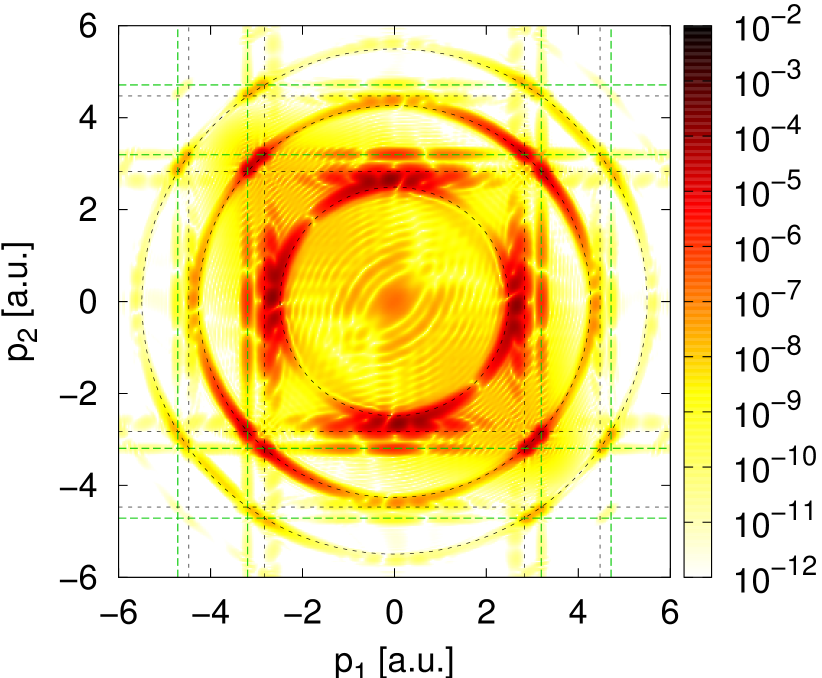
Figure 1: (Color online) Correlated photoelectron momentum spectrum calculated from the TDSE by applying a filter in position-space Wilken and Bauer (2007); Brics et al. (2014). A 7.6-nm 20-cycle $\sin^{2}$-shaped laser pulse of peak intensity $I_{0}=3.2\times 10^{15}\,\mathrm{W/cm^{2}}$ was used. The dashed green vertical and horizontal lines indicate the photoelectron momenta after single ionization of He by absorbing one and two photons. The dashed black vertical and horizontal lines indicate the photoelectron momenta after ionization of He⁺ by absorbing one and two photons.

SPDI is yet another effect where TDDFT does not work in practice, especially if one is interested in correlated photoelectron spectra, for which no density functional is known.

If $\hbar\omega>|E_{0}^{\mathrm{He}}|$ one photon can fully ionize a helium atom. However, electron-electron interaction is required in order to share the photon energy absorbed by one electron with another electron. From energy conservation, one obtains

$$E_{\mathrm{kin}}^{(1)}+E_{\mathrm{kin}}^{(2)}=\hbar\omega+E_{0}^{\mathrm{He}},$$ (32)

where $E_{\mathrm{kin}}^{(i)}$ is the kinetic energy of the $i$-th photoelectron. As a consequence, one expects a ring of radius $p=\sqrt{2\left(\hbar\omega+E_{0}^{\mathrm{He}}\right)}$ in correlated photoelectron momentum spectra. If both electrons are emitted in the same direction it is very improbable that one will measure both electrons with the same kinetic energy due to Coulomb repulsion. It is more likely that one electron will have a higher kinetic energy than the other. Thus, we expect the probability along the SPDI ring to vary. In fact, this is seen in Fig. 1. There is a minimum on the SPDI ring if both photoelectrons have the same energy and are emitted in the same direction.

An atom can simultaneously absorb also two and more photons. If $n$ is the number of photons which are simultaneously absorbed then the atom can be fully ionized if $n\hbar\omega>|E_{0}^{\mathrm{He}}|$. Thus, if the photon energy $\hbar\omega>|E_{0}^{\mathrm{He}}|$, rings of radii $p(n)=\sqrt{2\left(n\hbar\omega+E_{0}^{\mathrm{He}}\right)}$ with $n\in\left\{1,2,3,...\right\}$ are expected in correlated photoelectron momentum spectra. The probability to simultaneously absorb multiple photons decreases exponentially with the number of photons. Three rings can be identified in Fig. 1, and some traces of a fourth one. In order to observe more rings (within a dynamic range of ten orders of magnitude, as in Fig. 1) the laser intensity has to be increased.

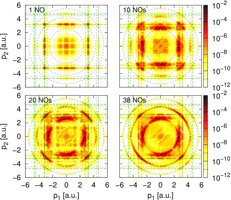
Figure 2: (Color online) Correlated photoelectron momentum spectra obtained from the first $i$ spatial NOs for $i=1,10,20,38$, calculated from the TDSE wavefunction at the end of pulse. Same laser pulse as in Fig. 1, dashed lines having same meaning.

The dashed vertical and horizontal lines in Fig. 1 indicate the expected photoelectron momenta after single ionization of He (green) and He⁺ (black) by one and two photons. An enhanced ionization probability is observed when dashed lines of different color cross the higher-order rings ($n=2,3,\ldots$), corresponding to sequential double ionization. The probability is smeared out due to electron-electron interaction, especially if the electrons are emitted in the same direction. The correlated photoelectron momentum spectra were calculated by applying a filter in position-space Wilken and Bauer (2007); Brics et al. (2014) instead of projecting out all bound and singly ionized states. As this is not a rigorous approach to calculate photoelectron spectra, traces of bound and singly excited states are still visible in Fig. 1.

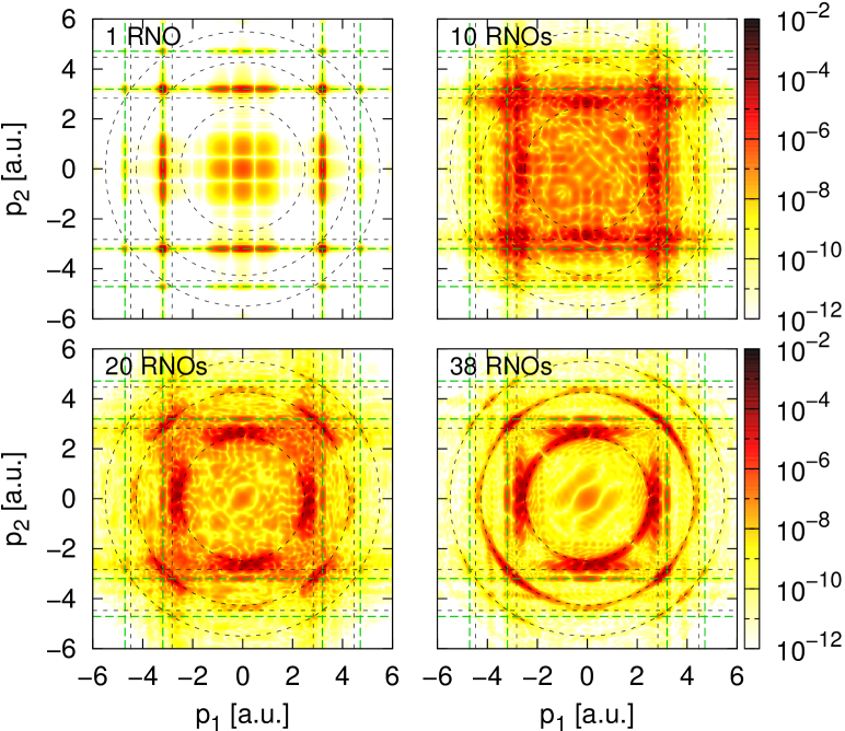
Figure 3: (Color online) Correlated photoelectron momentum spectra obtained by TDRNOT/MCTDHF with one to 38 spatial RNOs/determinants. Both methods yield exactly the same spectra when the same number of RNOs/determinants is used. Same laser pulse as in Fig. 1, dashed lines having same meaning.

To estimate the minimal number of spatial NOs or determinants required, one may take the first $N_{\circ}^{\mathrm{spat}}$ NOs with the highest ONs in (16), calculated from the exact TDSE wavefunction at the end of the laser pulse, to evaluate the observable of interest. Note that this corresponds to a hypothetical TDRNOT simulation without truncation error Rapp et al. (2014); Brics et al. (2014, 2016); Hanusch et al. (2016), i.e., with an infinite number of NOs taken into account for propagation, but only the dominating $N_{\circ}^{\mathrm{spat}}$ NOs used to calculate observables. Comparing Figs. 1 and 2 we find that $N_{\circ}^{\mathrm{spat}}=38$ NOs are required to accurately reproduce the SPDI ring $n=1$. $N_{\circ}^{\mathrm{spat}}\gg 1$ indicates that SPDI is a very correlated process, and differential, correlated photoelectron momentum spectra are correlation-sensitive observables. It is interesting to investigate how many RNOs for TDRNOT (or determinants in MCTDHF) are necessary to describe SPDI. In actual TDRNOT/MCTDHF calculations there is a truncation error so that it is expected that more NOs/determinants are needed to reproduce the correlated photoelectron spectra with TDRNOT/MCTDHF than in Fig. 2 where the NOs were calculated from the TDSE wavefunction. Such TDRNOT calculations of correlated photoelectron spectra in the context of nonsequential double ionization (NSDI) were pursued in Ref. Brics et al. (2014) where twice as many RNOs were found to be necessary for propagation to obtain similar results. TDRNOT/MCTDHF results for SPDI are shown in Fig. 3 for selected $N_{\circ}^{\mathrm{spat}}$ from 1 to 38. At 38, the major features of the correlated double-photoelectron spectrum are converged. Quite surprisingly, the convergence behavior is only slightly worse than that of the TDSE simulation when restricted to the respective $N_{\circ}^{\mathrm{spat}}$ in Fig. 2. Thus the truncation error does not play a crucial role for SPDI. This is probably because the laser pulses used for SPDI are of higher frequency and much shorter than in NSDI so that erroneously positioned and unphysical doubly excited states in the two-electron continuum Rapp et al. (2014) due to truncation play a minor part.

Table 1: Time (in seconds) required to calculate correlated photoelectron spectra for SPDI with TDRNOT, MCTDHF, and the TDSE. The calculations were performed on 4 cores of an i5-3570 processor using $N_{x}=1024$ grid points in each spatial direction.

$N_{\circ}^{\mathrm{spat}}$		11 TDRNOT 11	11MCTDHF11	11TDSE11	11 MCTDHF/TDRNOT 11	11 TDRNOT/TDSE 11
1	total time	0.82	1.29	46.99	1.6	0.02
	average $\Delta t$	0.0094	0.0093	0.05	1.0	0.19
10	total time	9.32	247.06	46.99	26.5	0.20
	average $\Delta t$	0.0079	0.0102	0.05	1.3	0.16
20	total time	51.80	6251.75	46.99	120.7	1.10
	average $\Delta t$	0.0053	0.0080	0.05	1.5	0.11
138 1	total time	467.69	190588.00	46.99	407.5	9.95
	1 average $\Delta t$ 1	0.0031	0.0058	0.05	1.9	0.06

IV.2 Computational effort

As already mentioned, any choice of the hermitian operator $\hat{g}(t)$ will lead to the same results (for a given number of RNOs/determinant) if one technically manages to solve the corresponding EOM. In practice, the simulations benefit from a gauge choice leading to EOM with good numerical properties. For instance, small matrix elements $g_{mn}(t)$ usually allow for larger time steps. Thus, by setting $g_{mn}(t)=0$, slightly larger average time steps can be used in MCTDHF than in TDRNOT, as visible from Table 1. However, comparing run times one finds that TDRNOT is nevertheless much faster. This is because the analytically known expansion coefficients $\gamma_{2,ijkl}(t)$ for a two-electron system form a sparse matrix in the NO basis but a dense one in MCTDHF. Hence, much less matrix elements need to be calculated in TDRNOT where for $2$-electron systems the numerically costly parts of the computations are found to scale as $\tau_{\mathrm{TDRNOT}}\sim N^{2}_{\circ}N_{t}N_{x}\log(N_{x})$ vs $\tau_{\mathrm{MCTDHF}}\sim N^{4}_{\circ}N_{t}N_{x}$. Here, $N_{x}$ denotes the number of grid points and $N_{t}$ the number of time steps (different gauges lead to different $\Delta t$ in adaptive propagation schemes). Note that in Refs. Brics et al. (2014, 2016) we reported that $\tau_{\mathrm{TDRNOT}}$ contains also a term $\sim N^{3}_{\circ}$. However, reduction to $\sim N_{\circ}^{2}$ is possible by calculating the sum over $p$ in $\mathbf{\mathcal{B}}_{nk}$ prior to the orbital scalar product, as indicated in (26). This comes at no additional cost since the EOM (23) requires $\sum_{k}\mathbf{\mathcal{\hat{C}}}_{nk}|\tilde{k}\rangle$ anyway.

The TDRNOT calculation with 38 RNOs is about 10 times slower than the TDSE. Hence, for the 1D model helium atom TDRNOT does not really offer computational gain. However, as $\tau_{\mathrm{TDSE}}\sim N_{t}N_{x}^{2}$ TDRNOT becomes superior with increasing $N_{x}$. Similarly, TDRNOT should be superior for simulations of He in full dimensionality. Unfortunately, it is still unclear if there is any computational gain in TDRNOT over MCTDHF for more than two-electrons. A crucial point here is whether available functionals for $\gamma_{2,ijkl}(t)$ such as the previously mentioned PNOF5e Piris et al. (2013) and PNOF6($N_{c}$) Lopez et al. (2015), which are exact in the 2-electron limit, perform well in practice for $N>2$.

V Conclusion

In this work, we tested further the recently introduced time-dependent renormalized-natural-orbital theory (TDRNOT) on single-photon double ionization (SPDI) of a numerically exactly solvable model helium atom. We showed how TDRNOT is related to multi-configurational time-dependent Hartree-Fock (MCTDHF). We also compared the performance of MCTDHF and TDRNOT, showing that TDRNOT is much faster. Unfortunately, the huge speedup over MCTDHF holds only for two-electron systems. The question whether there is any gain of using TDRNOT over MCTDHF for more-electron systems still needs to be answered and is subject of future work.

References

- Ullrich et al. (2003) J. Ullrich, R. Moshammer, A. Dorn, R. Dörner, L. P. H. Schmidt, and H. Schmidt-Böcking, “Recoil-ion and electron momentum spectroscopy: reaction-microscopes,” Reports on Progress in Physics 66, 1463 (2003).
- Berakdar et al. (2003) J. Berakdar, A. Lahmam-Bennani, and C. Dal Cappello, “The electron-impact double ionization of atoms: an insight into the four-body Coulomb scattering dynamics,” Physics Reports 374, 91 (2003).
- Ciappina et al. (2010) M. F. Ciappina, M. Schulz, and T. Kirchner, “Reaction dynamics in double ionization of helium by electron impact,” Phys. Rev. A 82, 062701 (2010).
- Amusia (2013) M. Y. Amusia, Atomic Photoeffect, Physics of Atoms and Molecules (Springer US, 2013).
- Byron and Joachain (1967) F. W. Byron and C. J. Joachain, “Multiple ionization processes in helium,” Phys. Rev. 164, 1 (1967).
- Førre (2012) M. Førre, “One-photon double ionization of helium: A heuristic formula for the cross section,” Phys. Rev. A 85, 013420 (2012).
- Lemell et al. (2015) C. Lemell, S. Neppl, G. Wachter, K. Tőkési, R. Ernstorfer, P. Feulner, R. Kienberger, and J. Burgdörfer, “Real-time observation of collective excitations in photoemission,” Phys. Rev. B 91, 241101 (2015).
- Brics and Bauer (2013) M. Brics and D. Bauer, “Time-dependent renormalized natural orbital theory applied to the two-electron spin-singlet case: Ground state, linear response, and autoionization,” Phys. Rev. A 88, 052514 (2013).
- Rapp et al. (2014) J. Rapp, M. Brics, and D. Bauer, “Equations of motion for natural orbitals of strongly driven two-electron systems,” Phys. Rev. A 90, 012518 (2014).
- Brics et al. (2014) M. Brics, J. Rapp, and D. Bauer, “Nonsequential double ionization with time-dependent renormalized-natural-orbital theory,” Phys. Rev. A 90, 053418 (2014).
- Brics et al. (2016) M. Brics, J. Rapp, and D. Bauer, “Strong-field absorption and emission of radiation in two-electron systems calculated with time-dependent natural orbitals,” Phys. Rev. A 93, 013404 (2016).
- Hanusch et al. (2016) A. Hanusch, J. Rapp, M. Brics, and D. Bauer, “Time-dependent renormalized-natural-orbital theory applied to laser-driven ,” Phys. Rev. A 93, 043414 (2016).
- Zanghellini et al. (2004) J. Zanghellini, M. Kitzler, T. Brabec, and A. Scrinzi, “Testing the multi-configuration time-dependent hartree-fock method,” J. Phys. B 37, 763 (2004).
- Caillat et al. (2005) J. Caillat, J. Zanghellini, M. Kitzler, O. Koch, W. Kreuzer, and A. Scrinzi, “Correlated multielectron systems in strong laser fields: A multiconfiguration time-dependent hartree-fock approach,” Phys. Rev. A 71, 012712 (2005).
- Hochstuhl et al. (2010) D. Hochstuhl, S. Bauch, and M. Bonitz, “Multiconfigurational time-dependent Hartree-Fock calculations for photoionization of one-dimensional Helium,” J. Phys. Conf. Ser. 220, 012019 (2010).
- Zielinski et al. (2016) A. Zielinski, V. P. Majety, and A. Scrinzi, “Double photoelectron momentum spectra of helium at infrared wavelength,” Phys. Rev. A 93, 023406 (2016).
- Ullrich (2011) C. A. Ullrich, Time-Dependent Density-Functional Theory: Concepts and Applications (Oxford University Press, Oxford, 2011).
- Ullrich and Yang (2013) C. A. Ullrich and Z.-H. Yang, “A brief compendium of time-dependent density functional theory,” Braz. J. Phys. 44, 154 (2013), arXiv:1305.1388.
- Wilken and Bauer (2007) F. Wilken and D. Bauer, “Momentum distributions in time-dependent density-functional theory: Product-phase approximation for nonsequential double ionization in strong laser fields,” Phys. Rev. A 76, 023409 (2007).
- Ruggenthaler and Bauer (2009) M. Ruggenthaler and D. Bauer, “Rabi Oscillations and Few-Level Approximations in Time-Dependent Density Functional Theory,” Phys. Rev. Lett. 102, 233001 (2009).
- Wilken and Bauer (2006) F. Wilken and D. Bauer, “Adiabatic Approximation of the Correlation Function in the Density-Functional Treatment of Ionization Processes,” Phys. Rev. Lett. 97, 203001 (2006).
- Coleman and Yukalov (2000) A. J. Coleman and V. I. Yukalov, Reduced Density Matrices: Coulson’s Challenge, Lecture Notes in Chemistry (Springer Berlin Heidelberg, Berlin, 2000).
- Appel (2007) H. Appel, Time-Dependent Quantum Many-Body Systems: Linear Response, Electronic Transport, and Reduced Density Matrices, Ph.D. thesis, Freie Universität Berlin, Berlin (2007), URN:nbn:de:kobv:188-fudissthesis000000003068-3.
- Giesbertz (2010) K. J. H. Giesbertz, Time-Dependent One-Body Reduced Density Matrix Functional Theory, Ph.D. thesis, Free University Amsterdam, Amsterdam (2010), URN:nbn:nl:ui:31-1871/16289.
- Lackner et al. (2015) F. Lackner, I. Březinová, T. Sato, K. L. Ishikawa, and J. Burgdörfer, “Propagating two-particle reduced density matrices without wave functions,” Phys. Rev. A 91, 023412 (2015).
- Lackner et al. (2017) F. Lackner, I. Březinová, T. Sato, K. L. Ishikawa, and J. Burgdörfer, “High-harmonic spectra from time-dependent two-particle reduced-density-matrix theory,” Phys. Rev. A 95, 033414 (2017).
- Ishikawa and Sato (2015) K. Ishikawa and T. Sato, “A review on ab initio approaches for multielectron dynamics,” IEEE J. Sel. Topics Quantum Electron. 21, 1 (2015).
- Hochstuhl et al. (2014) D. Hochstuhl, C. M. Hinz, and M. Bonitz, “Time-dependent multiconfiguration methods for the numerical simulation of photoionization processes of many-electron atoms,” Eur. Phys. J. Spec. Top. 223, 177 (2014).
- Greenman et al. (2010) L. Greenman, P. J. Ho, S. Pabst, E. Kamarchik, D. A. Mazziotti, and R. Santra, “Implementation of the time-dependent configuration-interaction singles method for atomic strong-field processes,” Phys. Rev. A 82, 023406 (2010).
- Pabst and Santra (2013) S. Pabst and R. Santra, “Strong-field many-body physics and the giant enhancement in the high-harmonic spectrum of xenon,” Phys. Rev. Lett. 111, 233005 (2013).
- Karamatskou et al. (2014) A. Karamatskou, S. Pabst, Y.-J. Chen, and R. Santra, “Calculation of photoelectron spectra within the time-dependent configuration-interaction singles scheme,” Phys. Rev. A 89, 033415 (2014).
- Bogoliubov (1946) N. N. Bogoliubov, “Kinetic equations,” J. Phys. USSR 10, 265 (1946).
- Bogoliubov and Gurov (1947) N. N. Bogoliubov and K. P. Gurov, “Kinetic equations in quantum mechanics,” J. Exp. Theor. Phys. (in Russian) 17, 614 (1947).
- Yvon (1935) J. Yvon, La Théorie Statistique des Fluides et l’Équation d’Etat, Actualités Scientifiques et Industrielles, Vol. 203 (Hermann, Paris, 1935).
- Kirkwood (1946) J. G. Kirkwood, “The statistical mechanical theory of transport processes i. general theory,” J. Chem. Phys. 14, 180 (1946).
- Kirkwood (1947) J. G. Kirkwood, “The statistical mechanical theory of transport processes ii. transport in gases,” J. Chem. Phys. 15, 72 (1947).
- Born and Green (1946) M. Born and H. S. Green, “A general kinetic theory of liquids. i. the molecular distribution functions,” Proceedings of the Royal Society of London A: Mathematical, Physical and Engineering Sciences 188, 10 (1946).
- Piris et al. (2013) M. Piris, J. M. Matxain, and X. Lopez, “The intrapair electron correlation in natural orbital functional theory,” J. Chem. Phys. 139, 234109 (2013).
- Lopez et al. (2015) X. Lopez, M. Piris, F. Ruipérez, and J. M. Ugalde, “Performance of PNOF6 for hydrogen abstraction reactions,” J. Phys. Chem. A 119, 6981 (2015).
- Meyer et al. (1990) H.-D. Meyer, U. Manthe, and L. S. Cederbaum, “The multi-configurational time-dependent Hartree approach,” Chem. Phys. Lett. 165, 73 (1990).
- Manthe et al. (1992) U. Manthe, H.-D. Meyer, and L. S. Cederbaum, “Wave-packet dynamics within the multiconfiguration Hartree framework: General aspects and application to NOCl,” J. Chem. Phys. 97, 3199 (1992).
- Jansen (1993) A. P. J. Jansen, “A multiconfiguration time-dependent Hartree approximation based on natural single-particle states,” J. Chem. Phys. 99, 4055 (1993).
- Manthe (1994) U. Manthe, “Comment on ‘A multiconfiguration time-dependent Hartree approximation based on natural single-particle states‘ [J. Chem. Phys. 99, 4055 (1993)],” J. Chem. Phys. 101, 2652 (1994).
- Sato and Ishikawa (2014) T. Sato and K. L. Ishikawa, “The structure of approximate two electron wavefunctions in intense laser driven ionization dynamics,” J. Phys. B 47, 204031 (2014).
- Scrinzi (2010) A. Scrinzi, “Infinite-range exterior complex scaling as a perfect absorber in time-dependent problems,” Phys. Rev. A 81, 053845 (2010).
- Grobe and Eberly (1992) R. Grobe and J. H. Eberly, “Photoelectron spectra for a two-electron system in a strong laser field,” Phys. Rev. Lett. 68, 2905 (1992).
- Haan et al. (1994) S. L. Haan, R. Grobe, and J. H. Eberly, “Numerical study of autoionizing states in completely correlated two-electron systems,” Phys. Rev. A 50, 378 (1994).
- Bauer (1997) D. Bauer, “Two-dimensional, two-electron model atom in a laser pulse: Exact treatment, single-active-electron analysis, time-dependent density-functional theory, classical calculations, and nonsequential ionization,” Phys. Rev. A 56, 3028 (1997).
- Lappas and van Leeuwen (1998) D. G. Lappas and R. van Leeuwen, “Electron correlation effects in the double ionization of He,” J. Phys. B 31, L249 (1998).
- Lein and Kümmel (2005) M. Lein and S. Kümmel, “Exact time-dependent exchange-correlation potentials for strong-field electron dynamics,” Phys. Rev. Lett. 94, 143003 (2005).
- Dormand and Prince (1980) J. R. Dormand and P. J. Prince, “A family of embedded Runge-Kutta formulae,” J. Comput. Appl. Math. 6, 19 (1980).