$XMM$-$Newton$ and $NuSTAR$ simultaneous X–ray observations of IGR J11215-5952

Abstract

We report the results of an $XMM$-$Newton$  and $NuSTAR$ coordinated observation of the Supergiant Fast X–ray Transient (SFXT) IGR J11215–5952, performed on February 14, 2016, during the expected peak of its brief outburst, which repeats every $\sim$165 days. Timing and spectral analysis were performed simultaneously in the energy band 0.4–78 keV. A spin period of 187.0 ($\pm{0.4}$) s was measured, consistent with previous observations performed in 2007. The X–ray intensity shows a large variability (more than one order of magnitude) on timescales longer than the spin period, with several luminous X–ray flares which repeat every 2-2.5 ks, some of which simultaneously observed by both satellites. The broad-band (0.4-78 keV) time-averaged spectrum was well deconvolved with a double-component model (a blackbody plus a power-law with a high energy cutoff) together with a weak iron line in emission at 6.4 keV (equivalent width, EW, of 40$\pm{10}$ eV). Alternatively, a partial covering model also resulted in an adequate description of the data. The source time-averaged X–ray luminosity was 10³⁶ erg s^-1 (0.1-100 keV; assuming 7 kpc). We discuss the results of these observations in the framework of the different models proposed to explain SFXTs, supporting a quasi-spherical settling accretion regime, although alternative possibilities (e.g. centrifugal barrier) cannot be ruled out.

1. Introduction

The last decade has witnessed an important advance in understanding high mass X–ray binaries (HMXBs), thanks to the discovery of Supergiant Fast X–ray Transients (SFXTs; Sguera et al. 2005; Negueruela et al. 2005) during INTEGRAL (Winkler et al., 2003, 2011) monitoring observations of the Galactic plane at hard X–ray energies, above 20 keV.

SFXTs are celestial objects characterized by outbursts of brief duration (with the brightest phase typically concentrated in one day) made of a sequence of luminous X–ray flares (normally reaching 10³⁶-10³⁷ erg s^-1), each flare lasting a few thousand seconds at most. SFXTs are associated with early-type supergiants, making them a subclass of HMXBs. Their X–ray properties were quickly recognized as a challenge to the accretion models: apparently, SFXTs share similar properties (donor spectral type, orbital geometry, neutron star spin periods) to classical persistent HMXBs hosting supergiant stars, except for their extremely variable X–ray behaviour (see, e.g., Sidoli 2013; Walter et al. 2015).

Their bright X–ray flares are typically sporadic and rare, occurring with a very low duty cycle which ranges from 0.01% to 5% at most (Paizis & Sidoli, 2014). The time-averaged X–ray luminosity is below 10³⁴ erg s^-1 (Sidoli et al., 2008; Bozzo et al., 2015).

Although some SFXTs with measured orbital periods show outbursts more frequently near periastron, the occurrence of an SFXT flare in most cases cannot be predicted. The exception is IGR J11215–5952, which is the only source of the class that undergoes outbursts periodically (Sidoli et al., 2006), every $\sim$165 days (Sidoli et al., 2007; Romano et al., 2009). This periodicity is interpreted as due to the orbital period of the system. Sidoli et al. (2007) suggested that its clocked and brief outbursts are produced by enhanced accretion when the neutron star of the system crosses the focussed outflowing wind along a plane inclined with respect to the orbit near periastron passage.

Its optical counterpart, HD 306414, is a B0.5 Ia star, located at a distance $d\gtrsim 7\>$kpc (Lorenzo et al., 2014). The high resolution optical spectroscopy suggests a high orbital eccentricity (e$>$0.8, Lorenzo et al. 2014). IGR J11215–5952 is also an X–ray pulsar (P_spin=187 s; Swank et al. 2007), a property which makes this SFXT a laboratory to unveil the accretion mechanism driving the SFXT behaviour.

In this paper, we report on an $XMM$-$Newton$ observation coordinated with $NuSTAR$ of IGR J11215–5952 performed in February 2016, aimed at investigating the broad-band spectrum searching for cyclotron absorption lines, to directly measure the neutron star magnetic field, and disentangle between competing models proposed to explain the X-ray behaviour of SFXTs. A monitoring with $Swift$ allowed us to place these observations within the context of the whole outburst. We assume a source distance of 7 kpc (Lorenzo et al., 2014).

2. Observations and Data Reduction

2.1. $XMM$-$Newton$

The $XMM$-$Newton$ $Observatory$ (Jansen et al., 2001) carries three X–ray telescopes, each with an European Photon Imaging Camera (EPIC; 0.4-12 keV) at the focus: two with MOS CCDs (Turner et al., 2001) and one with a pn CCD (Strüder et al., 2001). Reflection Grating Spectrometer (RGS; 0.4-2.1 keV) arrays (den Herder et al., 2001) are placed at two of the telescopes.

The $XMM$-$Newton$ observation targeted on IGR J11215–5952 started on 2016 February 14 at 21:25 and ended the day after at 03:36, resulting in net exposure times of 22 ks and 15.5 ks for the MOS and the pn, respectively. All EPIC cameras were operated in small window mode and adopted the medium filter.

We reduced the data using version 15.0.0 of the Science Analysis Software (SAS) with standard procedures and the most updated calibration files. We used the HEASoft version 6.18 to perform the data analysis.

At first, we extracted EPIC source counts from circular regions of 30^′′ radius, adopting PATTERN selection from 0 to 4 in the pn and from 0 to 12 in MOS spectra. We evaluated the possible presence of pile-up in EPIC data with epatplot, finding moderate pile-up only in MOS data. This suggested to excise the core of the PSF in both MOS data, extracting MOS1 and MOS2 spectra from annular regions with inner radius of 5^′′and an outer radius of 30^′′. Background spectra were obtained from similar sized regions offset from the source positions. The full exposure time was exploited and no further filtering was applied to the data.

The SAS task rgsproc was used to extract the RGS1 and RGS2 spectra, which were later combined into one single grating spectrum using rgscombine present in the SAS.

Appropriate response matrices were generated using the SAS tasks arfgen and rmfgen. EPIC spectra were analysed in the energy range 0.4-12, while the RGSs, which operated in spectroscopy mode (den Herder et al., 2001), were analysed in the range 0.4-2.1 keV.

To ensure applicability of the $\chi^{2}$ statistics, the spectra were rebinned such that at least 20 counts per bin were present. Free relative normalizations between the spectra were included to account for uncertainties in instrumental responses, always fixing at 1 the normalization of the EPIC pn spectrum. Spectral uncertainties are given at 90% confidence for one interesting parameter.

In the spectral fitting we used the photoelectric absorption model TBabs in xspec adopting the interstellar abundances of Wilms et al. (2000) and photoelectric absorption cross-sections by Balucinska-Church & McCammon (1992).

The final, time-averaged, source net count rates were the following: 5.67$\pm{0.02}$ counts s^-1 (EPIC pn), 1.143$\pm{0.007}$ counts s^-1 (MOS1, PSF core excised), 1.130$\pm{0.007}$ counts s^-1 (MOS2, PSF core excised), 0.027$\pm{0.001}$ counts s^-1 (combined RGS1 and RGS2 1st order spectra).

The high absorption towards the source (column density, N_H, around 10²² cm^-2) implied significant detection in the RGSs only above 1 keV. This limited the available RGS band to the range 1-2 keV. The low statistics leave us with an apparent featureless RGS spectrum. Therefore we will not discuss it further in the paper.

2.2. $NuSTAR$

IGR J11215–5952 was observed by $NuSTAR$ as part of the joint $XMM$-$Newton$/$NuSTAR$ programme approved during $XMM$-$Newton$ Announcement of Opportunity AO14, with the main aim of searching for cyclotron lines.

$NuSTAR$ observations started on 2016 February 14 at 17:11 and ended the day after at 05:01, for a net exposure time of 20.3 ks.

The Nuclear Spectroscopic Telescope Array ($NuSTAR$, Harrison et al. 2013) is the first focusing hard X-ray telescope above 10 keV and was launched in 2012. It carries two identical co-aligned telescopes that focus X-ray photons onto two independent Focal Plane Modules, called A and B (hereafter FPMA and FPMB). Each FPM contains four (2$\times$2) solid-state cadmium zinc telluride (CdZnTe) pixel detectors which provide a spatial resolution of 18^′′ (full width at half maximum, FWHM), a spectral resolution of 400 eV (FWHM) at 10 keV, and a 12^′$\times$12^′ field-of-view (FOV). The effective area is calibrated in the energy range 3-78 keV (Madsen et al., 2015). The low satellite orbit (with a $\sim$90 minute period) produces data-gaps lasting about 30 minutes every orbit in the $NuSTAR$ observations.

We processed $NuSTAR$ data (obsID 30101008002) with the version 1.5.1 (2015, June 9) of the $NuSTAR$ data analysis software ($NuSTAR~{}DAS$), using CALDB version 20150316. Spectra and lightcurves were extracted with nuproducts on the cleaned event files. Circular extraction regions with a 60^′′ radius were used around IGR J11215–5952 and for the background, well away from the point-spread function (PSF) source wings. $NuSTAR$ observation was not contaminated by any stray-light produced by sources outside the FOV. Since the background was stable and constant along the observation, no further filtering was applied. $NuSTAR$ source light curves with arrival times corrected to the Solar System barycenter have been extracted with the $NuSTAR~{}DAS$ tool nuproducts and “barycorr=yes”. When needed, good-time intervals (GTIs) were generated using xselect and then running nuproducts using the “usrgtifile” keyword, to correctly extract the temporal selected spectra.

The source net count rates were the following (3-78 keV): 1.783$\pm{0.009}$ counts s^-1 (FPMA) and 1.678$\pm{0.009}$ counts s^-1 (FPMB). Spectra were rebinned in order to have at least 20 counts per bin to ensure the applicability of the $\chi^{2}$ statistics. Spectra from FPMA and FPMB were simultaneously fitted in xspec, without merging them together. Cross-calibration constants were used during the spectral analysis to take into account calibration uncertainties.

The same procedure was used when $XMM$-$Newton$ and $NuSTAR$ spectra were jointly fitted together.

2.3. $Swift$

After acceptance of the joint $XMM$-$Newton$/$NuSTAR$ AO14 observations, we asked for a monitoring with $Swift$ around 2016, February 14. Five snapshots (2 ks duration each), from 2016, February 11 to February 19 were performed, with the main aim of monitoring the source light curve to put the $XMM$-$Newton$ and $NuSTAR$ IGR J11215–5952 intensity into context of the outburst evolution.

The $Swift$/XRT source light curve (Fig. 1, upper panel) was built making use of the XRT data products generator available at the UK $Swift$ Science Data Centre (Evans et al., 2007).

Figure 1.— IGR J11215–5952 light curves during the 2016 February outburst, observed by three different satellites: $Swift$/XRT (PC mode, 0.3-10 keV), $NuSTAR$ (FPMA, 3-78 keV) and $XMM$-$Newton$ (EPIC pn, 0.4-12 keV). Time is in units of seconds from the first $Swift$/XRT observation performed on February 11.

3. Analysis and Results

3.1. Light curves

In Fig. 1 we show the source light curve observed by $Swift$, $NuSTAR$ and $XMM$-$Newton$  during the outburst. In particular, the $Swift$ monitoring demonstrates that both $NuSTAR$ and $XMM$-$Newton$ observations caught the transient at its peak, as expected.

In Fig. 2 we show only the light curves as observed by $XMM$-$Newton$ (EPIC pn, 0.4-12 keV) and $NuSTAR$ (FPMA, for clarity, 3-78 keV) binned on the known spin (187 s, see below), to avoid variability due to the neutron star rotational period. The intensity variability is large, in excess of one order of magnitude. The uninterrupted $XMM$-$Newton$ light curve clearly shows that each satellite gap in the NuSTAR observation is actually filled by bright flares, repeating on a timescale of 2-2.5 ks.

Figure 2.— IGR J11215–5952 light curve during the February 2016 outburst observed by EPIC pn (upper panel; 0.4–12 keV) and $NuSTAR$ FPMA (lower panel; 3-78 keV). The bin time is 187 s which is its pulsation period. Numbers indicate the sequence of flares in $NuSTAR$ observation (same numbers used in the temporal-selected spectroscopy). The small horizontal lines under the numbers approximately indicate the exposure times of each flare spectrum.

We performed timing analysis on EPIC (all three cameras, 2-12 keV) and $NuSTAR$ data (FPMA and FPMB, 3-78 keV) after correcting arrival times to the Solar System barycenter, applying epoch folding techniques (Leahy et al., 1983) to measure the known neutron star spin period. We determined a periodicity of 187.0$\pm{0.4}$ s, consistent with what observed in 2007 with $XMM$-$Newton$ (Sidoli et al., 2007) and with $RXTE$/PCA (Swank et al., 2007).

In Fig. 3 we show the pulse profiles extracted from the strictly simultaneous $XMM$-$Newton$ and $NuSTAR$ data, in different energy ranges, together with four hardness ratios. The pulse profile is energy dependent, being dominated by an asymmetric main peak below 12 keV, which becomes symmetric at harder energies. The hardness ratios display different behavior along the pulse phase, as show in the lower panels in Fig.3.

The pulsed fraction, PF, calculated as $PF\equiv(F_{\rm{max}}-F_{\rm{min}})/(F_{\rm{max}}+F_{\rm{min}})$, where F_max and F_min are the count rates at the maximum and at the minimum of the pulse profile, respectively, increases with energy, from $24\pm{3}$ % (0.4-3 keV) to $60\pm{14}$ % (20-78 keV). Over the whole $XMM$-$Newton$ energy band PF=$26\pm{2}$ % (0.4-12 keV), while PF=$29\pm{3}$ % over the whole $NuSTAR$ band (3-78 keV).

Figure 3.— IGR J11215–5952 pulse profiles (period P=187 s; MJD 57432 is the epoch of $\phi$=0) in different energy ranges are shown, as observed simultaneously by $XMM$-$Newton$ (EPIC pn, left panels) and by NuSTAR (FPMA for clarity, right panels). Four hardness ratios are displayed, calculated in the following energy ranges: HR1=(3-6 keV)/(0.4-3 keV); HR2=(6-12 keV)/(3-6 keV); HR3=(12-20 keV)/(6-12 keV); HR4=(20-78 keV)/(12-20 keV).

3.2. Spectra

3.2.1 Time-averaged $XMM$-$Newton$ and $NuSTAR$ spectrum

We extracted $NuSTAR$ spectra overlapping in time with the whole $XMM$-$Newton$ observation, to investigate the broad-band (0.4-78 keV) time-averaged IGR J11215–5952 emission. This translated into a net exposure time of $\sim$9 ks for each $NuSTAR$ FPM.

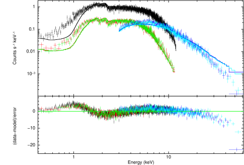
Figure 4.— Time-average broad-band spectrum, using EPIC and $NuSTAR$ data. Count spectra are shown together with the residuals (in units of standard deviation) with respect to a simple absorbed power law, to clearly show the structures in the residuals. EPIC spectra are marked in black (pn), red (MOS1) and green (MOS2) colors, $NuSTAR$ spectra in blue (FPMA) and in pale blue (FPMB).

The joint fit of the five spectra (EPIC pn, MOS1, MOS2, FPMA and FPMB) with a single absorbed power-law model provided unacceptable results ($\chi^{2}_{\nu}$=2.89 for 3292 degrees of freedom, dof; Fig. 4), because of an evident rollover at hard energies, together with a soft excess (below 1.5 keV) and positive residuals at $\sim$6.4 keV, consistent with a K_α emission line from neutral iron. We tried different double-component continuum models. The best-fit was obtained adopting a blackbody (with a temperature, kT_BB, of $\sim$1.6 keV, and a radius, ${\rm R_{BB}}$, of a few hundred meters, calculated assuming a distance of 7 kpc), together with a hard power-law (photon index, $\Gamma$, of 0.6) modified by a cut-off at high energy (hereafter PLCUT), defined as M(E)=${(exp[(E_{cut}-E)/E_{fold}])}$ when E$\geq E_{cut}\>$, while M(E)=1 at E$\leq E_{cut}\>$. An additive Gaussian line in emission around 6.4 keV was also needed. The results are reported in Table LABEL:tab:av_spec (Model 1) and shown in Fig. 5. The presence of a blackbody component was already known from previous $XMM$-$Newton$ observations of IGR J11215-5952 performed in 2007 (Sidoli et al., 2007) and it usually accounts for soft excesses detected in several accreting pulsars (La Palombara & Mereghetti, 2006). We also tried an alternative decomposition of the broad-band spectrum, replacing the blackbody component with a partial covering fraction absorption (pcfabs model in xspec). This model consists of an additional intrinsic absorption (N_Hpcfabs) with a covering fraction f_pcfabs (${\rm 0<f_{\rm pcfabs}<1}$), so that the continuum is:

$${\rm Intensity=e^{-\sigma N_{H}}\;[fe^{-\sigma N_{Hpcfabs}}\rm+\;(1-\;f)]\;(I_{PLCUT}),}$$

A partially covered PLCUT model (hereafter Model 2) provided an equivalently good description of the data.

Note that consistent spectral results were obtained from strictly simulataneous $XMM$-$Newton$ and $NuSTAR$ time-averaged spectra, but we considered here the whole $XMM$-$Newton$ exposure time to better constrain the parameters of the iron emission line.

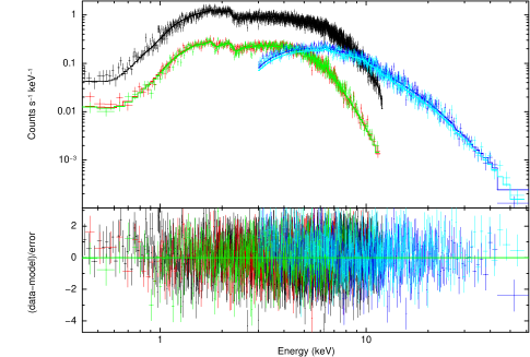
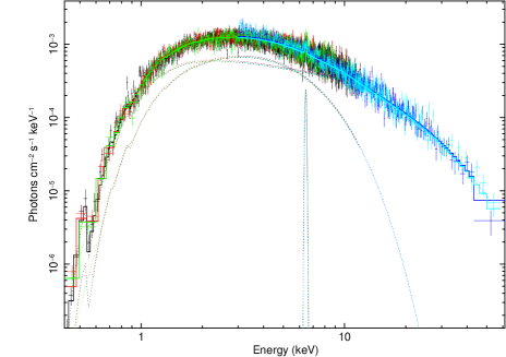
Figure 5.— Time-average broad-band spectrum, using EPIC and $NuSTAR$ data (only events overlapping in time with the $XMM$-$Newton$ observation, as discussed in Sect. 3.2.1). Count spectra are shown on the left together with the residuals (in units of standard deviation) with respect to the best-fit model reported in Table LABEL:tab:av_spec. Photon spectra are displayed on the right. EPIC spectra are marked in black (pn), red (MOS1) and green (MOS2) colors, $NuSTAR$ spectra in blue (FPMA) and in pale blue (FPMB).

Table 1Broad-band time-averaged spectrum (0.4–78 keV).

Parameter	Model 1	Model 2
NH ($10^{22}$ cm-2)	$1.05\pm{0.06}$	$1.27^{+0.07}_{-0.09}$
NHpcfabs ($10^{22}$ cm-2)	none	$4.5^{+0.6}_{-0.9}$
fpcfabs	none	$0.51\pm{0.04}$
kTBB (keV)	$1.61^{+0.06}_{-0.07}$	none
${\rm R_{BB}}$ (m)	$460\pm{30}$	none
$\Gamma$a	$0.56^{+0.08}_{-0.11}$	$0.97^{+0.11}_{-0.08}$
Ecut (keV)	$9.7^{+0.9}_{-1.0}$	$5.5^{+0.8}_{-0.4}$
Efold (keV)	$14.3\pm{1.4}$	$15.3^{+1.8}_{-1.4}$
Eline (keV)	$6.44^{+0.03}_{-0.03}$	$6.45^{+0.03}_{-0.03}$
$\sigma$line (keV)	$<0.09$	$<0.09$
Fluxline (ph cm-2 s-1)	($3.2\pm{0.8}$)$\times 10^{-5}$	($3.2^{+0.9}_{-0.4}$)$\times 10^{-5}$
EWlineb (eV)	$40\pm{10}$	$41^{+12}_{-5}$
Fluxc (erg cm-2 s-1)	(1.7$\pm{0.1}$) $\times$10-10	(1.8$\pm{0.1}$) $\times$10-10
Luminosityc (erg s-1)	(1.0$\pm{0.1}$) $\times$1036	(1.1$\pm{0.1}$) $\times$1036
$\chi^{2}_{\nu}$/dof	1.042/3285	1.057/3285

3.2.2 Temporal-selected spectroscopy

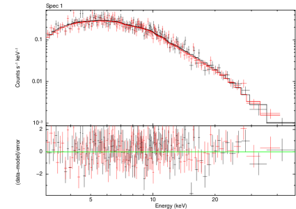
Figure 6.— $NuSTAR$ temporal-selected spectroscopy (FPMA in black, FPMB in red) of the peak of flare n. 1. Counts spectrum is shown (together with the residuals), fitted with an absorbed PLCUT model (Table LABEL:tab:revsel).

Cyclotron resonant scattering features (CRSFs) in X–ray pulsars with standard neutron star magnetic fields (a few $10^{12}$ Gauss) can be detected in the X–ray spectrum at energies E$>$10 keV. Thus, in principle, if they are strong enough also in IGR J11215–5952  they should be found in the $NuSTAR$ spectra alone. Therefore, we started concentrating on $NuSTAR$ data only, extracting spectra from the peaks of the flares, as shown in Fig. 2 (numbers in the lower panel).

When fitting $NuSTAR$ data only, the soft blackbody component that was evident in the broad-band time-averaged spectrum (Sect. 3.2.1) could not be constrained, as well as the absorption column density and the iron emission line (this latter is evident only in the time-averaged spectrum). Since we were interested in searching for absorption features at hard energies (E$>$10 keV), we preferred not to include the blackbody component and the iron line in the spectral model. The absorbing column density was a free parameter in the fit. In this manner, it naturally converged to very high (and unrealistic) values, with respect to the time-averaged spectroscopy of $XMM$-$Newton$ and $NuSTAR$ simultaneous data. As a first attempt, we simply adopted this absorbed PLCUT model as a pure phenomenological and statistically acceptable description of the continuum emission. The results from fitting the eight time-resolved 3-78 keV spectra in this way are reported in Table LABEL:tab:revsel.

Table 2Time-resolved spectroscopy (3–78 keV), fitting only $NuSTAR$ data of the flare peaks.

Parameter	Spec. 1	2	3	4	5	6	7	8
NH ($10^{22}$ cm-2)	$7^{+5}_{-4}$	$8\pm{3}$	$6\pm{3}$	$5^{+6}_{-5}$	$9\pm{4}$	$9\pm{4}$	$5^{+6}_{-5}$	$3^{+6}_{-3}$
$\Gamma$	$1.4^{+0.5}_{-0.3}$	$1.6^{+0.2}_{-0.2}$	$1.04^{+0.22}_{-0.22}$	$1.27^{+0.37}_{-0.30}$	$1.69^{+0.15}_{-0.61}$	$1.64^{+0.11}_{-0.10}$	$1.6^{+0.4}_{-0.7}$	$1.28^{+0.19}_{-0.60}$
Ecut (keV)	$6\pm{6}$	$7^{+3}_{-2}$	$3^{+4}_{-3}$	$7^{+5}_{-7}$	$15^{+8}_{-15}$	$22^{+13}_{-3}$	$9^{+14}_{-9}$	$8^{+5}_{-8}$
Efold (keV)	$27^{+35}_{-8}$	$33^{+20}_{-13}$	$15^{+5}_{-3}$	$25^{+22}_{-8}$	$40^{+50}_{-20}$	$19^{+28}_{-19}$	$30^{+40}_{-12}$	$20^{+9}_{-9}$
F (10-10 erg cm-2 s-1)a	3.0$\pm{0.3}$	3.6$\pm{0.4}$	2.5$\pm{0.2}$	3.2$\pm{0.3}$	4.6$\pm{0.3}$	3.1$\pm{0.2}$	2.3$\pm{0.7}$	1.7$\pm{0.2}$
L (1036 erg s-1) a	1.8$\pm{0.2}$	2.1$\pm{0.2}$	1.5$\pm{0.1}$	1.9$\pm{0.2}$	2.7$\pm{0.2}$	1.8$\pm{0.1}$	1.3$\pm{0.4}$	1.1$\pm{0.1}$
$\chi^{2}_{\nu}$/dof	1.046/239	0.949/347	0.998/282	1.121/155	0.900/164	0.887/160	0.602/89	0.839/94

Table 3Same as Table LABEL:tab:revsel ($NuSTAR$ only), considering only flare peaks 1,2,3,4 and 6, where the inclusion of an absorption feature resulted in a line significance larger than 2 $\sigma$.

Parameter	Spec. 1	2	3	4	6
NH ($10^{22}$ cm-2)	$10\pm{3}$	$7^{+4}_{-7}$	$6\pm{4}$	$4^{+6}_{-4}$	$6^{+4}_{-4}$
$\Gamma$	$1.6^{+0.2}_{-0.2}$	$1.40^{+0.19}_{-1.39}$	$1.4^{+0.3}_{-0.4}$	$1.15^{+0.31}_{-0.32}$	$1.49^{+0.14}_{-0.14}$
Ecut (keV)	$19^{+4}_{-9}$	$6.3^{+2.2}_{-6.3}$	$7^{+4}_{-7}$	$6.4^{+1.8}_{-6.4}$	$20^{+3}_{-3}$
Efold (keV)	$21^{+21}_{-8}$	$27^{+16}_{-13}$	$31^{+95}_{-15}$	$23^{+12}_{-7}$	$15^{+9}_{-5}$
Depthcycla	$0.44^{+0.18}_{-0.17}$	$0.16^{+0.16}_{-0.11}$	$0.74^{+2.9}_{-0.46}$	$0.38^{+0.31}_{-0.26}$	$0.46^{+0.27}_{-0.25}$
Ecycla (keV)	$16.7^{+1.0}_{-0.9}$	$15^{+3}_{-5}$	$32.5^{+4.2}_{-3.4}$	$18.0\pm{1.0}$	$17.2\pm{0.7}$
Widthcycla (keV)	$2.6^{+3.2}_{-1.5}$	$1.6^{+14}_{-1.6}$	$4.9^{+11.3}_{-4.9}$	$1.0^{+2.4}_{-1.0}$	$1.0^{+1.2}_{-1.0}$
Line Signif.b	4.4 $\sigma$	2.3 $\sigma$	2.7 $\sigma$	2.5 $\sigma$	3.25 $\sigma$
$\chi^{2}_{\nu}$/dof	1.012/236	0.942/344	0.984/279	1.103/152	0.837/157

In some of these spectra, negative residuals appeared at energies between 15 and 40 keV. To account for these absorption features, we modified the PLCUT continuum multiplying it with a cyclotron absorption model (cyclabs in xspec package). At first, we calculated the line significance by increasing the $\Delta\chi^{2}$ value until the confidence region boundary of the depth (Depth_cycl in Table LABEL:tab:revsel_cyclabs) of the cyclotron line crosses 0. The significance of these lines was greater than 2$~{}\sigma$ in five (of eight) spectra (flares number 1, 2, 3, 4 and 6), so we have reported absorption line parameters only for these spectra in Table LABEL:tab:revsel_cyclabs for clarity. The absorption lines were measured with a significance ranging from $\sigma$=2.3 to $\sigma$=4.4 (with cyclabs model), with the best value obtained during the first flare observed by $NuSTAR$. The centroid energy was different: in spectra n. 1, 4 and 6 the feature was in a narrow range around 17-18 keV, while during spectrum n. 3 it was at $\sim$33 keV. In spectrum n. 3 the line at $\sim$17 keV was undetected: we could place an upper limit (Depth_cycl$\lesssim 0.18\>$) to the depth of the cyclabs line with the centroid energy fixed at 17 keV (and line width of 2 keV).

In order to test the significance of the absorption line, since the F-test could bring unreliable results (Protassov et al., 2002), we exploited Monte Carlo simulations to confirm the presence of the cyclotron line in spectrum n.1 (our best case, Fig. 6), following the approach described by several authors (Bhalerao et al., 2015; Lotti et al., 2016; Barrière et al., 2015). We used the simftest routine in xspec with 100000 simulations, fixing the $N_{\rm H}$ to the values reported in Table LABEL:tab:revsel_cyclabs to speed up the process, and found that the probability of such line to be required by the data is $P=99.15\%$ for spectrum n. 1, corresponding to $2.63$ $\sigma$ (normalized to 8 trials). The significance of the line did not improve if a blackbody component was included in the fitting model to flare n.1 spectrum, with a temperature, radius and absorption fixed to the broad-band time-averaged values.

Table 4Broad-band (0.4-78 keV) spectroscopy of the flares simultaneously observed by $XMM$-$Newton$ and $NuSTAR$.

Model 1a Parameters	flare 4	4	5	6	6	7
NH ($10^{22}$ cm-2)	$1.08^{+0.28}_{-0.29}$	$0.94^{+0.31}_{-0.30}$	$0.89^{+0.25}_{-0.24}$	$1.15^{+0.21}_{-0.20}$	$1.00^{+0.24}_{-0.24}$	$1.3^{+0.1}_{-0.1}$
kTBB (keV)	$1.68^{+0.43}_{-0.22}$	$1.47^{+0.27}_{-0.18}$	$1.51^{+0.39}_{-0.16}$	$1.88^{+0.13}_{-0.10}$	$1.71^{+0.15}_{-0.12}$	$1.94^{+0.07}_{-0.07}$
${\rm R_{BB}}$ (m)	$480^{+180}_{-120}$	$600^{+250}_{-160}$	$630^{+200}_{-120}$	$450^{+60}_{-50}$	$520^{+90}_{-80}$	$380^{+10}_{-10}$
$\Gamma$	$0.54^{+0.23}_{-0.36}$	$0.29^{+0.31}_{-0.94}$	$0.43^{+0.25}_{-0.40}$	$0.85^{+0.13}_{-0.14}$	$0.64^{+0.19}_{-0.29}$	$1.11^{+0.05}_{-0.05}$
Ecut (keV)	$6\pm{6}$	$6.4^{+1.2}_{-1.6}$	$7^{+11}_{-7}$	$21^{+2.5}_{-2.2}$	$18.6^{+2.3}_{-3.2}$	$29^{+3}_{-2}$
Efold (keV)	$15^{+6}_{-4}$	$12^{+4}_{-4}$	$13^{+5}_{-3}$	$12^{+7}_{-4}$	$9.9^{+3.5}_{-2.5}$	$<25$
Depthcycl	none	$0.45^{+0.30}_{-0.28}$	none	none	$0.64^{+0.32}_{-0.33}$	none
Ecycl (keV)	none	$18.1^{+1.0}_{-1.8}$	none	none	$17.4^{+0.64}_{-0.67}$	none
Widthcycl (keV)	none	$1^{+4}_{-1}$	none	none	$1^{+1.4}_{-1}$	none
Line Signif.b	none	2.8 $\sigma$	none	none	3.35 $\sigma$	none
F (10-10 erg cm-2 s-1)c	2.8$\pm{0.4}$	2.8$\pm{0.4}$	3.1$\pm{0.4}$	2.4$\pm{0.2}$	2.4$\pm{0.2}$	1.6$\pm{0.1}$
L (1036 erg s-1) c	1.6$\pm{0.2}$	1.6$\pm{0.4}$	1.8$\pm{0.2}$	1.4$\pm{0.1}$	1.4$\pm{0.1}$	0.94$\pm{0.06}$
$\chi^{2}_{\nu}$/dof	0.989/457	0.978/454	1.018/503	0.869/492	0.851/489	0.929/271
Model 2a Parameters	flare 4	4	5	6	6	7
NH ($10^{22}$ cm-2)	$1.47^{+0.28}_{-0.38}$	$1.37^{+0.30}_{-0.42}$	$1.30^{+0.28}_{-0.43}$	$1.37^{+0.24}_{-0.26}$	$1.6^{+0.2}_{-0.2}$	$1.52^{+0.38}_{-0.79}$
NHpcfabs ($10^{22}$ cm-2)	$8\pm{4}$	$7^{+4}_{-3}$	$7\pm{4}$	$8^{+6}_{-4}$	$10.6^{+2.8}_{-2.3}$	$10^{+14}_{-9}$
fpcfabs	$0.55^{+0.09}_{-0.14}$	$0.51^{+0.12}_{-0.13}$	$0.55^{+0.08}_{-0.13}$	$0.49^{+0.18}_{-0.15}$	$0.66^{+0.04}_{-0.05}$	$0.4^{+0.4}_{-0.3}$
$\Gamma$	$1.16^{+0.20}_{-0.24}$	$1.05^{+0.24}_{-0.21}$	$1.16^{+0.19}_{-0.27}$	$1.04^{+0.40}_{-0.24}$	$1.45^{+0.10}_{-0.10}$	$1.1^{+0.6}_{-0.4}$
Ecut (keV)	$6.7^{+1.2}_{-1.3}$	$6.2^{+1.4}_{-1.1}$	$6.7^{+1.0}_{-1.5}$	$5^{+4}_{-5}$	$20^{+2}_{-3}$	$5^{+5}_{-5}$
Efold (keV)	$20\pm{5}$	$20^{+6}_{-4}$	$20^{+7}_{-6}$	$18^{+16}_{-5}$	$15^{+8}_{-5}$	$15^{+20}_{-5}$
Depthcycl	none	$0.43^{+0.28}_{-0.29}$	none	none	$0.52^{+0.26}_{-0.26}$	none
Ecycl (keV)	none	$18.0^{+1.0}_{-1.8}$	none	none	$17.2^{+0.6}_{-0.7}$	none
Widthcycl (keV)	none	$1^{+5}_{-1}$	none	none	$1^{+1.8}_{-1}$	none
Line Signif.b	none	2.8 $\sigma$	none	none	3.87 $\sigma$	none
F (10-10 erg cm-2 s-1)c	3.17$\pm{0.11}$	3.15$\pm{0.1}$	3.6$\pm{0.1}$	2.8$\pm{0.1}$	2.8$\pm{0.1}$	2.0$\pm{0.1}$
L (1036 erg s-1) c	1.86$\pm{0.07}$	1.85$\pm{0.06}$	2.1$\pm{0.06}$	1.6$\pm{0.1}$	1.6$\pm{0.1}$	1.2$\pm{0.1}$
$\chi^{2}_{\nu}$/dof	0.998/457	0.987/454	1.029/503	0.871/492	0.863/489	0.943/271

To obtain a global view of the source behavior as observed by $NuSTAR$, we combined together the two FPM source event files and built an “Energy versus Time” plot, that was then normalized to the time-averaged $NuSTAR$ spectrum and the energy-integrated light curve. Each pixel of this image represents the count rate in a 187 s time interval and 1 keV energy bin, divided by the time averaged count rate in the same energy bin during the whole observation and by the ratio of the 3-40 keV rate in the same time inteval and in the full observation. The result is shown in Fig. 7: the different colors in the image mark the residuals of the source counts at different energies with respect to the time-averaged spectrum and broad band light curve (color level at 1), along the $NuSTAR$ observation (the gaps due to the eight satellite revolutions are clearly visible). We note that this is the only time where we combined together the two $NuSTAR$ FPMs (here not barycentered) events, to get better statistics. From the visual inspection of Fig. 7, some dark horizontal lines (deficit of counts with respect to the time-averaged $NuSTAR$ spectrum) appear in the first four satellite orbits, between 15 and 35 keV, confirming the hint of absorption features suggested by the spectral analysis. We note that, although this plot is not able to assess the significance of any negative residual, nevertheless it shows that we did not miss other eventual spectral features with our particular time (and intensity) resolved spectral extraction.

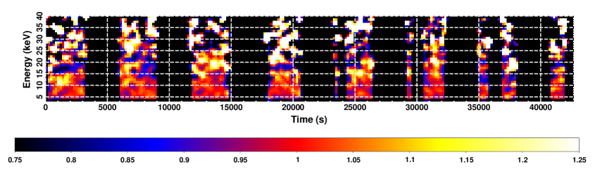
Figure 7.— Time-energy image (normalized to the time-averaged $NuSTAR$ spectrum and light curve), using $NuSTAR$ events in the 3-40 keV energy range. The color scale marks in blue/black a deficit of counts (i.e. an absorption feature) with respect to the time-averaged $NuSTAR$ spectrum (whose level is at 1). The image at the highest energies is more noisy due to much lower number of counts per pixel.

A further spectral investigation was performed considering flare peaks simultaneously observed by $XMM$-$Newton$ and $NuSTAR$. This led to four flare peaks (marked with numbers 4, 5, 6 and 7). We extracted strictly simultaneous spectra (0.4-78 keV) and performed a new broad-band spectroscopy. We adopted the same models used to fit the time-averaged 0.4-78 spectrum (Table LABEL:tab:simflares). When required by the presence of negative residuals, we report also the fit results obtained with the inclusion of a cyclabs model, although in no case is the line significant. We note that similar results were obtained using a Gaussian line in absorption (gabs in xspec) instead of cyclabs, and a Comptonization continuum model (compTT) instead of a PLCUT model.

3.2.3 Not only flares: the lowest intensity state

To investigate the broad-band spectrum taken from the lowest intensity state where simultaneous $XMM$-$Newton$ and $NuSTAR$ were available, we accumulated a spectrum from the valleys just before and after flare n. 4. A meaningful spectroscopy could be performed in the energy band 0.8-30 keV. Also in this low luminosity state (L_X$\sim$3$\times$10³⁵ erg s^-1, 0.1-100 keV, see below), a fit with a single absorbed power-law revealed structured residuals, with a low energy excess and a roll-over at high energy (Fig. 8). A simple double-component model, with a power law plus a blackbody (equally absorbed), already provided a good fit ($\chi^{2}_{\nu}$/dof=0.939/267) to the emission (0.8-30 keV), resulting in an absorbing column density N_H=2$\times 10^{22}$ cm^-2, $\Gamma$=1.3, kT_BB=1.3 keV and a blackbody radius R_BB$\sim$150 m. In order to compare the spectral properties of the low state with other intensity states, we adopted both Model 1 and Model 2, fixing both Fe line properties and the power law cutoff to the time-averaged spectral shapes, since in the low intensity state these latter were unconstrained. The results are reported in Table LABEL:tab:low_spec, to be compared with Table LABEL:tab:simflares (flares) and Table LABEL:tab:av_spec (time-averaged spectrum).

Figure 8.— Broad-band spectrum of the lowest intensity state. Counts spectra are shown together with the residuals (in units of standard deviation) with respect to a simple absorbed power law, to clearly show the structures in the residuals.

Table 5Broad-band spectrum during the lowest intensity state (0.8–30 keV).

Parameter	Model 1	Model 2
NH ($10^{22}$ cm-2)	$1.52^{+0.37}_{-0.33}$	$0.84^{+0.93}_{-0.77}$
NHpcfabs ($10^{22}$ cm-2)	none	$2.1^{+2.2}_{-0.7}$
fpcfabs	none	$0.82^{+0.16}_{-0.52}$
kTBB (keV)	$1.43^{+0.19}_{-0.15}$	none
${\rm R_{BB}}$ (m)	$280\pm{70}$	none
$\Gamma$a	$0.78^{+0.18}_{-0.21}$	$0.98^{+0.09}_{-0.08}$
Ecut (keV)	$9.7$ fixed	$5.5$ fixed
Efold (keV)	$14.3$ fixed	$15.3$ fixed
Eline (keV)	$6.44$ fixed	$6.45$ fixed
$\sigma$line (keV)	$0$ fixed	$0$ fixed
Fluxline (ph cm-2 s-1)	3.2$\times 10^{-5}$ fixed	3.2$\times 10^{-5}$ fixed
EWlineb (eV)	$<120$	$<120$
Fluxc (erg cm-2 s-1)	(5.8$\pm{0.6}$) $\times$10-11	(6.1$\pm{0.2}$) $\times$10-11
Luminosityc (1035 erg s-1)	3.4$\pm{0.4}$	3.6$\pm{0.1}$
$\chi^{2}_{\nu}$/dof	0.911/267	0.911/267

3.2.4 Spin-phase resolved spectroscopy

A spin-phase resolved spectroscopy was performed on strictly simultaneous $XMM$-$Newton$ and $NuSTAR$ data. From the hardness ratios reported in Fig. 3 a spin-phase resolved spectral extraction driven by the source hardness would suggest different spectral extractions, depending on the energy bands adopted. So, we simply divided the pulse period into five equally spaced intervals, and extracted five broad-band (0.4-78 keV) spectra. Note that we tried also narrower or broader spin-phase intervals, but we found that five is the best compromise to map eventual spectral variability, given the available counts statistics.

The same models adopted before (Model 1 and Model 2) were applied to the five spectra resulting in the spectral parameters reported in Table LABEL:tab:spinphasespec and summarized in Fig. 9. The evolution of the intensity along the pulse profile is dominated by the variability of the power-law flux (2-10 keV), while the spectral variability seems to be mainly due to the power-law slope, which is the hardest in the first spin-phase interval ($\Delta\phi$=0.0-0.2), although the significant variability of the power law cutoff energy and of the blackbody parameters (in Model 1) along the spin phase did not allow us a straightforward interpretation.

When adopting Model 2, E_cut and E_fold parameters remained constant along the pulse profile. For this reason, we performed a second fit, fixing them to their mean value. We show in Fig. 10 the resulting confidence contour levels of the photon index and the additional absorbing column density partially covering the power law. The numbers indicate the five spin-phase-intervals. In these fits, the covering fraction in the five spectra was consistent with each other (within 90% uncertainty), in the range 0.52-0.67. Again, spin-phase interval $\phi$=0.0-0.2 showed a harder power law emission.

No significant negative residuals around 16-18 keV were found during the spin-phase resolved spectroscopy.

Table 6Broad-band (0.4-78 keV) spin-phase-resolved spectroscopy^a

Model 1 Parameters	$\Delta\phi$=0.0-0.2	0.2-0.4	0.4-0.6	0.6-0.8	0.8-1.0
NH ($10^{22}$ cm-2)	$0.91^{+0.20}_{-0.14}$	$1.0\pm{0.16}$	$1.01^{+0.13}_{-0.18}$	$1.04^{+0.16}_{-0.17}$	$1.20^{+0.23}_{-0.21}$
kTBB (keV)	$1.39^{+0.08}_{-0.10}$	$1.73^{+0.28}_{-0.12}$	$1.92^{+0.09}_{-0.16}$	$1.65^{+0.12}_{-0.10}$	$1.78^{+0.20}_{-0.09}$
${\rm R_{BB}}$ (m)	$630^{+60}_{-80}$	$490^{+75}_{-60}$	$400^{+50}_{-30}$	$430^{+60}_{-50}$	$430^{+70}_{-50}$
$\Gamma$	$-0.16^{+0.38}_{-0.57}$	$0.60^{+0.36}_{-0.19}$	$0.96^{+0.09}_{-0.21}$	$0.85^{+0.14}_{-0.17}$	$0.75^{+0.24}_{-0.24}$
Ecut (keV)	$7.1^{+0.8}_{-0.9}$	$9^{+7}_{-9}$	$21^{+2}_{-5}$	$13.0^{+1.7}_{-1.7}$	$10^{+6}_{-2}$
Efold (keV)	$9.5^{+2.4}_{-2.1}$	$16^{+8}_{-3}$	$12^{+6}_{-3}$	$15^{+3}_{-3}$	$21^{+20}_{-7}$
Pow Fluxb ($10^{-11}$ erg cm-2 s-1)	$3.6\pm{0.7}$	$4.4\pm{0.4}$	$2.62\pm{0.15}$	$2.51^{+0.15}_{-0.29}$	$2.9^{+0.3}_{-0.3}$
$\chi^{2}_{\nu}$/dof	0.988/782	1.014/943	1.011/749	1.043/655	0.997/752
Model 2 Parameters	$\Delta\phi$=0.0-0.2	0.2-0.4	0.4-0.6	0.6-0.8	0.8-1.0
NH ($10^{22}$ cm-2)	$0.9^{+0.41}_{-0.15}$	$1.38\pm{0.18}$	$1.26^{+0.14}_{-0.15}$	$1.45^{+0.18}_{-0.21}$	$1.50^{+0.22}_{-0.20}$
NHpcfabs ($10^{22}$ cm-2)	$3.2^{+1.0}_{-0.19}$	$7.6^{+2.7}_{-2.6}$	$7.9^{+2.2}_{-2.1}$	$8.6^{+2.7}_{-3.0}$	$6.8^{+2.7}_{-2.1}$
fpcfabs	$0.77^{+0.01}_{-0.11}$	$0.54^{+0.07}_{-0.09}$	$0.57^{+0.07}_{-0.08}$	$0.56^{+0.09}_{-0.17}$	$0.58^{+0.07}_{-0.08}$
$\Gamma$	$1.00^{+0.09}_{-0.04}$	$1.13^{+0.17}_{-0.18}$	$1.22^{+0.15}_{-0.15}$	$1.35^{+0.21}_{-0.37}$	$1.18^{+0.17}_{-0.15}$
Ecut (keV)	$6.5^{+0.7}_{-0.6}$	$6.4^{+1.1}_{-0.9}$	$6.5^{+0.8}_{-0.8}$	$6.4^{+1.6}_{-6.4}$	$6.4^{+0.89}_{-0.72}$
Efold (keV)	$19.8^{+2.6}_{-1.2}$	$18^{+5}_{-3}$	$17^{+4}_{-3}$	$20^{+7}_{-6}$	$18^{+6}_{-3}$
Pow Fluxb ($10^{-11}$ erg cm-2 s-1)	$7.0^{+0.16}_{-0.13}$	$9.8^{+0.5}_{-0.4}$	$7.5^{+0.38}_{-0.32}$	$6.1^{+0.39}_{-0.33}$	$7.3^{+0.4}_{-0.3}$
$\chi^{2}_{\nu}$/dof	0.984/782	1.027/943	1.013/749	1.046/655	0.987/752

Figure 9.— Results of the spin-phase-resolved spectroscopy of $XMM$-$Newton$ and $NuSTAR$ simultaneous observations (the spectral parameters and their physical units are the same reported in Table LABEL:tab:spinphasespec). Left panel shows the spectral paramenters with Model 1, while Right panel the results with Model 2. The top panels display the pulse profiles in two energy ranges for comparison: 0.4-12 keV (solid line) and 12-78 keV (dashed line).

Figure 10.— Confidence contour levels (68%, 90% and 99%) for the power law photon index and the additional absorbing column density partially covering the X-ray emission along the spin phase. The resulting covering fractions in the five spectra are consistent with each other (within 90% uncertainty), and their values are in the range 0.52-0.67. Numbers mark the five spin-phase-intervals. See Sect. 3.2.4 for details.

3.2.5 Hardness-ratio-selected spectroscopy

We investigated the spectral variability along the observation plotting different hardness ratios versus time. Whatever choice of hardness ratio (in both $XMM$-$Newton$ and $NuSTAR$ data), some level of scatter around a mean value was always present, but with no clear trend suggesting a specific and meaningful hardness-ratio-selected spectroscopy. The only exception was in case of the hardness ratio of 4-12 keV to 1-4 keV count rates (Fig. 11): a hard peak lasting $\sim$500 s in the hardness ratio was found after 10⁴ s from the start of the $XMM$-$Newton$ observation. We extracted an $XMM$-$Newton$ spectrum from this time interval (“hard dip”, hereafter), as it was not simultaneously covered by $NuSTAR$. Meaningful spectroscopy was possible in the energy range 1-10 keV. A single absorbed power law model resulted in an absorbing column density N_H=(3.2$\pm{0.6}$)$\times 10^{22}$ cm^-2, $\Gamma$=0.8${}^{+0.16}_{-0.15}$, and a flux corrected for the absorption F=3.9$\times 10^{-11}$ erg cm^-2 s^-1 (1–10 keV). Adopting more complicated models (like Model 1 and Model 2) is meaningless, since several spectral parameters are unconstrained.

Figure 11.— $XMM$-$Newton$ EPIC pn light curves in two energy ranges (Soft = 1-4 keV; Hard = 4-12 keV), together with their hardness ratio (H/S) in the third panel. Bin time is 187 s. The only short time interval where a hardness ratio variability is evident, has been marked in the bottom panel as “hard dip” and considered for further spectral analysis (Sect. 3.2.5). The horizontal line is the fit to the hardness ratio with a constant model.

4. Discussion

We have reported on the joint observation of the SFXT IGR J11215–5952 with $XMM$-$Newton$ and $NuSTAR$, performed during the expected times of the 2016 February outburst. These observations caught the source in outburst at its peak (L_X$\sim$10³⁶ erg s^-1), as confirmed by the monitoring of the light curve performed with $Swift$/XRT (Fig. 1).

The X–ray light curve showed several bright flares with a dynamic range of one order of magnitude during the outburst. The X–ray pulsar did not show evidence for spin period derivatives with respect to previous observations performed a decade ago (Swank et al., 2007; Sidoli et al., 2007). The rotational modulation is detected for the first time also at hard energies with $NuSTAR$, with an energy-dependent spin profile, evolving from an asymmetric main peak dominating at softer energies, to a single more symmetric peak at hard energies above $\sim$12 keV.

The source spectrum could be investigated for the first time simultaneously from 0.4 to 78 keV. It showed a complex structure that could not be described by a single absorbed power law, with a soft excess together with a cutoff at high energies. Different spectral models were investigated, obtaining a good fit with a phenomenological double-component continuum composed by a blackbody together with a PLCUT model (Model 1). This description is typically adopted in the X–ray spectroscopy of highly magnetized accreting pulsars (Coburn et al., 2002), where the power law is due to Comptonization in the accretion column and the blackbody could have different origins (see below).

We also explored an alternative deconvolution of the spectrum (a single-component model composed by a PLCUT), where the structures in the residuals at softer energies were accounted for by a partially covering absorption model, instead of a blackbody. This second model (Model 2) resulted into an equivalently good description of the spectrum and it is worth reporting, since it is also adopted in the literature when investigating spectra from HMXB pulsars (e.g. Malacaria et al. 2016). A narrow emission line is present in the time-averaged spectrum at an energy of 6.44 keV (consistent with fluorescent emission from almost neutral iron) and a low equivalent width of 40 eV. During other spectral selections, the faint emission line is not clearly visible, although it is still consistent with being there with a similar flux. Fe lines with similar properties are normally found in the X-ray spectra of HMXB pulsars and are interpreted as produced by fluorescent emission in the wind of the supergiant donor illuminated by the X–ray pulsar (Giménez-García et al., 2015).

In both models, the PLCUT continuum resulted in a flat slope (with a harder photon index in Model 1 than in Model 2), and in energies of the cutoff that are in agreement with what found in other X–ray pulsars spectra (Coburn et al., 2002). The blackbody emission in Model 1 resulted in a hot temperature of 1.6 keV from a small area of 460 meters (at a distance of 7 kpc). Such soft excesses have been discovered in different types of accreting pulsars (see La Palombara & Mereghetti 2006 for a review), with two different properties: hot temperatures (1-2 keV) with small emission radii of a few hundred meters, versus colder blackbodies (0.1-0.5 keV) with a much larger emitting radius (R_BB$\sim$100 km). The blackbody component in IGR J11215–5952 is consistent with what found in low luminosity accreting pulsars (L_X$\sim$10³⁴-10³⁶ erg s^-1), where the hot and small blackbody is thought to be emitted from the polar cap of the accreting pulsar (La Palombara et al., 2012).

Comparing the X-ray flare spectra, we rely on the broad-band $XMM$-$Newton$ and $NuSTAR$ simultaneous spectroscopy (Table LABEL:tab:simflares). In this case, only Model 1 provided evidence of variability in the spectral parameters with flux, where harder slopes are found during brighter flare peaks (the faintest flare n.7 shows a significantly steeper power law), again in agreement with what usually found in HMXB pulsars (e.g., Walter et al. 2015; Martínez-Núñez et al. 2017 for reviews). On the other hand, a similar trend in not present when using Model 2, where all parameters are consistent with being constant within the 90% uncertainties. When compared with the spectrum extracted from the low intensity region of the light curve, only Model 1 resulted in softer spectral parameters when the source is fainter (as usually observed in HMXB pulsars and SFXTs).

The absorption column density resulting from both models is always in excess of the total Galactic (8$\times$10²¹ cm^-2, Dickey & Lockman 1990), consistent with local absorbing material, explained by the supergiant outflowing wind. In Model 2, the power law continuum is partially covered (around 50%) by an additional local absorbing column density. The physical meaning of a partial covering absorption might be ascribed to the clumpiness of the circumsource material, where the partial absorbers could be due to blobs in the donor wind. A denser wind clump passing in front of the X-ray source could also explain the hard dip lasting about 500 s caught during the uninterrupted $XMM$-$Newton$ observation.

During the spectroscopy of single flare peaks, we found a hint of an absorption feature at 17 keV that, if described with a cyclotron absorption model, resulted in a line significance of 2.63 $\sigma$ (including trials) derived by means of Monte Carlo simulations. Given the low significance, the presence of this line cannot be claimed and needs further confirmation. However, we note that if real, it is variable, since it is present neither in the time-averaged spectrum nor in the spin-phase selected spectroscopy. This might resemble the behavior in another SFXT, IGRJ17544-2619, where a temporary cyclotron line was found. The cyclotron line at 16.8 keV discovered in $NuSTAR$ data by Bhalerao et al. (2015), was not confirmed by Bozzo et al. (2016) during another $NuSTAR$ observation at a similar source flux.

4.1. The SFXT scenario

After ten years since SFXTs discovery, a huge progress has been made in understanding their behaviour.

At first, it was proposed that Bondi-Hoyle direct accretion from dense clumps in the supergiant wind could explain the sporadic flaring activity in SFXTs (in’t Zand, 2005). A comparison of the clump properties implied by the SFXT X–ray light curves with what predicted by the theory of line-driven hot stellar winds indicate that direct Bondi-Hoyle accretion from clumpy winds cannot reproduce the X-ray data (see Martínez-Núñez et al. 2017 and references therein for a comprehensive review). One of the difficulties of the clumpy wind scenario is that the accreted mass derived from the SFXT X–ray flares (10¹⁹-10²² g) is typically larger than what expected from a single clump in stellar winds ($\sim$10¹⁸ g). The IGR J11215–5952 flare peak luminosity implies an accreted mass of $\sim$10¹⁹ g onto the NS, confirming once more this discrepancy. Note that this mass should be considered as a lower limit to the clump mass, since a wind blob, if it is larger than the accretion radius, might be only partially accreted by the pulsar.

Currently, two physical mechanisms might explain the SFXT flares in a 187 s pulsar like IGR J11215–5952: either a centrifugal barrier (Grebenev & Sunyaev, 2007; Bozzo et al., 2008)), or a quasi-spherical settling accretion regime (Shakura et al., 2012, 2014). In the first case, rescaling the Grebenev & Sunyaev (2007) equations to IGR J11215–5952 (spin period of 187 s and orbital period of 165 days) we derived a magnetic field of 1.2$\times$10¹³ G needed to have an operating centrifugal barrier (although we note that the equations reported by Grebenev & Sunyaev (2007) assume a circular orbit). If we adopt the average outburst X-ray luminosity of 10³⁶ erg s^-1 instead of the wind parameters in this scenario, we found an even higher estimate for the magnetic field of $\sim$5$\times$10¹³ G needed for the centrifugal barrier to operate. Note that also the source distance of 7 kpc is not accurate, but it should be considered as a lower limit (Lorenzo et al., 2014). In the second case, the settling accretion scenario sets in in slow pulsars (spin period $>$70 s) when the X–ray luminosity is below 4$\times$10³⁶ erg s^-1 (Shakura et al., 2012). Below this threshold the matter captured inside the Bondi radius is not able to efficiently cool down by Compton processes, so that it cannot penetrate the NS magnetosphere by means of Rayleigh-Taylor instabilities. Hot matter accumulates above the NS magnetosphere forming a quasi-static shell that cools down only by inefficient radiative cooling. Shakura et al. (2014) proposed that the bright SFXT flares are produced by the collapse onto the NS of this hot shell, triggered by reconnection events between the magnetic field carried by the accreting matter and the neutron star magnetosphere.

Quasi-periodic flaring activity that has often been observed to punctuate the SFXT outbursts (e.g. SAX J1818.6-1703, Boon et al. 2016), would be produced when the shell, after a collapse, is replenished by new wind capture, so the flares repeat on a regular timescale, as long as the mass accretion into the magnetosphere is allowed. The energy normally released in an SFXT bright flare ($\sim$10³⁹ erg) is in agreement with estimated mass of the hot shell (Shakura et al., 2014), that is also consistent with the accreted mass we have derived here from the luminosity of the flares in IGR J11215–5952 ($\sim$10¹⁹ g)

Our $XMM$-$Newton$ and $NuSTAR$ observations of IGR J11215–5952 allowed us also to observe, for the first time in this source, X-ray flares repeating every $\sim$2-2.5 ks, a property that in the settling accretion scenario is explained in a natural way. Note that the IGR J11215–5952 X–ray luminosity during outburst is fully compatible with the luminosity threshold predicted by Shakura et al. (2012) for the onset of the settling accretion. All these observational facts strongly favour an interpretation of the IGR J11215–5952 SFXT properties within the quasi-spherical settling accretion model.

Finally, we note that if the hint of a cyclotron line at 17 keV will be confirmed by future observations (implying a NS surface magnetic field of 2$\times$10¹² G), it will reinforce the interpretation of the SFXT behavior within the settling accretion scenario.

5. Conclusions

We have performed for the first time a temporal and spectral analysis of the SFXT pulsar IGR J11215–5952  simultaneously in the broad-band 0.4-78 keV. Indeed, the broadest X–ray energy band previously available for this source was the 5–50 keV range, thanks to INTEGRAL observations (Sidoli et al., 2006). The spin period (187.0 $\pm{0.4}$ s) did not show evidence for variability with respect to previous observations. Pulsations were detected for the first time above 12 keV, showing an energy dependent spin profile. The broad-band spectra was successfully deconvolved adopting a double-component model made of a power law with a high energy cutoff together with a hot blackbody, which we interpret as emission from the polar caps of the NS. Alternatively, a partial covering model replacing the blackbody component resulted into an equally good description of the data. The source light curve showed several bright flares spanning one order of magnitude in intensity, reaching 2$\times 10^{36}$ erg s^-1 at peak. The X–ray luminosity in outburst, together with the quasi-periodicity in the flaring activity caught during the uninterrupted $XMM$-$Newton$ observation, favour a quasi-spherical settling accretion model as the physical mechanism explaining the SFXT behavior, although alternative possibilities (e.g. centrifugal barrier) cannot be ruled out.

References

- Balucinska-Church & McCammon (1992) Balucinska-Church, M., & McCammon, D. 1992, ApJ, 400, 699
- Barrière et al. (2015) Barrière, N. M., Krivonos, R., Tomsick, J. A., et al. 2015, ApJ, 799, 123
- Bhalerao et al. (2015) Bhalerao, V., Romano, P., Tomsick, J., et al. 2015, MNRAS, 447, 2274
- Boon et al. (2016) Boon, C. M., Bird, A. J., Hill, A. B., et al. 2016, MNRAS, 456, 4111
- Bozzo et al. (2008) Bozzo, E., Falanga, M., & Stella, L. 2008, ApJ, 683, 1031
- Bozzo et al. (2015) Bozzo, E., Romano, P., Ducci, L., Bernardini, F., & Falanga, M. 2015, Advances in Space Research, 55, 1255
- Bozzo et al. (2016) Bozzo, E., Bhalerao, V., Pradhan, P., et al. 2016, A&A, 596, A16
- Coburn et al. (2002) Coburn, W., Heindl, W. A., Rothschild, R. E., et al. 2002, ApJ, 580, 394
- den Herder et al. (2001) den Herder, J. W., Brinkman, A. C., Kahn, S. M., et al. 2001, A&A, 365, L7
- Dickey & Lockman (1990) Dickey, J. M., & Lockman, F. J. 1990, ARA&A, 28, 215
- Evans et al. (2007) Evans, P. A., Beardmore, A. P., Page, K. L., et al. 2007, A&A, 469, 379
- Giménez-García et al. (2015) Giménez-García, A., Torrejón, J. M., Eikmann, W., et al. 2015, ArXiv e-prints, arXiv:1501.03636
- Grebenev & Sunyaev (2007) Grebenev, S. A., & Sunyaev, R. A. 2007, Astronomy Letters, 33, 149
- Harrison et al. (2013) Harrison, F. A., Craig, W. W., Christensen, F. E., et al. 2013, ApJ, 770, 103
- in’t Zand (2005) in’t Zand, J. J. M. 2005, A&A, 441, L1
- Jansen et al. (2001) Jansen, F., Lumb, D., Altieri, B., et al. 2001, A&A, 365, L1
- La Palombara & Mereghetti (2006) La Palombara, N., & Mereghetti, S. 2006, A&A, 455, 283
- La Palombara et al. (2012) La Palombara, N., Sidoli, L., Esposito, P., Tiengo, A., & Mereghetti, S. 2012, A&A, 539, A82
- Leahy et al. (1983) Leahy, D. A., Darbro, W., Elsner, R. F., et al. 1983, ApJ, 266, 160
- Lorenzo et al. (2014) Lorenzo, J., Negueruela, I., Castro, N., et al. 2014, A&A, 562, A18
- Lotti et al. (2016) Lotti, S., Natalucci, L., Mori, K., et al. 2016, ApJ, 822, 57
- Madsen et al. (2015) Madsen, K. K., Harrison, F. A., Markwardt, C. B., et al. 2015, ApJS, 220, 8
- Malacaria et al. (2016) Malacaria, C., Mihara, T., Santangelo, A., et al. 2016, A&A, 588, A100
- Martínez-Núñez et al. (2017) Martínez-Núñez, S., Kretschmar, P., Bozzo, E., et al. 2017, ArXiv e-prints, arXiv:1701.08618
- Negueruela et al. (2005) Negueruela, I., Smith, D. M., & Chaty, S. 2005, Astron. Tel., 470, 1
- Paizis & Sidoli (2014) Paizis, A., & Sidoli, L. 2014, MNRAS, 439, 3439
- Protassov et al. (2002) Protassov, R., van Dyk, D. A., Connors, A., Kashyap, V. L., & Siemiginowska, A. 2002, ApJ, 571, 545
- Romano et al. (2009) Romano, P., Sidoli, L., Cusumano, G., et al. 2009, ApJ, 696, 2068
- Sguera et al. (2005) Sguera, V., Barlow, E. J., Bird, A. J., et al. 2005, A&A, 444, 221
- Shakura et al. (2012) Shakura, N., Postnov, K., Kochetkova, A., & Hjalmarsdotter, L. 2012, MNRAS, 420, 216
- Shakura et al. (2014) Shakura, N., Postnov, K., Sidoli, L., & Paizis, A. 2014, MNRAS, 442, 2325
- Sidoli (2013) Sidoli, L. 2013, Proceedings of the 9th INTEGRAL workshop held in Paris, 2012, published online by Proceedings of Science (arXiv1301.7574), arXiv:1301.7574
- Sidoli et al. (2006) Sidoli, L., Paizis, A., & Mereghetti, S. 2006, A&A, 450, L9
- Sidoli et al. (2007) Sidoli, L., Romano, P., Mereghetti, S., et al. 2007, A&A, 476, 1307
- Sidoli et al. (2008) Sidoli, L., Romano, P., Mangano, V., et al. 2008, ApJ, 687, 1230
- Strüder et al. (2001) Strüder, L., Briel, U., Dennerl, K., et al. 2001, A&A, 365, L18
- Swank et al. (2007) Swank, J. H., Smith, D. M., & Markwardt, C. B. 2007, Astron. Tel., 999, 1
- Turner et al. (2001) Turner, M. J. L., Abbey, A., Arnaud, M., et al. 2001, A&A, 365, L27
- Walter et al. (2015) Walter, R., Lutovinov, A. A., Bozzo, E., & Tsygankov, S. S. 2015, A&A Rev., 23, 2
- Wilms et al. (2000) Wilms, J., Allen, A., & McCray, R. 2000, ApJ, 542, 914
- Winkler et al. (2011) Winkler, C., Diehl, R., Ubertini, P., & Wilms, J. 2011, Space Science Reviews, 161, 149
- Winkler et al. (2003) Winkler, C., Courvoisier, T., Di Cocco, G., et al. 2003, A&A, 411, L1