ZMP-HH/17-12
Hamburger Beiträge zur Mathematik Nr. 652
March 2017

Abstract
We give a detailed account of the so-called “universal construction” that aims to extend invariants of closed manifolds, possibly with additional structure, to topological field theories and show that it amounts to a generalization of the GNS construction. We apply this construction to an invariant defined in terms of the groupoid cardinality of groupoids of bundles to recover Dijkgraaf-Witten theories, including the vector spaces obtained as a linearization of spaces of principal bundles.

1 Introduction

The Gelfand-Naimark-Segal (GNS) construction associates to a $C^{\star}$ algebra $A$ and a state on $A$ a Hilbert space. Similar constructions work in a purely algebraic setting, and it has been known for a long time [Ker97, p.6][Ker03, p.32] that the construction of topological field theories from invariants of closed manifolds with links can be understood in this way. A Topological field theories is a symmetric monoidal functors from a category of cobordisms to a symmetric monoidal category, say vector spaces. The invariants of links in closed manifolds have various sources. One of them is the Kauffman bracket; the corresponding three-dimensional topological field theory has been constructed in [BHMV95]. Indeed, our general construction in section 2 of this note is inspired by [BHMV95] and many results in section 2 generalize results in [BHMV95].

Heuristically, the invariant for closed manifolds can be seen as the result of the evaluation of a path integral. In the simplest case of vanishing action, the path integral should count configurations. For gauge theories based on finite gauge groups, so-called Dijkgraaf-Witten theories [DW90] [FQ93], these configurations are finite groupoids; counting then means to determine the groupoid cardinality of this groupoid. In section 3, we explicitly deal with Dijkgraaf-Witten theories and exhibit a clear relation between groupoid cardinalities of bundles on three-manifolds with Wilson lines (or, more precisely, ribbon links) and linearizations of spaces of $G$-bundles on two-manifolds.

Our results admit several generalizations, including to theories in higher dimensions and to topological field theories with values in a monoidal category of modules over a commutative ring. Our results should also pave the way towards a more interesting and challenging generalization, a categorification of the present construction, leading to extended topological field theories.

2 The universal construction as a GNS construction

In this section, we present a general formulation of the GNS construction that is tailored to the construction of topological field theories from invariants of manifolds.

In a first step, we associate to a category $\mathcal{C}$ and an object $O\in\mathcal{C}$ two functors to the category $\text{vect}_{\mathbb{K}}$ of $\mathbb{K}$-vector spaces, where $\mathbb{K}$ is an arbitrary field,

 

and, dually,

$$\leavevmode\hbox to196.88pt{\vbox to37.58pt{\text{[drawing]}}}\;. {\mathcal{F}^{co}_{O}\colon\;\;\mathcal{C}^{\mathrm{opp}}} {\text{vect}_{\mathbb{K}}} \scriptstyle{\text{Hom}(\cdot,O)} \scriptstyle{\mathbb{K}[\cdot]} {\mathcal{F}^{co}_{O}\colon\;\;\mathcal{C}^{\mathrm{opp}}} {\text{vect}_{\mathbb{K}}} \scriptstyle{\text{Hom}(\cdot,O)} \scriptstyle{\mathbb{K}[\cdot]}$$

Here, $\mathbb{K}[\cdot]\colon\text{Set}\rightarrow\text{vect}_{\mathbb{K}}$ is the functor that assigns to a set the $\mathbb{K}$-vector space freely generated over the set. As an illustrative example inspired by [BHMV95], the reader might keep in mind the example where $\mathcal{C}$ is a category of cobordisms and $O=\emptyset$. Then $\text{End}_{\mathcal{C}}(O)$ are closed manifolds, possibly with additional structure, e.g. embedded links. In this situation, important examples of maps of sets $I\colon\text{End}_{\mathcal{C}}(O)\rightarrow\mathbb{K}$ are invariants of manifolds with embedded links. In general, we call a map of sets $I\colon\text{End}_{\mathcal{C}}(O)\rightarrow\mathbb{K}$ a state rooted in the object $O$.

A choice of a state $I$ rooted in $O$ defines for every object $c\in\mathcal{C}$ a bilinear pairing

$$\begin{array}[]{rrll}(\cdot,\cdot)_{c}\colon&\mathcal{F}_{O}(c)\otimes_{\mathbb{K}}\mathcal{F}^{co}_{O}(c)&\rightarrow&\mathbb{K}\\ &\delta_{f}\otimes\delta_{g}&\mapsto&I(g\circ f),\end{array}$$

where $\{\delta_{f}\mid f\in\text{Hom}(O,c)\}$ and $\{\delta_{g}\mid g\in\text{Hom}(c,O)\}$ are the canonical bases of the freely generated vector spaces $\mathcal{F}_{O}(c)$ and $\mathcal{F}^{co}_{O}(c)$, respectively. (If $\mathbb{K}$ is the field of complex numbers, a sesquilinear pairing can be constructed as well.) In general, these pairings are degenerate with a left radical $\text{lR}_{c}$ and right radical $\text{rR}_{c}$. We consider the quotients

$$\mathcal{F}_{O,I}(c):=\mathcal{F}_{O}(c)/\text{lR}_{c}\text{ and }\mathcal{F}^{co}_{O,I}(c):=\mathcal{F}^{co}_{O}(c)/\text{rR}_{c}\text{ for all }c\in\mathcal{C}$$

and denote the induced non-degenerate pairing between the vector spaces $\mathcal{F}_{O,I}(c)$ and $\mathcal{F}^{co}_{O,I}(c)$ by $\langle\cdot,\cdot\rangle_{c}$.

Lemma 1.

For any category $\mathcal{C}$ and any state $I\colon\text{End}_{\mathcal{C}}(O)\rightarrow\mathbb{K}$, we obtain well-defined functors $\mathcal{F}_{O,I}:\mathcal{C}\to\text{vect}_{\mathbb{K}}$ and $\mathcal{F}^{co}_{O,I}:\mathcal{C}^{\mathrm{opp}}\to\text{vect}_{\mathbb{K}}$.

Proof.

It remains to be shown that $\mathcal{F}_{O,I}$ and $\mathcal{F}^{co}_{O,I}$ are well-defined on morphisms. We present the proof for $\mathcal{F}_{O,I}$. It is enough to show that for all morphisms $h\in\text{Hom}_{\mathcal{C}}(c,c^{\prime})$ the image of the radical $\text{lR}_{c}\subset\mathcal{F}_{O}(c)$ under $\mathcal{F}_{O}[h]$ is contained in $\text{lR}_{c^{\prime}}\subset\mathcal{F}_{O}(c^{\prime})$. For $r=\sum_{i}a_{i}\delta_{f_{i}}\in\text{lR}_{c}$ and all $g\in\text{Hom}(c^{\prime},O)$, we find

$$(\mathcal{F}_{O}[h](r),\delta_{g})_{c^{\prime}} =\sum_{i}a_{i}I(g\circ(h\circ f_{i}))=\sum_{i}a_{i}(\delta_{f_{i}},\mathcal{F}^{co}_{O}[h](\delta_{g}))_{c}=(r,\mathcal{F}^{co}_{O}[h](\delta_{g}))_{c}=0\;.$$

∎

Definition 2.

We call the functors $\mathcal{F}_{O,I}$ and $\mathcal{F}^{co}_{O,I}$ a pair of GNS functors for the category $\mathcal{C}$ and the state $I:\mathrm{End}(O)\to\mathbb{K}$.

Remarks 3.

1. Exchanging $\mathcal{C}$ and its opposed category $\mathcal{C}^{op}$ exchanges the GNS functors $\mathcal{F}_{O,I}$ and $\mathcal{F}^{co}_{O,I}$. For this reason, it usually suffices to prove statements for the GNS functor $\mathcal{F}_{O,I}$.

2. A $\dagger$-structure on a category $\mathcal{C}$ is a involutive functor $\dagger:\mathcal{C}\rightarrow\mathcal{C}^{op}$ which is the identity on objects. A state $I\colon\text{End}_{\mathcal{C}}(O)\rightarrow\mathbb{K}$ is compatible with a $\dagger$-structure on $\mathcal{C}$, if $I(f^{\dagger})=I(f)$ for all $f\in\text{End}_{\mathcal{C}}(O)$. (In the case of the field of complex numbers, $\mathbb{K}=\mathbb{C}$, a sesquilinear variant of the condition, $I(f^{\dagger})=I(f)^{*}$, can be considered as well.)

   For a category with $\dagger$-structure and a compatible state $I$, we define for all $c\in\mathcal{C}$ a pairing by

   $$\begin{array}[]{rlll}(\cdot,\cdot)_{c,\dagger}\colon&\mathcal{F}_{O}(c)\otimes_{\mathbb{K}}\mathcal{F}_{O}(c)&\rightarrow&\mathbb{K}\\ &\delta_{f}\otimes\delta_{g}&\mapsto&I(g^{\dagger}\circ f)\;.\end{array}$$

   We then have $\mathcal{F}_{O,I}(c)=\mathcal{F}_{O}(c)/\text{lR}((\cdot,\cdot)_{c,\dagger})$ and $\mathcal{F}^{co}_{O,I}=\mathcal{F}_{O,I}\circ\dagger$.

Examples 4.

1. A $C^{\star}$-algebra $A$ can be seen as a one object $\mathbb{C}$-linear category $\bullet//A$ together with a $\dagger$-structure ${}^{\star}\colon\bullet//A\rightarrow(\bullet//A)^{op}$. A classical state $\tau\colon A=\mathrm{End}(\bullet)\rightarrow\mathbb{K}$ on $A$ is a state rooted in $\bullet$; it leads to a vector space $\mathcal{F}_{\bullet,\tau}(\bullet)$ endowed with a scalar product $\langle\cdot,\cdot\rangle_{\bullet}$. (In general $\mathcal{F}_{\bullet,\tau}(\bullet)$ is not a Hilbert space; by taking its completion, one obtains a Hilbert space together with an action of $A$. This is the the classical Gelfand-Naimark-Segal (GNS) construction.)

   The generalization of this example to $C^{\star}$-categories is straightforward, see [GLR85].

2. Following [BHMV95], consider a category whose objects are closed oriented two dimensional manifolds with $p_{1}$-structure and an even number of embedded arcs and where the morphisms are cobordisms with $p_{1}$-structure and ribbon links matching the arcs on the boundary.

   Then a state $\langle\;\;\rangle_{p}$ rooted in $\emptyset$ can be obtained from the Kauffman bracket and a primitive $2p$-th root of unity. In this context, the role of the GNS functors is to provide vector spaces assigned to codimension-one manifolds. The main theorem of [BHMV95] can be formulated using the language of this note as: The GNS functor corresponding to $\langle\;\;\rangle_{p}$ is symmetric monoidal for $p\geq 3$.

3. Section 3 contains a discussion of three-dimensional topological field theories in terms of GNS functors.

Inspired by the second example, we now assume that the category $\mathcal{C}$ has the structure of a monoidal category $(\mathcal{C},\otimes_{\mathcal{C}},\mathbb{I},a,r,l)$. Here, $\mathbb{I}$ is the monoidal unit, $a$ the associator and $r$ and $l$ are unit constraints. In this case, the monoidal unit $O=\mathbb{I}$ is a natural choice. Then $\text{End}_{\mathcal{C}}(\mathbb{I})$ has the additional structure of a unitary monoid.

Proposition 5.

There is a linear isomorphism $\varphi_{0}\colon\mathcal{F}_{\mathbb{I},I}(\mathbb{I})\rightarrow\mathbb{K}$ sending $\delta_{\text{id}_{\mathbb{I}}}$ to $1\in\mathbb{K}$, if and only if the state $I\colon\text{End}_{\mathcal{C}}(\mathbb{I})\rightarrow I$ is a morphism of unitary monoids.

Proof.

The multiplicativity of $I$ implies for all $f,g\in\text{End}_{\mathcal{C}}(\mathbb{I})$ with $I(g)\neq 0$ the relation

$$[\delta_{f}]=\frac{I(f)}{I(g)}[\delta_{g}]\in\mathcal{F}_{\mathbb{I},I}(\mathbb{I}),$$

where we denote by $[\cdot]$ the equivalence classes in $\mathcal{F}_{\mathbb{I},I}(\mathbb{I})$. $\mathcal{F}_{\mathbb{I},I}(\mathbb{I})$ is not zero dimensional, since $I(\text{id}_{\mathbb{I}})=1$. We leave the other direction to the reader. ∎

We will from now on assume that the state $I\colon\text{End}_{\mathcal{C}}(\mathbb{I})\rightarrow I$ is a morphism of unitary monoids. (This assumption typical does not hold for GNS states in quantum mechanics.) In general, the GNS functors are not necessarily monoidal; rather a weaker statement holds true:

Theorem 6.

Let $(\mathcal{C},\otimes_{\mathcal{C}},\mathbb{I},a,r,l)$ be monoidal category and $I\colon\text{End}_{\mathcal{C}}(\mathbb{I})\rightarrow\mathbb{K}$ a morphism of unitary monoids.

1. The natural transformation $\varphi_{2}\colon\mathcal{F}_{\mathbb{I},I}(\cdot)\otimes_{\mathbb{K}}\mathcal{F}_{\mathbb{I},I}(\cdot)\Rightarrow\mathcal{F}_{\mathbb{I},I}(\cdot\otimes_{\mathcal{C}}\cdot)$ defined for $c,c^{\prime}\in\mathcal{C}$ by

   $$\begin{array}[]{rlll}\varphi_{2,c,c^{\prime}}\colon&\mathcal{F}_{\mathbb{I},I}(c)\otimes_{\mathbb{K}}\mathcal{F}_{\mathbb{I},I}(c^{\prime})&\rightarrow&\mathcal{F}_{\mathbb{I},I}(c\otimes_{\mathcal{C}}c^{\prime})\\ &\delta_{f}\otimes\delta_{g}&\mapsto&\delta_{(f\otimes g)\circ r^{-1}}\end{array}$$

   is well-defined. The morphism $\varphi_{0}$ from proposition 5 and the natural transformation $\varphi_{2}$ endow the GNS functor $\mathcal{F}_{\mathbb{I},I}$ with the structure of a lax monoidal functor.
   

2. The natural transformation $\varphi_{2}$ is injective. Furthermore, it is an isomorphism, if and only if there exist for all pairs of objects $c,c^{\prime}\in\mathcal{C}$ and any morphism $f\in\text{Hom}(\mathbb{I},c\otimes_{\mathcal{C}}c^{\prime})$ a finite collection of morphisms $f_{c,i}\in\text{Hom}(\mathbb{I},c)$, $f_{c^{\prime},i}\in\text{Hom}(\mathbb{I},c^{\prime})$ and scalars $a_{i}\in\mathbb{K}$, such that

   $$I(g\circ f)=\sum_{i}a_{i}I(g\circ(f_{i,c}\otimes_{\mathcal{C}}f_{i,c^{\prime}}))$$ (1)

   for all $g\in\text{Hom}(c\otimes_{\mathcal{C}}c^{\prime},\mathbb{I})$.

In the definition of $\varphi_{2}$, we might have alternatively used $l^{-1}$ instead of $r^{-1}$; both morphisms however agree on the monoidal unit $\mathbb{I}$.

Proof.

1. We show that the natural transformation $\varphi_{2}$ is well-defined. Consider an arbitrary element $r=\sum_{i}a_{i}\delta_{f_{i}}\in\text{lR}_{c}$ with $f_{i}\in\text{Hom}(\mathbb{I},c)$. For all $g\in\text{Hom}(\mathbb{I},c^{\prime})$ and $h\in\text{Hom}(c\otimes_{\mathcal{C}}c^{\prime},\mathbb{I})$ we can calculate

   $$(\varphi_{2,X,Y}(r\otimes\delta_{g}),\delta_{h})_{c\otimes_{\mathcal{C}}c^{\prime}} =\sum a_{i}I(h\circ(f_{i}\otimes g)\circ r^{-1})=\sum a_{i}I(h\circ(\text{id}_{X}\otimes g)\circ(f_{i}\otimes\text{id}_{Y})\circ r^{-1})$$

   $$=\sum a_{i}I(h\circ(\text{id}_{X}\otimes g)\circ r^{-1}\circ f_{i})=(r,\delta_{h\circ(\text{id}_{X}\otimes g)\circ r^{-1}})_{c}=0\;.$$

   We can use the same argument for $r^{\prime}\in\text{lR}_{c^{\prime}}$. Using linearity this proves that $\varphi_{2}$ is well-defined.
   It is straightforward using the definition of a monoidal category to verify that $\varphi_{0}$ and $\varphi_{2}$ endow $\mathcal{F}_{\mathbb{I},I}$ with the structure of a lax monoidal functor.
   

2. We define a non degenerate bilinear pairing $\langle\cdot,\cdot\rangle_{c,c^{\prime}}\colon(\mathcal{F}_{\mathbb{I},I}(c)\otimes\mathcal{F}_{\mathbb{I},I}(c^{\prime}))\otimes_{\mathbb{K}}(\mathcal{F}^{co}_{\mathbb{I},I}(c)\otimes_{\mathbb{K}}\mathcal{F}^{co}_{\mathbb{I},I}(c^{\prime}))\rightarrow\mathbb{K}$ by

   $$\langle a\otimes_{K}b,m\otimes_{K}n\rangle_{c,c^{\prime}}=\langle a,m\rangle_{c}\cdot\langle b,n\rangle_{c^{\prime}}\;\forall a\in\mathcal{F}_{\mathbb{I},I}(c),\;b\in\mathcal{F}_{\mathbb{I},I}(c^{\prime}),\;m\in\mathcal{F}^{co}_{\mathbb{I},I}(c)\text{ and }n\in\mathcal{F}^{co}_{\mathbb{I},I}(c^{\prime})\;,$$

   for all $c,c^{\prime}\in\mathcal{C}$.

   The natural transformation $\varphi_{2}$ and its dual analogue $\varphi_{2}^{co}\colon\mathcal{F}_{\mathbb{I},I}^{co}(\cdot)\otimes_{\mathbb{K}}\mathcal{F}_{\mathbb{I},I}^{co}(\cdot)\Rightarrow\mathcal{F}_{\mathbb{I},I}^{co}(\cdot\otimes_{\mathcal{C}}\cdot)$ define a map

   $$\phi_{c,c^{\prime}}:(\mathcal{F}_{\mathbb{I},I}(c)\otimes_{\mathbb{K}}\mathcal{F}_{\mathbb{I},I}(c^{\prime}))\otimes_{\mathbb{K}}(\mathcal{F}^{co}_{\mathbb{I},I}(c)\otimes\mathcal{F}^{co}_{\mathbb{I},I}(c^{\prime}))\rightarrow\mathcal{F}_{\mathbb{I},I}(c\otimes_{\mathcal{C}}c^{\prime})\otimes_{\mathbb{K}}\mathcal{F}^{co}_{\mathbb{I},I}(c\otimes_{\mathcal{C}}c^{\prime})\;.$$

   This map preserves the non degenerate bilinear pairing, i.e.

   $$\langle a\otimes_{\mathbb{K}}b,m\otimes_{K}n\rangle_{c,c^{\prime}}=\langle\varphi_{2}(a\otimes_{\mathbb{K}}b),\varphi_{2}^{co}(m\otimes_{\mathbb{K}}n)\rangle_{c\otimes_{\mathcal{C}}c^{\prime}}\;.$$

   This implies that $\varphi_{2}$ is injective.

   Equation (1) implies

   $$[\delta_{f}]=\sum_{i}\varphi_{2}(a_{i}[\delta_{f_{ic}}]\otimes_{\mathbb{K}}[\delta_{f_{ic^{\prime}}}]),$$

   hence $\varphi_{2}$ is surjective if equation (1) holds. Obviously, equation (1) is true if $\varphi_{2}$ is surjective.

∎

The verification of the condition ensuring that $\varphi_{2}$ is an isomorphism can be quite complicated in concrete examples.

The following definition slightly generalizes the notion of a non-degenerate topological field theory [Tur10, III.3.1] and a cobordism generated functor [BHMV95, p.886]:

Definition 7.

Let $\mathcal{C}$ be a category and $O\in\mathcal{C}$. A functor $\mathcal{F}\colon\mathcal{C}\rightarrow\text{vect}_{\mathbb{K}}$ is $O$-exhausted, if $\mathcal{F}(c)=\text{span}_{\mathbb{K}}\{\text{Im}(\mathcal{F}(f))\mid f\in\text{Hom}(O,c)\}$ for all $c\in\mathcal{C}$.

GNS  functors based on an $O$-rooted state are obviously $O$-exhausted. Conversely, a pair of $O$-exhausted functors related by a non-degenerate bilinear pairing can be recognized as a pair of GNS  functors:

Proposition 8.

Let $(\mathcal{C},\otimes_{\mathcal{C}},\mathbb{I},a,r,l)$ be a monoidal category and $I\colon\text{End}_{\mathcal{C}}(\mathbb{I})\rightarrow\mathbb{K}$ a morphism of unitary monoids. Let $F\colon\mathcal{C}\rightarrow\text{vect}_{\mathbb{K}}$ and $F^{co}\colon\mathcal{C}^{op}\rightarrow\text{vect}_{\mathbb{K}}$ be a pair of $\mathbb{I}$-exhausted functors $F\colon\mathcal{C}\rightarrow\text{vect}_{\mathbb{K}}$ and $F^{co}\colon\mathcal{C}^{op}\rightarrow\text{vect}_{\mathbb{K}}$, which are related by non-degenerate bilinear pairings

$$\widetilde{\langle\cdot,\cdot\rangle}_{c}\colon F(c)\otimes F^{co}(c)\rightarrow\mathbb{K}$$

for all $c\in\mathcal{C}$. Suppose furthermore that there are isomorphisms

$$\varphi\colon\mathbb{K}\rightarrow F(\mathbb{I})\quad\text{ and }\quad\varphi^{co}\colon\mathbb{K}\rightarrow F^{co}(\mathbb{I})$$

compatible with the morphism $I$ in the sense that for all $c\in\mathcal{C}$ and all $f\in\text{Hom}(\mathbb{I},c)$ and $g\in\text{Hom}(c,\mathbb{I})$, we have

$$I(g\circ f)=\widetilde{\langle F(f)[\varphi(1)],F^{co}(g)[\varphi^{co}(1)]\rangle}_{c}\,\,.$$

1. Then there are natural isomorphisms $\alpha\colon\mathcal{F}_{\mathbb{I},I}\Rightarrow F$ and $\alpha^{co}\colon\mathcal{F}_{\mathbb{I},I}^{co}\Rightarrow F^{co}$ to the GNS functors for the state $I$.

2. These natural transformations are monoidal, if all functors involved are monoidal, with the isomorphisms $\varphi$ and $\varphi^{co}$ as part of the monoidal data.

Proof.

We define a natural transformation $\alpha^{\prime}\colon\mathcal{F}_{\mathbb{I},I}\Rightarrow F$ by $\alpha[\delta_{f}]=F(f)[\varphi(1)]$ and $\alpha_{co}^{\prime}$ in an analogous way. These maps are surjective and compatible with the bilinear pairing $(\cdot,\cdot)_{c}$ constructed from $I$. For this reason we get induced natural transformations $\alpha\colon\mathcal{F}_{\mathbb{I},I}\Rightarrow F$ and $\alpha_{co}\colon\mathcal{F}_{\mathbb{I},I,co}\Rightarrow F_{co}$. It is straightforward to check that these are natural isomorphisms. Using the definition of a monoidal functor it is not hard to prove that, under the assumption stated in the proposition, these natural transformations are also monoidal. ∎

A topological field theory is a symmetric monoidal functor $Z:\text{cob}_{n,n-1}\to\text{vect}_{\mathbb{K}}$, where $\text{cob}_{n,n-1}$ is a symmetric monoidal category of cobordisms. To apply GNS functors to topological field theories, it is important to notice that the construction is compatible with braidings on monoidal categories:

Proposition 9.

Let $(\mathcal{C},\otimes_{\mathcal{C}},\mathbb{I},a,r,l,c)$ be a braided monoidal category with braiding $c$. If the GNS functor rooted in the monoidal unit is monoidal, then it is also braided.

Proof.

The naturality of the braiding implies that for all $U,V\in\mathcal{C}$ and all $f_{U}\in\text{Hom}(\mathbb{I},U)$ and $f_{W}\in\text{Hom}(\mathbb{I},W)$ the diagram

commutes. The triangle commutes, since the braiding is compatible with the right unit constraint. [JS93, Proposition 1]. With this in mind, it is straightforward to check that the GNS  functor $\mathcal{F}_{\mathbb{I},I}$ is braided. ∎

Remarks 10.

1. The characterization of GNS  functors on (braided) monoidal categories implies that an $n$-dimensional topological field theory, i.e. a symmetric monoidal functor $Z:\text{cob}_{n,n-1}\to\text{vect}_{\mathbb{K}}$, can be reconstructed from its invariant on top-dimensional manifolds, if and only if $Z$ is $\emptyset$-exhausted. V. Turaev used this uniqueness to prove that every topological field theory of Reshetikhin-Turaev-type can be reconstructed [Tur10, Chapter III. Section 3+4 and Chapter IV. Lemma 2.1.3].

2. It is well-known that two-dimensional oriented topological field theories are classified by commutative Frobenius algebras (see for example [Koc04]). The topological field theory corresponding to the two-dimensional semi-simple Frobenius algebra $A=\text{span}(e_{1},e_{2})$ with multiplication $e_{i}\cdot e_{j}=\delta_{ij}e_{i}$ and co-unit $\epsilon(e_{1})=\epsilon(e_{2})=\lambda\in\mathbb{C}^{\star}$ is not $\emptyset$-exhausted: indeed, the image of any cobordism $\emptyset\stackrel{{\scriptstyle M}}{{\to}}\SS^{1}$ is contained in the one-dimensional subspace $\mathbb{C}(e_{1}+e_{2})$. (This situation changes if point defects are included, and one can then use the uniqueness result from proposition 8 to show that every two-dimensional topological field theory with point defects can be reconstructed using GNS functors.)

3 Three dimensional Dijkgraaf-Witten theories

We now turn to an application of GNS functors: the construction of three-dimensional oriented topological field theories. From now on, we will work over the field of complex numbers. We focus on a specific class of three-dimensional topological field theories, so-called Dijkgraaf-Witten theories. Dijkgraaf-Witten theories are gauge theories, based on a finite gauge group $G$. Our goal is to obtain them via GNS functors from quantities that are motivated by principles of gauge theory. To obtain GNS functors, we need:

• A monoidal category. This will be a monoidal category of three-dimensional oriented cobordisms. As usual for pure gauge theories, to have sufficiently many observables at our disposal, we will have to include Wilson lines.

• A state rooted in the monoidal unit, i.e. the empty set. This state should be thought of as the value of a “path integral” on a closed 3-manifold containing Wilson loops. For vanishing Lagrangian, such a value is given by counting configurations of gauge fields and thus by a groupoid cardinality of an essentially finite category of bundles.

We now set up these ingredients carefully. We will assume from now on that the gauge group $G$ is a finite abelian group. This assumption drastically reduces the technical complexity and still leads to theories that provide conceptual insight.

To describe the relevant symmetric monoidal category $\text{cob}_{G,3,2}$ including Wilson lines, we fix once and for all a standard torus $T^{2}$ embedded into $\mathbb{R}^{3}$ and a representative $\tau$ for every isomorphism class of principal $G$-bundles over $T^{2}$. An object $(\Sigma,(\mathfrak{a}_{1},\tau_{1}),\dots,(\mathfrak{a}_{n},\tau_{n}))$ of $\text{cob}_{G,3,2}$ consists of the following data:

• A smooth closed oriented two-dimensional manifold $\Sigma$,

• A finite number of ordered pairs of embedded arcs, described by an embedding $\mathfrak{a}_{i}\colon[-\tfrac{1}{10},\tfrac{1}{10}]\sqcup[-\tfrac{1}{10},\tfrac{1}{10}]\rightarrow\Sigma$. We require that the image of every $\mathfrak{a}_{i}$, i.e. the two arcs in a pair, is contained in the same connected component of $\Sigma$. Each such pair is labelled by a representative $\tau_{i}$ for a principal $G$-bundle over $T^{2}$.

Remarks 11.

1. For convenience, we label the first component of a pair by a $+$ sign and the second by a $-$ sign.

2. For an object $(\Sigma,(\mathfrak{a}_{1},\tau_{1}),\dots,(\mathfrak{a}_{n},\tau_{n}))\in\text{cob}_{G,3,2}$ we define $-(\Sigma,(\mathfrak{a}_{1},\tau_{1}),\dots,(\mathfrak{a}_{n},\tau_{n}))\in\text{cob}_{G,3,2}$ to be the object consisting of $\Sigma$ with reversed orientation and arcs constructed from the arcs $\mathfrak{a}_{i}$ by reversing the orientation of every arc and exchanging the order of every pair of arcs.

To define morphisms from $(\Sigma,(\mathfrak{a}_{1},\tau_{1}),\dots,(\mathfrak{a}_{n},\tau_{n}))$ to $(\Sigma^{\prime},(\mathfrak{a}^{\prime}_{1},\tau^{\prime}_{1}),\dots,(\mathfrak{a}^{\prime}_{m},\tau^{\prime}_{m}))$, consider smooth compact oriented three-dimensional manifolds $M$ with boundary $\partial M\cong-\Sigma\sqcup\Sigma^{\prime}$, together with an embedded ribbon link

$$l\colon\left(\bigsqcup_{i=1}^{n+m}[-\tfrac{1}{10},\tfrac{1}{10}]\times[0,1]\right)\sqcup\left(\bigsqcup_{j=1}^{k}[-\tfrac{1}{10},\tfrac{1}{10}]\times\SS^{1}\right)\rightarrow M$$

such that

• The intervals $[-\tfrac{1}{10},\tfrac{1}{10}]\times 0$ and $[-\tfrac{1}{10},\tfrac{1}{10}]\times 1$ are mapped to the negative and positive arcs in the boundary of $M$, respectively. The rest of the image of $l$ is contained in the interior of $M$; the intersection with the boundary is transversal.

• The ribbons induce the orientation opposite to the one given by the arcs.

• Every connected component of the image of $l$ is labelled with a principal $G$-bundle over the standard torus, such that they agree with the labels of the arcs on their boundary.

• The ribbon link respects the pair structure of the boundary arcs, in the sense that only the following ribbons are allowed between arcs:

  • A connected component of the link connecting the two arcs of a pair in the outgoing boundary or the two arcs of a pair in the ingoing boundary.

  • A pair of ribbon links connecting a pair of arcs in the ingoing boundary to a pair of arcs in the outgoing boundary.

Two such manifolds $(M,l)$ and $(M^{\prime},l^{\prime})$ are deemed to be equivalent if there exists an orientation preserving diffeomorphism relative boundaries $\varphi\colon M\rightarrow M^{\prime}$ mapping $l$ to $l^{\prime}$ that is compatible with all labels. These equivalence classes define the morphisms in $\text{cob}_{G,3,2}$.

Remarks 12.

1. Composition of morphisms is given by gluing along boundaries. Composition is only well-defined on equivalence classes of three-manifolds, since there is no canonical way of gluing smooth manifolds and ribbons, but all ways are diffeomorphic.

2. $\text{cob}_{G,3,2}$ is a symmetric monoidal category with the disjoint union of manifolds as tensor product and the empty set regarded as a two-dimensional manifold as monoidal unit.

As a second ingredient, we need a state rooted at $\emptyset$ which is also a morphism of unitary monoids $I\colon\text{End}_{\text{cob}_{G,3,2}}(\emptyset)\rightarrow\mathbb{K}$, i.e. a multiplicative invariant for all smooth closed oriented three-dimensional manifolds $M$ with embedded labelled ribbon links.

We consider the simplest possible gauge theories with vanishing action. (By including a a 3-cocycle in $Z^{3}(G,\mathbb{C}^{\times})$, one could incorporate a topological Lagrangian; we refrain from doing this in this short note.) Thus the state should be determined by counting gauge configurations, i.e. by the groupoid cardinality of an essentially finite groupoid of $G$-bundles over $M$. To set up our definition, we recall

Definition 13 (See e.g. definition 4 in [BHW10]).

Let $\mathcal{G}$ be an essentially finite groupoid and $\pi_{0}(\mathcal{G})$ the set of isomorphism classes of objects in $\mathcal{G}$. The groupoid cardinality of $\mathcal{G}$ is the positive rational number

$$|\mathcal{G}|=\sum_{g\in\pi_{0}(\mathcal{G})}\frac{1}{|\text{Aut}(g)|}\;,$$ (2)

where $|\text{Aut}(g)|$ is the cardinality of the automorphism group of a representative of $g$.

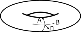
Figure 1: To orient $A$ and $B$ we chose an outwards pointing vector field $n$ on $T^{2}\subset\mathbb{R}^{3}$.

We define for manifolds $M$ without Wilson line defects

$$I_{DW,G}(M):=|\text{Bun}_{G}(M)|\;.$$ (3)

The case of three-manifolds with Wilson lines is slightly more involved. The label of a defect Wilson line should fix the behaviour of physical gauge fields “close” to the defect line.

To describe how this works in detail, we fix a meridian $A$ and a longitude $B$ on the standard torus in $\mathbb{R}^{3}$. We orient these circles as pictured in figure 1. An object of $\text{End}_{\text{cob}_{G,3,2}}(\emptyset)$ is represented by a closed manifold $M$, together with a labelled ribbon link $l\colon\sqcup_{i=1}^{n}\SS^{1}\times[-\tfrac{1}{10},\tfrac{1}{10}]\rightarrow M$. We define $M^{\prime}_{l}$ the three manifold with boundary obtained from $M$ with “small” open solid tori around the interior of every component of the ribbon link $l$ removed. The boundary of $M^{\prime}_{l}$ is thus diffeomorphic to a disjoint union of $n$ standard tori. We choose a diffeomorphism $\Phi\colon\sqcup_{i=1}^{n}T^{2}\rightarrow M^{\prime}_{l}$ such that the $B$-cycles of the standard tori are mapped onto boundary components of $l$ and the image of the $A$-cycles is contractable in the solid tori we removed before. This diffeomorphism is unique up to isotopy.

The labels of the components of $l$ determine, via the pullback along $\Phi^{-1}$, a principal $G$-bundle $P$ over $\partial M^{\prime}_{l}$. We denote by $\text{Bun}_{G,P}(M^{\prime}_{l})$ the groupoid of those principal $G$-bundles over the three-manifold $M^{\prime}_{l}$ which restrict to the isomorphism class of $P$ on $\partial M^{\prime}_{l}$.

Definition 14.

Let $G$ be a finite group. The Dijkgraaf-Witten state for gauge group $G$ on $\text{cob}_{G,3,2}$ rooted in $\emptyset$ is defined by its value on the three-manifold with Wilson lines $(M,l)$

$$I_{DW,G}(M,l):=|\text{Bun}_{G,P}(M^{\prime}_{l})|.$$ (4)

This extends the definition for manifolds without ribbon links in equation (3). One easily checks that this state is multiplicative. The rest of this paper is devoted to the computation of the GNS pair of functors corresponding to the Dijkgraaf-Witten state $I_{DW,G}$.

We first have to obtain a concrete understanding of the state $I_{DW,G}$. The well-known classification of principal $G$-bundles over a connected manifold $M$ is expressed in the following equivalence of groupoids

$$\text{Bun}_{G}(M)\cong\text{Hom}(H_{1}(M),G)//G\cong H^{1}(M,G)//G,$$ (5)

where $G$ acts on a group homomorphism $\varphi:H_{1}(M)\rightarrow G$ by conjugation. Since we assumed $G$ to be abelian, we can work with the first homology group, rather than the fundamental group. For an abelian group $G$, we thus identify isomorphism classes of principal $G$-bundles over $T^{2}$ with elements of $G\times G$. We agree that we identify the first component with the holonomy around the $A$-cycle and the second component with the holonomy around the $B$-cycle.

Example 15.

We determine $I_{DW,G}$ for an arbitrary $m$ component ribbon link $l$ in $\SS^{3}$, labelled by $(a_{1},b_{1}),\dots,(a_{m},b_{m})\in G\times G$. The first homology group of $(\SS^{3})^{\prime}_{l}$ is $\mathbb{Z}^{m}$. We chose $m$ cycles $A_{1},\dots,A_{m}$ going around one component of the ribbon link. We use the right hand rule to orient them. These cycles form a basis of $H_{1}((\SS^{3})^{\prime}_{l})$.

The two homotopic boundaries of every component of the link $l$ defines an element $B_{i}$ in $H_{1}((\SS^{3})^{\prime}_{l})$. We can express these elements in terms of the basis introduced above:

$$B_{i}=\sum_{j=1}^{m}m_{ij}A_{j}\>,$$ (6)

with coefficients $m_{ij}\in\mathbb{Z}$.

A group homomorphism $\varphi\colon H_{1}((\SS^{3})^{\prime}_{l})\rightarrow G$ and thus an isomorphism class of $G$-bundles is completely described by its value on the cycles $A_{i}$. Compatibility with the labels is equivalent to the following system of equations:

$$a_{i}=\varphi(A_{i})\;\; \forall i=1,\dots m$$ (7)

$$b_{i}=\sum_{j=1}^{m}m_{ij}\varphi(A_{j})\;\; \forall i=1,\dots m.$$ (8)

Inserting (7) into (8) leads to a system of $m$ linear conditions in $G$. The invariant corresponding to the link $l$ in $\SS^{3}$ is given by

$$I_{DW,G}(\SS^{3},l)=\begin{cases}\frac{1}{|G|}&\text{if condition \eqref{b_i=...} is satisfied}\\ 0&\text{otherwise}\end{cases}\>.$$ (9)

The computation of $I_{DW,G}(\SS^{3},l)$ can be involved in practice, since one has to express the boundary of every component of the link $l$ in terms of the generators of $H_{1}((\SS^{3})^{\prime}_{l})$. A more tractable approach is given by local relations which leave the Dijkgraaf-Witten state $I_{DW,G}$ invariant.

Proposition 16.

The invariant $I_{DW,G}$ for a labelled ribbon link $l$ in $\SS^{3}$ does not change under the following moves:

• 1. Move (figure 2(a)): Removing a complete right or left twist of a component labelled by $(a,b)\in G\times G$ and replacing the label $(a,b)$ by $(a,b-a)$ or $(a,b+a)$, respectively.

• 2. Move(figure 2(b)): Replace two parallel lines corresponding to the same connected component of a ribbon link $l$ in $\SS^{3}$ by a sum over elements of the form in figure 2(b).

• 3. Move (figure 2(c)): Removing an over-crossing followed by an under-crossing between a component $(k_{1},(b_{1},a_{1}))$ with a second not necessarily different component $(k_{2},(b_{2},a_{2}))$ and changing the labels to $(a_{1},b_{1}\pm a_{2})$ and $(a_{2},b_{2}\pm a_{1})$, where the sign depends on the relative orientation of the two components (compare figure 2(c)).

\begin{overpic}[scale={0.4}]{move1.pdf} \put(12.0,0.0){$(a,b)$} \put(28.0,0.0){$(a,b\!-\!a)$} \put(68.0,0.0){$(a,b)$} \put(84.0,0.0){$(a,b\!+\!a)$} \end{overpic}

(a) Graphical representation of move 1.

\begin{overpic}[width=284.52756pt,tics=10,scale={0.7}]{Move2.pdf} \put(2.0,21.0){$(a,b)$} \put(25.0,2.0){$(a,b)$} \put(50.0,15.0){\Huge{$\sum$}} \put(35.0,15.0){\Huge{$=$}} \put(47.0,9.0){$b_{1}\cdot b_{2}=b$ } \put(86.0,5.0){$(a,b_{1})$} \put(86.0,20.0){$(a,b_{2})$} \end{overpic}

(b) Graphical representation of move 2.

\begin{overpic}[width=284.52756pt,tics=10,scale={0.45}]{Move3.pdf} \put(-1.0,0.0){\tiny{$(a_{1},b_{1})$}} \put(8.0,0.0){\tiny$(a_{2},b_{2})$} \put(19.0,0.0){\tiny{$(a_{1},b_{1}\!+\!a_{2})$}} \put(33.0,0.0){\tiny{$(a_{2},b_{1}\!+\!a_{1})$}} \put(57.0,0.0){\tiny{$(a_{1},b_{1})$}} \put(66.0,0.0){\tiny$(a_{2},b_{2})$} \put(77.0,0.0){\tiny{$(a_{1},b_{1}\!-\!a_{2})$}} \put(91.0,0.0){\tiny{$(a_{2},b_{1}\!-\!a_{1})$}} \end{overpic}

(c) Graphical representation of move 3.

Figure 2: Graphical representation of proposition 16. The lines represent ribbons in positive blackboard framing.

Proof.

• Move 1 and 3: The first homology group of $(\SS^{3})^{\prime}_{l}$ does not change, if we apply move 1 or 3, but the cycles $B_{i}$ change. The change of the labels is chosen such that the resulting conditions are invariant.

• Move 2: We denote the link corresponding to a choice of $b_{1}$ and $b_{2}$ by $l_{b_{1},b_{2}}$. If the condition (8) is satisfied for $l_{b_{1},b_{2}}$ then it also holds for $l$. On the other hand there is exactly one $l_{b_{1},b_{2}}$ satisfying (8) for every $l$ satisfying (8).

∎

Remarks 17.

1. Move 3 can be used to interchange over- and under-crossings. This allows us to reduce every ribbon link in $\SS^{3}$ to a collection of simple unknotted links, providing an efficient algorithm for computing the value of the Dijkgraaf-Witten state $I_{DW,G}$ on links in $\SS^{3}$.

2. A result of [BHMV95] will allow us to generalize these relations to ribbon links in general three dimensional manifolds, cf.  corollary 23.

To explicitly describe the GNS functors $\mathcal{F}_{\emptyset,I_{DW,G}}$ for the Dijkgraaf-Witten state $I_{DW,G}$, we determine the vector space associated to a torus $T^{2}$ with the help of a Mayer-Vietoris argument.

Proposition 18.

Fix an untwisted ribbon link $k$ in the standard full torus such that the core of $k$ is homotopic to the $B$-cycle on the boundary. Each labelling of $k$ gives a morphism in $\text{Hom}(\emptyset,T^{2})$. The collection of these morphisms induces a basis of the vector space $\mathcal{F}_{\emptyset,I_{DW,G}}(T^{2})$. In particular the dimension of $\mathcal{F}_{\emptyset,I_{DW,G}}(T^{2})$ is $|G|\times|G|$.

Proof.

Suppose we are given connected cobordisms $(M,l)\in\text{Hom}(\emptyset,T^{2})$ and $(N,k)\in\text{Hom}(T^{2},\emptyset)$, together with group homomorphisms $\varphi_{M}\colon H_{1}(M^{\prime}_{l})\rightarrow G$ and $\varphi_{N}\colon H_{1}(N^{\prime}_{k})\rightarrow G$ which determine principal $G$-bundles on $M^{\prime}_{l}$ and $N^{\prime}_{l}$ compatible with the labels of $l$ and $k$.
By the Mayer-Vietoris sequence there is a pushout square

$$\leavevmode\hbox to144.51pt{\vbox to55.85pt{\text{[drawing]}}}\;. {H_{1}(T^{2})} {H_{1}((N)^{\prime}_{k})} {H_{1}((M)^{\prime}_{l})} {H_{1}((N\sqcup_{T^{2}}M)^{\prime}_{l\sqcup k})} {H_{1}(T^{2})} {H_{1}((N)^{\prime}_{k})} {H_{1}((M)^{\prime}_{l})} {H_{1}((N\sqcup_{T^{2}}M)^{\prime}_{l\sqcup k})}$$ (10)

The universal property of pushouts implies that there is a group homomorphism

$$\varphi_{N}\colon H_{1}((N\sqcup_{T^{2}}M)^{\prime}_{l\sqcup k})\rightarrow G$$

restricting to $\varphi_{M}$ and $\varphi_{N}$, if and only if $\varphi_{M}|_{T^{2}}=\varphi_{N}|_{T^{2}}$. Every group homomorphism corresponding to a bundle over $(N\sqcup_{T^{2}}M)^{\prime}_{l\sqcup k}$ compatible with all labels arises in this way. This implies that $v=\sum\alpha_{i}\delta_{(M_{i},l_{i})}\in\mathcal{F}_{\emptyset}(T^{2})$ and $v^{\prime}=\sum\alpha^{\prime}_{j}\delta_{(M^{\prime}_{j},k_{j})}\in\mathcal{F}_{\emptyset}(T^{2})$ are in the same equivalence class of $\mathcal{F}_{\emptyset,I_{DW,G}}(T^{2})$, if for all possible choices of principal $G$-bundles $P$ on $T^{2}$

$$\sum\alpha_{i}|\text{Bun}_{G,P\sqcup P(M_{i})}((M_{i})^{\prime}_{l_{i}})|=\sum\alpha^{\prime}_{j}|\text{Bun}_{G,P\sqcup P(M^{\prime}_{j})}((M^{\prime}_{j})^{\prime}_{k_{j}})|$$ (11)

holds. Here we denoted by $|\text{Bun}_{G,P\sqcup P(M_{i})}((M_{i})^{\prime}_{l_{i}})|$ the groupoid cardinality of the groupoid consisting of bundles over $(M_{i})^{\prime}_{l_{i}}$ such that these bundles restrict to the isomorphism class of the bundle defined by $P$ and the labels of links in $M_{i}$.
For a ribbon link $l$ as described in the proposition labelled by a principal $G$-bundle $\tau$ there is up isomorphism just one bundle on the boundary which can be extended to $(T^{2})_{l}^{\prime}$ compatible with the label. This bundle is $\tau$. This implies by (11) that such elements form a basis. ∎

To describe the functor on all objects of $\text{cob}_{G,3,2}$, we use a general result from Blanchet et al. [BHMV95], whose adaptation to $\text{cob}_{G,3,2}$ is straightforward. To state the result, we first need two definitions:

Definition 19 (p. 889 [BHMV95]).

We denote by $\mathbb{D}^{n}$ the $n$-dimensional closed unit ball.

A functor $Z\colon\text{cob}_{G,3,2}^{1}\rightarrow\text{vect}_{\mathbb{K}}$ with $Z(\emptyset)\cong\mathbb{K}$ is compatible with surgery, if:

• $Z(\SS^{3})\neq 0$.

• There is an $\eta\in\mathbb{K}$, such that $Z(\SS^{0}\times\mathbb{D}^{3})=\eta Z(\mathbb{D}^{1}\times\SS^{2})$.

• The element $Z(\mathbb{D}^{2}\times\SS^{1})$ lies in the sub vector space generated by ribbon links in the solid torus $-(\SS^{1}\times\mathbb{D}^{2})$.

Definition 20.

Let $M$ be a three-manifold with boundary $\partial M=\Sigma$ equipped with the structure of an object in $\text{cob}_{G,3,2}^{1}$. We denote by $\mathcal{L}(M,\Sigma)\subset\mathcal{F}_{\emptyset}(\Sigma)$ the vector space freely generated by the set of equivalence classes of ribbon links in $M$, which describe an element of $\text{Hom}_{\text{cob}_{G,3,2}}(\emptyset,\Sigma)$.

In [BHMV95], surgery for three-manifolds was used to show:

Proposition 21 (Proposition 1.9 of [BHMV95]).

If the $\emptyset$-exhausted lax functor from the universal construction $\mathcal{F}_{\emptyset,I}\colon\text{cob}_{G,3,2}^{1}\rightarrow\text{vect}_{\mathbb{K}}$ for a state $I$ is compatible with surgery, then for every $\Sigma\in\text{cob}_{G,3,2}$ and connected manifold $M$ with boundary $\Sigma$ the natural map $\pi\colon\mathcal{L}(M,\Sigma)\rightarrow\mathcal{F}_{\emptyset,I}(\Sigma)$ is surjective.
Furthermore, let $M^{\prime}$ be any 3-dimensional compact connected manifold with boundary $-\Sigma$, then the kernel of $\pi$ is the same as the left radical of the canonical pairing $(\cdot,\cdot)^{\prime}\colon\mathcal{L}(M,\Sigma)\otimes\mathcal{L}(M^{\prime},-\Sigma)\rightarrow\mathbb{K}$.

The reader should appreciate that the inclusion of co-dimension two defects, i.e. Wilson lines, is crucial for this result. To apply this result to the GNS functor $\mathcal{F}_{\emptyset,I_{DW,G}}$ for Dijkgraaf-Witten theories, we need to check its compatibility with surgery:

Lemma 22.

The GNS  functor $\mathcal{F}_{\emptyset,I_{DW,G}}$ is compatible with surgery.

Proof.

• Up to isomorphism, there is just one principal $G$-bundle over $\SS^{3}$, since $H_{1}(\SS^{3})$ is trivial. For this reason $I_{DW,G}(\SS^{3})=\tfrac{1}{|G|}\neq 0$.

• A Mayer-Vietoris argument similar to the argument in the proof of proposition 18 shows that the vector space $\mathcal{F}_{\emptyset,I_{DW,G}}(\SS^{2}\sqcup\SS^{2})$ is one dimensional. The structure of the groupoid cardinality is crucial for the argument to work.

  The elements in $\mathcal{F}_{\emptyset,I_{DW,G}}(\SS^{2}\sqcup\SS^{2})$ corresponding to the three-manifolds $\SS^{0}\times\mathbb{D}^{3}$ and $\mathbb{D}^{1}\times\SS^{2}$ are not zero, since there exists at least one principal $G$-bundle over every manifold.

• This requirement holds, since by proposition 18 $\mathcal{F}_{\emptyset,I_{DW,G}}(T^{2})$ is generated by ribbons in a full torus.

∎

We can now generalize proposition 16 to arbitrary manifolds.

Corollary 23.

The relations of proposition 16 hold in any closed oriented three-dimensional manifold.

Proof.

Using the compatibility with surgery we can relate the invariant for any ribbon link $l$ in a three dimensional manifold $M$ to a sum of invariants for links in $\SS^{3}$. We can apply to every term in the sum the relations of proposition 16. Reversing the surgery proves the relation for $l$ in $M$. ∎

We are now almost in a position to combine propositions 16 and 21 to obtain a concrete description of the GNS functor for the Dijkgraaf-Witten state $I_{DW,G}$. In this description, we will need a specific element which we construct first.

\begin{overpic}[width=284.52756pt,tics=10,scale={1}]{ExampleElement.pdf} \put(20.0,30.0){\scriptsize$(a_{1},\!b_{1})$} \put(70.0,30.0){\scriptsize$(a_{2},\!b_{2})$} \put(33.0,6.0){\scriptsize$(a,\!b)$} \put(60.0,6.0){\scriptsize$(a,\!b)$} \put(46.0,16.0){\scriptsize$(c_{1},\!a)$} \put(3.0,18.0){\scriptsize$k_{1}$} \put(94.0,19.0){\scriptsize$k_{2}$} \put(42.0,6.5){\scriptsize$l_{1}$} \put(50.0,10.5){\scriptsize$g_{1}$} \end{overpic}

Figure 3: An example for a manifold corresponding to the elements defined in remark 24 in the case of a manifold of genus $2$ with a pair of embedded arcs. For simplicity, only the core of the ribbon link is drawn.

Remark 24.

Let $(\Sigma_{g},(\mathfrak{a}_{1},\tau_{1}),\dots,(\mathfrak{a}_{n},\tau_{n}))\in\text{cob}_{G,3,2}$ be a connected surface of genus $g$ with $n$ pairs of embedded arcs. For each such surface, we fix a handle body $H_{g}$ bounding $\Sigma_{g}$, with the following additional structure (see also figure 3):

• A ribbon knot $k_{i}$ going around every hole of $H_{g}$, a ribbon knot $l_{j}$ connecting every pair of arcs on the boundary and an untwisted “small” ribbon $g_{j}$ going around $l_{j}$ oriented according to the right hand rule.

• The labels of the ribbon knots $l_{j}$ are determined by the labels of the arcs on the boundary $\Sigma_{g}$. We set the $B$-cycle holonomy of the small ribbons $g_{j}$ equal to the $A$-cycle holonomy of the corresponding ribbon $l_{j}$.

Any choice of the remaining labels $((a_{1},b_{1}),\dots,(a_{g},b_{g}),c_{1},\dots,c_{n})\in G^{2g+n}$ determines a non-zero element. We denote the corresponding element of the vector space $\mathcal{F}_{\emptyset,I_{DW,G}}((\Sigma_{g},...))$ by $\delta_{(a_{1},b_{1}),\dots,(a_{g},b_{g}),c_{1},\dots,c_{n}}$.

Theorem 25.

Let $G$ be a finite group, $\text{cob}_{G,3,2}$ the cobordism category with Wilson lines introduced at the beginning of this section and $I_{DW,G}$ be the Dijkgraaf-Witten state introduced in definition 14.

1. The GNS  functor $\mathcal{F}_{\emptyset,I_{DW,G}}\colon\text{cob}_{G,3,2}\rightarrow\text{vect}_{\mathbb{K}}$ based on the Dijkgraaf-Witten state is a symmetric monoidal functor and hence defines an oriented 3-2-dimensional topological field theory.

2. For any object $(\Sigma_{g},(\mathfrak{a}_{1},\tau_{1}),\dots,(\mathfrak{a}_{n},\tau_{n}))$ of $\text{cob}_{G,3,2}$, the family of vectors

   $$\left\{\delta_{(a_{1},b_{1}),\dots(a_{g},b_{g}),c_{1}\dots c_{n}}\mid((a_{1},b_{1}),\dots(a_{g},b_{g}),c_{1}\dots c_{n})\in G^{2g+n}\right\}$$

   form a basis of the vector space $\mathcal{F}_{\emptyset,I_{DW,G}}((\Sigma_{g},(\mathfrak{a}_{1},\tau_{1}),\dots,(\mathfrak{a}_{n},\tau_{n})))$.

Proof.

• We fix a handle body $H_{g}$ bounding $\Sigma_{g}$. We embed $H_{g}$ into $\SS^{3}$ and denote the closure of its complement by $M$. Proposition 21 implies

  $$\mathcal{F}_{\emptyset,I_{DW,G}}((\Sigma_{g},(\mathfrak{a}_{1},\tau_{1}),\dots,(\mathfrak{a}_{n},\tau_{n})))=\mathcal{L}(H_{g},(\Sigma_{g},(\mathfrak{a}_{1},\tau_{1}),\dots,(\mathfrak{a}_{n},\tau_{n})))/\text{lR}_{(\cdot,\cdot)^{\prime}}\;,$$

  with

  $$(\cdot,\cdot)^{\prime}\colon\mathcal{L}(H_{g},(\Sigma_{g},(\mathfrak{a}_{1},\tau_{1}),\dots,(\mathfrak{a}_{n},\tau_{n})))\otimes\mathcal{L}(M,-(\Sigma_{g},(\mathfrak{a}_{1},\tau_{1}),\dots,(\mathfrak{a}_{n},\tau_{n})))\rightarrow\mathbb{K}\>.$$

  \begin{overpic}[scale={1}]{RelationLabelRing.pdf} \put(7.0,10.0){$(a,b\!\pm\!c)$} \put(84.0,10.0){$(a,b)$} \put(36.0,25.0){\Huge{$=$}} \put(52.0,39.0){$(\pm c,a)$} \end{overpic}

  Figure 4: This relation allows us to change the labels of the ribbons connecting arcs to the value specified by the arcs after applying move 1, 2 and 3 inside $H_{g}$. To prove the relation apply move 3 on the right side and use that a contractable untwisted ribbon labelled by $(a,0)$ can be removed without changing the invariant.

  We can use the local relations developed in proposition 16 inside $H_{g}$, since the union of $H_{g}$ and $M$ is $\SS^{3}$. This changes the labels of the arcs on $\Sigma$. It is possible to compensate this by adding a ring around the ribbon using the relation in figure 4. These relations allow us to reduce every ribbon link in $H_{g}$ to a collection of knots going around every hole and ribbon links connecting the arcs on the boundary with small circles around them. From proposition 18 it follows that we can replace the collection of ribbon knots going around every hole by a sum over ribbon links with just one component going around every hole. This proves that the $\delta_{(a_{1},b_{1}),\dots(a_{g},b_{g}),c_{1}\dots c_{n}}$ generated $\mathcal{F}_{\emptyset,I_{DW,G}}((\Sigma_{g},(\mathfrak{a}_{1},\tau_{1}),\dots,(\mathfrak{a}_{n},\tau_{n})))$.

  We still have to show that the family $\left(\delta_{(a_{1},b_{1}),\dots(a_{g},b_{g}),c_{1}\dots c_{n}}\right)$ is linearly independent. To this end, we introduce for every hole in $M$ ribbons $k^{\star}_{i}$ going once around this hole oriented according to the right hand rule with respect to $k_{i}$, a ribbon knot $l^{\star}_{j}$ connecting every pair of arcs on the boundary and an untwisted “small” ribbon $g^{\star}_{j}$ going around $l^{\star}_{j}$. A choice of labels as in definition 24 defines elements $\delta^{\star}_{(a_{1},b_{1}),\dots(a_{g},b_{g}),c_{1}\dots c_{n}}\in\mathcal{F}^{co}_{\emptyset,I_{DW,G}}(\Sigma_{g},(\mathfrak{a}_{1},\tau_{1}),\dots,(\mathfrak{a}_{n},\tau_{n}))$. We have

  $$\langle\delta_{(a_{1},b_{1}),\dots(a_{g},b_{g}),c_{1}\dots c_{n}},\delta^{\star}_{(a^{\prime}_{1},b^{\prime}_{1}),\dots(a^{\prime}_{g},b^{\prime}_{g}),c^{\prime}_{1}\dots c^{\prime}_{n}}\rangle=\delta_{a_{1},b^{\prime}_{1}}\cdot\delta_{b_{1},a^{\prime}_{1}}\cdots\delta_{c_{n}+c^{\prime}_{n},\mathcal{B}_{n}},$$ (12)

  where $\mathcal{B}_{i}$ is the $B$-cycle holonomy of $\tau_{i}$. Equation (12) implies that the $\delta_{(a_{1},b_{1}),\dots(a_{g},b_{g}),c_{1}\dots c_{n}}$ are linearly independent.

• Let $\Sigma_{1}$ and $\Sigma_{2}$ be elements of $\text{cob}_{G,3,2}$. As a connected 3-manifold boundary $\Sigma_{1}\sqcup\Sigma_{2}$ we choose a connected sum of handle bodies $M$. We embed the handle bodies into $\SS^{3}$ and denote the closure of its complement by $N$. Gluing $M$ and $N$ together gives a manifold $S$. By corollary 23 we can apply the relations of proposition 16 also inside of $M$. We can use this to reduce a given ribbon link in $M$ corresponding to a morphism $f$ in $\text{Hom}_{\text{cob}_{G,3,2}}(\emptyset,\Sigma_{1}\sqcup\Sigma_{2})$ to a link, for which any component is completely contained in one of the handle bodies. For this we need that every pair of labelled arcs is contained in the same connected component of $\Sigma_{1}\sqcup\Sigma_{2}$. By applying a finite number of 1 surgery moves we see that $f$ is equivalent to a linear combination of disjoint unions of handle bodies in the vector space associated to $\Sigma_{1}\sqcup\Sigma_{2}$. The statement follows from theorem 6 and proposition 9.

∎

Remark 26.

A basis element $\delta_{(a_{1},b_{1}),\dots(a_{g},b_{g})}$ for a surfaces $\Sigma_{g}$ without arcs defines a unique isomorphism class of principal $G$-bundles $[P_{(a_{1},b_{1}),\dots(a_{g},b_{g})}]\in\pi_{0}(\text{Bun}_{G}(\Sigma_{g}))$. A representative for this class can be constructed by restricting a bundle compatible with all labels over the handle body $H_{g}$ with $g$ solid tori removed to $\Sigma_{g}$. This shows that the vector space $\mathcal{F}_{\emptyset,I_{DW,G}}(\Sigma_{g})$ can be naturally identified with the linearization of isomorphism classes of flat $G$-bundles over $\Sigma_{g}$.

Furthermore, we can calculate the transition amplitude corresponding to a morphism $M\in\text{Hom}_{\text{cob}_{G,3,2}}(\Sigma_{g},\Sigma_{g^{\prime}})$ by gluing in the manifolds corresponding to $\delta_{(a_{1},b_{1}),\dots(a_{g},b_{g})}$ and $\delta^{\star}_{(a^{\prime}_{1},b^{\prime}_{1}),\dots(a^{\prime}_{g^{\prime}},b^{\prime}_{g^{\prime}})}$. This reproduces the known description of transition amplitudes for Dijkgraaf-Witten theories in terms of the cardinalities of the groupoid of bundles over $M$ restricting to prescribed bundles on the boundary.

Acknowledgements:
CS is partially supported by the Collaborative Research Centre 676 “Particles, Strings and the Early Universe - the Structure of Matter and Space-Time” and by the RTG 1670 “Mathematics inspired by String theory and Quantum Field Theory”. LM is supported by the studentship ST$|$N509099$|$1 from the U.K. Science and Technology Facilities Council.

References

[BHMV95]
C. Blanchet, N. Habegger, G. Masbaum, and P. Vogel.
Topological quantum field theories derived from the Kauffman
bracket.
Topology, 34(4):883–927, 1995.
[BHW10]
J. C. Baez, A. E. Hoffnung, and C. D. Walker.
Higher dimensional algebra VII: Groupoidification.
Theory Appl. Categ., 24:No. 18, 489–553, 2010.
[DW90]
R. Dijkgraaf and E. Witten.
Topological gauge theories and group cohomology.
Comm. Math. Phys., 129(2):393–429, 1990.
[FQ93]
D. S. Freed and F. Quinn.
Chern-Simons theory with finite gauge group.
Comm. Math. Phys., 156(3):435–472, 1993.
[GLR85]
P. Ghez, R. Lima, and J. E. Roberts.
-categories.
Pacific J. Math., 120(1):79–109, 1985.
[JS93]
A. Joyal and R. Street.
Braided tensor categories.
Adv. Math., 102(1):20–78, 1993.
[Ker97]
T. Kerler.
Genealogy of non-perturbative quantum-invariants of -manifolds:
the surgical family.
In Geometry and physics (Aarhus, 1995), volume 184 of Lecture Notes in Pure and Appl. Math., pages 503–547. Dekker, New York,
1997.
[Ker03]
T. Kerler.
Homology TQFT’s and the Alexander-Reidemeister invariant of
3-manifolds via Hopf algebras and skein theory.
Canad. J. Math., 55(4):766–821, 2003.
[Koc04]
J. Kock.
Frobenius algebras and 2D topological quantum field theories,
volume 59 of London Mathematical Society Student Texts.
Cambridge University Press, Cambridge, 2004.
[Tur10]
V. G. Turaev.
Quantum invariants of knots and 3-manifolds, volume 18 of De Gruyter Studies in Mathematics.
Walter de Gruyter & Co., Berlin, revised edition, 2010.