On the Importance of Super-Gaussian Speech Priors for Machine-Learning Based Speech Enhancement

Abstract

For enhancing noisy signals, machine-learning based single-channel speech enhancement schemes exploit prior knowledge about typical speech spectral structures. To ensure a good generalization and to meet requirements in terms of computational complexity and memory consumption, certain methods restrict themselves to learning speech spectral envelopes. We refer to these approaches as MLSE-based approaches.

In this paper we show by means of theoretical and experimental analyses that for MLSE-based approaches, super-Gaussian priors allow for a reduction of noise between speech spectral harmonics which is not achievable using Gaussian estimators such as the Wiener filter. For the evaluation, we use a DNN-based phoneme classifier and a low-rank NMF framework as examples of MLSE-based approaches. A listening experiment and instrumental measures confirm that while super-Gaussian priors yield only moderate improvements for classic enhancement schemes, for MLSE-based approaches super-Gaussian priors clearly make an important difference and significantly outperform Gaussian priors.

I Introduction

In the presence of background noise, speech may be corrupted such that the perceived quality and possibly also the intelligibility are deteriorated. Similarly, also human-machine interaction by means of automatic speech recognition systems may suffer from additional background noises. Hence, the enhancement of corrupted speech signals is an important task for many applications, e.g., in telecommunications, for speech recognition, and for hearing aids. In this paper, we consider single-channel methods that either assume that the noisy speech signal has been captured by a single microphone or process the output of a beamformer.

Single-channel speech enhancement has been a topic of research for decades and has given rise to many different approaches, e.g., [1, 2, 3, 4, 5, 6]. Many approaches are formulated in the STFT domain where a multiplicative gain function is applied to the complex spectra to suppress the bands which mainly contain noise. A common approach is to estimate the clean speech coefficients blindly from the noisy observation. For this, many different approaches have been proposed in the literature, e.g., [3, 4, 7, 8, 9, 1, 10, 11]. These methods often require an estimate of the speech PSD and the noise PSD which are also estimated blindly from the noisy observation, e.g., using [12, 3, 5, 6]. These methods generally track the speech and noise PSD over time, i.e., a time-varying estimate is returned. Special attention has been turned to super-Gaussian clean speech estimators [7, 8, 9, 1, 10, 2] as studies indicate that the complex Fourier coefficients are rather super-Gaussian than Gaussian distributed [13, 14].

Another approach to estimate the clean speech PSD and possibly also the noise PSD is to employ ML based methods, where the structure of speech and noise is learned before the processing takes place. In this paper, a specific type of ML-based algorithm is considered, where the learned speech models only represent the spectral envelope, e.g., [15, 16, 17, 18, 19, 20, 21]. This means that harmonic structures caused by the vibrating vocal cords are not included. This increases the generalizability and also reduces the computational complexity and the amount of data required for training. This type of enhancement is referred to as MLSE-based in this paper. Contrarily, to distinguish this type of enhancement schemes from the classic estimation schemes considered above, we refer to the latter as non-MLSE-based enhancement schemes. While MLSE approaches exploit prior knowledge about typical speech spectral structures, the envelope representation also limits the quality of the enhanced signal. Due to the coarse representation of speech, residual noise may remain especially between spectral harmonics. To reduce the undesired residual noise between harmonics, different solutions have been proposed. In [19], a harmonic model has been used to attenuate the remaining noise component between harmonics. Contrarily, an estimate of the speech presence probability is employed in [20, 21] to attain a suppression of the residual noise.

In this paper, we show that if super-Gaussian clean speech estimators are used, postprocessing as in [19, 20, 21] is not necessary. For this, we consider the parameterized clean speech estimator proposed in [1]. An analysis of this estimator shows that, under a super-Gaussian speech model, the background noise can be reduced even if the speech PSD is overestimated, e.g., between spectral harmonics when modeling only the envelope. Furthermore, the estimator in [1] is employed in two MLSE-based enhancement schemes. Both methods serve as examples and can be considered as variants of previously proposed methods in the literature. The first one is a DNN-based scheme similar to [20] which is chosen due to its similarities to other MLSE-based enhancement methods, e.g., [15, 16, 17, 18, 19, 21]. To demonstrate the effectiveness of super-Gaussian estimators also for other MLSE-based enhancement methods, the estimator in [1] is additionally embedded in a supervised, sparse NMF enhancement scheme based on [22, 23]. Here, a low amount of basis vectors is employed such that mainly spectral envelopes are represented by the NMF basis vectors. We show that for the used non-MLSE-based enhancement scheme, which is capable of estimating the spectral fine structure of speech, the super-Gaussian speech model yields only small improvements. However, for the considered MLSE-based enhancement schemes, where only a speech envelope model is employed, the super-Gaussian model has a very beneficial effect as it allows to remove disturbing residual noises. Besides the MLSE approaches addressed here, also MLSE approaches with LogMax (also known as MixMax) mixing models benefit from this effect [24]. Super-Gaussian speech models have also been previously employed in ML based speech enhancement algorithms, e.g., [25, 26, 27]. However, none of the papers provides an explicit analysis of the obtained improvements over Gaussian estimators in terms of the gain functions that result under super-Gaussian speech models. Furthermore, the advantages of these estimators in combination with spectral speech envelope models have not been highlighted.

The paper is structured as follows. First, we recapitulate the clean speech estimator proposed in [1] in Section II. After that, we describe the considered MLSE-based enhancement schemes in Section III and Section IV. In Section V and Section VI, an analysis of the super-Gaussian estimator [1] and, respectively, a comparison of clean speech estimators employed in different enhancement schemes is presented. In Section VII, the results of the subjective evaluation test are reported.

II Signal Model and Speech Estimators

In this section, we revisit the clean speech estimator [1]. This estimator is parameterized such that various known estimators, e.g., [3, 4, 7, 8, 10], result as special cases. In particular, it allows to incorporate super-Gaussian speech models and the estimation of compressed amplitudes. As in [28], we use the name MOSIE for the estimator in [1].

In this paper, we employ input signals with a sampling rate of 16 kHz. As MOSIE operates in the STFT-domain, the sampled noisy input signal is split into overlapping segments and each segment is transformed to the Fourier domain after an analysis window has been applied. The segment length of the STFT is set to 32 ms and a segment overlap of 50 % is employed. This yields the noisy spectra ${Y}_{{k,\ell}}$, where $k$ denotes the frequency index and $\ell$ the segment index. The physically plausible additive corruption model is used where the noisy coefficients ${Y}_{{k,\ell}}$ are described as

$${Y}_{{k,\ell}}={S}_{{k,\ell}}+{N}_{{k,\ell}}.$$ (1)

Here, ${S}_{{k,\ell}}$ and ${N}_{{k,\ell}}$ represent the clean speech and noise spectral coefficients, respectively. The estimate of the clean speech spectral coefficients $\hat{{S}}_{{k,\ell}}$ is obtained from the noisy observation ${Y}_{{k,\ell}}$ using [1]. Afterwards, the estimated clean speech spectra $\hat{{S}}_{{k,\ell}}$ are transformed back to the time-domain and a synthesis window is applied to the obtained time-domain segments. For the analysis and the synthesis a square-root Hann window is used. Finally, an overlap-add method is used to reconstruct the complete time-domain signal. The STFT framework is shared among all enhancement schemes including the DNN-based scheme in Section III and the NMF-based scheme in Section IV.

MOSIE [1] is a statistically optimal estimator in the sense of the MSE. Such estimators consider the quantities in (1) as random variables, where the involved PDF are assumed to be known. In [1], the estimate $\hat{{S}}_{{k,\ell}}$ that minimizes the MSE given by $\mathbb{E}\{(|{S}_{{k,\ell}}|^{\beta}-|\hat{{S}}_{{k,\ell}}|^{\beta})^{2}\}$ has been derived. Here, $\mathbb{E}\{\cdot\}$ denotes the expectation operator and $|\cdot|^{\beta}$ allows to incorporate perceptually motivated compression functions. Here, $\beta$ denotes the compression factor. In general, the MSE optimal estimator of ${S}_{{k,\ell}}$ depends on the PDF of the speech spectral coefficients ${S}_{{k,\ell}}$ and the noise spectral coefficients ${N}_{{k,\ell}}$.

In [1], the complex noise coefficients ${N}_{{k,\ell}}$ are assumed to follow a circular-symmetric complex Gaussian distribution. This assumption is often motivated by the Fourier sum and the central limit theorem [14]. However, due to the strong correlation of speech in the time-domain, a Gaussian distribution does not appropriately describe the speech spectral coefficients ${S}_{{k,\ell}}$ [13, 14, 9]. Accordingly, a parametrizable circular-symmetric possibly heavy-tailed super-Gaussian distribution is employed to describe ${S}_{{k,\ell}}$ in [1]. Given the mixing model in (1) and the statistical assumptions about the noise and speech coefficients, the estimate of the amplitude $\hat{A}_{{k,\ell}}$ is given by [1]

$$\hat{A}_{{k,\ell}}=\sqrt{\frac{\Lambda^{n}_{k,\ell}\xi_{{k,\ell}}}{\xi_{{k,\ell}}+\mu}}{\left[\frac{\Gamma(\mu+\beta/2)}{\Gamma(\mu)}\frac{\mathcal{M}(\mu+\beta/2,1;\zeta_{{k,\ell}})}{\mathcal{M}(\mu,1;\zeta_{{k,\ell}})}\right]}^{\frac{1}{\beta}}.$$ (2)

Here, $\xi_{{k,\ell}}=\Lambda^{s}_{k,\ell}/\Lambda^{n}_{k,\ell}$ denotes the a priori SNR. The quantities $\Lambda^{s}_{k,\ell}=\mathbb{E}\{|{S}_{{k,\ell}}|^{2}\}$ and $\Lambda^{n}_{k,\ell}=\mathbb{E}\{|{N}_{{k,\ell}}|^{2}\}$ are the speech PSD and the noise PSD, respectively. Further, $\zeta_{{k,\ell}}$ is given by $\gamma_{{k,\ell}}\xi_{{k,\ell}}/(\mu+\xi_{{k,\ell}})$ where $\gamma_{{k,\ell}}=|{Y}_{{k,\ell}}|^{2}/\Lambda^{n}_{k,\ell}$ is the a posteriori SNR. The symbol $\mathcal{M}(\cdot,\cdot;\cdot)$ represents the confluent hypergeometric function. The parameter $\mu>0$ determines the shape of speech prior PDF where $\mu<1$ corresponds to a super-Gaussian distribution while $\mu=1$ corresponds to a Gaussian distribution. To obtain an estimate of the complex speech coefficients $\hat{{S}}_{{k,\ell}}$, the estimated amplitude in (2) is combined with the noisy phase $\Phi^{y}_{{k,\ell}}$ as $\hat{{S}}_{{k,\ell}}=\hat{A}_{{k,\ell}}\exp(j\Phi^{y}_{{k,\ell}})$, where $j=\sqrt{-1}$.

It is interesting to note that MOSIE [1], generalizes existing clean speech estimators. For example, if $\beta=1$ and $\mu=1$, MOSIE [1] is equivalent to Ephraim and Malah’s STSA [3] and, for very small values of $\beta$ and $\mu=1$, the LSA [4] is approximated. Super-Gaussian estimators are obtained for $\mu<1$. Table I gives an overview over the related estimators.

TABLE I: List of clean speech estimators that MOSIE [1] generalizes.

$\mu$	$\beta$	Related estimator
1	1	Gaussian STSA [3]
1	$\beta\rightarrow 0$	Gaussian LSA [4]
$\mu<1$	1	super-Gaussian STSA [9, 8]
$\mu<1$	$\beta\rightarrow 0$	super-Gaussian LSA [10]

To evaluate the expression in (2), estimates of the speech PSD $\Lambda^{s}_{k,\ell}$ and the noise PSD $\Lambda^{n}_{k,\ell}$ are required. These can be obtained from non-MLSE-based speech PSD and noise PSD estimators. In this paper, the noise PSD $\Lambda^{n}_{k,\ell}$ is estimated using [6]. The speech PSD of the non-MLSE-based enhancement scheme is estimated using temporal cepstrum smoothing as proposed in [5]. The enhancement scheme that results from using these speech and noise PSD estimator in MOSIE is referred to as non-MLSE-based enhancement scheme throughout this paper. However, also ML based estimators of the clean speech and the noise PSD can be employed which are considered next.

III DNN-Based Speech Enhancement Scheme

As the first example of an MLSE enhancement scheme, a method using a DNN-based phoneme recognizer similar to [20] is considered. Similarly, MLSE models have also been used for enhancement schemes in [15, 16, 17, 18, 19, 21]. In [20], a two step procedure is used for speech enhancement. First, the spoken phoneme is identified from the noisy observation. After that, a learned speech PSD corresponding to the recognized phoneme is used in a clean speech estimator, e.g., MOSIE [1], to enhance the noisy observation. As speech is modeled on a phoneme level, the speech spectral fine structures, e.g., the spectral harmonics, are not resolved.

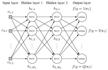
Figure 1: Architecture of the employed DNN.

For phoneme recognition, a DNN is used with the architecture shown in Fig. 1. The DNN’s input is given by 13 MFCC including the $\Delta$ and $\Delta\Delta$ accelerations which are extracted for each frame $\ell$. To these features, a context is added by including the features of the three previous and three future segments which results in the feature vector $\mathbf{v}_{\ell}={[v_{1,\ell},\ldots,v_{V,\ell}]}^{T}$ with dimensionality $V=273$. Here, $v_{i,\ell}$ denote the elements of the feature vector $\mathbf{v}_{\ell}$. Further, $\cdot^{T}$ denotes the vector and matrix transpose. For the employed segment length and segment shift, the context is approximately 100 ms. To improve the robustness of the recognition in noisy environments, the feature vectors are normalized using CMVN [29] before they are employed for training or testing [20]. The CMVN is applied per utterance.

The features are passed through two hidden layers to finally obtain a score $f(q|\mathbf{v}_{\ell})$ for each phoneme $q\in\{1,\ldots,Q\}$. We base the number of phonemes on the annotation given in the TIMIT database [30] which distinguishes between $Q=61$ classes including pauses and non-speech events. The hidden layers of the DNN consist of $H_{1}$ and $H_{2}$ outputs, where $H_{1}=H_{2}=512$ is used. Similar to [31, 32, 20], ReLU are employed as transfer functions of these two layers. For the output layer, a softmax transfer function is used which is interpreted as the posterior probability $f(q|\mathbf{v}_{\ell})$ that phoneme $q$ was spoken given the features $\mathbf{v}_{\ell}$.

0:  Trained DNN and offline computed $\Lambda^{s|q}_{k}$.

0:  Noisy observations ${Y}_{{k,\ell}}$ of a complete utterance.

1:  Extract MFCC $\mathbf{v}_{\ell}$ from ${Y}_{{k,\ell}}$ for complete utterance and add context.

2:  Apply CMVN over complete utterance to give $\mathbf{v}_{\ell}$.

3:  for all segments $\ell$ do

4:     Estimate noise PSD $\hat{\Lambda}^{n}_{k,\ell}$ using [6].

5:     Obtain $f(q|\mathbf{v}_{\ell})$ from the DNN.

6:     for all phonemes $q$ do

7:        Obtain clean speech estimate $\hat{{S}}_{{k,\ell}}^{(q)}$ for phoneme $q$.For this, $\Lambda^{s|q}_{k}$ and $\hat{\Lambda}^{n}_{k,\ell}$ are employed in (2).

8:     end for

9:     Obtain final clean speech estimate $\hat{{S}}_{{k,\ell}}$ using (3).

10:  end for

Algorithm 1 DNN-based enhancement scheme.

For the enhancement, MLSE-based clean speech PSD $\Lambda^{s|q}_{k}$ are employed where each $\Lambda^{s|q}_{k}$ represents the speech PSD of a specific phoneme $q$. During processing, each $\Lambda^{s|q}_{k}$ is used in (2) via $\xi_{{k,\ell}}=\Lambda^{s|q}_{k}/\Lambda^{n}_{k,\ell}$, which yields the phoneme specific clean speech estimates $\hat{{S}}_{{k,\ell}}^{(q)}$. For this, the noise PSD $\Lambda^{n}_{k,\ell}$ is estimated using [6]. Similar to [20], the estimates $\hat{{S}}_{{k,\ell}}^{(q)}$ are averaged based on the recognition scores $f(q|\mathbf{v}_{\ell})$ to give a final estimate $\hat{{S}}_{{k,\ell}}$. More specifically, the clean speech coefficients are obtained by

$$\hat{{S}}_{{k,\ell}}=\sum_{j=1}^{Q}f(q=j|\mathbf{v}_{\ell})\hat{{S}}_{{k,\ell}}^{(q)}.$$ (3)

The steps required to enhance the noisy observations ${Y}_{{k,\ell}}$ using the DNN-based enhancement scheme are summarized in Algorithm 1.

For the training of the DNN-based MLSE system, we employ 1196 gender and phonetically balanced sentences from the TIMIT training set. As in [20], the DNN is trained only using clean speech to ensure that the phoneme recognition does not depend on the background noise type. The target vectors for the training are given by a one-hot encoding of the TIMIT phoneme annotation [30]. The error function is given by the cross-entropy which is minimized using scaled conjugate gradient back-propagation [33]. Before back-propagation, the weights of the DNN’s two hidden layers are initialized using the Glorot method [34]. The weights of the output layer are initialized using the Nguyen-Widrow method [35].

Similar to the non-MLSE-based enhancement scheme, the noise PSD $\Lambda^{n}_{k,\ell}$ is estimated using [6]. The speech PSD $\Lambda^{s|q}_{k}$ that are linked to the phonemes $q$ are obtained as

$$\Lambda^{s|q}_{k}=\frac{1}{|\mathbb{L}^{(q)}|}\sum_{\ell\in\mathbb{L}^{(q)}}|{S}_{{k,\ell}}|^{2},$$ (4)

where $\mathbb{L}^{(q)}$ denotes the set that contains the segments that belong to the phoneme $q$ in the training data. As (4) is scale-dependent, we normalize the time-domain clean speech input signal both in training and testing such that all sentences have the same peak value. During training, the clean speech data is available, while during testing, oracle knowledge is provided. This normalization is also employed for the other enhancement schemes, i.e., for the non-MLSE-based and the NMF-based enhancement scheme given in Section IV. Here, however, the normalization has no influence as these approaches are scale-independent.

IV NMF-Based Speech Enhancement Scheme

In this part, the MLSE-based enhancement scheme that employs NMF is described. It serves as a second example for MLSE-based enhancement schemes. NMF approximates a nonnegative matrix $\mathbf{Y}$ as $\mathbf{Y}\approx\mathbf{{B}}\mathbf{{H}}$, where $\mathbf{{B}}$ and $\mathbf{{H}}$ are also nonnegative matrices. The columns of $\mathbf{{B}}$ are referred to as basis vectors and the columns of $\mathbf{{H}}$ as activation vectors. NMF has been used for source separation, e.g., [36, 37, 22], and has also been applied to speech enhancement, e.g., [38, 39, 40].

Here, a simple, supervised, sparse NMF approach is used which employs the IS divergence as the cost function [22, 23]. As argued in [22], if the noisy spectral coefficients ${Y}_{{k,\ell}}$ are independent and follow a circular-symmetric Gaussian distribution, minimizing the IS divergence for approximating the noisy periodogram as $\left[|{Y}_{{k,\ell}}|^{2}\right]=\mathbf{Y}\approx\mathbf{{B}}\mathbf{{H}}$ allows the elements of the product $\mathbf{{B}}\mathbf{{H}}$ to be interpreted as the noisy PSD $\Lambda^{y}_{k,\ell}$. The IS cost function including the sparsity constraint is given by [23]

$$C=\nu|\mathbf{{H}}|_{1}+\sum_{i,j}\frac{(\mathbf{Y})_{i,j}}{(\mathbf{{B}}\mathbf{{H}})_{i,j}}+\log\left(\frac{(\mathbf{Y})_{i,j}}{(\mathbf{{B}}\mathbf{{H}})_{i,j}}\right)-1,$$ (5)

where $(\cdot)_{i,j}$ denotes element of the respective matrix, $|\cdot|_{1}$ the $L_{1}$-norm, and $\nu$ is the factor that controls the sparsity. This cost function can be optimized using the multiplicative update rules in [23].

For estimating the speech and the noise PSD, it is assumed that the basis matrix $\mathbf{{B}}$ is given by the concatenation of a speech basis matrix $\mathbf{{B}}^{(s)}$ and a noise basis matrix $\mathbf{{B}}^{(n)}$ as $\mathbf{{B}}=[\mathbf{{B}}^{(s)},\mathbf{{B}}^{(n)}]$. The speech and noise basis matrices are learned prior to the processing and are held fixed during processing. This means that only the activation matrices are updated. For obtaining an estimate of $\Lambda^{s}_{k,\ell}$ and $\Lambda^{n}_{k,\ell}$, also the activation matrix $\mathbf{{H}}$ is split into a speech and noise dependent part as $\mathbf{{H}}={[(\mathbf{{H}}^{(s)})^{T},(\mathbf{{H}}^{(n)})^{T}]}^{T}$ such that $\mathbf{Y}\approx\mathbf{{B}}\mathbf{{H}}=[\mathbf{{B}}^{(s)},\mathbf{{B}}^{(n)}]{[(\mathbf{{H}}^{(s)})^{T},(\mathbf{{H}}^{(n)})^{T}]}^{T}$. With this, the speech and the noise PSD can be obtained as

$$\hat{\Lambda}^{s}_{k,\ell} =\sum_{i=1}^{I^{(s)}}(\mathbf{{B}}^{(s)})_{k,i}(\mathbf{{H}}^{(s)})_{i,\ell}$$ (6)

$$\hat{\Lambda}^{n}_{k,\ell} =\sum_{i=1}^{I^{(n)}}(\mathbf{{B}}^{(n)})_{k,i}(\mathbf{{H}}^{(n)})_{i,\ell},$$ (7)

where $I^{(s)}$ is the number of speech basis while $I^{(n)}$ denotes the number of noise bases. The steps for enhancing the noisy observations are summarized in Algorithm 2.

0:  Speech and noise basis matrix $\mathbf{{B}}^{(s)}$, $\mathbf{{B}}^{(n)}$.

1:  Set $\mathbf{{B}}=[\mathbf{{B}}^{(s)},\mathbf{{B}}^{(n)}]$.

2:  for all segments $\ell$ do

3:     Create vector $\mathbf{y}_{\ell}=|{Y}_{{k,\ell}}|^{2}$ and add context.

4:     Initialize $\mathbf{{H}}$ with positive random numbers.

5:     repeat

6:        Update $\mathbf{{H}}$ with the update rule in [23, (4)].

7:     until convergence or maximum iterations reached

8:  end for

9:  Obtain $\hat{\Lambda}^{s}_{k,\ell}$ and $\hat{\Lambda}^{n}_{k,\ell}$ using (6) and (7).

10:  Use estimated PSD in (2) to obtain $\hat{{S}}_{{k,\ell}}$.

Algorithm 2 NMF-based enhancement scheme.

For the NMF-based enhancement scheme, the same speech audio material is employed for training as for the DNN-based enhancement scheme. Also here, a context of 7 segments is employed, i.e., three past and three future segments are appended to the noisy input vectors. As a consequence, the number of rows of the basis matrices is increased and the speech PSD and the noise PSD are reconstructed with a context. For the enhancement, however, only the elements corresponding to the current segment are employed. We use 30 bases in the speech basis matrix $\mathbf{{B}}^{(s)}$ and the noise basis matrix $\mathbf{{B}}^{(n)}$ while the sparsity weight in (5) is set to $\nu=10$.

The noise basis matrices $\mathbf{{B}}^{(n)}$ are trained for a set of specific background noise types. The used types are babble noise, factory 1 noise, and pink noise taken from the NOISEX-92 database [41]. Further, an amplitude modulated version of the pink noise similar to [6] and a traffic noise taken from [42] are included. These noise types are also used later in the evaluation in Section VI. To ensure that different audio material is used in the evaluation, only the first two minutes of the respective noise type are used for training. This corresponds to a partitioning where 50 % of the background noise material is used for training and 50 % for testing. For training and testing, a maximum of 200 iterations are performed for the multiplicative updates in [23]. For testing, the noise matrix appropriate for the respective noise type is chosen in the evaluation, i.e., the background noise type is assumed to be known. The employed non-MLSE-based and the DNN-based enhancement scheme do not require such prior knowledge. However, as discussed in [40, 43], such a supervised approach may be appropriate for some applications, e.g., where the environment can be identified using an environment classifier.

V Importance of Super-Gaussianity for MLSE Based Speech Enhancement

In this section, we analyze the effect of the super-Gaussian speech estimators on non-MLSE-based and MLSE-based speech enhancement schemes. Before that, we analyze how the shape $\mu$ and the compression $\beta$ influence the behavior of MOSIE [1].

V-A Analysis of the Gain Functions

In this part, we analyze the behavior of the clean speech estimator MOSIE [1]. For this, the gain function is considered which is defined as

$$G_{{k,\ell}} =\hat{{S}}_{{k,\ell}}/{Y}_{{k,\ell}}$$ (8)

$$=|\hat{{S}}_{{k,\ell}}|/|{Y}_{{k,\ell}}|.$$ (9)

The equality between (8) and (9) holds due to the fact that MOSIE [1] combines an estimate of the clean speech magnitude $\hat{A}_{{k,\ell}}$ with the noisy phase $\Phi^{y}_{{k,\ell}}$. Thus, the gain is a real-valued function that describes by how much a spectral coefficient is boosted or attenuated depending on the speech PSD $\Lambda^{s}_{k,\ell}$, the noise PSD $\Lambda^{n}_{k,\ell}$, and the noisy input ${Y}_{{k,\ell}}$.

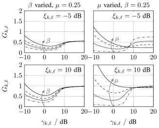
Figure 2: Gain function $G_{{k,\ell}}$ of MOSIE [1] over the a posteriori SNR $\gamma_{{k,\ell}}$ for different values of shape $\mu$ and compression $\beta$. The upper row shows the results for an a priori SNR of -5 dB and the lower for an a priori SNR of 10 dB. See Table I for related estimators for the values of $\mu$ and $\beta$.

Fig. 2 shows the gain $G_{{k,\ell}}$ of MOSIE [1] over the a posteriori SNR $\gamma_{{k,\ell}}$ for two a priori SNR: $\xi_{{k,\ell}}=-5~{}\text{dB}$ is shown in the upper row and $\xi_{{k,\ell}}=10~{}\text{dB}$ in the lower row. The compression parameter $\beta$ is varied and the shape $\mu$ is kept fixed in the left panel and vice versa in the right panel. It is well known that super-Gaussian estimators $(\mu<1)$ preserve speech better than Gaussian estimators $(\mu=1)$ for large a posteriori SNR [13]. However, in the context of MLSE-based speech enhancement, it is of particular interest to observe in Fig. 2 that with decreasing shape $\mu$, a stronger attenuation is applied to the input coefficients for low a posteriori SNR $\gamma_{{k,\ell}}$ even if the a priori SNR $\xi_{{k,\ell}}$ is large. A similar effect is observed if a stronger compression, i.e., smaller values for $\beta$, are employed.

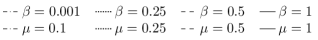
Figure 3: Same as Fig. 2 but over the a priori SNR $\xi_{{k,\ell}}$ and for two fixed a posteriori SNR $\gamma_{{k,\ell}}=0~{}\text{dB}$ and $\gamma_{{k,\ell}}=10~{}\text{dB}$.

These observations are supported by Fig. 3 where the gain function $G_{{k,\ell}}$ is shown over the a priori SNR $\xi_{{k,\ell}}$. Here, the two rows show the behavior for two a posteriori SNR $\gamma_{{k,\ell}}=0~{}\text{dB}$ and $\gamma_{{k,\ell}}=10~{}\text{dB}$. For the Gaussian case ($\mu=1$), Fig. 3 shows that the gain $G_{{k,\ell}}$ mainly depends on the a priori SNR $\xi_{{k,\ell}}$. If the a posteriori SNR $\gamma_{{k,\ell}}$ is close to 0 dB and low values for $\beta$ and $\mu$ are employed, i.e., the super-Gaussian case is considered, the attenuation remains low over a wide range of a priori SNR $\xi_{{k,\ell}}$. Hence, for MLSE-based speech enhancement schemes, the residual noise can be suppressed even for large overestimations of the a priori SNR $\xi_{{k,\ell}}$. This occurs, e.g., between speech spectral harmonics which are not resolved by spectral envelope models.

V-B Effects of Super-Gaussian Estimators on the Enhancement

In this part, we analyze how the behavior of MOSIE [1] influences the considered enhancement schemes. For this, a speech signal taken from the TIMIT test set is corrupted by stationary pink noise at an SNR of 5 dB. The spectrogram of the used signal is shown in Fig. 4. This signal is processed by the non-MLSE-based enhancement scheme and the two MLSE-based enhancement schemes.

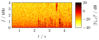
Figure 4: Spectrogram of the example speech signal in stationary pink noise at at 5 dB SNR. Here, $f$ denotes frequency and $t$ time.

In Fig. 5, we depict the resulting a priori SNR $\xi_{{k,\ell}}$. For the DNN-based enhancement scheme, the a priori SNR of the phoneme that is most likely to be present is shown for each segment. Note that this selection is only performed for the visualization in Fig. 5. Otherwise, $\hat{{S}}_{{k,\ell}}$ is estimated as in (3).

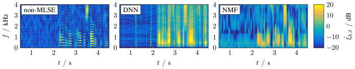
Figure 5: A priori SNR $\hat{\xi}_{{k,\ell}}$ estimated using different enhancement schemes for the excerpt shown in Fig. 4. Here, $f$ denotes frequency and $t$ time.

In Fig. 5, the estimated a priori SNR $\xi_{{k,\ell}}$ obtained from the non-MLSE-based enhancement scheme shows a fine structure which is similar to the speech structure visible in Fig. 4. Contrarily, the structure of the a priori SNR $\xi_{{k,\ell}}$ estimated by the MLSE-based enhancement schemes is very coarse and reveals no or only little of the harmonic fine structure shown in Fig. 4. Using these envelope models for the speech component leads to an overestimation of the a priori SNR $\xi_{{k,\ell}}$ between spectral harmonics.

Next, the gain as defined in (8) is considered. For this example, we use MOSIE [1] with two different parameter setups. First, a setup is used where the clean speech coefficients ${S}_{{k,\ell}}$ are assumed to follow a complex circular-symmetric Gaussian distribution. For this, the parameters of MOSIE [1] are set to $\mu=1$ and $\beta=0.001$, which approximates the Gaussian LSA [4]. For the second setup, the shape is reduced to $\mu=0.2$, i.e., a super-Gaussian LSA is employed. To limit speech distortions, the gain is limited such that attenuations larger than 12 dB are prevented. This limit is applied throughout the paper if not stated otherwise. The applied gains for the Gaussian and super-Gaussian case are shown in Fig. 6.

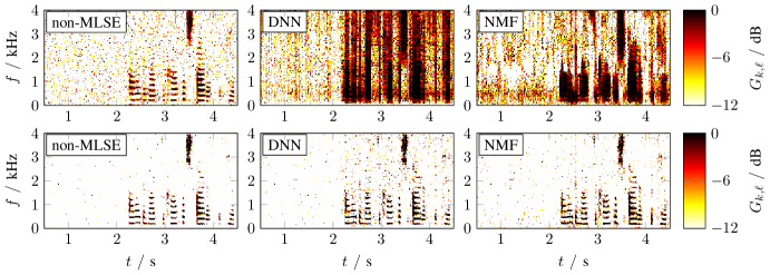
Figure 6: Gain applied to the noisy input coefficients ${Y}_{{k,\ell}}$ by MOSIE [1] for different MLSE-based enhancement schemes for the excerpt shown in Fig. 4. In the upper row, $\mu=1$ and $\beta=0.001$ which approximates the Gaussian LSA proposed in [4] as shown in Table I. In the lower, $\mu=0.2$ and $\beta=0.001$ is used which corresponds to a super-Gaussian LSA. Here, $f$ denotes frequency and $t$ time.

The upper row in Fig. 6 shows that the overestimations of the a priori SNR $\xi_{{k,\ell}}$, e.g., between spectral harmonics, result in a poor suppression for the MLSE-based enhancement schemes when using a Gaussian estimator $(\mu=1)$. The non-MLSE-based enhancement scheme is, however, not affected and achieves high suppression values between harmonics. As discussed in Section V, this behavior can be explained from Fig. 3. For $\mu=1$, the attenuation is mainly controlled by the a priori SNR $\xi_{{k,\ell}}$ where lower a priori SNR $\xi_{{k,\ell}}$ lead to higher suppression values. From this it follows that an overestimation of $\xi_{{k,\ell}}$ results in lower attenuations as observed for the MLSE-based enhancement schemes. As a consequence, using Gaussian clean speech estimators (see Table I) for MLSE-based enhancement schemes results in audible artifacts.

Interestingly, the lower row in Fig. 6 shows that the issues observed for $\mu=1$ can be reduced if a super-Gaussian estimator $(\mu<1)$ is employed. In contrast to Fig. 6, noise is suppressed also between harmonics. Further, also higher attenuations are applied to the noise only segments. Considering Fig. 2 and Fig. 3, the behavior can be explained by the fact that lower shape values cause more suppression for low a posteriori SNR $\gamma_{{k,\ell}}$. Hence, our key conclusion is that using super-Gaussian clean speech estimators, the background noise can be suppressed also when MLSE-based approaches are employed.

VI Instrumental Evaluation

We evaluate the performance of the different speech estimators using instrumental measures such as PESQ improvement scores [44] and SegSNR improvements [14, 45]. The improvements are based on the noisy signal, i.e., they are computed as the difference between the raw scores of the enhanced signal and the noisy signal. Additionally, the SegSSNR and the SegNR [14] are employed to quantify the speech distortions and noise suppression, respectively. Higher values for the SegSSNR indicate less speech distortion and higher values for the SegNR indicates more noise reduction.

For this evaluation, we use 128 sentences from the TIMIT core set. Again, it is ensured that the amount of audio material is balanced between genders. The clean speech signals are artificially corrupted by the same noise types used for training the NMF-based enhancement scheme. The SNR are ranging from -5 dB to 20 dB in 5 dB steps. For each sentence, the segment of the noise signal where the speech signals are embedded in is randomly chosen. The instrumental measures are only evaluated after a two second initialization period to avoid initialization artifacts that may bias the results. Similarly, also the SNR used for the artificial mixing are determined based on the signal powers in speech presence. Further, the noise segments that were used for training the NMF-based enhancement scheme are excluded in the evaluation for all enhancement schemes, i.e., also for the non-MLSE-based and the DNN based enhancement schemes. This is done to make the enhancement schemes more easily comparable.

VI-A Performance Impact of MOSIE’s Parameters

In this section, we analyze how the choice of the shape and the compression parameter influences the performance of clean speech estimators if used for the MLSE-based enhancement schemes.

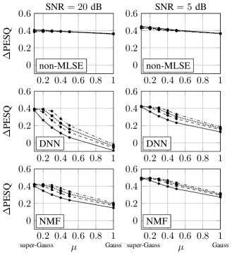
Figure 7: PESQ improvement scores of MOSIE [1] for all considered enhancement schemes in dependence of the shape $\mu$ and compression $\beta$. For relations to other clean speech estimators, see Table I.

Fig. 7 shows the PESQ improvement scores for MOSIE [1] as a function of the shape parameter $\mu$ and the compression parameter $\beta$. The graphs depict the average over all considered noise types and speech files for two different input SNR. For the non-MLSE-based enhancement scheme, increasing super-Gaussianity $(\mu<1)$ and compression $(\beta<1)$ slightly improve the predicted speech quality by PESQ. However, the key message is that for the MLSE-based enhancement schemes, increasing super-Gaussianity ($\mu<1$) and compression ($\beta<1$) improve the signal quality predicted by PESQ considerably stronger.

VI-B Comparison with Common Enhancement Schemes

In this final part of the evaluation section, we compare the super-Gaussian estimators, i.e., MOSIE [1] to Gaussian approaches. To demonstrate that super-Gaussian estimators considerably improve the performance of MLSE-based methods, we use the following two parameter settings for MOSIE [1]: $\beta=0.001,\mu=0.2$ and $\beta=1,\mu=0.2$. The parameters are chosen as a compromise such that all MLSE-based enhancement schemes yield satisfying results.

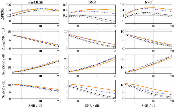
Figure 8: PESQ improvement scores and segmental *SNR measures for different clean speech estimators employed in the non-MLSE-based, the DNN based, and the NMF based enhancement scheme. While LSA and STSA employ Gaussian speech priors, MOSIE ($\mu=0.2,\beta=0.001$) and MOSIE ($\mu=0.2,\beta=1$) represent modern super-Gaussian speech estimators (see Table I).

Fig. 8 shows PESQ improvement scores and segmental SNR measures for the considered enhancement schemes. The results again show that for the non-MLSE-based enhancement scheme, a super-Gaussian estimator only slightly improves the performance. Contrarily, the super-Gaussian setup for MOSIE [1] performs considerably better than the Gaussian clean speech estimator, i.e., the Gaussian STSA [3] and the Gaussian LSA [4], if the MLSE-based estimators are considered. As shown in Section V, the suppression capability of the Gaussian approaches is mainly controlled by the a priori SNR resulting in low suppressions between harmonics for the MLSE-based enhancement schemes where the a priori SNR is overestimated. Here, this is reflected by the low segmental noise reduction values observed for the DNN-based and the NMF-based approach if the Gaussian STSA [3] or the Gaussian LSA [4] are employed. However, for the super-Gaussian estimators MOSIE $(\mu=0.2,\beta=0.001)$ and MOSIE $(\mu=0.2,\beta=1)$ the noise reduction is strongly increased and the residual noise, e.g., the noise between harmonics, is reduced. This comes with a slight increase in speech distortion for MOSIE $(\mu=0.2,\beta=0.001)$ as visible in a decrease in SegSSNR. For MOSIE ($\mu=0.2,\beta=1)$, the SegSSNR remains unchanged or is even slightly increased. Overall, the behavior of the super-Gaussian estimators helps to improve the quality predicted by PESQ and to improve the SegSNR.

VII Subjective Evaluation

As the results of instrumental measures cannot perfectly represent the impressions of human listeners, we verify the results using a subjective listening test. For this, we employ a MUSHRA [46]. In the experiment, two different acoustic scenarios are tested: traffic noise and babble noise both at an SNR of 5 dB. For both acoustic scenarios, an utterance of a male and a female speaker taken from the TIMIT test set are used. These signals are processed by the non-MLSE-based enhancement scheme, the DNN-based enhancement scheme, and the NMF-based enhancement schemes. For all enhancement schemes, a Gaussian STSA ($\mu=1,\beta=1$) and a super-Gaussian STSA ($\mu=0.2,\beta=1$) are compared (see Table I). Even though MOSIE with $\mu=0.2$ and $\beta=0.001$ achieves the highest scores in most instrumental measures, we use MOSIE with $\beta=1$ in the subjective listening test as this configuration produces less musical artifacts.

In each trial, four signals are presented to the listeners: the noisy signals processed by the Gaussian and the super-Gaussian estimator, an anchor, and a hidden reference. The trials are repeated over all combinations of acoustic conditions, speakers and enhancement schemes. The reference signal is a noisy signal with an SNR 17 dB. Finally, for the anchor, the clean speech utterance is filtered using a low-pass filter at a cutoff frequency of 4 kHz and mixed at an SNR of $-5~{}\text{dB}$. This signal is processed using a non-MLSE-based enhancement scheme where the noise PSD is estimated using [6] and the speech PSD is obtained using the decision-directed approach [3] with a smoothing constant set to $0.9$. A Wiener filter with a minimum gain of $-20~{}\text{dB}$ is employed to obtain the anchor. The sound examples used in the experiment are also available at https://uhh.de/inf-sp-tasl2018a.

A total of 13 subjects have participated in the MUSHRA. The test took place in a quiet office and the subjects listened to diotic signals played back through headphones (Beyerdynamic DT-770 Pro 250 Ohm) through a RME Fireface UFX+ sound card. The test was conducted in two phases. In the first phase, the subjects were asked to listen to a subset of the files used in test such that they can familiarize themselves with the different signals. During this training phase, the listeners were also asked to set the level of the headphones to a comfortable level. In the second phase, the listener’s task was to judge the overall quality of the signals on a scale ranging from 0 to 100, where 0 was labeled with “bad” and 100 with “excellent”. The order of presentations of algorithms and conditions were randomized between all subjects.

Figure 9: Box plot of the subjective ratings for different enhancement schemes.

The obtained MUSHRA scores are summarized in Fig. 9 using box plots. The upper and the lower edge of the box show the upper and lower quartile while the bar within the box is the median. The upper whisker reaches to the largest data point that is smaller than the upper quartile plus 1.5 times the interquartile range. The lower whisker is defined analogously. The crosses denote outliers that do not fall in the range spanned by both whiskers. For each box plot, the results of all acoustic conditions and speakers are pooled, which yields 52 data points. The result show that all participants were able to detect the hidden reference, which had to be rated with 100, and that the anchor was consistently given the lowest scores. Further, the results clearly confirm that for the DNN and the NMF based enhancement scheme, the sound quality of the super-Gaussian estimator is considered better than the Gaussian estimator. For the non-MLSE-based estimator, however, the MUSHRA scores of the Gaussian and the super-Gaussian estimator are nearly the same.

Finally, a brief statistical analysis of the results confirms that the differences in MUSHRA scores between the Gaussian and super-Gaussian estimators are statistically significant for the MLSE-based enhancement schemes. For the used statistical tests, a significance level of $\alpha=0.05$ is employed. We apply a Wilcoxon signed-rank test to test for the difference in medians between the MUSHRA scores of the Gaussian and super-Gaussian estimators. This test is employed as the Shapiro-Wilk test indicates that the data is not Gaussian distributed for all conditions. The different enhancement schemes, i.e., the MLSE-based approaches and the non-MLSE-based approach, are treated separately. Considering the difference between the Gaussian and super-Gaussian clean speech estimators for the MLSE-based approaches, the differences are significant in both cases (DNN: $p<0.001$, NMF: $p<0.001$). Comparing the estimators for the non-MLSE-based algorithm reveals no significant difference ($p=0.55$). Hence, the subjective listening tests confirm the previously obtained results of the instrumental measures.

VIII Conclusions

In this paper, super-Gaussian clean speech estimators have been analyzed in the context of machine-learning based speech enhancement approaches that employ spectral envelope models. We refer to these approaches as MLSE. In the analysis part, we showed that the usage of envelope models results in an overestimation of the a priori SNR, e.g., between speech spectral harmonics. As a consequence, using Gaussian estimators, noise between harmonic structures cannot be reduced such that residual noises remain after the enhancement. However, in this paper, we show that employing super-Gaussian clean speech estimators, such as MOSIE [1], leads to a reduction of the undesired residual noise. This interesting result stems from the higher attenuation that is applied by the super-Gaussian estimators if the a posteriori SNR are low. This allows the estimators to compensate for the overestimated a priori SNR without any further post-processing steps. As a consequence, we showed via theoretical analysis and experimental evaluation that for MLSE-based enhancement schemes, super-Gaussian estimators have a much larger effect on improving the enhancement performance than for classic non-MLSE-based enhancement schemes. Sound examples of the considered algorithms are given at https://uhh.de/inf-sp-tasl2018a.

Robert Rehr received his B.Eng. degree from the Jade Hochschule, Oldenburg, Germany, in 2011, and the M.Sc. degree from the Universität Oldenburg, Oldenburg, Germany, in 2013, both in Hearing Technology and Audiology. From 2013 to 2016, he was with the Speech Signal Processing Group at the Universität Oldenburg, Oldenburg, Germany. Since 2017 he has been with the Signal Processing Group at the Universität Hamburg, Hamburg, Germany. R. Rehr is currently pursuing the Ph.D. degree. His research focuses on speech enhancement using machine-learning based methods.

Timo Gerkmann received the Dipl.-Ing. and Dr.-Ing. degrees in electrical engineering and information sciences from the Ruhr-Universität Bochum, Bochum, Germany, in 2004 and 2010 respectively. In 2005, he spent six months with Siemens Corporate Research, Princeton, NJ, USA. From 2010 to 2011, he was a Postdoctoral Researcher in the Sound and Image Processing Laboratory, Royal Institute of Technology (KTH), Stockholm, Sweden. From 2011 to 2015, he was a Professor of speech signal processing with the Universität Oldenburg, Oldenburg, Germany. From 2015 to 2016, he was the Principal Scientist in Audio & Acoustics, Technicolor Research & Innovation, Hanover, Germany. Since 2016, he has been a Professor of signal processing with the University of Hamburg, Hamburg, Germany. His research interests include digital signal processing algorithms for speech and audio applied to communication devices, hearing instruments, audio–visual media, and human–machine interfaces. He is member of the IEEE Signal Processing Society Technical Committee on Audio and Acoustic Signal Processing.

References

- [1] C. Breithaupt, M. Krawczyk, and R. Martin, “Parameterized MMSE Spectral Magnitude Estimation for the Enhancement of Noisy Speech,” in IEEE International Conference on Acoustics, Speech and Signal Processing (ICASSP), Las Vegas, NV, USA, Apr. 2008, pp. 4037–4040.
- [2] M. Krawczyk-Becker and T. Gerkmann, “On MMSE-Based Estimation of Amplitude and Complex Speech Spectral Coefficients Under Phase-Uncertainty,” IEEE/ACM Transactions on Audio, Speech, and Language Processing, vol. 24, no. 12, pp. 2251–2262, Dec. 2016.
- [3] Y. Ephraim and D. Malah, “Speech Enhancement Using a Minimum-Mean Square Error Short-Time Spectral Amplitude Estimator,” IEEE Transactions on Acoustics, Speech, and Signal Processing, vol. 32, no. 6, pp. 1109–1121, Dec. 1984.
- [4] ——, “Speech Enhancement Using a Minimum Mean-Square Error Log-Spectral Amplitude Estimator,” IEEE Transactions on Acoustics, Speech, and Signal Processing, vol. 33, no. 2, pp. 443–445, 1985.
- [5] C. Breithaupt, T. Gerkmann, and R. Martin, “A novel a priori SNR estimation approach based on selective cepstro-temporal smoothing,” in IEEE International Conference on Acoustics, Speech and Signal Processing (ICASSP), Las Vegas, NV, USA, Apr. 2008, pp. 4897–4900.
- [6] T. Gerkmann and R. C. Hendriks, “Noise Power Estimation Based on the Probability of Speech Presence,” in IEEE Workshop on Applications of Signal Processing to Audio and Acoustics (WASPAA), New Paltz, NY, USA, 2011, pp. 145–148.
- [7] C. H. You, S. N. Koh, and S. Rahardja, “ß-Order MMSE Spectral Amplitude Estimation for Speech Enhancement,” IEEE Transactions on Speech and Audio Processing, vol. 13, no. 4, pp. 475–486, Jul. 2005.
- [8] I. Andrianakis and P. R. White, “MMSE Speech Spectral Amplitude Estimators With Chi and Gamma Speech Priors,” in IEEE International Conference on Acoustics, Speech and Signal Processing (ICASSP), vol. 3, Toulouse, France, May 2006, pp. 1068 – 1071.
- [9] J. S. Erkelens, R. C. Hendriks, R. Heusdens, and J. Jensen, “Minimum Mean-Square Error Estimation of Discrete Fourier Coefficients With Generalized Gamma Priors,” IEEE Transactions on Audio, Speech, and Language Processing, vol. 15, no. 6, pp. 1741–1752, Aug. 2007.
- [10] R. C. Hendriks, R. Heusdens, and J. Jensen, “Log-Spectral Magnitude MMSE Estimators under Super-Gaussian Densities,” in Conference of the International Speech Communication Association (Interspeech), Brighton, United Kingdom, 2009, pp. 1319–1322.
- [11] R. C. Hendriks, T. Gerkmann, and J. Jensen, DFT-Domain Based Single-Microphone Noise Reduction for Speech Enhancement: A Survey of the State of the Art, ser. Synthesis Lectures on Speech and Audio Processing. Morgan & Claypool Publishers, 2013, vol. 9, no. 1.
- [12] R. Martin, “Noise Power Spectral Density Estimation Based on Optimal Smoothing and Minimum Statistics,” IEEE Transactions on Speech and Audio Processing, vol. 9, no. 5, pp. 504–512, Jul. 2001.
- [13] ——, “Speech Enhancement Based on Minimum Mean-Square Error Estimation and Supergaussian Priors,” IEEE Transactions on Speech and Audio Processing, vol. 13, no. 5, pp. 845–856, Sep. 2005.
- [14] T. Lotter and P. Vary, “Speech Enhancement by MAP Spectral Amplitude Estimation Using a Super-Gaussian Speech Model,” EURASIP Journal on Advances in Signal Processing, vol. 2005, no. 7, pp. 1–17, 2005.
- [15] Y. Ephraim, “A Bayesian Estimation Approach for Speech Enhancement Using Hidden Markov Models,” IEEE Transactions on Signal Processing, vol. 40, no. 4, pp. 725–735, Apr. 1992.
- [16] D. Burshtein and S. Gannot, “Speech Enhancement Using a Mixture-Maximum Model,” IEEE Transactions on Speech and Audio Processing, vol. 10, no. 6, pp. 341–351, Sep. 2002.
- [17] S. Srinivasan, J. Samuelsson, and W. B. Kleijn, “Codebook Driven Short-Term Predictor Parameter Estimation for Speech Enhancement,” IEEE Transactions on Audio, Speech, and Language Processing, vol. 14, no. 1, pp. 163–176, Jan. 2006.
- [18] D. Y. Zhao and W. B. Kleijn, “HMM-Based Gain Modeling for Enhancement of Speech in Noise,” IEEE Transactions on Audio, Speech, and Language Processing, vol. 15, no. 3, pp. 882–892, Mar. 2007.
- [19] T. Yoshioka and T. Nakatani, “Speech Enhancement Based on Log Spectral Envelope Model and Harmonicity-Derived Spectral Mask, and Its Coupling With Feature Compensation,” in IEEE International Conference on Acoustics, Speech and Signal Processing (ICASSP), Prague, Czech Republic, May 2011, pp. 5064–5067.
- [20] S. E. Chazan, J. Goldberger, and S. Gannot, “A Hybrid Approach for Speech Enhancement Using MoG Model and Neural Network Phoneme Classifier,” IEEE/ACM Transactions on Audio, Speech, and Language Processing, vol. 24, no. 12, pp. 2516–2530, Dec. 2016.
- [21] Q. He, F. Bao, and C. Bao, “Multiplicative Update of Auto-Regressive Gains for Codebook-Based Speech Enhancement,” IEEE/ACM Transactions on Audio, Speech, and Language Processing, vol. 25, no. 3, pp. 457–468, Mar. 2017.
- [22] C. Févotte, N. Bertin, and J.-L. Durrieu, “Nonnegative Matrix Factorization with the Itakura-Saito Divergence: With Application to Music Analysis,” Neural Computation, vol. 21, no. 3, pp. 793–830, Sep. 2008.
- [23] J. Le Roux, F. Weninger, and J. Hershey, “Sparse NMF – half-baked or well done?” Mitsubishi Electric Research Laboratories, Cambridge, MA, USA, Tech. Rep. TR2015-023, Mar. 2015. [Online]. Available: http://www.merl.com/publications/TR2015-023
- [24] R. Rehr and T. Gerkmann, “MixMax Approximation as a Super-Gaussian Log-Spectral Amplitude Estimator for Speech Enhancement,” in Conference of the International Speech Communication Association (Interspeech), Stockholm, Sweden, Aug. 2017.
- [25] J. Hao, T. W. Lee, and T. J. Sejnowski, “Speech Enhancement Using Gaussian Scale Mixture Models,” IEEE Transactions on Audio, Speech, and Language Processing, vol. 18, no. 6, pp. 1127–1136, Aug. 2010.
- [26] N. Mohammadiha, R. Martin, and A. Leijon, “Spectral Domain Speech Enhancement Using HMM State-Dependent Super-Gaussian Priors,” IEEE Signal Processing Letters, vol. 20, no. 3, pp. 253–256, Mar. 2013.
- [27] A. Aroudi, H. Veisi, and H. Sameti, “Hidden Markov model-based speech enhancement using multivariate Laplace and Gaussian distributions,” IET Signal Processing, vol. 9, no. 2, pp. 177–185(8), Apr. 2015.
- [28] C. Breithaupt and R. Martin, “Analysis of the Decision-Directed SNR Estimator for Speech Enhancement With Respect to Low-SNR and Transient Conditions,” IEEE Transactions on Audio, Speech, and Language Processing, vol. 19, no. 2, pp. 277–289, Feb. 2011.
- [29] O. Viikki and K. Laurila, “Cepstral domain segmental feature vector normalization for noise robust speech recognition,” Speech Communication, vol. 25, no. 1–3, pp. 133 – 147, 1998.
- [30] J. S. Garofolo, L. F. Lamel, W. M. Fisher, J. G. Fiscus, D. S. Pallett, N. L. Dahlgren, and V. Zue, “TIMIT Acoustic-Phonetic Continuous Speech Corpus,” 1993.
- [31] L. Tóth, “Phone Recognition with Deep Sparse Rectifier Neural Networks,” in IEEE International Conference on Acoustics, Speech and Signal Processing (ICASSP), Vancouver, BC, Canada, May 2013, pp. 6985–6989.
- [32] G. E. Dahl, T. N. Sainath, and G. E. Hinton, “Improving Deep Neural Networks for LVCSR Using Rectified Linear Units and Dropout,” in IEEE International Conference on Acoustics, Speech and Signal Processing (ICASSP), Vancouver, BC, Canada, May 2013, pp. 8609–8613.
- [33] M. F. Møller, “A Scaled Conjugate Gradient Algorithm for Fast Supervised Learning,” Neural Networks, vol. 6, no. 4, pp. 525 – 533, 1993.
- [34] X. Glorot and Y. Bengio, “Understanding the difficulty of training deep feedforward neural networks,” in International Conference on Artificial Intelligence and Statistics (AISTATS), Chia Laguna Resort, Sardinia, Italy, May 2010, pp. 249–256.
- [35] D. Nguyen and B. Widrow, “Improving the Learning Speed of 2-layer Neural Networks by Choosing Initial Values of the Adaptive Weights,” in International Joint Conference on Neural Networks (IJCNN), San Diego, CA, USA, Jun. 1990, pp. 21–26 vol.3.
- [36] M. N. Schmidt and R. K. Olsson, “Single-Channel Speech Separation using Sparse Non-Negative Matrix Factorization,” in Conference of the International Speech Communication Association (Interspeech), Pittsburgh, PA, USA, Sep. 2006, pp. 1652–1655.
- [37] T. Virtanen, “Monaural Sound Source Separation by Nonnegative Matrix Factorization With Temporal Continuity and Sparseness Criteria,” IEEE Transactions on Audio, Speech, and Language Processing, vol. 15, no. 3, pp. 1066–1074, Mar. 2007.
- [38] N. Mohammadiha, T. Gerkmann, and A. Leijon, “A New Linear MMSE Filter for Single Channel Speech Enhancement Based on Nonnegative Matrix Factorization,” in IEEE Workshop on Applications of Signal Processing to Audio and Acoustics (WASPAA), New Paltz, NY, USA, Oct. 2011, pp. 45–48.
- [39] N. Mohammadiha and A. Leijon, “Nonnegative HMM for Babble Noise Derived From Speech HMM: Application to Speech Enhancement,” IEEE Transactions on Audio, Speech, and Language Processing, vol. 21, no. 5, pp. 998–1011, May 2013.
- [40] N. Mohammadiha, P. Smaragdis, and A. Leijon, “Supervised and Unsupervised Speech Enhancement Using Nonnegative Matrix Factorization,” IEEE Transactions on Audio, Speech, and Language Processing, vol. 21, no. 10, pp. 2140–2151, Oct. 2013.
- [41] H. J. M. Steeneken and F. W. M. Geurtsen, “Description of the RSG.10 noise database,” TNO Institute for perception, Technical Report IZF 1988-3, 1988.
- [42] fxprosound audio design, “Traffic Roadsounds,” Jul. 2009. [Online]. Available: https://www.freesound.org/s/75375/
- [43] N. Mohammadiha, P. Smaragdis, G. Panahandeh, and S. Doclo, “A State-Space Approach to Dynamic Nonnegative Matrix Factorization,” IEEE Transactions on Signal Processing, vol. 63, no. 4, pp. 949–959, Feb. 2015.
- [44] “P.862: Perceptual evaluation of speech quality (PESQ): An objective method for end-to-end speech quality assessment of narrow-band telephone networks and speech codecs,” International Telecommunication Union, ITU-T recommendation, Jan. 2001. [Online]. Available: http://www.itu.int/rec/T-REC-P.862-200102-I/en
- [45] T. Gerkmann and R. C. Hendriks, “Unbiased MMSE-Based Noise Power Estimation With Low Complexity and Low Tracking Delay,” IEEE Transactions on Audio, Speech, and Language Processing, vol. 20, no. 4, pp. 1383–1393, May 2012.
- [46] “BS.1534-3: Method for the subjective assessment of intermediate quality levels of coding systems,” International Telecommunication Union, ITU-T recommendation, Oct. 2015. [Online]. Available: http://www.itu.int/rec/R-REC-BS.1534-3-201510-I/en