Hyperbolicity cones and imaginary projections

Abstract.

Recently, the authors and de Wolff introduced the imaginary projection of a polynomial $f\in\mathbb{C}[\mathbf{z}]$ as the projection of the variety of $f$ onto its imaginary part, $\mathcal{I}(f)\ =\ \{\operatorname{Im}(\mathbf{z})\,:\,\mathbf{z}\in\mathcal{V}(f)\}$. Since a polynomial $f$ is stable if and only if $\mathcal{I}(f)\cap\mathbb{R}_{>0}^{n}\ =\ \emptyset$, the notion offers a novel geometric view underlying stability questions of polynomials. In this article, we study the relation between the imaginary projections and hyperbolicity cones, where the latter ones are only defined for homogeneous polynomials. Building upon this, for homogeneous polynomials we provide a tight upper bound for the number of components in the complement $\mathcal{I}(f)^{\mathsf{c}}$ and thus for the number of hyperbolicity cones of $f$. And we show that for $n\geq 2$, a polynomial $f$ in $n$ variables can have an arbitrarily high number of strictly convex and bounded components in $\mathcal{I}(f)^{\mathsf{c}}$.

1. Introduction

A homogeneous polynomial $f\in\mathbb{R}[\mathbf{z}]=\mathbb{R}[z_{1},\ldots,z_{n}]$ is called hyperbolic in direction $\mathbf{e}\in\mathbb{R}^{n}$ if $f(\mathbf{e})\neq 0$ and for every $\mathbf{x}\in\mathbb{R}^{n}$ the real function $t\mapsto f(\mathbf{x}+t\mathbf{e})$ has only real roots.

We denote by $C(\mathbf{e})=\{\mathbf{x}\in\mathbb{R}^{n}:f(\mathbf{x}+t\mathbf{e})=0\Rightarrow t<0\}$ the hyperbolicity cone of $f$ with respect to $\mathbf{e}$. By Gårding’s results [3], $C(\mathbf{e})$ is convex, $f$ is hyperbolic with respect to every point $\mathbf{e}^{\prime}$ in its hyperbolicity cone and $C(\mathbf{e})=C(\mathbf{e}^{\prime})$ (see [3]). Note, that $0\notin C(\mathbf{e})$ and $-C(\mathbf{e})=C(-\mathbf{e})$ is a hyperbolicity cone of $f$ as well. Furthermore, hyperbolicity cones are open. Recent interest in the hyperbolicity cones was supported by their application in hyperbolic programming (see [4, 10, 12]) as well as by the open conjecture that every hyperbolicity cone is spectrahedral (“Generalized Lax conjecture”, see [16] for an overview as well as [1, 5, 8, 9, 11]).

In [6], the authors and de Wolff introduced the imaginary projection of a polynomial $f\in\mathbb{C}[\mathbf{z}]$ as the projection of the variety $\mathcal{V}(f)$ of $f$ onto its imaginary part, $\mathcal{I}(f)\ =\ \{\operatorname{Im}(\mathbf{z})\,:\,\mathbf{z}\in\mathcal{V}(f)\}$. A polynomial $f\in\mathbb{R}[\mathbf{z}]$ is (real) stable, i.e., its imaginary projection does not intersect the positive orthant, if and only if $f$ is hyperbolic with respect to every point in the positive orthant, see [3, 17]. The complement of the closure of $\mathcal{I}(f)$ consists of finitely many convex components, thus offering strong connections to the theory of amoebas (see [6]).

The main goal of this paper is to study the number of complement components of the imaginary projection of a polynomial $f$. In the homogeneous case, it turns out that this question is equivalent to characterizing the number of hyperbolicity cones of $f$:

Theorem 1.1.

Let $f\in\mathbb{R}[\mathbf{z}]$ be homogeneous. Then the hyperbolicity cones of $f$ coincide with the components of $\mathcal{I}(f)^{\mathsf{c}}$.

Hence, imaginary projections offer a geometric view on the collection of all hyperbolicity cones of a given polynomial. Building upon this, we can provide the following sharp upper bound for homogeneous polynomials.

Theorem 1.2.

Let $f\in\mathbb{R}[\mathbf{z}]$ be homogeneous of degree $d$. Then the number of hyperbolicity cones of $f$ and thus the number of components in the complement of $\mathcal{I}(f)$ is at most

$$\begin{cases}2^{d}&\text{ for }d\leq n\,,\\ 2\sum_{k=0}^{n-1}\binom{d-1}{k}&\text{ for }d>n\,.\end{cases}$$

The maximum is attained if and only if $f$ is a product of independent linear polynomials in the sense that any $n$ of them are linearly independent.

If a part of the boundary of a complement component comes from a linear factor, then the complement component is not strictly convex. It seems to be open whether for given dimension $n$, the number of strictly convex cones in the complement of $\mathcal{I}(f)$ can become arbitrarily large for a homogeneous polynomial $f$. We show in Theorem 1.3, that a non-homogeneous polynomial $f$ can have an arbitrarily large number of strictly convex, bounded components in the complement.

Theorem 1.3.

Let $n\geq 2$. For any $K>0$ there exists a polynomial $f\in\mathbb{R}[\mathbf{z}]$ such that $f$ has at least $K$ strictly convex, bounded components in the complement of $\mathcal{I}(f)$.

The following question remains open:

Question 1.4.

Given a non-homogeneous polynomial $f\in\mathbb{C}[\mathbf{z}]$ of total degree $d$ (or with given Newton polytope $P$), how many bounded or unbounded components can the complement of $\mathcal{I}(f)$ at most have?

The paper is structured as follows. Section 2 deals with the connections of imaginary projections of homogeneous polynomials and hyperbolicity cones and proves Theorem 1.1. Section 3 contains the proof of Theorem 1.2, and it characterizes the boundary of imaginary projections. Section 4 then deals with inhomogeneous polynomials and proves Theorem 1.3.

2. Imaginary projection of homogeneous polynomials and hyperbolicity cones

Throughout the paper, we use bold letters for vectors, e.g., $\mathbf{z}=(z_{1},\ldots,z_{n})\in\mathbb{C}^{n}$. If not stated otherwise, the dimension is $n$. Denote by $\mathcal{V}(f)$ the complex variety of a polynomial $f$ and by $\mathcal{V}_{\mathbb{R}}(f)$ the real variety of $f$. Moreover, set $A^{\mathsf{c}}=\mathbb{R}^{n}\setminus A$ for the complement of a set $A\subseteq\mathbb{R}^{n}$.

For the notion of hyperbolic polynomials, one usually starts from real homogeneous polynomials, while imaginary projections can be defined also for non-homogeneous and for complex polynomials. For coherence, we also consider the notion of a hyperbolic polynomial for complex homogeneous polynomials $f\in\mathbb{C}[\mathbf{z}]$. Note that if $f\in\mathbb{C}[\mathbf{z}]$ is hyperbolic with respect to $\mathbf{a}\in\mathbb{R}^{n}$, then $f(\mathbf{z})/f(\mathbf{a})$ has real coefficients and is hyperbolic with respect to $\mathbf{a}$ as well (see [3]).

For homogeneous polynomials, we now prove the connection between hyperbolicity cones and imaginary projections stated in Theorem 1.1. It generalizes the relation between homogeneous real stable polynomials and hyperbolicity cones, which was already mentioned in the introduction. Note that for a homogeneous polynomial $f$, the imaginary projection $\mathcal{I}(f)$ can be regarded as a (non-convex) cone, i.e., for any $\mathbf{z}\in\mathcal{I}(f)$ and $\lambda\geq 0$ we have $\lambda\mathbf{z}\in\mathcal{I}(f)$. Thus, in particular, $0\in\mathcal{I}(f)$.

Proof of Theorem 1.1.

We show the following two properties:

1. If $f$ is hyperbolic with respect to $\mathbf{e}\in\mathbb{R}^{n}$, then the hyperbolicity cone $C(\mathbf{e})$ satisfies $C(\mathbf{e})\subseteq\mathcal{I}(f)^{\mathsf{c}}$.

2. If there is a convex cone $C$ with $C\subseteq\mathcal{I}(f)^{\mathsf{c}}$, then $f$ is hyperbolic with respect to every point in $C$, i.e., $C$ is contained in that hyperbolicity cone of $f$.

Assume first, that $f$ is hyperbolic with respect to $\mathbf{e}\in\mathbb{R}^{n}$, and let $\mathbf{e}^{\prime}\in C(\mathbf{e})$. Then $\mathbf{e}^{\prime}$ cannot be the imaginary part of a root $\mathbf{z}=\mathbf{x}+i\mathbf{y}$, since otherwise $i$ would be a non-real zero of the univariate function $t\mapsto f(\mathbf{x}+t\mathbf{e}^{\prime})$.

Assume now that there is a convex cone $C$ with $C\subseteq\mathcal{I}(f)^{\mathsf{c}}$. The homogeneity of $f$ implies $-C\subseteq\mathcal{I}(f)^{\mathsf{c}}$. For $\mathbf{e}\in\pm C$, we have $f(\mathbf{x}+i\mathbf{e})\neq 0$ for all $\mathbf{x}\in\mathbb{R}^{n}$, which gives in particular

$$f(\mathbf{e})=(1+i)^{-\deg f}f((1+i)\mathbf{e})=(1+i)^{-\deg f}f(\mathbf{e}+i\mathbf{e})\neq 0,$$

where $\deg(f)$ denotes the degree of the homogeneous polynomial $f$. Furthermore, if there were an $\mathbf{x}\in\mathbb{R}^{n}$ such that $t\mapsto f(\mathbf{x}+t\mathbf{e})$ has a non-real solution $a+ib$, $b\neq 0$, then

$$f(\mathbf{x}+a\mathbf{e}+ib\mathbf{e})=0$$

in contradiction to $b\mathbf{e}\in\pm C\subseteq\mathcal{I}(f)^{\mathsf{c}}$. ∎

As an immediate consequence, we obtain the following description of the imaginary projection of a homogeneous polynomial.

Corollary 2.1.

If $f\in\mathbb{C}[\mathbf{z}]$ is homogeneous, then its imaginary projection is a closed cone (in general non-convex). The components $C_{1},\ldots,C_{t}$ of $\mathcal{I}(f)^{\mathsf{c}}$ are hyperbolicity cones of $f$ and occur pairwise, with $C_{i_{1}}=-C_{i_{2}}$. In particular, the imaginary projection of a homogeneous polynomial has no bounded components in its complement.

Proof.

By Theorem 1.1, the components $C_{1},\ldots,C_{t}$ of $\mathcal{I}(f)^{\mathsf{c}}$ are the hyperbolicity cones of $f$, which occur pairwise. Since hyperbolicity cones are open and since $\mathcal{I}(f)$ has only finitely many of these conic components in the complement, $\mathcal{I}(f)$ is closed. And since $\mathcal{I}(f)$ is a cone, there are no bounded components in the complement. ∎

The following examples illustrate the connection stated in Theorem 1.1 in well-known cases.

Example 2.2.

Let $f(\mathbf{z})=z_{1}\cdots z_{n}$. Then $f$ is hyperbolic with respect to every point $\mathbf{e}\in(\mathbb{R}\setminus\{0\})^{n}$. Setting $z_{j}=x_{j}+iy_{j}$, we obtain

$$\mathcal{I}(f)\ =\ \{\mathbf{y}\in\mathbb{R}^{n}\,:\,\prod_{j=1}^{n}(x_{j}+iy_{j})=0\text{ for some }\mathbf{x}\in\mathbb{R}^{n}\}\ =\ \bigcup_{j=1}^{n}\{\mathbf{y}\in\mathbb{R}^{n}:y_{j}=0\}.$$

Example 2.3.

Let $f(\mathbf{z})=z_{1}^{2}-\sum_{j=2}^{n}z_{j}^{2}$, $n>2$. It is well-known that $f$ is hyperbolic with respect to any point $\mathbf{e}\in\mathbb{R}^{n}$ with $e_{1}^{2}-\sum_{j=2}^{n}e_{j}^{2}>0$ (e.g., [3, Example 1]), and that the two hyperbolicity cones are the open second-order cone (or open Lorentz cone) $\mathcal{L}=\{\mathbf{x}\in\mathbb{R}^{n}\,:\,x_{1}^{2}-\sum_{j=2}^{n}x_{j}^{2}>0,\,x_{1}>0\}$ and its negative $-\mathcal{L}$. Likewise, the imaginary projection of $f$ is $\mathcal{I}(f)=\{\mathbf{y}\in\mathbb{R}^{n}\,:\,y_{1}^{2}-\sum_{j=2}^{n}y_{j}^{2}\leq 0\}=\mathbb{R}^{n}\setminus(\mathcal{L}\cup-\mathcal{L})$, which was computed as part of [6, Theorem 5.4]. This illustrates Theorem 1.1.

Furthermore, if a real homogeneous quadratic polynomial $f\in\mathbb{R}[\mathbf{z}]$ is hyperbolic, then its hyperbolicity cone is the image of the second-order cone under a linear transformation; that property follows from the classification of the imaginary projections of real homogeneous quadratic polynomials in [6].

Example 2.4.

Let $f(\mathbf{z})=\det(z_{1}A_{1}+\dots+z_{n}A_{n})$, where $A_{1},\ldots,A_{n}$ are Hermitian $d\times d$-matrices. It is well-known [9, Prop. 2], that $f$ has the spectrahedral hyperbolicity cone

$$C\ =\{\mathbf{x}\in\mathbb{R}^{n}:x_{1}A_{1}+\dots+x_{n}A_{n}\succ 0\}.$$

This implies that $\pm C$ are components of $\mathcal{I}(f)^{\mathsf{c}}$. We can compute directly that $\mathcal{I}(f)^{\mathsf{c}}$ has exactly these two components. Namely, given some $\mathbf{y}\in\mathbb{R}^{n}$ with $A(\mathbf{y}):=y_{1}A_{1}+\dots+y_{n}A_{n}\succ 0$, we have

(2.1) $$f(\mathbf{x}+i\mathbf{y})=\det\left(\sum_{j=1}^{n}x_{j}A_{j}+iA(\mathbf{y})\right)=\det(A(\mathbf{y}))\cdot\det\left(\sum_{j=1}^{n}x_{j}A(\mathbf{y})^{-1/2}A_{j}A(\mathbf{y})^{-1/2}+iI\right)\,,$$

where $A(\mathbf{y})^{-1/2}$ is the unique matrix with $A(\mathbf{y})^{-1/2}\cdot A(\mathbf{y})^{-1/2}=A(\mathbf{y})^{-1}$. If $f(\mathbf{x}+i\mathbf{y})$ vanished for some $\mathbf{x}\in\mathbb{R}^{n}$, then the Hermitian matrix $\sum x_{j}A(\mathbf{y})^{-1/2}A_{j}A(\mathbf{y})^{-1/2}$ would have the eigenvalue $-i$. But this is impossible, since Hermitian matrices have only real eigenvalues. Hence, $\mathbf{y}\notin\mathcal{I}(f)$.

Conversely, let $f(\mathbf{x}+i\mathbf{y})=0$. Assuming $A(\mathbf{y})\succ 0$, the right hand side of (2.1) vanishes, which again gives the contradiction that $-i$ is an eigenvalue of the Hermitian matrix.

In the following, we consider the number and structure of hyperbolicity cones of a homogeneous polynomial. In order to see that there can appear many hyperbolicity cones, consider polynomials of the form $f(\mathbf{z})=\det(A_{1}z_{1}+\dots+A_{n}z_{n})$ with real diagonal $d\times d$-matrices. This is a special case of Example 2.4, where the spectrahedral hyperbolicity cone becomes a polyhedron. In that case, it becomes profitable to use the viewpoint of imaginary projections to describe exactly the hyperbolicity cones of their complement. Namely, $\mathcal{I}(f)$ is an algebraic variety here, whereas the hyperbolicity cones are semi-algebraic.

Theorem 2.5.

Let $f(\mathbf{z})=\det(A_{1}z_{1}+\dots+A_{n}z_{n})$, where $A_{1},\ldots,A_{n}$ are $d\times d$ real diagonal matrices, $A_{j}=\operatorname{diag}(a_{1}^{(j)},\ldots,a_{n}^{(j)})$. Then $\mathcal{I}(f)$ is the hyperplane arrangement

(2.2) $$\mathcal{I}(f)=\bigcup_{l=1}^{d}\{\mathbf{y}\in\mathbb{R}^{n}:\sum_{j=1}^{n}a_{l}^{(j)}y_{j}=0\}.$$

Lemma 3.1 in Section 3 will show that if $d^{\prime}$ is the number of distinct hyperplanes in (2.2), then the number of complement components is at most $2^{d^{\prime}}$ for $d^{\prime}\leq n$ and at most $2\cdot\sum_{k=0}^{n-1}\binom{d^{\prime}-1}{k}$ for $d^{\prime}>n$.

Proof.

We have

(2.3) $$\det(A_{1}z_{1}+\dots+A_{n}z_{n})=\prod_{l=1}^{d}\left(\sum_{j=1}^{n}a_{l}^{(j)}x_{l}+i\sum_{j=1}^{n}a_{l}^{(j)}y_{l}\right).$$

Assume that there is some $\mathbf{y}\in\mathbb{R}^{n}$ such that $\sum_{j=1}^{n}a_{l}^{(j)}y_{j}=0$ for an $l\in\{1,\ldots,d\}$. Then, choosing $\mathbf{x}=\mathbf{y}$, we have $f(\mathbf{x}+i\mathbf{y})=0$.
Assume now $\sum_{j=1}^{n}a_{l}^{(j)}y_{j}\neq 0$ for all $1\leq l\leq d$. Since (2.3) vanishes if and only if at least one factor vanishes, we have $f(\mathbf{x}+i\mathbf{y})\neq 0$ for all $\mathbf{x}\in\mathbb{R}^{n}$. ∎

We conclude the section with an exact statement on the number of hyperbolicity cones in the bivariate case.

Theorem 2.6.

Let $f\in\mathbb{R}[z_{1},z_{2}]$ be homogeneous and of degree $d$. Then $f$ has at most $2d$ hyperbolicity cones. The exact number depends on the number of distinct solutions of $f(1,z_{2})=0$:

1. If there is at least one complex solution, then there are no hyperbolicity cones.

2. If there are $k$ distinct real solutions, then there are $2k$ hyperbolicity cones.

For the proof, recall the definition of the set of limit directions as the set of limit points of points in $\frac{1}{r}\mathcal{I}(f)\cap\mathbb{S}^{n-1}$ (for $r\to\infty$), written $\mathcal{I}_{\infty}(f)\ =\ \lim_{r\rightarrow\infty}\left(\frac{1}{r}\mathcal{I}(f)\cap\mathbb{S}^{n-1}\right)$, which describes the behavior at infinity of the imaginary projection of a polynomial $f\in\mathbb{C}[\mathbf{z}]$. The following statement was shown in [6, Cor. 6.7].

Proposition 2.7.

Let $f\in\mathbb{C}[z_{1},z_{2}]$ be of total degree $d$ and assume its homogenization $f_{h}\in\mathbb{C}[z_{0},z_{1},z_{2}]$ has the zeros at infinity $(0:1:a_{j})$, $j=1,\ldots,d$. Then

$$\mathcal{I}_{\infty}(f)\ =\ \begin{cases}\bigcup\limits_{j=1}^{d}\left\{\pm\frac{1}{\sqrt{1+a_{j}^{2}}}(1,a_{j})\right\}&\text{if all $a_{j}$ are real,}\\ \mathbb{S}^{1}&\text{otherwise.}\end{cases}$$

Proof of Theorem 2.6..

By Proposition 2.7, either every point on $\mathbb{S}^{1}$ is a limit direction of $f$, or $f$ has at most $2d$ limit directions. Since $f$ is homogeneous, we have $\mathcal{I}_{\infty}(f)=\mathcal{I}(f)\cap\mathbb{S}^{n}$. Hence, every connected component of the complement of $\mathcal{I}(f)\cap\mathbb{S}^{1}$ on the sphere corresponds to a hyperbolicity cone of $f$. The more precise characterization then follows from the more refined characterization in Proposition 2.7 as well. ∎

3. Proof of Theorem 1.2

In this section, we prove Theorem 1.2 on the maximal number of hyperbolicity cones of homogeneous polynomials. Moreover, as a consequence of the results on the hyperbolicity cones, we provide a characterization of the boundary of the imaginary projections of homogeneous polynomials in Theorem 3.5.

For the maximal number of hyperbolicity cones, it will turn out that this number is achieved by polynomials which are products of independent linear factors.

Lemma 3.1.

Let $f(\mathbf{z})=p_{1}(\mathbf{z})\cdots p_{d}(\mathbf{z})\in\mathbb{C}[\mathbf{z}]$ be a product of $d$ linear polynomials $p_{1},\ldots,p_{d}$. Unless $\mathcal{I}(f)=\mathbb{R}^{n}$, the number of hyperbolicity cones of $f$ is positive and at most

1. $2^{d}$ for $1\leq d\leq n,$

2. $2\sum_{k=0}^{n-1}\binom{d-1}{k}$ for $d>n$.

Before the proof, we recall the following statement on linear polynomials from [6], phrased there in the affine setting.

Proposition 3.2.

For every homogeneous linear polynomial $f(\mathbf{z})=\sum_{j=1}^{n}a_{j}z_{j}\in\mathbb{R}[\mathbf{z}]$ with $(a_{1},\ldots,a_{n})\neq 0$, we have $\mathcal{I}(f)=\mathcal{V}_{\mathbb{R}}(\sum_{j=1}^{n}a_{j}y_{j})$. If the coefficients of $f$ are complex, then $\mathcal{I}(f)$ is either a hyperplane or $\mathcal{I}(f)=\mathbb{R}^{n}$.

Proof of Theorem 3.1. Let $f(\mathbf{z})=p_{1}(\mathbf{z})\cdots p_{d}(\mathbf{z})$ be a product of $d$ linear polynomials $p_{1},\ldots,p_{d}$ and $\mathcal{I}(f)\neq\mathbb{R}^{n}$. Since $\mathcal{I}(p_{j})$ is a hyperplane for all $j$, the imaginary projection $\mathcal{I}(f)$ defines a central hyperplane arrangement in $\mathbb{R}^{n}$, where central expresses that all the hyperplanes are passing through the origin. We can assume that the hyperplanes are in general position, since otherwise the number of hyperbolicity cones may only become smaller.

By Zaslavsky’s results [18] (see also [15, Prop. 2.4]), the number of chambers in an affine hyperplane arrangement of $d$ affine hyperplanes in general position is $\sum_{k=0}^{n}\binom{d}{k}$, out of which $\binom{d-1}{n}$ chambers are bounded. Determining the number of chambers in a central hyperplane arrangement of $d$ affine hyperplanes in general position can be reduced to an affine hyperplane arrangement in $\mathbb{R}^{n-1}$ and gives

$$\sum_{k=0}^{n-1}\binom{d}{k}+\binom{d-1}{n-1}\ =\ 2\sum_{k=0}^{n-1}\binom{d-1}{k}\,.$$

For $1\leq d\leq n$, by the Binomial Formula this specializes to the expression given. $\Box$

By the results of Helton and Vinnikov [5], the real variety of a smooth and hyperbolic polynomial consists of nested ovals (and a pseudo-line in case of odd degree) in the projective space $\mathbb{P}^{n-1}$. Hence, the hyperbolicity cone is unique (up to sign). Motivated by an earlier version of the present article, Kummer was able to weaken the precondition and showed that even for irreducible hyperbolic polynomials the hyperbolicity cone is unique (up to sign).

Proposition 3.3 ([7]).

Let $f\in\mathbb{R}[\mathbf{z}]$ be an irreducible homogeneous polynomial. Then $f$ has at most two hyperbolicity cones (i.e., one pair) and thus at most two components in the complement of $\mathcal{I}(f)$.

Lemma 3.4.

Let $f_{1},f_{2}\in\mathbb{C}[\mathbf{z}]$ be homogeneous and $f_{1}$ be irreducible. Then the number of hyperbolicity cones of $f_{1}\cdot f_{2}$ is at most twice the number of hyperbolicity cones of $f_{2}$.

Proof.

First note that any hyperbolicity cone $C$ of $f_{1}\cdot f_{2}$ is of the form $C=C_{1}\cap C_{2}$ with hyperbolicity cones $C_{1}$ and $C_{2}$ of $f_{1}$ and $f_{2}$.

We can assume that $f_{1}$ and $f_{2}$ are hyperbolic. Then, by Theorem 3.3, $f_{1}$ has at most one pair of hyperbolicity cones. Intersecting these two cones with the hyperbolicity cones of $f_{2}$ gives the bound. ∎

Since the lemma inductively extends to an arbitrary number of factors, two or more pairs of hyperbolicity cones only arise from different factors in the polynomial $f$. This fact is captured explicitly by Theorem 1.2, whose proof is now given.

Proof of Theorem 1.2.

Since the case $n=1$ is trivial, we can assume $n\geq 2$. Let $f=p_{1}\cdots p_{k}$ be a homogeneous polynomial of degree $d$, where $p_{1},\ldots,p_{k}$ are irreducible. Hence, $d=\deg(p_{1})+\cdots+\deg(p_{k})$. We construct a polynomial $g=q_{1}\cdots q_{k}$ with linear polynomials $q_{i}$ such that $g$ has at least as many hyperbolicity cones as $f$.

By Lemma 3.4, the number of hyperbolicity cones of $f$ is at most twice the number of hyperbolicity cones of $p_{2}\cdots p_{k}$. Since the irreducible polynomial $p_{1}$ has at most two hyperbolicity cones, there exists some hyperplane $H$ separating these two (open) convex cones. Set $q_{1}$ to be a linear polynomial whose zero set is $H$. The set of hyperbolicity cones of $f$ injects to the set of hyperbolicity cones of $f^{*}=q_{1}p_{2}\cdots p_{k}$. Repeating this process for $p_{2},\ldots,p_{k}$ provides a polynomial $g=q_{1}\cdots q_{k}$ whose number of hyperbolicity cones is at least the number of hyperbolicity cones of $f$.

Hence, the number of hyperbolicity cones is maximized if $f$ is a product of independent linear polynomials. Since replacing any nonlinear polynomial $p_{i}$ by a linear polynomial $q_{i}$ decreases the total degree of the overall product, the maximum number of hyperbolicity cones of a degree $d$ polynomial cannot be attained if $f$ has a nonlinear irreducible factor $p_{i}$.

Now the stated numbers follow from Lemma 3.1. ∎

An illustration, where this number is attained, is given by Theorem 2.5.

For homogeneous polynomials $f$, the uniqueness statement Proposition 3.3 (up to sign) allows to characterize the boundary of $\mathcal{I}(f)^{\mathsf{c}}$ – or equivalently the boundary of the hyperbolicity cones – in terms of the variety $\mathcal{V}(f)$.

Theorem 3.5.

Let $f\in\mathbb{C}[\mathbf{z}]$ be homogeneous. Then

1. $\mathcal{V}_{\mathbb{R}}(f)\subseteq\mathcal{I}(f)$, with equality if and only if $e^{i\phi}f$ is a product of real linear polynomials for some $\phi\in[0,2\pi)$.

2. If $f$ is hyperbolic and irreducible, then the Zariski closure of the boundary of $\mathcal{I}(f)^{\mathsf{c}}$ equals $\mathcal{V}(f)$,

   $$\overline{\partial\mathcal{I}(f)^{\mathsf{c}}}^{Z}=\mathcal{V}(f).$$

Proof.

By homogeneity, if $\mathbf{z}$ is a root of $f$, then $i\mathbf{z}$ is a root of $f$ as well. Hence, if $\mathbf{x}\in\mathcal{V}_{\mathbb{R}}(f)$, then $\mathbf{x}\in\mathcal{I}(f)$.

Let $e^{i\phi}f$ be a linear polynomial with real coefficients. By Proposition 3.2, the imaginary projection of $e^{i\phi}f$ and thus of $f$ is exactly $\mathcal{V}_{\mathbb{R}}(f)$ (notice that $\mathcal{I}(f)\neq\mathbb{R}^{n}$). Hence, the statement holds for products of linear polynomials as well.

For the converse direction, let $\mathcal{I}(f)=\mathcal{V}_{\mathbb{R}}(f)$. Assume first that $f$ is irreducible. We observe that $f$ must be hyperbolic, since otherwise $\mathcal{I}(f)=\mathbb{R}^{n}$, which would imply $f\equiv 0$. By Proposition 3.3, $f$ has exactly one pair of hyperbolicity cones. It corresponds to the two convex, open components $C$ and $-C$ of $\mathcal{I}(f)^{\mathsf{c}}$. By assumption, $\mathcal{I}(f)$ is a real algebraic set, and hence $\mathcal{I}(f)=\partial\mathcal{I}(f)=\partial C=\partial(-C)$. Thus, $\mathcal{I}(f)=\overline{C}\cap\overline{-C}$ is a convex set, where $\overline{C}$ denotes the topological closure of $C$. Since for any two points $\mathbf{a},\mathbf{b}\in\mathcal{I}(f)$ with $\mathbf{a}\neq\mathbf{b}$ their convex combination is contained in $\mathcal{I}(f)=\mathcal{V}_{\mathbb{R}}(f)$, and hence the underlying polynomial must be linear. Due to $\mathcal{I}(f)\neq\mathbb{R}^{n}$, the classification of linear polynomials in [6] (cf. Prop. 3.2 here) provides that $f$ is of the form $e^{i\phi}f$.

If $f$ is a product of non-constant irreducible polynomials, we can consider the imaginary projection of each factor and obtain the overall statement.

For the second statement, let $f$ be hyperbolic with respect to $\mathbf{e}$ and irreducible. By Theorem 1.1, the hyperbolicity cone $C=C(\mathbf{e})$ is a component of $\mathcal{I}(f)^{\mathsf{c}}$. Since $C$ is the connected component in the complement of $\mathcal{V}(f)$ containing $\mathbf{e}$ (see [12]), it is bounded by some subset of its real variety. And since $f$ is irreducible, the Zariski closure of $\partial\mathcal{I}(f)^{\mathsf{c}}$ is $\mathcal{V}(f)$. ∎

4. Non-homogeneous polynomials and their homogenization

In this section, we deal with the complement components for non-homogeneous polynomials as well as with homogenization. For $f\in\mathbb{C}[\mathbf{z}]$, we show that there is a bijection between the set of unbounded components of $\mathcal{I}(f)^{\mathsf{c}}$ with full-dimensional recession cone and the hyperbolicity cones of the initial form of $f$ (as defined below). Then we show Theorem 1.3.

Denote by $f_{h}=f_{h}(z_{0},\mathbf{z})$ the homogenization of $f$ with respect to the variable $z_{0}$. For a set $X\subseteq\mathbb{R}^{n}$ let $\operatorname{cone}X=\{\lambda\mathbf{x}\in\mathbb{R}^{n}\,:\,\mathbf{x}\in X,\lambda\geq 0\}$ denote the cone over $X$. The following statement captures the connection between the imaginary projection of $f$ and the imaginary projection of its homogenization.

Theorem 4.1.

If $f\in\mathbb{C}[\mathbf{z}]$ then $\mathcal{I}(f_{h})\cap\{(y_{0},\mathbf{y})\in\mathbb{R}^{n+1}\,:\,y_{0}=0\}\ =\ \{0\}\times(\operatorname{cone}\mathcal{I}(f)\cup\mathcal{I}(f_{h}(0,\mathbf{z}))).$

Proof.

If $\mathbf{y}$ is a non-zero point in $\operatorname{cone}\mathcal{I}(f)$, we have $\lambda\mathbf{y}\in\mathcal{I}(f)$ for some $\lambda\geq 0$. Hence, there exists an $\mathbf{x}\in\mathbb{R}^{n}$ with $f_{h}((1,\mathbf{x}+i\mathbf{\lambda y}))=0$. By homogeneity of $f_{h}$, this also gives $(0,\mathbf{y})\in\mathcal{I}(f_{h})\cap\{(y_{0},\mathbf{y})\in\mathbb{R}^{n+1}\,:\,y_{0}=0\}$.

Conversely, if $(0,\mathbf{y})$ is a non-zero point in $\mathcal{I}(f_{h})\cap\{(y_{0},\mathbf{y})\in\mathbb{R}^{n+1}\,:\,y_{0}=0\}$ and $y\not\in\mathcal{I}(f_{h}(0,\mathbf{z}))$, then there exists some $\mathbf{x}\in\mathbb{R}^{n}$ and some $c\in\mathbb{R}\setminus\{0\}$ such that $f_{h}((c,\mathbf{x}+i\mathbf{y}))=0$. Hence, $\frac{1}{c}(\mathbf{x}+i\mathbf{y})$ is a zero of $f$, and therefore $\mathbf{y}\in\operatorname{cone}\mathcal{I}(f)$. ∎

By Theorem 4.1, bounded components in the complement vanish under homogenization, and only conic components with apex at the origin remain. Concerning dehomogenization, note that the intersection of the imaginary projection of a homogeneous polynomial $f\in\mathbb{C}[z_{0},\mathbf{z}]=\mathbb{C}[z_{0},\ldots,z_{n}]$ with a fixed hyperplane $\{(y_{0},\mathbf{y})\in\mathbb{R}^{n+1}\,:\,y_{0}=\beta\}$, $\beta\neq 0$ is

$$\mathcal{I}(f_{h})\cap\{(y_{0},\mathbf{y})\in\mathbb{R}^{n+1}\,:\,y_{0}=\beta\}=\bigcup_{\alpha\in\mathbb{R}}\mathcal{I}(f_{h}(\alpha+i\beta,\mathbf{z})).$$

We denote by $\operatorname{in}(f)$ the initial form of $f$, i.e., the sum of all those terms which have maximal total degree. Note that $\operatorname{in}(f)(\mathbf{z})=f_{h}(0,\mathbf{z})$.

Recall that the recession cone of a convex set $A\subseteq\mathbb{R}^{n}$ is $\operatorname{rec}(A)\,=\,\{\,\mathbf{a}\in A\,:\,\mathbf{a}+\mathbf{x}\in A\text{ for all $\mathbf{x}$ in $A$}\}$ (see, e.g., [13]). Whenever $A$ is closed then $\operatorname{rec}(A)$ is closed. For a polynomial $f$, denoting by $\overline{\mathcal{I}(f)}$ the closure of $\mathcal{I}(f)$, we can characterize the components of $(\overline{\mathcal{I}(f)})^{\mathsf{c}}$ with full-dimensional recession cones in terms of the hyperbolicity cones of $\operatorname{in}(f)$.

Theorem 4.2.

For $f\in\mathbb{C}[\mathbf{z}]$, there is a bijection between the set of unbounded components of $\mathcal{I}(f)^{\mathsf{c}}$ with full-dimensional recession cone and the hyperbolicity cones of $\operatorname{in}(f)$.

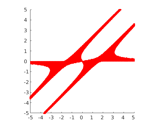
Figure 1. $f(z_{1},z_{2})=z_{1}^{3}-2z_{1}^{2}z_{2}+z_{1}z_{2}^{2}+z_{1}+z_{2}+1$. We have $\operatorname{in}(f)=z_{1}(z_{1}-z_{2})^{2}$, and any boundary point of the complement of $\mathcal{I}(\operatorname{in}(f))$ satisfies $z_{1}=0$ or $z_{1}=z_{2}$. Altogether, $\mathcal{I}(f)^{\mathsf{c}}$ has six components.

Hence, there are at least as many unbounded components in $\mathcal{I}(f)^{\mathsf{c}}$ as components in $\mathcal{I}(\operatorname{in}(f))^{\mathsf{c}}$. Moreover, if $\operatorname{in}(f)$ is hyperbolic, $\mathcal{I}(f)^{\mathsf{c}}$ has at least two (full-dimensional) components. Note that for a polynomial $f$, the terms of lower degree can cause some unbounded components in the complement that have lower-dimensional recession cones. See Figure 1 for an example.

In order to prove the theorem, we show the following lemma, where $\operatorname{int}$ denotes the interior of a set.

Lemma 4.3.

For $f\in\mathbb{C}[\mathbf{z}]$, the following statements hold.

1. The sets of limit directions $\mathcal{I}_{\infty}(f)$ and $\mathcal{I}_{\infty}(\operatorname{in}(f))$ coincide.

2. If $C$ is an unbounded component of $(\overline{\mathcal{I}(f)})^{\mathsf{c}}$ with recession cone $C^{\prime}$, then $\operatorname{int}C^{\prime}$ is a component of $\mathcal{I}(\operatorname{in}(f))^{\mathsf{c}}$ if and only if $\dim C^{\prime}=n$.

3. If $C$ is a component of $\mathcal{I}(\operatorname{in}(f))^{\mathsf{c}}$, then there is a $\mathbf{y}_{0}\in\mathbb{R}^{n}$ such that $\mathbf{y}_{0}+C$ lies in a component of $\mathcal{I}(f)^{\mathsf{c}}$ and $C$ equals the interior of the recession cone of that complement component.

Proof.

(1) The homogenization $f_{h}$ has a zero at infinity, i.e. $(0,z_{1},\ldots,z_{n})\subseteq\mathcal{V}(f_{h})$, if and only if $\operatorname{in}(f)=f_{h}(0,z_{1},\ldots,z_{n})=0$. Hence, the limit directions of $f$ and $\operatorname{in}(f)$ coincide.

(2) Since hyperbolicity cones are open, $\mathcal{I}(\operatorname{in}(f))$ is closed and thus $\mathcal{I}_{\infty}(f)=\mathcal{I}_{\infty}(\operatorname{in}(f))$ is closed as well.

Let $C$ be an unbounded component of $(\overline{\mathcal{I}(f)})^{\mathsf{c}}$ with recession cone $C^{\prime}$. If $\dim C^{\prime}<n$, then $\operatorname{int}C^{\prime}=\emptyset$, hence $C^{\prime}$ is not a hyperbolicity cone of the homogeneous polynomial $\operatorname{in}(f)$. Conversely, if $\dim C=n$ then let $\mathbf{y}_{0}\in\mathbb{R}^{n}$ with $\mathbf{y}_{0}+C^{\prime}\subseteq C$. For all $r>0$ we have

$$\frac{1}{r}\big{(}(\mathbf{y}_{0}+C^{\prime})\cap\mathcal{I}(f)\big{)}\cap\mathbb{S}^{n-1}=\emptyset.$$

Under taking the limit $r\rightarrow\infty$, we obtain that no interior point of the set of limit points

(4.1) $$\lim_{r\rightarrow\infty}\frac{1}{r}(\mathbf{y}_{0}+C^{\prime})\cap\mathbb{S}^{n-1}$$

is a limit direction of $\mathcal{I}(f)$. By (1), these interior points are not limit directions of $\mathcal{I}(\operatorname{in}(f))$ either. As a consequence, $\operatorname{int}C^{\prime}$ is a component of $\mathcal{I}(\operatorname{in}(f))^{\mathsf{c}}$.

(3) Let $C^{\prime}$ be a component of $\mathcal{I}(\operatorname{in}(f))^{\mathsf{c}}$. Set $U=C^{\prime}\cap\mathbb{S}^{n-1}$ and note that the positive hull $\operatorname{pos}U$ satisfies $\operatorname{pos}U=C^{\prime}$. Since $\mathcal{I}(\operatorname{in}(f))$ is a cone, we have $U\subseteq\mathcal{I}_{\infty}(\operatorname{in}(f))=\mathcal{I}_{\infty}(f)$. Hence, there is a $\mathbf{y}_{0}\in\mathcal{I}(f)^{\mathsf{c}}$ such that $\mathbf{y}_{0}+\operatorname{pos}U$ is contained in a component $\mathcal{I}(f)^{\mathsf{c}}$.

Denote by $C^{\prime\prime}$ the recession cone of the component of $\mathcal{I}(f)^{\mathsf{c}}$ that contains $\mathbf{y}_{0}+C^{\prime}$. Clearly, $C^{\prime}\subseteq C^{\prime\prime}$. Using (2), it follows that $\operatorname{int}C^{\prime\prime}=C^{\prime}$. ∎

Theorem 4.2 is a consequence of Lemma 4.3.

Proof of Theorem 4.2. If the recession cone $C^{\prime}$ of $C$ is full-dimensional, then, by Lemma 4.3 (2), $\operatorname{int}C^{\prime}$ is a component of $\mathcal{I}(\operatorname{in}(f))^{\mathsf{c}}$, i.e., $\operatorname{int}C^{\prime}$ is a hyperbolicity cone of $\operatorname{in}(f)$.

Conversely, if the recession cone $C^{\prime}$ of $C$ is a hyperbolicity cone of $\operatorname{in}(f)$, then, by Lemma 4.3 (3), it is open and thus full-dimensional. $\Box$

We now show Theorem 1.3. For $\varphi\in\mathbb{R}$, denote by $R^{\varphi}:\mathbb{R}^{2}\to\mathbb{R}^{2}$ the linear mapping rotating a given point $\mathbf{x}\in\mathbb{R}^{2}$ by an angle $\varphi$ around the origin. $R^{\varphi}$ has a real representation matrix and can also be viewed as a linear mapping $\mathbb{C}^{2}\to\mathbb{C}^{2}$.

Proof of Theorem 1.3.

Given $K\in\mathbb{N}$, we construct a polynomial $p_{K,n}$ in $n$ variables with at least $K$ strictly convex complement components. For the case $n=2$, let

$$g(z_{1},z_{2})\ =\ (-z_{1}^{2}+z_{2}^{2}-1)(z_{1}^{2}-z_{2}^{2}-1)\,,$$

and

(4.2) $$p_{K,2}(\mathbf{z})\ =\ \left(z_{1}^{2}+z_{2}^{2}+r^{2}\right)\cdot\prod_{j=0}^{m-1}g(R_{1}^{2\pi j/m}(z_{1},z_{2}),R_{2}^{2\pi j/m}(z_{1},z_{2}))$$

where $m=\left\lceil\frac{K}{4}\right\rceil$ and $r>0$ sufficiently large. By [6, Thm. 5.3], $\mathcal{I}(z_{1}^{2}+z_{2}^{2}+r^{2})^{\mathsf{c}}$ is the open disk with radius $r$ centered at the origin, and the boundaries of the two-dimensional components of $\mathcal{I}(g)^{\mathsf{c}}$ are given by four hyperbolas. Since the convex components of $\mathcal{I}(g)^{\mathsf{c}}$ and of $\mathcal{I}(z_{1}^{2}+z_{2}^{2}+r^{2})^{\mathsf{c}}$ are strictly convex, the components of $\mathcal{I}(p_{K,2})^{\mathsf{c}}$ are strictly convex. Figure 2 depicts $\mathcal{I}(p_{4,2})$.

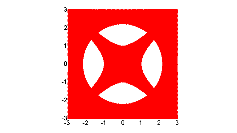
Figure 2. The imaginary projections of $p_{4,2}$.

The expressions $(R^{2\pi j/m}_{1}(z_{1},z_{2}),R^{2\pi j/m}_{2}(z_{1},z_{2}))$ in the arguments of $g$ provide a rotation of its imaginary projection by an angle of $-2\pi j/m$. Choosing $r$ large enough guarantees that the complement component of $\mathcal{I}(z_{1}^{2}+z_{2}^{2}+r^{2})$ is not completely covered by the imaginary projections of the $g(R_{1}^{2\pi j/m}(z_{1},z_{2}),R_{2}^{2\pi j/m}(z_{1},z_{2}))$. Altogether, $\mathcal{I}(p_{K,2})^{\mathsf{c}}$ has $4m\geq K$ bounded and strictly convex, two-dimensional components.

Note that the asymptotes of the hyperbolas do not belong to the imaginary projection of $g$, except the origin. Therefore, $\mathcal{I}(p_{K,2})^{\mathsf{c}}$ has in total $8m$ bounded components.

The case $n\geq 3$ follows by a suitable modification of (4.2). Namely, set

$$g(\mathbf{z})\ =\ (rz_{1})^{2}-\big{(}\sum_{j=2}^{n}z_{j}^{2}\big{)}+1\ =\ r^{2}z_{1}^{2}-\big{(}\sum_{j=2}^{n}z_{j}^{2}\big{)}+1$$

and

$$p_{K,n}(\mathbf{z})\ =\left(\sum_{j=1}^{n}z_{j}^{2}+1\right)\cdot\prod_{j=0}^{m-1}g(R^{2\pi j/m}_{1}(z_{1},z_{2}),R^{2\pi j/m}_{2}(z_{1},z_{2}),z_{3},\ldots,z_{n})\,,$$

where $m=\left\lceil\frac{K}{2}\right\rceil$. $\mathcal{I}(\sum_{j=1}^{n}z_{j}^{2}+1)^{\mathsf{c}}$ is the open ball in $\mathbb{R}^{n}$ with radius $1$ centered at the origin, and by [6, Thm. 5.4] the boundaries of the two convex components of $\mathcal{I}(g)^{\mathsf{c}}$ are given by $B_{1}:=\{\mathbf{y}\in\mathbb{R}^{n}\,:\,y_{1}\geq 1/r\text{ and }r^{2}y_{1}^{2}-\sum_{j=2}^{n}y_{j}^{2}=1\}$ and $B_{2}:=\{\mathbf{y}\in\mathbb{R}^{n}\,:\,y_{1}\leq-1/r\text{ and }r^{2}y_{1}^{2}-\sum_{j=2}^{n}y_{j}^{2}=1\}$. Since $B_{1}\cup B_{2}$ is a two-sheeted $n$-dimensional hyperboloid, $B_{1}$ and $B_{2}$ are the boundaries of strictly convex sets. Note that for $r\to\infty$, the set $\mathcal{I}(g)$ converges to the $y_{1}$-hyperplane on all compact regions of $\mathbb{R}^{n}$.

Again, since the rotation $(R_{1}^{2\pi j/m}(z_{1},z_{2}),R_{2}^{2\pi j/m}(z_{1},z_{2}))$ in the arguments of $g$ induce a rotation of its imaginary projection by an angle of $-2\pi j/m$ with respect to the $y_{1}y_{2}$-plane, choosing $r$ large enough gives $2m\geq K$ bounded and strictly convex components. ∎

5. Conclusion and open question

We have provided quantitative and convex-geometric results on the complement components of imaginary projections and of the hyperbolicity cones of hyperbolic polynomials. In the case of amoebas of polynomials, to every complement component an order can be associated (see [2] for this order map). In the homogeneous case of imaginary projections, the direction vectors of the hyperbolicity cones can be regarded as a (non unique) representative of an order map. And for the unbounded complement components of non-homogeneous polynomials, Theorem 4.2 establishes a connection via the initial form. It is an open question, whether a variant or generalization of this also holds for the bounded complement components in case of non-homogeneous polynomials.

Moreover, Shamovich and Vinnikov [14] recently studied generalizations of hyperbolic polynomials in terms of hyperbolic varieties, and it would be interesting to extend our results to that setting.

References

- [1] N. Amini and P. Brändén. Non-representable hyperbolic matroids. Preprint, arXiv:1512.05878, 2015.
- [2] M. Forsberg, M. Passare, and A. Tsikh. Laurent determinants and arrangements of hyperplane amoebas. Adv. Math., 151(1):45–70, 2000.
- [3] L. Gårding. An inequality for hyperbolic polynomials. J. Math. Mech., 8:957–965, 1959.
- [4] O. Güler. Hyperbolic polynomials and interior point methods for convex programming. Math. Oper. Res., 22(2):350–377, 1997.
- [5] J.W. Helton and V. Vinnikov. Linear matrix inequality representation of sets. Comm. Pure Appl. Math., 60(5):654–674, 2007.
- [6] T. Jörgens, T. Theobald, and T. de Wolff. Imaginary projection of polynomials. Preprint, arXiv:1602.02008, 2016.
- [7] M. Kummer. On the connectivity of the hyperbolicity region of irreducible polynomials. Preprint, arXiv:1704.04388, 2017.
- [8] M. Kummer, D. Plaumann, and C. Vinzant. Hyperbolic polynomials, interlacers, and sums of squares. Math. Program., 153(1, Ser. B):223–245, 2015.
- [9] A. S. Lewis, P. A. Parrilo, and M. V. Ramana. The Lax conjecture is true. Proc. Amer. Math. Soc., 133:2495–2499, 2005.
- [10] Y. Nesterov and L. Tunçel. Local superlinear convergence of polynomial-time interior-point methods for hyperbolicity cone optimization problems. SIAM J. Optim., 26(1):139–170, 2016.
- [11] T. Netzer and R. Sanyal. Smooth hyperbolicity cones are spectrahedral shadows. Math. Program., 153(1, Ser. B):213–221, 2015.
- [12] J. Renegar. Hyperbolic programs, and their derivative relaxations. Found. Comput. Math., 6(1):59–79, 2006.
- [13] R.T. Rockafellar. Convex Analysis. Princeton University Press, Princeton, NJ, 1997.
- [14] E. Shamovich and V. Vinnikov. Livsic-type determinantal representations and hyperbolicity. Preprint, arXiv:1410.2826, 2014.
- [15] R.P. Stanley. An introduction to hyperplane arrangements. In Geometric Combinatorics, volume 13 of IAS/Park City Math. Ser., pages 389–496. Amer. Math. Soc., Providence, RI, 2007.
- [16] V. Vinnikov. LMI representations of convex semialgebraic sets and determinantal representations of algebraic hypersurfaces: past, present, and future. In Mathematical Methods in Systems, Optimization, and Control, volume 222 of Oper. Theory Adv. Appl., pages 325–349. Birkhäuser/Springer Basel AG, Basel, 2012.
- [17] D.G. Wagner. Multivariate stable polynomials: theory and applications. Bull. Amer. Math. Soc., 48(1):53–84, 2011.
- [18] T. Zaslavsky. Facing up to arrangements: face-count formulas for partitions of space by hyperplanes. Mem. Amer. Math. Soc., 1(154), 1975.