Exact solution of an inverse spherical two phase Stefan problem

Merey M. Sarsengeldin^1,2, Abdullah S. Erdogan¹, Targyn A. Nauryz², and Hassan Nouri³

¹ Sigma LABS, ISE, Kazakh-British Technical University, Almaty, Kazakhstan

² Institute of Mathematics and Mathematical Modeling, National Academy of Sciences of Republic of Kazakhstan, Kazakhstan

³ Department of Engineering Design and Mathematics, University of the West of England, Bristol, UK

Abstract In this paper, we represent the exact solution of a two phase inverse spherical Stefan problem, where along with unknown temperature functions heat flux function has to be determined. Suggested solution is obtained from new form of integral error function and its properties which are represented in the form of series whose coefficients have to be determined. The model problem can be used for mathematical modeling and investigation of arc phenomena in electrical contacts.

MSC: 80A22; 33B20

Keywords: Integral error function; Inverse two phase Stefan problem; Electric contacts

1 Introduction

Partial differential equations play an important role for the development of models in heat conduction and investigated in various aspects (see for example [1, 2, 3] and the references therein). To realize the physical changes, some models need to be expressed as free or moving boundary problems. The theory of free boundaries has seen great progress in the last half century. For the general literature up to 2015, we refer to [4, 5]. Present study is devoted to theoretical investigation and mathematical modeling of arc phenomena in electrical contacts and appears as a continuation of recent studies where mathematical modeling of short arcing is considered [6, 7]. Arcing processes are very rapid and include phase transformations like transition therefore it seems reasonable to use Stefan type problems for mathematical modeling of this phenomena.

Worth to say that exact solution of the problem allows to elucidate and enhance understanding of arcing processes and contribute to the development of the arc theory. In the following model heat flux depends on time variable, however, it is well known that besides time variable heat flux depends on numerous factors like electron bombardment and diverse electric contact effects like tunnel, Joule, Thomson, Peltier effects etc. Thus, this model does not claim to be universal for all electric contact phenomena occurring during opening or switching electric contacts.

A long list of studies [10, 11, 12, 13, 14] and literature therein are devoted to Stefan type problems and their solutions. In this study, we consider spherical model which agrees with Holm’s so called ideal sphere usually applied for electric contacts with small contact surface (radius of $b<10^{-4}~{}m$) and low electric current [9]. As it was shown in previous studies this model nicely fits physical conditions and agrees with experimental data [8] where we considered AgCdO and Ni contacts [7].

1.1 Problem Statement

In a spherical model, the contact spot is given by the spherical surface of radius $b$. The heat flux $P(t)$ entering this surface melts the electric contact material (liquid zone $b<r<\alpha(t)$) and then passes further through the solid zone $\alpha(t)<r<\infty$ (for the illustration of the model, see [7, Figure 1]).

The heat equations for each zone are

$$\frac{\partial\theta_{1}}{\partial t}=a_{1}^{2}\left(\frac{\partial^{2}\theta_{1}}{\partial r^{2}}+\frac{2}{r}\frac{\partial\theta_{1}}{\partial r}\right),\quad b<r<\alpha(t),\;t>0,$$ (1)

$$\frac{\partial\theta_{2}}{\partial t}=a_{2}^{2}\left(\frac{\partial^{2}\theta_{2}}{\partial r^{2}}+\frac{2}{r}\frac{\partial\theta_{2}}{\partial r}\right),\quad\alpha(t)<r<\infty,\;t>0$$ (2)

with initial condition

$$\theta_{1}(b,0)=T_{m},$$ (3)

$$\theta_{2}(r,0)=f(r),$$ (4)

$$f(b)=T_{m},\;\alpha(0)=b,\;f(\infty)=0$$ (5)

subjected to boundary condition at $r=b$

$$-\lambda_{1}\frac{\partial\theta_{1}(b,t)}{\partial r} = P(t)$$ (6)

and to free boundary

$$\theta_{1}(\alpha(t),t)=T_{m},$$ (7)

$$\theta_{2}(\alpha(t),t)=T_{m}$$ (8)

the Stefan’s condition

$$-\lambda_{1}\frac{\partial\theta_{1}(\alpha(t),t)}{\partial r}=-\lambda_{2}\frac{\partial\theta_{2}(\alpha(t),t)}{\partial r}+L\gamma\frac{d\alpha}{dt},$$ (9)

as well as the condition at infinity

$$\theta_{2}(\infty,t)=0.$$ (10)

Here $\theta_{1}$ and $\theta_{2}$ are unknown heat functions, $P(t)$ is an unknown heat flux coming from electric arc, $T_{m}$ is a melting temperature of electric contact material, $f(r)$ is a given function and $a_{1}$, $a_{2}$, $\lambda_{1}$, $\lambda_{2}$ and $L\gamma$ are given constants. In the equation, power balance is described by Stefan’s condition $\left(\ref{9}\right)$.

2 Problem Solution

Supposing that the initial and free boundary are analytic functions and can be expanded in Taylor series as

$$f(r)=\sum_{n=0}^{\infty}\frac{f^{(n)}(b)}{n!}(r-b)^{n},\quad\alpha(t)=b+\sum_{n=1}^{\infty}\alpha_{n}t^{n/2},$$ (11)

we represent the solution of $\left(\ref{1}\right)-\left(\ref{10}\right)$ in the following form

$$\theta_{1}(r,t)=\frac{1}{r}\sum_{n=0}^{\infty}(2a_{1}\sqrt{t})^{n}\left[A_{n}i^{n}erfc\frac{r-b}{2a_{1}\sqrt{t}}+B_{n}i^{n}erfc\frac{b-r}{2a_{1}\sqrt{t}}\right],$$

$$\theta_{2}(r,t)=\frac{1}{r}\sum_{n=0}^{\infty}(2a_{2}\sqrt{t})^{n}\left[C_{n}i^{n}erfc\frac{r-b}{2a_{2}\sqrt{t}}+D_{n}i^{n}erfc\frac{b-r}{2a_{2}\sqrt{t}}\right],$$

where coefficients $A_{n},B_{n},\,C_{n}$and $D_{n}$ have to be found.

Lemma 2.1.

The integral error function holds the following properties:

1. $\mathop{\lim}\limits_{x\rightarrow\infty}\frac{i^{n}erfc(-x)}{x^{n}}=\frac{2}{n!},$

2. ${\mathop{\lim}\limits_{t\rightarrow 0}(2a_{1}\sqrt{t})^{n}C_{n}i^{n}erfc\frac{r-b}{2a_{1}\sqrt{t}}=0,}$

3. ${\mathop{\lim}\limits_{t\rightarrow 0}(2a_{1}\sqrt{t})^{n}D_{n}i^{n}erfc\frac{b-r}{2a_{1}\sqrt{t}}=\frac{2}{n!}D_{n}(r-b)^{n}.}$

The proof of the lemma can be given by the L’Hopital’s rule and properties of $i^{n}erfcx$ function.

Theorem 2.2.

Let $f$ be $n$ times differentiable analytic function. Then

$$\lim\limits_{t\rightarrow 0}\theta_{2}(r,t)=\frac{1}{r}\sum_{n=0}^{\infty}\frac{2}{n!}D_{n}(r-b)^{n}.$$

Proof.

Using Lemma 2.1, it is easy to see that

$$\lim\limits_{t\rightarrow 0}\theta_{2}(r,t)=\lim\limits_{t\rightarrow 0}\frac{1}{r}\sum_{n=0}^{\infty}(2a_{2}\sqrt{t})^{n}{D_{n}i^{n}erfc\frac{b-r}{2a_{2}\sqrt{t}}}$$

$$=\frac{1}{r}\lim\limits_{t\rightarrow 0}\sum_{n=0}^{\infty}D_{n}\left(r-b\right)^{n}\frac{{i^{n}erfc}\left(-{\frac{r-b}{2a_{2}\sqrt{t}}}\right)}{\left({\frac{r-b}{2a_{2}\sqrt{t}}}\right)^{n}}=\frac{1}{r}\sum_{n=0}^{\infty}\frac{2}{n!}D_{n}\left(r-b\right)^{n}.$$

∎

2.1 Calculation of coefficients

By the theorem and equations $\left(\ref{4}\right)$ and $\left(\ref{fr}\right)$, we can write

$$\lim\limits_{t\rightarrow 0}\theta_{2}(r,t)=\frac{1}{r}\sum_{n=0}^{\infty}\frac{2}{n!}D_{n}\left(r-b\right)^{n}=f\left(r\right)=\sum_{n=0}^{\infty}\frac{f^{(n)}(b)}{n!}(r-b)^{n}.$$

Thus, we get

$$D_{n}=\frac{1}{2}rf^{(n)}(b).$$

From $\left(\ref{8}\right)$ when we put $r=\alpha(t)$ then $b$ will be canceled and there left only series $\alpha(t)=\alpha_{1}\sqrt{t}+\alpha_{2}t+\alpha_{3}\sqrt{t^{3}}+...=\sum\limits_{n=1}^{\infty}\alpha_{1}t^{n/2}$ in Hartree function if we take $\sqrt{t}$ out of the brackets

$$i^{n}erfc\frac{\sqrt{t}(\alpha_{1}+\alpha_{2}\sqrt{t}+\alpha_{3}t+...)}{2a_{1}\sqrt{t}}=i^{n}erfc\frac{\alpha(t)}{2a_{1}},$$

where

$$\alpha(t)=\alpha_{1}+\alpha_{2}\sqrt{t}+\alpha_{3}t+\cdots=\sum\limits_{n=1}^{\infty}\alpha_{n}t^{\frac{n-1}{2}}.$$

Let’s take $\sqrt{t}=\tau$ and we obtain from equation $\left(\ref{8}\right)$

$$\frac{1}{\alpha(\tau)}\sum_{n=0}^{\infty}(2a_{2}\sqrt{t})^{n}\left[C_{n}i^{n}erfc\delta(\tau)+D_{n}i^{n}erfc(-\delta(\tau))\right]=T_{m},$$ (12)

where $\delta(\tau)=\frac{\alpha(\tau)}{2a_{2}}.$

To calculate coefficient $C_{n}$ we apply Leibniz, Faa Di Bruno’s formulas and Bell polynomials. Using Leibniz formula we have

$$\frac{\partial^{k}[2^{n/2}\tau^{n}i^{n}erfc\delta]}{\partial\tau^{k}}\left|\begin{array}[]{l}\\ {\tau=0}\end{array}\right.=\left\{\begin{array}[]{l}{0,\;for\;k<n}\\ {\frac{2^{n/2}k!}{(k-n)!}[i^{n}erfc\delta]^{(k-n)},\;for\;k\geq n}\end{array}\right..\;$$

Using Faa Di Bruno’s formula and Bell polynomials for a derivative of a composite function we have

$$\frac{\partial^{(k-n)}[i^{n}erfc(\pm\delta)]}{\partial\tau^{k-n}}\left|\begin{array}[]{l}\\ {\tau=0}\end{array}\right.=\sum_{m=1}^{k-n}(i^{n}erfc(\pm\delta))^{(m)}\left|\begin{array}[]{l}\\ {\delta=0}\end{array}\right.B_{k-n,m}(\delta^{\prime(k-n-m+1)}(\tau))|_{\tau=0},$$

where

$$B_{k-n,m}=\sum\frac{(k-n)!}{j_{1}!j_{2}!...j_{k-n-m+1}!}\cdot\beta_{1}^{j_{1}}\beta_{2}^{j_{2}}\beta_{3}^{j_{3}}\cdots\beta_{k-n-m+1}^{j_{k-n-m+1}}$$

and $j_{1},j_{2},\cdots$ satisfy the following equations

$$\begin{array}[]{l}{j_{1}+j_{2}+...+j_{k-n-m+1}=m,}\\ {j_{1}+2j_{2}+...+(k-n-m+1)j_{k-n-m+1}=k-n}\end{array}$$

for $m\geq n$

$$[i^{n}erfc(\pm\delta)]^{(m)}|_{\alpha=0}=(-1)^{m}i^{n-m}erfc0=(\mp 1)^{m}\frac{\Gamma\left(\frac{n-m+1}{2}\right)}{(n-m!)\sqrt{\pi}}$$

by taking both sides of $\left(\ref{14}\right)$ k-times derivatives at $\tau=0$ we have

$$\begin{array}[]{l}{\left\{\sum\limits_{m=1}^{k-p-n}(-1)^{m}\frac{1}{\alpha^{m+1}}\sum\frac{n!\alpha_{1}^{j_{1}}\alpha_{2}^{j_{2}}...\alpha_{n-m+1}^{j_{n-m+1}}}{j_{1}!j_{2}!...j_{n-m+1}!}\,\right\}\cdot\sum\limits_{p=0}^{k}\left(\begin{array}[]{l}{k}\\ {p}\end{array}\right)\left\{\sum\limits_{n=0}^{\infty}\frac{2^{n/2}(k-p)!}{(k-p-n)!}\right.}\\ {\left((-1)^{n}C_{n}\sum_{m=1}^{k-p-n}i^{n-m}erfc\delta_{1}\sum\frac{(k-p)!\delta_{1}^{j_{1}}\delta_{2}^{j_{2}}...\delta_{k-p-n-m+1}^{j_{k-p-n-m+1}}}{j_{1}!j_{2}!...j_{k-p-n-m+1}!}\right.}\\ {\left.\left.{+}D_{n}\sum_{m=1}^{k-p-n}i^{n-m}erfc(-\delta_{1})\sum\frac{(k-p)!\delta_{1}^{j_{1}}\delta_{2}^{j_{2}}...\delta_{k-p-n-m+1}^{j_{k-p-n-m+1}}}{j_{1}!j_{2}!...j_{k-p-n-m+1}!}\right)\right\}=0.}\end{array}$$ (13)

From expression $\left(\ref{15}\right)$ we express coefficients $C_{n}$. From $\left(\ref{7}\right)$ condition we have

$$\frac{1}{\alpha(\tau)}\sum_{n=0}^{\infty}(2a_{1}\sqrt{t})^{n}\left[A_{n}i^{n}erfc\xi(\tau)+B_{n}i^{n}erfc(-\xi(\tau))\right]=T_{m}$$

where

$$\xi(\tau)=\frac{\alpha(\tau)}{2a_{1}}.$$ (14)

As previously by taking both sides of $\left(\ref{16}\right)$ k-times derivatives $\tau=0$ by using Leibniz, Faa Di Bruno’s formulas and Bell polynomials we have

$$\begin{array}[]{l}{\left\{\sum_{m=1}^{k-p-n}(-1)^{m}\frac{1}{\alpha^{m+1}}\sum\frac{n!\alpha_{1}^{j_{1}}\alpha_{2}^{j_{2}}...\alpha_{n-m+1}^{j_{n-m+1}}}{j_{1}!j_{2}!...j_{n-m+1}!}\,\right\}\cdot\sum_{p=0}^{k}\left(\begin{array}[]{l}{k}\\ {p}\end{array}\right)\left\{\sum_{n=0}^{\infty}\frac{2^{n/2}(k-p)!}{(k-p-n)!}\right.}\\ {\left((-1)^{n}A_{n}\sum_{m=1}^{k-p-n}i^{n-m}erfc\xi_{1}\sum\frac{(k-p)!\xi_{1}^{j_{1}}\xi_{2}^{j_{2}}...\xi_{k-p-n-m+1}^{j_{k-p-n-m+1}}}{j_{1}!j_{2}!...j_{k-p-n-m+1}!}\right.}\\ {\left.\left.{+}B_{n}\sum_{m=1}^{k-p-n}i^{n-m}erfc(-\xi_{1})\sum\frac{(k-p)!\xi_{1}^{j_{1}}\xi_{2}^{j_{2}}...\xi_{k-p-n-m+1}^{j_{k-p-n-m+1}}}{j_{1}!j_{2}!...j_{k-p-n-m+1}!}\right)\right\}=0.}\end{array}$$ (15)

We can express from this expression $A_{n}$ coefficient. In Stefan’s condition $\left(\ref{9}\right)$ we take first derivative of

$$\frac{d\alpha}{dt}=\alpha_{1}\frac{1}{2\sqrt{t}}+\alpha_{2}+\frac{3}{2}\alpha_{3}\sqrt{t}+2\alpha_{4}t+...=\sum_{n=1}^{\infty}\frac{n}{2}\alpha_{n}t^{\frac{n-2}{2}}$$

and we take $\sqrt{t}=\tau$

$$\begin{array}[]{l}{\lambda_{1}\frac{1}{\alpha^{2}(\tau)}\sum_{n=0}^{\infty}(2a_{1}\tau)^{n}\left[A_{n}i^{n}erfc\xi(\tau)+B_{n}i^{n}erfc(-\xi(\tau))\right]}\\ {-\lambda_{1}\frac{1}{\alpha(\tau)}\sum_{n=0}^{\infty}(2a_{1}\tau)^{n-1}\left[-A_{n}i^{n-1}erfc\xi(\tau)+B_{n}i^{n-1}erfc(-\xi(\tau))\right]}\\ {=\lambda_{2}\frac{1}{\alpha^{2}(\tau)}\sum_{n=0}^{\infty}(2a_{2}\tau)^{n}\left[C_{n}i^{n}erfc\delta(\tau)+D_{n}i^{n}erfc(-\delta(\tau))\right]}\\ {-\lambda_{2}\frac{1}{\alpha(\tau)}\sum_{n=0}^{\infty}(2a_{1}\tau)^{n-1}\left[-C_{n}i^{n-1}erfc\delta(\tau)+D_{n}i^{n-1}erfc(-\delta(\tau))\right]+\alpha(\tau)L\gamma}\end{array}$$ (16)

where $\alpha(\tau)=\sum_{n=1}^{\infty}\frac{n}{2}\alpha_{n}\tau^{n-2}.$

If multiply both sides of $\left(\ref{18}\right)$ by $\alpha(\tau)$ and using conditions $\left(\ref{7}\right)$,$\left(\ref{8}\right)$ we have the following expression

$$\begin{array}[]{l}{\lambda_{1}\frac{T_{m}}{\alpha(\tau)}-\lambda_{1}\sum_{n=0}^{\infty}(2a_{1}\tau)^{n-1}\left[-A_{n}i^{n-1}erfc\xi(\tau)+B_{n}i^{n-1}erfc(-\xi(\tau))\right]}\\ {=\lambda_{2}\frac{T_{m}}{\alpha(\tau)}-\lambda_{2}\sum_{n=0}^{\infty}(2a_{2}\tau)^{n-1}\left[-C_{n}i^{n-1}erfc\delta(\tau)+D_{n}i^{n-1}erfc(-\delta(\tau))\right]+\beta(\tau)L\gamma,}\end{array}$$ (17)

where

$$\beta(\tau)=\frac{b}{2}\sum_{n=1}^{\infty}n\alpha_{n}\tau^{n-2}+\frac{1}{2}\sum_{n=1}^{\infty}n\alpha_{n}\tau^{2(n-1)}.$$

Previously by taking both sides of $\left(\ref{19}\right)$ k-times derivatives at $\tau=0$ by using Leibniz, Faa Di Bruno’s formulas and Bell polynomials we obtain

$$\begin{array}[]{l}{\left\{\lambda_{1}T_{m}\sum_{m=1}^{k-p-n}(-1)^{m}\frac{1}{\alpha^{m+1}}\sum\frac{n!\alpha_{1}^{j_{1}}\alpha_{2}^{j_{2}}...\alpha_{n-m+1}^{j_{n-m+1}}}{j_{1}!j_{2}!...j_{n-m+1}!}\,\right\}\cdot\sum_{p=0}^{k}\left(\begin{array}[]{l}{k}\\ {p}\end{array}\right)\left\{\sum_{n=0}^{\infty}\frac{2^{n/2}(k-p)!}{(k-p-n-1)!}\right.}\\ {\left((-1)^{n+1}A_{n}\sum_{m=1}^{k-p-n-1}i^{n-m-1}erfc\xi_{1}\sum\frac{(k-p)!\xi_{1}^{j_{1}}\xi_{2}^{j_{2}}...\xi_{k-p-n-m}^{j_{k-p-n-m}}}{j_{1}!j_{2}!...j_{k-p-n-m}!}\right.}\\ {\left.\left.{+}B_{n}\sum_{m=1}^{k-p-n-1}i^{n-m-1}erfc(-\xi_{1})\sum\frac{(k-p)!\xi_{1}^{j_{1}}\xi_{2}^{j_{2}}...\xi_{k-p-n-m}^{j_{k-p-n-m}}}{j_{1}!j_{2}!...j_{k-p-n-m}!}\right)\right\}}\\ {=\left\{\lambda_{2}T_{m}\sum_{m=1}^{k-p-n}(-1)^{m}\frac{1}{\alpha^{m+1}}\sum\frac{n!\alpha_{1}^{j_{1}}\alpha_{2}^{j_{2}}...\alpha_{n-m+1}^{j_{n-m+1}}}{j_{1}!j_{2}!...j_{n-m+1}!}\,\right\}\cdot\sum_{p=0}^{k}\left(\begin{array}[]{l}{k}\\ {p}\end{array}\right)\left\{\sum_{n=0}^{\infty}\frac{2^{n/2}(k-p)!}{(k-p-n-1)!}\right.}\\ {\left((-1)^{n+1}C_{n}\sum_{m=1}^{k-p-n-1}i^{n-m-1}erfc\delta_{1}\sum\frac{(k-p)!\delta_{1}^{j_{1}}\delta_{2}^{j_{2}}...\delta_{k-p-n-m}^{j_{k-p-n-m}}}{j_{1}!j_{2}!...j_{k-p-n-m}!}\right.}\\ {+\left.\left.D_{n}\sum_{m=1}^{k-p-n-1}i^{n-m-1}erfc(-\delta_{1})\sum\frac{(k-p)!\delta_{1}^{j_{1}}\delta_{2}^{j_{2}}...\delta_{k-p-n-m}^{j_{k-p-n-m}}}{j_{1}!j_{2}!...j_{k-p-n-m}!}\right)\right\}+\frac{n!}{2}\left(b\alpha_{k}+\alpha_{k}^{2}\right)L\gamma.}\end{array}$$ (18)

From this recurrent formula we can express $B_{n}$. By using all these expression on condition $\left(\ref{6}\right)$ we express coefficient of heat flux. From $\left(\ref{6}\right)$, we get

$$\begin{array}[]{l}{\frac{\lambda_{1}}{b^{2}}\sum_{n=0}^{\infty}(2a_{1}\sqrt{t})^{n}\left[A_{n}i^{n}erfc0+B_{n}i^{n}erfc0\right]}\\ {\quad\quad+\frac{\lambda_{1}}{b}\sum_{n=0}^{\infty}(2a_{1}\sqrt{t})^{n-1}\left[A_{n}i^{n-1}erfc0-B_{n}i^{n-1}erfc0\right]=\sum_{n=0}^{\infty}P_{n}t^{n/2},}\end{array}$$ (19)

$$\left\{\begin{array}[]{l}{P_{0}=\frac{\lambda_{1}}{b}i^{0}erfc0[A_{1}-B_{1}+\frac{1}{b}A_{0}+\frac{1}{b}B_{0}],}\\ {P_{1}=\frac{\lambda_{1}}{b}(2a_{1})i^{1}erfc0[A_{2}-B_{2}+\frac{1}{b}A_{1}+\frac{1}{b}B_{1}],}\\ {P_{2}=\frac{\lambda_{1}}{b}(2a_{1})^{2}i^{2}erfc0[A_{3}-B_{3}+\frac{1}{b}A_{2}+\frac{1}{b}B_{2}],}\\ \vdots\\ {P_{n}=\frac{\lambda_{1}}{b}(2a_{1})^{n}i^{n}erfc0[A_{n+1}-B_{n+1}+\frac{1}{b}A_{n}+\frac{1}{b}B_{n}].}\end{array}\right.$$

Remark 2.3.

For the convergence of temperature functions $\Theta_{1},\Theta_{2}$, it is possible to follow the idea proposed in [7].

3 Approximate solution of a test problem

To show the effectiveness of the method we proposed the following problem. In this section we show that it is possible to reach $3.5\%$ error using only three points $t_{0}=0$, $t_{1}=0.5$ and $t_{2}=1$ by collocation method which seems to be very practical for engineers.

It is well known that by the help of substitution $\Theta_{i}=\frac{U_{i}}{r}$ it is not difficult to show that spherical heat equation $\frac{\partial\theta_{i}}{\partial t}=a_{i}^{2}\left(\frac{\partial^{2}\theta_{i}}{\partial r^{2}}+\frac{2}{r}\frac{\partial\theta_{i}}{\partial r}\right)$ can be reduced to the well-known heat equation $\frac{\partial u_{i}}{\partial t}=a_{i}\frac{\partial^{2}u_{i}}{\partial x^{2}}$ where $i=1,2$. Thus problem $\left(\ref{1}\right)$-$\left(\ref{10}\right)$ can be reduced to the following problem with slightly modified and simplified boundary conditions without the loss of generality. Solution is found both exactly and approximately. Let us consider

$$\begin{array}[]{l}{\frac{\partial u_{1}}{\partial t}=a_{1}\frac{\partial^{2}u_{1}}{\partial x^{2}},\;0<x<\alpha(t),\;t>0,}\\ {\frac{\partial u_{2}}{\partial t}=a_{2}\frac{\partial^{2}u_{2}}{\partial x^{2}},\;\alpha(t)<x<\infty,\;t>0,}\end{array}$$ (20)

$$u_{1}(0,0)=0,\;\,u_{2}(x,0)=f(x),\text{ }f(0)=u_{m},$$ (21)

$$u_{1}(\alpha(t),t)=u_{2}(\alpha(t),t)=u_{m},$$ (22)

$$u_{1}(0,t)=P(t),$$ (23)

$$-\lambda_{1}\frac{\partial u_{1}}{\partial x}=-\lambda_{2}\frac{\partial u_{2}}{\partial x}+L\gamma\frac{d\alpha}{dt}.$$ (24)

Here $u_{m}$ is a constant and $\alpha(t)=\alpha\sqrt{t}$ is chosen as a moving boundary.

We represent solution of $\left(\ref{22}\right)$-$\left(\ref{26}\right)$ in the following form

$$\begin{array}[]{l}{u_{1}(x,t)=\sum_{n=0}^{\infty}(2a_{1}\sqrt{t})^{n}\left[A_{n}i^{n}erfc\frac{x}{2a_{1}\sqrt{t}}+B_{n}i^{n}erfc\frac{-x}{2a_{1}\sqrt{t}}\right],}\\ {u_{2}(x,t)=\sum_{n=0}^{\infty}(2a_{2}\sqrt{t})^{n}\left[C_{n}i^{n}erfc\frac{x}{2a_{2}\sqrt{t}}+D_{n}i^{n}erfc\frac{-x}{2a_{2}\sqrt{t}}\right],}\end{array}$$

and

$$P(t)=\sum\limits_{n=0}^{\infty}P_{n}(\sqrt{t})^{n},$$

where $P_{n},$ $A_{n},$ $B_{n},$ $C_{n},$ and $D_{n}$ have to be determined. Following the same analogy given in the previous section we find

$$D_{n}=\frac{1}{2}f^{(n)}(0),\;\;n=0,1,2,\cdots,$$ (25)

$$C_{0}=\frac{1}{2}u_{m},$$ (26)

$$C_{n}=-\frac{1}{2}f^{(n)}(0)\frac{i^{n}erfc\frac{-\alpha}{2a_{2}}}{i^{n}erfc\frac{\alpha}{2a_{2}}},$$ (27)

$$A_{0}=\frac{u_{m}-B_{0}erfc\frac{-\alpha}{2a_{1}}}{erfc\frac{\alpha}{2a_{1}}}.$$ (28)

From $\left(\ref{26}\right)$ we get

$$\begin{array}[]{l}{\lambda_{1}(2a_{1})^{-1}\frac{2}{\sqrt{\pi}}\left(-A_{0}\exp\left(\frac{\alpha}{2a_{1}}\right)^{2}+B_{0}\exp\left(-\left(\frac{\alpha}{2a_{1}}\right)^{2}\right)\right)}\\ {=\lambda_{2}(2a_{2})^{-1}\frac{2}{\sqrt{\pi}}\left(-C_{0}\exp\left(\frac{\alpha}{2a_{2}}\right)^{2}+D_{0}\exp\left(-\left(\frac{\alpha}{2a_{2}}\right)^{2}\right)\right)+\frac{L\gamma\alpha}{2}}\end{array}$$ (29)

and from $\left(\ref{24}\right)$ we get

$$A_{n}=-B_{n}\frac{i^{n}erfc\frac{-\alpha}{2a_{1}}}{i^{n}erfc\frac{\alpha}{2a_{1}}}.$$ (30)

Again from Stefan’s condition expressed by equation $\left(\ref{26}\right)$, we get

$$-\lambda_{1}(2a_{1})^{n-1}\left[-A_{n}i^{n-1}erfc\frac{\alpha}{2a_{1}}+B_{n}i^{n-1}erfc\frac{-\alpha}{2a_{1}}\right]$$ (31)

$$= -\lambda_{2}(2a_{2})^{n-1}\left[-C_{n}i^{n-1}erfc\frac{\alpha}{2a_{2}}+D_{n}i^{n-1}erfc\frac{-\alpha}{2a_{2}}\right],$$

$$P_{n-1}=\lambda_{1}(2a_{1})^{n-1}(A_{n}-B_{n})i^{n-1}erfc0,n=1,2,3,\cdots.$$ (32)

Thus coefficients $A_{0},$ $B_{0}$ can be determined from equations $\left(\ref{30}\right)$, $\left(\ref{31}\right)$, coefficients $A_{n},$ $B_{n}$ from $\left(\ref{32}\right)$ and $\left(\ref{33}\right)$,$C_{0},C_{n},D_{n}$ from $\left(\ref{28}\right)$, $\left(\ref{29}\right)$ and $\left(\ref{27}\right)$ respectively and $P_{n}$ from $\left(\ref{34}\right)$.

3.1 Test problem

Let $f(x)=u_{m}+x,\;u_{m}=0,\lambda_{1}=\lambda_{2}=1,a_{1}=a_{2}=1,L=\alpha=\gamma=1$.

We use Mathcad 15 for calculations and get following approximate values for $A_{0}=0.579$, $A_{1}=-3.004$, $A_{2}=-2.333\times 10^{-15}$, $B_{0}=-0.183$, $B_{1}=0.5$, $B_{2}=0$ whereas exact values are $A_{0}=0.604$, $A_{1}=-3.004$, $A_{2}=0$, $B_{0}=-0.191$, $B_{1}=0.5$, and $B_{2}=0$.

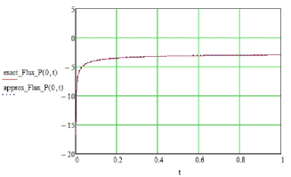
Figure 1: Exact and approximate values of flux function

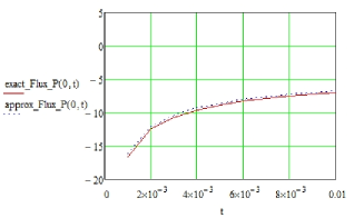
Figure 2: Exact and approximate values of flux function for small t values

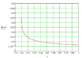
Figure 3: Relative error

In Figures 1 and 2, the graphs of both reconstructed exact (exact_Flux_P(0,t)) and approximate (approx_Flux_P(0,t)) flux functions are shown.

In Figure 3 we illustrate the graph of relative error function calculated by following formula which reaches maximum value $3.5\%$ at point $x=0,~{}0\leq t\leq 1$

$$Error_{rel}=\frac{\left|\text{exact flux-approximate flux}\right|}{\text{exact flux}}.$$

4 Conclusion

A mathematical model describing heat propagation in electric contacts is constructed on the base of two phase spherical inverse Stefan problem. The heat source P(t)is determined from equation $\left(\ref{21}\right)$, which is due to our assumption could be arcing, bridging, Joule heating etc. Temperature functions $\Theta_{1},\Theta_{2}$ which are given in the form of series are determined whose coefficients $\;A_{n},\;B_{n},C_{n}\;$ and $D_{n}$ are also determined from equations $\left(\ref{15}\right)$, $\left(\ref{17}\right)$, $\left(\ref{18}\right)$ and $\left(\ref{20}\right)$. In the test problem we used maximum principle for error estimate, the deviation is 3.5% for three points. For better precision more points has to be taken and better computer characteristics are required.

References

• [1] Jenaliyev, M, Amangaliyeva, M, Kosmakova, M, Ramazanov, M: About Dirichlet boundary value problem for the heat equation in the infinite angular domain. Boundary Value Problems 2014:213, 1-21 (2014).
• [2] Zvyagin, V, Orlov, V: On the weak solvability of one system of thermoviscoelasticity. AIP Conference Proceedings 1676, 020011-1–020011-6 (2015).
• [3] Kavokin, AA, Nauryz, T, Bizhigitova NT: Exact solution of two phase spherical Stefan problem with two free boundaries. AIP Conference Proceedings 1759, 020117-1–020117-4 (2016).
• [4] Friedman, A: Free boundary problems in biology. Phil. Trans. R. Soc. A373:20140368 (2015).
• [5] Chen, G-Q, Shahgholian, H, Vazquez, J-L: Free boundary problems: the forefront of current and future developments. Phil. Trans. R. Soc. A373:20140285 (2015).
• [6] Kharin, SN, Sarsengeldin, M: Influence of contact materials on phenomena in a short electrical arc. In: Khan, S, Salam, I, Ahmed, K (eds.) Key Engineering Materials, vol. 510-511, pp. 321-329. Trans Tech Publications, (2012).
• [7] Sarsengeldin, MM, Kharin, SN: Method of the integral error functions for the solution of the one- and two-phase Stefan problems and its application. Filomat (accepted).
• [8] Kharin, SN, Nouri, H, Davies, T: The mathematical models of welding dynamics in closed and switching electrical contacts. In: Proceedings of 49th IEEE Holm Conference on Electrical Contacts, pp. 107-123, Washington, USA, 2003.
• [9] Holm, R: Electric Contacts. Springer Verlag (1981).
• [10] Friedman, A: Free boundary problems for parabolic equations I. Melting of solids. J. Math. Mech. 8, 499-517 (1959).
• [11] Rubinstein, LI: The Stefan Problem. Transl. Math. Monogr. 27, AMS, Providence, RI (1971).
• [12] Ladyzhenskaya, OA, Solonnikov, VA, Ural’tseva, NN: Linear and Quasilinear Equations of Parabolic Type. Nauka, Moscow (1967).
• [13] Meirmanov, AM: Stefan Problem. Nauka, Novosibirsk (1986).
• [14] Tarzia, DA: A bibliography on moving-free boundary problems for the heat-diffusion equation. The Stefan and related problems. MAT - Ser. A 2, 1–297 (2000).