Separation of time scales and direct computation of weights in deep neural networks
Abstract
Artificial intelligence is revolutionizing our lives at an ever increasing pace. At the heart of this revolution is the recent advancements in deep neural networks (DNN), learning to perform sophisticated, high-level tasks. However, training DNNs requires massive amounts of data and is very computationally intensive. Gaining analytical understanding of the solutions found by DNNs can help us devise more efficient training algorithms, replacing the commonly used mthod of stochastic gradient descent (SGD). We analyze the dynamics of SGD and show that, indeed, direct computation of the solutions is possible in many cases. We show that a high performing setup used in DNNs introduces a separation of time-scales in the training dynamics, allowing SGD to train layers from the lowest (closest to input) to the highest. We then show that for each layer, the distribution of solutions found by SGD can be estimated using a class-based principal component analysis (PCA) of the layer’s input. This finding allows us to forgo SGD entirely and directly derive the DNN parameters using this class-based PCA, which can be well estimated using significantly less data than SGD. We implement these results on image datasets MNIST, CIFAR10 and CIFAR100 and find that, in fact, layers derived using our class-based PCA perform comparable or superior to neural networks of the same size and architecture trained using SGD. We also confirm that the class-based PCA often converges using a fraction of the data required for SGD. Thus, using our method training time can be reduced both by requiring less training data than SGD, and by eliminating layers in the costly backpropagation step of the training.
keywords:
term | term | termArtificial Neural Networks111By neural network, we exclusively mean feed-forward perceptron models. are an integral component of Artificial Intelligence and are recently experiencing a surge in popularity owing to their ability to perform more and more complex and abstract tasks. While many factors, including cheaper computational power and big data, as well as better training algorithms [13], have contributed the revived interest in neural networks, one aspect has remained unchanged in the past fifty years: the use of gradient descent to train a neural network. The major change in recent years has been the ability to train “Deep Neural Networks” (DNN), meaning a network with a large number of layers (tens and sometimes hundreds). In DNN the number of layers is a major contributing factor to the computation time and the amount of data required for training. While training within each layer can be parallelized using GPUs and other hardware, the “backpropagation” step222 “Error Backpropagation” is the term used for the usual chain rule used in computing the gradients of the cost function. cannot, and needs to be performed sequentially. Thus, the following question arises: Can the parameters of layers be derived analytically, without gradient descent? Doing so efficiently would eliminate the need for backpropagation to that layer and would significantly reduce training time.
Given their complex structure and the large number of parameters, it is highly nontrivial how the training of a deep neural network can converge into “good” solutions. Naively speaking, DNNs have a mathematical structure similar to a physical model called spin glass [3, 4, 11], which is a system of binary nodes interacting over a random network. Minimizing the cost function when training a DNN is equivalent to finding the ground state (minimum energy configuration) in a spin glass. Most spin glasses, especially with random interactions, have a very rough energy landscape full of local minima, hence finding the low energy states becomes an NP hard problem. Thus, the question is how do DNNs manage to converge to satisfactory solutions?
Deep networks are much more efficient than shallower networks [29] in certain classification tasks. It is known that lower layers capture general features in the data, and as we make the network deeper, higher layers become more abstract and specific to the label classes [32]. The best example is perhaps the activation pattern of filters in convolutional (ConvNet) layers [20] trained for image classification. As we consider deeper layers, the trained filters represent more and more complex and high-level features in the data [21] constructed by combining lower-level features. But how a network, in which weights of all layers are being updated simultaneously, ends up choosing sensible abstract features at each level is also not fully understood. Note that, while “pre-training” of layers [5, 26] as auto-encoders contributed to the revived success of neural networks, many recent DNNs, such as AlexNet [19] or VGGNET [28], converge without a pre-training step, mainly due to availability of large amounts of training data.
The goal of this paper is to gain analytical understanding of the distribution of solutions that SGD converges to in DNNs trained for classification tasks. We start from the SGD equations and show that with an unbounded activation function, such as the Rectified Linear Unit (ReLU), the widely used –and most successful– Glorot initialization [12] leads to a hierarchy in the rate of dynamics of different layers, with lower layers evolving much faster than higher ones. We show that this “separation of time-scales” allows SGD to solve layers from the lowest to the highest. Additionally, examining SGD for each layer near convergence reveals that the dynamics of different label classes approximately decouple. SGD for each class then becomes a familiar “Langevin equation” [9, 16]. We derive the distribution of solutions for each class, showing that the optimal solution can be found using PCA on the input for that class. We test these findings by creating pre-trained convolutional layers that replace existing layers in networks. On MNIST [22], CIFAR10 [18] and CIFAR100 [18] we observe that our fixed, pre-trained layers perform on par or superior to ConvNet.
1 A word on stochasticity and the learning dynamics
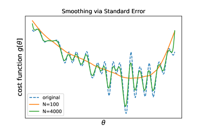
The problem that we will focus on is classification: We wish to map a set of input vectors to output label vectors (assumed to be “one-hot” vectors) using a nonlinear function , where are the parameters (i.e. weights and biases). The function summarizes the action of a neural network with parameters on the data . We discuss the structure of the neural network below. To assess the goodness of fit, we have a cost function , which we write as . The are assumed to be bounded. The goal is to find such that the cost is minimized. is also assumed to be smooth, except on a set of measure zero. The standard method for training DNNs is SGD. In SGD, data is processed gradually in mini-batches. In early steps, the will have stochastic fluctuations of order , with being the number of data inputs processed. Given a cost function with a set of parameters (weights and biases ), the standard error defines a resolution limit for SGD at step : local minima in the landscape of whose widths are smaller than , ( is the standard deviation of ) are invisible to SGD because stochastic fluctuations are large enough to make escape such local minima (SI Fig. 1). An important consequence of this is that, much like temperature in simulated annealing [17], standard error results in an effective “smoothing” of the energy landscape in SGD in the usual sense of “Kernel Density Estimation” [10, 31], forcing it to find a low energy (cost) local minimum in the smoothened landscape of . As SGD progresses, the standard error diminishes and narrow local minima become resolvable. Near the bottom of the smoothened minimum stochastic fluctuations dominate and the gradient becomes negligible. Thus, SGD will have two phases: 1) A “fast drift phase” driven by strong gradients, with a consistent direction; 2) A “relaxation phase” near the bottom of a local minimum333Note that these phases may occur multiple times as different layers may be entering this phase at different times and the landscape becomes less smooth during SGD.. These two phases were observed and utilized by [27] where the fast drift phase is described as a “representation compression” phase. Fig. 1 shows an actual SGD for a convex to illustrate the two phases. Note that these two behaviors are a quite general feature of any stochastic process, such as diffusion, happening on an energy landscape with local minima.
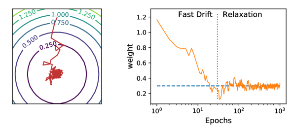
We show below that the fast drift phase can lead to a “separation of time scales”: Layers closer to data have much faster dynamics than layers above them. The condition for this to happen is having an activation function which is unbounded from above and a suitable initialization, e.g. Rectified Linear Units (ReLU) with Glorot initialization [12, 14]. When the system enters the relaxation phase, this separation of time scales still exists and we can utilize it to considerably simplify the SGD equations. The relaxation phase is a period where the gradients mostly vanish and the dynamics is dominated by stochastic fluctuations. The system will be fine-tuning to find the exact position of the local minimum, as the details of landscape of become resolvable. It is important to note that each layer may enter the relaxation phase at a different time step. We will exploit this to analytically derive the distribution of weights. We will now delve into the details of the setup of the problem and the SGD equations.
2 Setup and notation
We consider the classification problem of labeling input images with one-hot vectors as output labels. We want to achieve this task using an layer neural network defined below. The dimension of the output, or number of output “channels”, of layer is denoted by . The labels have dimension equal to the number of classes . The output of layer of the network is where is the “activation function” and , which we call the “raw output”. and are called the “weights” and “biases” of layer , respectively. refers to channel of the output of layer , for the th input. Thus, is the input and is the corresponding output of the network.
| Symbol | Notation |
|---|---|
| # of layers | |
| # of training data | |
| # of label classes | |
| dimension of layer output | |
| the th input image | |
| label for input th | |
| weights of layer | |
| bias of layer , channel | |
| output of layer , channel , image |
2.1 Activation Functions
While in the past nonlinear bounded functions such as tanh and sigmoid were commonly used as activation functions, most recent DNN architectures favor ReLU activation, defined simply as . The preference for ReLU is due to a number of reasons including lower computational complexity, constant gradient, faster learning, and a reduced likelihood of vanishing gradient problem [6, 24]. We will consider a feed-forward network, with the first layers having ReLU activation function444Note that, although ReLU is not a smooth function, it won’t cause any problems in SGD because the non-smoothness is on a set of measure zero and discrete methods such as SGD will never discover the non-smooth part of the domain. . The last layer is the classification layer with number of hidden nodes equal to the number of classes (i.e. ) and a softmax activation function defined below. Table 1 summarizes our notation. In most of what follows, we will only show the layer index and sometimes the input index . Matrix multiplication is implied unless stated otherwise. With ReLU, the output of layer can be written as
| (1) |
where is the Heaviside step function and is a diagonal matrix with on the leading diagonal. For the classification layer, we choose a softmax activation function, defined as , with the normalization factor being the sum over classes .
2.2 Cost Function
In classification problems, categorical cross-entropy provides a natural cost function for softmax activation function, as it measures the Kullback-Leibler divergence between the distribution of outputs and labels
| (2) |
2.3 Gradient Descent with ReLU
Gradient descent consists of changing the weights and biases opposite to the gradient of the cost function to find minima. The number of processed data points defines the time step of SGD in neural networks555During training, data points are also reused. After one “epoch”, i.e. after processing all training data once, the mini-batches are randomly sampled from the data set again. For our purpose, we may treat reused data after the first epoch as new data. We will not make a distinction between the different epochs. . When a new mini-batch of size is processed, the weights and biases will be changed according to
| (3) |
where is the learning rate, which can be dynamically adjusted, and . The components of gradient of the cost function are
| (4) |
where we have used the fact that and defined
| (5) |
We wish to understand the dynamics of (4). The factors that depend on in (4) are the weights of higher layers through and the output of the previous layer . We will show below that with ReLU the Frobenius norm of will be larger for smaller . For , we will show that it will contain competing terms and together with the nonlinearity from ReLU, will not have a clear factor of weights and biases like .
3 Fast drift phase and singular values of
It is known that initial values of the weights affect the accuracy of DNNs significantly [14]. For ReLU, the best performing initialization scheme is found to be the Glorot method [12, 14] which limits the variance of weights so that the initial singular values of initial weights are equal to two. We will now show that Glorot initialization leads to a separation of time scales because it will result in acquiring singular values (SV) which are greater than and which are larger for smaller . Fig. 2 shows experimental evidence supporting this claim in a test network consisting of four dense layers666The exact architecture is: Maxpool (3,3), Dense(30), Dense(100), Dense(30), Classification(10). The dense layers have about 3000 trainable parameters, while the classification layer has 310. trained on the MNIST dataset. It shows that of all layers quickly acquire SV and that the product , as a proxy for , has larger maximum SV for smaller . In Glorot Initialization, all weights are initialized as random Gaussian (normal) distributions with variance . This sets all SVs of to (SI, eq. (30); see also [12]).
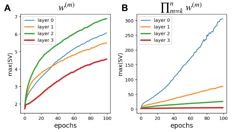
Now consider the combination which appears in . Because the initialization is random Gaussian, the rows of the raw outputs are equally likely to be positive and negative, meaning half of the rows of are zero. Therefore, the SVs of are initialized to and so all SVs of are also initially (SI eq.(30)). The SVs of are the square-root of eigenvalues of . In early steps, rows of are uncorrelated and so (SI, eq.(31)). As discussed earlier, because of standard error, which for at step becomes , SGD cannot resolve sharp minima in early stages and the dynamics effectively occurs on a smoothened landscape of with local minima that are wider and far less abundant than in without this smoothing. In early stages, and, therefore, the smoothened local minima have width . Since in early stages, the gradient is not random and has non-zero magnitude, it maintains a consistent direction in the dimensions. The gradient will, therefore, move the mean of columns away from zero to . The largest SV of is the square-root of the largest eigenvalue of which in early stages with yields
| (6) |
In other words, while the Glorot initialization is exactly tuned to set the initial SVs of equal to one, it also guarantees that the SVs become larger than one in early stages of SGD. We will argue that this is essential in allowing SGD to solve layers one by one. The immediate consequence of this is that will be larger for smaller , as it contains factors of weights, each with some SVs larger than one. Because of the multiplication of weights in , the gradients of biases in (4) are much larger for lower layers. The weight gradients (4) also contain another factor , which we will discuss now.
3.1 Magnitude of
Note that we cannot yet conclude that the norm of the weight gradients is larger for lower layers because of the factor in (4). One may argue that contains the product of the weights of the first layers and therefore the gradients of for all are of the same magnitude. But it is easy to see that cannot remain . To see this, we examine the change in after processing a minibatch during SGD. Using (3)–(4), we have
| (7) | ||||
| (8) |
Thus, SGD will change by terms proportional to . Therefore in (4) will not have a well-defined factor of weights and, in particular, cannot consistently remain close to .
In conclusion, the only factor of weights that is guaranteed to be present in the evolution of weights (and biases) is the in (4). As we showed above, has larger maximum SV for smaller , resulting in lower layers having gradients which are larger than the layer above them by a factor larger than one. The significance of this is that it signals the existence of a “separation of time scales”: the dynamics of lower layers is much faster than the layers above them. This is a point worth deliberating because it means that the dynamics of layers approximately decouple and SGD in layer may effectively ignore dynamics of layer , allowing SGD to solve lower layers without much disruption from higher layers. We will exploit this observation to solve the distribution of weights analytically.
In the end, note that both ReLU and the initialization of weights played a role in this result. Sigmoid or tanh activation would not have resulted in growing SVs and the time scale of evolution of all layers would have been similar. Additionally, the Glorot initialization seems to be the only initialization for ReLU which both makes sure the output of the layer is not exploding initially, while also being guaranteed to lead to SVs larger than one.
4 Relaxation phase
For each layer, when the parameters are in the vicinity of a local minimum, the fast drift phase ends and the layer enters the stochastic relaxation phase. This phase sets in when weights are trained to a good degree and so the gradients and become very small. From Eq. (4), this means that must be small. Using (2), for input
| (9) |
Since the gradient is very small, we can expand the exponential inside as a Taylor series777Note, can be large, but it’s always finite.. First, we make the following -dependent variable redefinition
| (10) |
where we replace the zeros in with a small positive to make well-defined. Define the projection matrix onto class of as . Expanding (9), we have
| (11) |
To further simplify this, we define the “optimal input” as the input that would produce exactly the output vector . In practice, can be constructed via activation maximization [25]. To be precise
| (12) |
where summarizes propagation through the network. Note that is not unique for many reasons including nonlinearity of the network, as well as weights not being full-rank. Let denote the raw output of layer after propagating through the network. We can always find such that the activation patterns of and are similar, meaning . This means that we choose such that it uses features similar to in each layer. This ensures that will be the same for and 888This is a reasonable assumption as we are close to convergence and we can always find an which is close enough to so that this is satisfied.. Defining , we get
| (13) |
where bias-dependent terms exactly cancel. Plugging (13) into (11) and substituting in (4), the weight gradients become
| (14) | ||||
| (15) |
Note that, while is the actual -th input, is the best guess for what input would yield output based on information in the previous data points. Since produces exactly the same redefined label for all we have , which results in the first points canceling in (15)
| (16) |
which also makes use of the fact that in the relaxation phase the weights are close to their locally optimal value. Eq. (16) is a stochastic equation, but the distribution of its solutions can be calculated.
4.1 Estimating distribution of weights for low layers
is similar to a projection onto label , which is a one-hot vector that is nonzero only for some class . But different inputs belonging to the same class may still have very different activation patterns in different layers because they may contain different low and high level features. As a result, can be different for inputs belonging to the same class. But it is also likely that there are groups in inputs for each class such that within each group the activation patterns are the same (i.e. all inputs in one group use exactly the same low and high level features) and so have exactly the same . For such a group of inputs within a class , will be exactly the same, allowing further simplification of (15). However, since we do not know a priori what groups of inputs use the same features, even though these groups exist, we lack the information needed to perform such grouping. So, in the most general case, there does not seem to be any option other than methods like SGD to solve (15).
Despite the above-mentioned problem, in many datasets with refined labels most inputs of the same class share characteristic features. For instance, in the MNIST dataset of handwritten digits with 10 labels all inputs of the class of number 1 contain vertical lines which are less common in other numbers. Therefore, the average of over class 1 will be a good approximation of the characteristic of this class, and it will be different from of other classes. Thus, if for most inputs within class , we could ignore the variability of the activation pattern , we could define a single, averaged , denoted by , for the whole class . In (15), since all inputs of the same class have the same , we can break the sum over down to summations over classes. First, define the “density matrix”999 When are mean zero, the density matrix is just the covariance matrix. for each class as
| (17) |
In (16) is the guessed input based on the previous inputs and it can be expressed as a linear combination101010Note, may be overcomplete and not be linearly independent, but only needs to map onto a linearly independent subset of them. of previous inputs which belonged to the same class as the last label . The last input , on the other hand, contains new information and cannot be an orthogonal transformation of the previous data. Using this, we can show explicitly (SI eq.(38)) that
| (18) |
And so using (16) the SGD equations for the weights become
| (19) |
In the relaxation phase fluctuates mostly due to statistical fluctuations in the data. As every input is an independent drawing from the dataset, is the sum of observations . Since mean and variance of the input do not diverge, the Central Limit Theorem implies that will have a multivariate Gaussian distribution and it is straightforward to show that (SI eq.(40)) the variance is
| (20) |
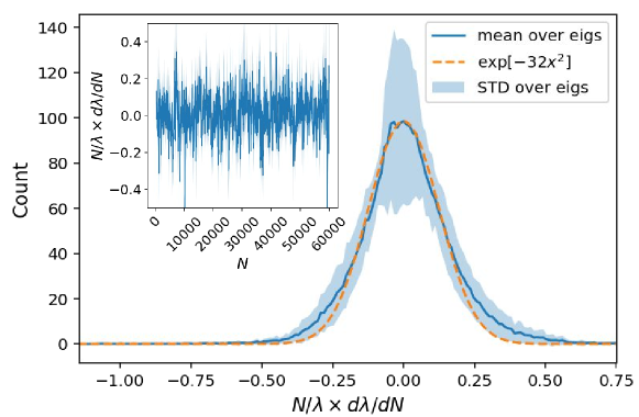
Therefore is also a Gaussian with mean zero and the above variance and we can write . Fig. 3 shows the fluctuations of eigenvalues of for MNIST, where the input is broken into windows convolved over the images (i.e. input for a convolutional layer). is 25 dimensional. When scaled by our prediction of the behavior (20) of the fluctuations, the distribution of the fluctuations of all 25 eigenvalues collapse to a single Gaussian with small error bars, confirming our prediction.

4.2 Solving the weight distribution
Putting all the above together, the weight SGD equations become
| (21) |
where , is a random Gaussian noise with correlation function . Note that this is a stochastic, “Langevin equation” [9]. While there are no solutions to it, we can find the probability distribution for different solutions using the corresponding “Fokker-Planck equation” [16]. We do so by first moving the weights to the right hand side. From the separation of time scales, when in (21) has not fully converged, in the () must be farther from convergence than and must be still fairly random. Thus rows of are uncorrelated, resulting in its transpose being approximately proportional to its pseudo-inverse and so with . As a result, is a projection matrix onto class . Using SVD, we can define a right-pseudo-inverse such that . Define the “class-restricted weights,” . It follows that
| (22) |
which satisfy . Multiplying both sides of (21) by , we get
| (23) |
Since for , we can write111111 Also, note that because of the on the r.h.s. of (21) dimensions that do not get mapped through also do not appear in the SGD equations.
| (24) | ||||
| (25) |
where the “right logarithm,” is formally defined using the pseudo-inverse for the largest non-degenerate submatrix such that121212 Note that is a dimensional matrix, but the its largest non-degenerate submatrix is one dimensional, because of the projection via . . This suggests that (21) could be solved for the class-restricted weights separately, and that for each class we have a stochastic equation given by
| (26) |
This is a Langevin equation with a multivariate noise distributed according to whose magnitude decreases with increasing . The corresponding Fokker-Planck equation has solution (for simplicity )
| (27) |
which is a multivariate Gaussian distribution with spread proportional to the class density matrix. It spreads along directions of eigenvectors of , spreading wider along eigenvectors with larger eigenvalues. This means that for each class, just as in PCA, there are a subset of weights which are likely to be along principal components (PC) of . Since for any orthogonal , we are free to choose the basis of the output of the weights for each layer (i.e. the choice of basis is part of the design of the network architecture). We will therefore choose distinct rows of to be dedicated to each class, trivially satisfying . Then, for each class the most likely outcomes of SGD will be that rows of are PC of . If a PC of one class is highly correlated with a PC of another class, we can keep one of them. The biases canceled in (13) and so in the late stages of training they don’t seem to play a significant role. We may choose . Thus, we can construct pretrained neural networks with weights found using the class-based PCA described here and with biases set to zero. We will call such a network a “Density Matrix Network” (DMN).

4.3 Time Complexity
Training with SGD using mini-batches of data requires calculating the gradients (4), which require matrix product of the weights of layers. Thus the complexity of SGD is
| (28) |
If we replace the lowest layer by a DMN, we remove the factor, but get an additional term for computing the DMN and another for propagating the data through the DMN. Constructing the DMN requires PCA of all , or equivalently SVD of , which has complexity (assuming ). Propagating the input through the DMN is . Thus the complexity of replacing a layer with DMN and training the rest of the network via SGD is
| (29) |
Thus, if and using DMN will certainly result in a reduction in the time complexity of training. In particular, in very deep networks it is more likely to have and thus using DMN can boost the training quite significantly.
5 Simulation and discussion
Training deep neural networks (DNN) requires large amounts of training data and is very computationally expensive. Part of the reason for this is a lack a good mathematical understanding of solutions a DNN converges into. We have shown that it can be possible to derive optimal weights for low-lying layers of a DNN directly from data using a class-based PCA. This relied deeply on a “separation of time scales” which occurs in the highest performing setups for DNNs. We found that when the activation function is similar to ReLU (unbounded from above and asymptotically linear) and the weights are initialized with a high enough variance (allowing the weights to acquire singular values larger than one) lower layers (closer to input) evolve much faster than layers above them. This effectively decouples the SGD dynamics of lower layer from layers above and so SGD will be able to find optimal weights layer-by-layer, starting from closest to the input data. The solutions found by SGD in these cases will be a class-based PCA.
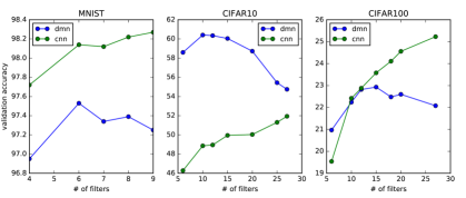
Based on this finding, we can construct pretrained layers using class-based PCA for the weights and setting biases to zero. We will call such a pretrained layer a “Density Matrix Network” (DMN). The class-based PCA consists of calculating the eigenvectors of the covariance matrix of input for each class and keeping the eigenvectors with the largest eigenvalues. The number of eigenvectors to keep depends on how much of the variance of the input data we wish to keep. Additionally, converges very quickly and using only a fraction of the training data used for SGD will still yield DMN performance comparable to SGD in many datasets. We have implemented DMN and tested it on three image data sets. The tested DMNs perform on par, or far superior to conventional networks with the same architecture. DMN is within one percent of the performance of a convolutional layers (ConvNet) on MNIST, and significantly superior to ConvNets on CIFAR10. A single layer DMN also performs much better than a similar ConvNet on CIFAR100, and a two layer DMN is equally good as a 2 layer ConvNet. The results are summarized in Fig. 4. Most of our tested DMNs were trained using a fraction (between 20-70%) of the training data used for the ConvNet.
Note that in these tests DMNs are constructed as convolutional layers131313This is related to the Karhunen-loeve transform of images, where one breaks an image down into blocks and PCA is performed on the block images. . We only have to note that overlapping receptive fields will result in spurious PCs and we need to disentangle the outputs to get rid of them. One simple way to do so is to use a maxpooling layer right after a DMN. We return to this below. The architectures we used for our experiments consist of one or two convolutional layers with ReLU activation functions, each followed by a maxpooling layer and ending with a classification layer with softmax activation function. We run the experiments once with DMNs for the convolutional layers and once with regular ConvNet (More experiments with hybrids of DMN and ConvNet, as well Batch Normalization [15] are presented in the SI).
The supervised PCA, which emerged from SGD, may be related to the “information bottleneck” [30], which we will investigate in the future.
References
- [1] M. Abadi et al. TensorFlow: Large-scale machine learning on heterogeneous systems, 2015. Software available from tensorflow.org.
- [2] M. Abramowitz, I. A. Stegun, and R. H. Romer. Handbook of mathematical functions with formulas, graphs, and mathematical tables, 1988.
- [3] D. J. Amit, H. Gutfreund, and H. Sompolinsky. Spin-glass models of neural networks. Physical Review A, 32(2):1007, 1985.
- [4] E. Barkai, D. Hansel, and I. Kanter. Statistical mechanics of a multilayered neural network. Physical review letters, 65(18):2312, 1990.
- [5] Y. Bengio. Learning deep architectures for ai. Foundations and trends® in Machine Learning, 2(1):1–127, 2009.
- [6] Y. Bengio, P. Simard, and P. Frasconi. Learning long-term dependencies with gradient descent is difficult. IEEE transactions on neural networks, 5(2):157–166, 1994.
- [7] T.-H. Chan, K. Jia, S. Gao, J. Lu, Z. Zeng, and Y. Ma. Pcanet: A simple deep learning baseline for image classification? IEEE Transactions on Image Processing, 24(12):5017–5032, 2015.
- [8] F. Chollet. Keras. https://github.com/fchollet/keras, 2015.
- [9] W. T. Coffey and Y. P. Kalmykov. The Langevin equation: with applications to stochastic problems in physics, chemistry and electrical engineering. World Scientific, 2004.
- [10] V. A. Epanechnikov. Non-parametric estimation of a multivariate probability density. Theory of Probability & Its Applications, 14(1):153–158, 1969.
- [11] E. Gardner. The space of interactions in neural network models. Journal of physics A: Mathematical and general, 21(1):257, 1988.
- [12] X. Glorot and Y. Bengio. Understanding the difficulty of training deep feedforward neural networks. In Proceedings of the Thirteenth International Conference on Artificial Intelligence and Statistics, pages 249–256, 2010.
- [13] I. Goodfellow, Y. Bengio, and A. Courville. Deep learning. 2015, 2016.
- [14] K. He, X. Zhang, S. Ren, and J. Sun. Delving deep into rectifiers: Surpassing human-level performance on imagenet classification. In Proceedings of the IEEE international conference on computer vision, pages 1026–1034, 2015.
- [15] S. Ioffe and C. Szegedy. Batch normalization: Accelerating deep network training by reducing internal covariate shift. In International Conference on Machine Learning, pages 448–456, 2015.
- [16] L. P. Kadanoff. Statistical physics: statics, dynamics and renormalization. World Scientific Publishing Company, 2000.
- [17] S. Kirkpatrick, C. D. Gelatt Jr, and M. P. Vecchi. Optimization by simulated annealing. In Spin Glass Theory and Beyond: An Introduction to the Replica Method and Its Applications, pages 339–348. World Scientific, 1987.
- [18] A. Krizhevsky. Learning multiple layers of features from tiny images. 2009.
- [19] A. Krizhevsky, I. Sutskever, and G. E. Hinton. Imagenet classification with deep convolutional neural networks. In Advances in neural information processing systems, pages 1097–1105, 2012.
- [20] Y. LeCun and Y. Bengio. Convolutional networks for images, speech, and time series. The handbook of brain theory and neural networks, 3361(10):1995, 1995.
- [21] Y. LeCun, Y. Bengio, and G. Hinton. Deep learning. Nature, 521(7553):436–444, 2015.
- [22] Y. LeCun and C. Cortes. MNIST handwritten digit database. 2010.
- [23] M. Loève. Graduate texts in mathematics. Probability Theory I,, pages 159–160, 1977.
- [24] A. L. Maas, A. Y. Hannun, and A. Y. Ng. Rectifier nonlinearities improve neural network acoustic models. In Proc. ICML, volume 30, 2013.
- [25] A. Mahendran and A. Vedaldi. Visualizing deep convolutional neural networks using natural pre-images. International Journal of Computer Vision, 120(3):233–255, 2016.
- [26] J. Schmidhuber. Learning complex, extended sequences using the principle of history compression. Neural Computation, 4(2):234–242, 1992.
- [27] R. Shwartz-Ziv and N. Tishby. Opening the black box of deep neural networks via information. arXiv preprint arXiv:1703.00810, 2017.
- [28] K. Simonyan and A. Zisserman. Very deep convolutional networks for large-scale image recognition. arXiv preprint arXiv:1409.1556, 2014.
- [29] M. Telgarsky. Benefits of depth in neural networks. arXiv preprint arXiv:1602.04485, 2016.
- [30] N. Tishby, F. C. Pereira, and W. Bialek. The information bottleneck method. arXiv preprint physics/0004057, 2000.
- [31] M. Wand and M. Jones. Kernel smoothing london, 1995.
- [32] J. Yosinski, J. Clune, Y. Bengio, and H. Lipson. How transferable are features in deep neural networks? In Advances in neural information processing systems, pages 3320–3328, 2014.
Supplemental Information: Separation of time scales and direct computation of weights in deep neural networks
Nima Dehmamy∗,
Neda Rohani†
Aggelos Katsaggelos†
CCNR, Northeastern University, Boston 02115 MA, USA
IVPL, Northwestern University, Evanston, 60208 IL, USA
SI 6 Smoothing of energy landscape
SI 7 Singular Values of weights during SGD
To quantify the effect of , we must examine its singular values and find out how they evolve with training steps, i.e. increasing . Define . At step zero, weights and biases of all layers are random and so we can assume that half of the entries of will be zero, the other half one. Thus, in half of the rows of will be replaced by zeros. Consider the symmetric positive semi-definite matrix . The eigenvalues of are squares of singular values (SV) of . The are generally initialized randomly with zero mean. As columns of are uncorrelated at the start, will be approximately diagonal and all diagonal entries will be similar because
| (30) |
where is the variance of the weights over the input dimension and the is because of eliminating half of the rows. The variance of all rows is chosen to be the same initially. Eq. (30) implies that most eigenvalues of are initially close to . Now consider whose eigenvalues are squares of SV of . Using (30) we can progressively simplify and get
| (31) |
where is the identity matrix. Experiments have shown [14] that with ReLU, the Glorot initialization [12] (a variant of the Xavier method) which sets yields better performance than other commonly used initialization methods. Glorot initialization was designed specifically to set the maximum SV of all around one to avoid explosion of gradients, while choosing a smaller initialization makes the gradients too small and leads to worse results. However, this initialization does not guarantee that the maximum SV will remain below one. In fact, we argue that the reason this choice works better than a smaller initialization is precisely because the SV become larger than one early in SGD.
SI 7.1 Magnitude of
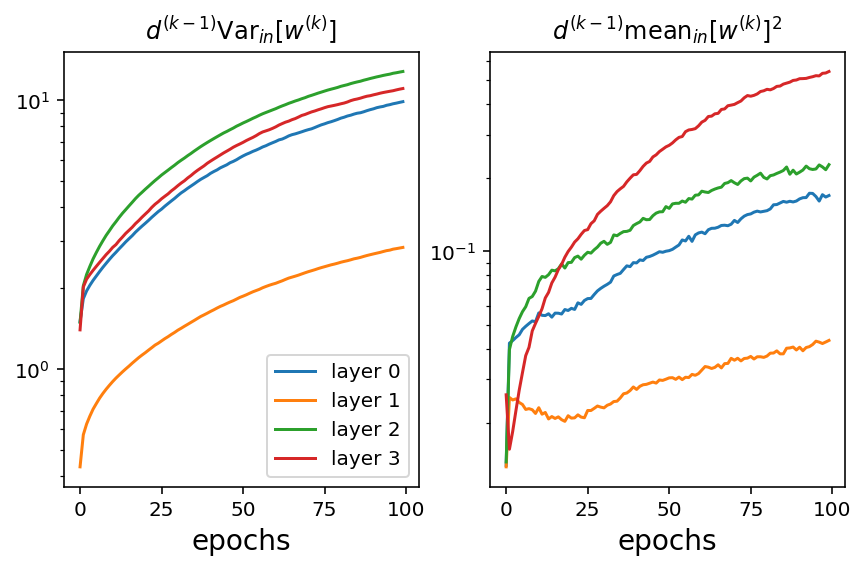
One may argue that contains the product of the weights of the first layers and therefore the gradients of for all are of the same magnitude. But it is easy to see that cannot remain . To see this, we examine the change in after processing a minibatch during SGD. Using (3)–(4), we have
| (32) | ||||
| (33) | ||||
| (34) |
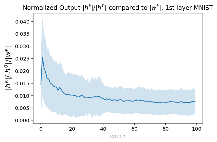
Fig. 3 shows the magnitude of divided by the magnitude of the weights and the input in a network consisting of a ConvNet with kernels followed by a dense classification layer being trained on MNIST. As we see the maginitude of the output does not become comparable to which itself is larger than and is, in fact, orders of magnitude smaller.
SI 8 Distribution of eigenvalues of a random matrix with positive entries
Recall that the characteristic equation has the form , so the sum of the eigenvalues is the trace , which for a random matrix is also the mean of each row. Wigner’s semicircle law [2] states that the eigenvalues are distributed symmetrically around zero with radius . Since the trace is invariant under unitary transformations, it is the sum of the eigenvalues and as the semi-circle eigenvalues are symmetric around zero they all cancel, leaving only the highest eigenvalue. Thus the largest eigenvalue is the trace.
SI 9 Relation of added data and changes in the density matrix
In (16) is the guessed input based on the previous inputs and it can be expressed as a linear combination141414Note, may be overcomplete and not be linearly independent, but only needs to map onto a linearly independent subset of them. of previous inputs which belonged to the same class as
and consequently . The last input , on the other hand, contains new information and it cannot be an orthogonal transformation on them. Thus we write where , but is not orthogonal. Since we have freedom in choosing , we can choose and so we have
| (35) | ||||
| (36) | ||||
| (37) |
Thus
| (38) |
SI 9.1 Dynamics of Relaxation of the Density Matrix
In the relaxation phase fluctuates mostly due to statistical fluctuations in the data. As every input is an independent drawing from the dataset, is the sum of observations of a random variable . Thus, as it contains samples. Using the Bienaymé formula [23] and the fact that is quadratic in , we have . Since mean and variance of the input do not diverge, Central Limit Theorem implies that will have a multivariate Gaussian distribution. Using Gaussianity we can directly calculate
| (39) | ||||
| (40) |
Therefore is also a Gaussian with mean zero and the above variance and we can write . Fig. 4 shows the fluctuations of eigenvalues of for MNIST, where the input is broken into windows convolved over the images (i.e. input for a convolutional layer). is 25 dimensional. When scaled by our prediction of the behavior (20) of the fluctuations, the distribution of the fluctuations of all 25 eigenvalues collapse to a single Gaussian with small error bars, confirming our prediction.
SI 10 Convergence of layers
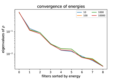
Fig. 5 shows empirical evidence that lower layers descend faster compared to higher layers.

SI 11 Lessons from Linear Regression
To anticipate our results about Stochastic Gradient Descent (SGD) in neural networks, let us illustrate what we would find if we were to solve linear regression using SGD.
Suppose we have a set of input vectors , with -dimensional , and -dimensional labels . We wish to find the linear transformation which minimizes the mean squared error (MSE)
| (41) |
The solution is where . Of course, in nonlinear settings, such neural networks, this solution cannot be calculated and we need to resort to methods such as SGD. During SGD, a new batch of data and are added at each step and the estimate for is corrected based on the gradient of .
| (42) | ||||
| (43) |
Note that is a matrix and all products are matrix multiplication. is and is similar to a covariance matrix, only without subtracting the mean. We will refer to as the “density matrix”. We are seeking the effect of adding the th data point. Thus is evaluated using the previous data points. The optimal value for at is where contain only the initial data points and not , unlike in (43). We will assume the label dimension is much smaller than the input dimension, i.e. . This means that the rank of can be at most and that a right-pseudo-inverse yields where is a -dimensional projection onto a -dimensional subspace. Given labels , we may use the pseudo-inverse to find a “best guess” for what the input might have been
| (44) |
although and so are not unique, holds because is the exact solution using the data points. But because isn’t optimazed using , . Using (44) and defining , we have
| (45) | ||||
| (46) | ||||
| (47) |
thus eliminating from (43) we get
| (48) | ||||
| (49) |
Notice that is found using the , estimated using data points. Therefore, unlike (44), we have
To better understand what (49) means we will write out explicitly. One explicit form for is . Thus
Writing the input and label as a linear combination of the previous data, we get
| (50) | ||||
| (51) |
where is an vector and thus is a rank 1 projection. Since are iid, the transformation will uniformly sample previous and so . Writing and using yields
| (52) | ||||
| (53) | ||||
| (54) |
Thus we have
| (55) |
Finally, we have found that SGD (49) is in fact relating changes in weights to changes in data covariance (55)
| (56) |
This equation can be solved by defining a “right logarithm” defined such that
Thus, we find an equation similar what we found for the relaxation phase of a classification problem, except that it does not contain the projection on label classes . This is, of course, because there are no label classes in a regression problem. But this also points that the linearization we used to solve the relaxation phase is implicitly assuming that the layer is stuck inside one local minimum and that the problem reduces to a set of convex optimization problems for the label classes, which explains why we were able to solve it. The confinement to a single local minimum in the relaxation phase for the lowest layer makes sense because in this phase statistical fluctuations are not large enough to allow the layer to tunnel to a different minimum.
SI 12 Simulations
SI 13 Creating trained network layers
Our results show that in many problems, the optimal weights in the first few layers can be found using supervised PCA. What contrasts this from normal PCA is that each class has a different covariance (“density”) matrix and the principal components (PC) may not completely overlap for different classes. As described above, the supervised PCA consists of calculating the eigenvectors of the covariance matrix of input for each class and keeping the largest eigenvalue/ eigenvector pairs. The number of eigenvectors to keep depends on how much of the variance of the input data we wish to keep. Additionally, the converges very quickly and using only a fraction of the training data will still yield performance comparable to using all of the training data in many datasets. We have experimented with different values for fraction of training data and amount variance of data used for choosing the eigenvectors, as summarized in table 2 for MNIST and CIFAR10 datasets.
We will refer to the construction described above as the Density Matrix Network (DMN). Regular PCA has been used for creating trained layers in [7], but that architecture, called PCANet, involves extra steps, which we will not have in DMN. Even DMNs using regular PCA perform well in the first layer, but worsen in performance in higher levels (see below). But DMNs using the class-based, supervised PCA perform within one percent of a convolutional layers (ConvNet) on MNIST [22], and significantly superior to ConvNets on CIFAR10 [18]. A single layer DMN also performs much better than a similar ConvNet on CIFAR100 [18], and a two layer DMN is equally good as a 2 layer ConvNet. The results are summarized in Fig. 4. Notice that it takes much less time and computation to calculate weights in a DMN as repeated backpropagation is not needed and a fraction of the training data may be sufficient.
A DMN can also be constructed as a convolutional layer. This is related to the Karhunen-loeve transform of images, where one breaks an image down into blocks and PCA is performed on the block images. We only have to note that overlapping receptive fields will result in spurious PCs and we need to disentangle the outputs to get rid of them. One simple way to do so is to use a maxpooling layer right after a DMN. We return to this below. The architectures we used for our experiments consist of one or two convolutional layers with ReLU activation functions, each followed by a maxpooling layer and ending with a classification layer with softmax activation function. We run the experiments once with DMNs for the convolutional layers and once with regular ConvNet (More experiments with hybrids of DMN and ConvNet, as well Batch Normalization [15] are shown in SM).
SI 13.1 Disentangling the Weights using Pooling
For images, convolutional layers work because they exploit the translational symmetry, or the fact that features can be anywhere in the image. However, when doing PCA, we rely on the input data to have correlations only due to features intrinsic to the data. Overlapping domains in convolution introduce spurious correlations, and hence spurious PCs, which become the most prominent PCs in PCA. This dramatically reduces the performance of PCA, as actual features intrinsic to the data become much less significant than the spurious ones. Thus, to correctly employ our result and use PCA to extract higher level features, the spurious correlations (“entanglements”) should be removed. While finding the optimal way to do so may be elaborate, a simple solution is to use maxpooling. This will only keep one out of a few overlapping outputs and greatly reduce the entanglement. therefore, we use maxpooling after every layer of DMN in all our simulations.
SI 14 Simple PCA layers
Even without the supervised PCA, regular PCA can ield fairly well performing first layers. In subsequent layrs, however, regular PCA performs poorly, mainly becuase the selected filters are not conditioned on the labels and thus may emphasize features that do not help with the classification, but rather are prominent in the data.
To train a DMN, we simply need to find the eigenvectors of the density matrices . We will test a naive version of DMN, assuming that is is roughly independent of in the first and second layer. This is equivalent to assuming that the low-level features contribute with similar proportions to all label classes. This way, training a DMN is the same as doing PCA on the full . When the the dataset is randomly sampled, converges very quickly (Fig. 7 SM). Thus, using only a fraction of the data can give us a very good estimate for training a DMN, which can reduce the training time significantly. Since a DMN is pretrained, the removal of one layer from backpropagation may also result in a boost in training time, especially in very deep networks.
To examine the applicability of DMN layers in neural network architectures for image classification, we performed a number of tests on three image datasets: MNIST [22], CIFAR10 [18] and CIFAR100 [18]. We simulate different scenarios and define different architectures with one or two DMNs/convolutional (Conv.) layers and compare their classification accuracies. We use Keras [8] with Tensorflow [1] back-end for all implementations. To study the effect of DMNs and Conv. layers in the classification task, our architectures will include only one dense layer, which is the classification layer followed by a softmax activation layer. Aside form this dense layer, the basic building block of our architectures consists of a convolutional layer, ReLU activation layer and a maxpooling layer (for disentanglement). We use either one or two conv. layers. Then we replace these conv. layers with DMNs and measure how the performance changes (see Fig. 9 in SM for a sketch of the architectures). We will denote a DMN layer with 15 filters by “d15”, a Conv. layer with 15 filters as “c15”, max pooling with pool size of 2 as “m”, and dense layer with 10 nodes as “de10”. For DMN and Conv. layers, the kernel size has been fixed to 3. In some experiments, we have added a batch normalization layer and we denote such layer by “BN”.
In MNIST and CIFAR10 datasets we have 10 classes. Therefore in the baseline model (i.e. with no conv. layers), the network consists of a single dense layer with perceptrons and softmax activation function. For CIFAR100 model, the dense layer has perceptrons. Next, we make the network deeper by adding one or two DMN or Conv. layers. We test the effect of the number of filters on the performance of DMN and ConvNet.
For the first set of the experiments, which have a single DMN or Conv. layer, With one DMN, we observe that more filters does not necessarily yield better accuracy (maximum possible filters ) (Fig. 6). However, for a network with one Conv. layer, the classification accuracy increases by the number of layers. The key point to note here is that, DMN with maximum possible filters becomes a linear layer, whereas having less filters means we are only keeping the most prominent PCs, discarding less prominent features. for every dataset, there exists an optimal number of filters that leads to best performance of a DMN (e.g. 6 for MNIST, 12 for CIFAR10, and 15 for CIFAR100). The results of this experiment are shown in Fig. 6. Comparing the blue “DMN” line with green “Conv” line, we observe that the performance of 1 DMN layer is comparable with 1 Conv. layer. For CIFAR10 dataset, we see that one DMN layer outperforms one Conv. layer. In conclusion, we have shown that we can replace a Conv. layer with a DMN layer without degrading the classification accuracy.
In the second set of experiments we use two-layer network with different settings: 1. two DMNs, 2. one DMN and one Conv. layer and 3. two Conv. layers. Fig. 10 reports the results of two layer networks applied to three datasets. For MNIST dataset, we can observe that adding the second DMN layer increases the classification accuracy slightly. The performance of networks with one DMN and one Conv. layer is very close to two Conv. layer networks. For CIFAR10 dataset, without using BN layer, the networks with two DMN layers have lower classification accuracy compared to one DMN layer network. However, when we add a BN layer, the classification accuracy increases slightly. The best performance achieves by networks with one DMN and one Conv. layer and the worst performance is obtained by two Conv. layer networks. For CIFAR100 dataset, adding the second DMN layer results in higher accuracy as can be observed from Fig. 10. The highest accuracy is achieved by a network composed of one DMN layer and one Conv. layer. The first layer provides a better base filters and the input data is transformed to a more meaningful feature space. Adding a Conv. layer, back-propagation and training the network increases the classification accuracy (The classification accuracies of different architectures are summarized in tables 3, 4, 5 in SM). Here, we plot the effect of number of filters used in DMN layer in one layer DMN network on the classification accuracy and compare it with one Conv. layer network with the same number of filters.
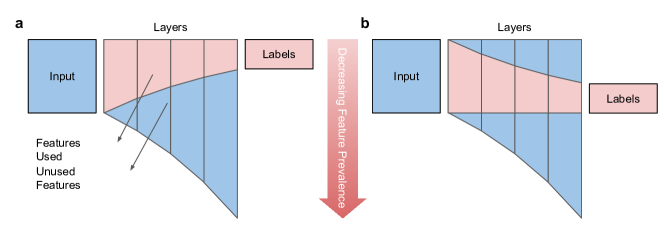
SI 15 A type of information bottleneck
Aside from the supervised PCA, we have also shown that in cases where the classes use low-level features in a similar fashion (e.g. the MNIST dataset), one can achieve good performance using even an unsupervised PCA, agnostic to the class of the output. In cases such as CIFAR10, however, the labels are very restrictive and each class uses low-level features in different proportions compared to the total amount features present in the data. Moreover, the labels may pertain to rare and specific features, not necessarily the most common features in the dataset. In these cases, simple PCA does not perform well beyond the first layer and the supervised, PCA mentioned, needs to be used to fine-tune the weights to features relevant to each class. We have confirmed this in our simulations, shown in Figs. 6 and 10. We work on three datasets: MNIST, CIFAR10 and CIFAR100. We use a naive DMN, i.e. agnostic to labels and trained using basic PCA. In all three datasets, one layer of DMN performs at least as good as a similar convolutional layer. We also find that, while adding a second layer to MNIST and CIFAR100 significantly improves classification, it actually worsens the classification in CIFAR10, supporting our hypothesis that naive PCA will not help beyond first layer.
SI 16 Other simulations and test
| MNIST | |||||
|---|---|---|---|---|---|
| Arch. | Input | Var. | Cutoff | Val. Acc. | ConvNet Acc. |
| d4 | 0.5 | 0.85 | 0.9 | 96.81 | 97.47 |
| d6 | 0.3 | 0.95 | 0.9 | 97.78 | 98.12 |
| d16 | 0.3 | 0.99 | 0.9 | 97.28 | 98.37 |
| d4, d15 | 0.5 | 0.85 | 0.9 | 97.84 | 98.63 |
| d6, d93 | 0.3 | 0.95 | 0.9 | 98.5 | 98.86 |
| CIFAR10 | |||||
|---|---|---|---|---|---|
| Arch. | Input | Var. | Cutoff | Val. Acc. | ConvNet Acc. |
| d10 | 0.7 | 0.99 | 0.9 | 49.92 | 48.61 |
| d10, d11 | 0.7 | 0.99 | 0.9 | 49.94 | 46.88 |
| d22 | 0.7 | 0.999 | 0.9 | 56.2 | 49.94 |
| d22, d41 | 0.2 | 0.995 | 0.9 | 59.64 | 51.96 |
| d22, d41 | 0.7 | 0.995 | 0.9 | 59.48 | 51.96 |
| d22, d87 | 0.7 | 0.997 | 0.9 | 62.15 | 52.66 |
| d22, d305 | 0.7 | 0.999 | 0.9 | 63.71 | 52.13 |
| CIFAR100 | |||||
|---|---|---|---|---|---|
| Arch. | Input | Var. | Cutoff | Val. Acc. | ConvNet Acc. |
| d79 | 1 | 0.999 | 0.9 | 30.93 | 26.14 |
| d79, d545 | 1 | 0.995 | 0.9 | 38.38 | 38.38 |
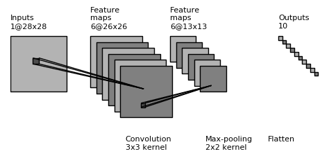
(a)
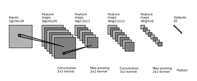
(b)

| arch. | training acc. | validation acc. |
|---|---|---|
| de10 | 93.51 | 92.90 |
| d6, m, de10 | 99.29 | 97.53 |
| c9, m, de10 | 99.35 | 98.27 |
| d9, m, d40, m, de10 | 98.78 | 98.10 |
| d6, m, d54, m, BN, de10 | 99.90 | 98.39 |
| d9, m, BN, c81, m, de10 | 99.98 | 99.07 |
| c6, m, c40, m, de10 | 99.64 | 99.06 |
| arch. | training acc. | validation acc. |
|---|---|---|
| de10 | 43.11 | 40.06 |
| d10, m, de10 | 73.21 | 60.41 |
| c27, m, de10 | 62.69 | 51.94 |
| d15, m, d108, m, de10 | 66.11 | 55.36 |
| d20, m, d180, m, BN, de10 | 66.02 | 63.66 |
| d15, m, c80, m, de10 | 79.21 | 68.03 |
| d27, m, c108, m, BN, de10 | 81.18 | 71.19 |
| c10, m , c80, m, de10 | 58.48 | 50.10 |
| c32, m, c32, m, de10 | 58.64 | 51.84 |
| arch. | training acc. | validation acc. |
|---|---|---|
| de100 | 23.68 | 15.96 |
| d15, m, de100 | 37.48 | 22.93 |
| d18, m, BN, de100 | 51.07 | 30.30 |
| c27, m, de100 | 41.31 | 25.23 |
| d15, m, d50, m, de100 | 51.57 | 25.93 |
| d18, m, d108, m, BN, de100 | 53.58 | 34.76 |
| d15, m, c108, m, de100 | 65.06 | 36.56 |
| d27, m, BN, c108, m, de100 | 63.57 | 41.03 |
| c32, m, c32, m, de100 | 33.03 | 23.07 |
| c27, m, c108, m, de100 | 36.95 | 23.97 |