Quadratic Feynman Loop Integrands From Massless Scattering Equations

Abstract

Recently the Cachazo-He-Yuan (CHY) approach has been extended to loop level, but the resulting loop integrand has propagators that are linear in the loop momentum unlike Feynman’s. In this note we present a new technique that directly produces quadratic propagators identical to Feynman’s from the CHY approach. This paper focuses on $\Phi^{3}$ theory but extensions to others theories are briefly discussed. In addition, our proposal has an interesting geometric meaning, we can interpret this new formula as a unitary cut on a higher genus Riemann surface.

1 Introduction

Since the remarkable work of Witten Witten:2003nn on the ${\cal N}=4$ super Yang–Mills theory, the on-shell methods for the computation of scattering amplitudes have been deeply studied during the last years. In particular, the Cachazo–He–Yuan (CHY) approach Cachazo:2013gna ; Cachazo:2013hca ; Cachazo:2013iaa ; Cachazo:2013iea , which is applicable in arbitrary dimension, is an outstanding method because it can be applied for a large family of interesting theories including scalars, gauge bosons, gravitons and mixing interactions among them Cachazo:2014xea ; Cachazo:2014nsa ; Cachazo:2016njl . The original proposal is to write the tree-level S-matrix in terms of a contour integral localized over solutions of the so-called scattering equations Cachazo:2013gna on the moduli space of $n$-punctured Riemann spheres. Other approaches that use the same moduli space include the Witten–RSV Witten:2003nn ; Roiban:2004yf , Cachazo–Geyer Cachazo:2012da , and Cachazo–Skinner Cachazo:2012kg constructions, but are special to four dimensions.

The CHY formalism has already been verified to reproduce well-known results, such as the soft limits of various theories Cachazo:2013hca , the Kawai–Lewellen–Tye relations Kawai:1985xq between gauge and gravity amplitudes Cachazo:2013gna , as well as the correct Britto–Cachazo–Feng–Witten Britto:2005fq recursion relations in Yang–Mills and bi-adjoint $\Phi^{3}$ theories Dolan:2013isa .

Nevertheless, a direct evaluation of the CHY-integrals for higher order poles is not a simple task. So, many methods have been developed during the last year to deal with them. These attempts include the study of solutions at particular kinematics and/or dimensions Cachazo:2013iea ; Kalousios:2013eca ; Lam:2014tga ; Cachazo:2013iaa ; Cachazo:2016sdc ; He:2016vfi ; Cachazo:2015nwa ; Cachazo:2016ror , encoding the solutions to the scattering equations in terms of linear transformations Kalousios:2015fya ; Dolan:2014ega ; Huang:2015yka ; Cardona:2015ouc ; Cardona:2015eba ; Dolan:2015iln ; Sogaard:2015dba ; Bosma:2016ttj ; Zlotnikov:2016wtk ; Mafra:2016ltu , or the formulation of integration rules in terms of the polar structures Baadsgaard:2015ifa ; Baadsgaard:2015voa ; Huang:2016zzb ; Cardona:2016gon . In particular, the author in Gomez:2016bmv gave an independent proposal by generalizing the double-cover formulation, the so-called $\Lambda$-algorithm, which we are going to use in this paper.

The CHY formalism has been generalized to loop level. Using the ambitwistor and pure spinor ambitwistor string Mason:2013sva ; Berkovits:2013xba ; Gomez:2013wza , a proposal was made in Geyer:2015bja ; Geyer:2015jch ; Adamo:2015hoa . Parallelly, in Cachazo:2015aol ; He:2015yua ; Baadsgaard:2015hia , another prescription was developed by performing a forward limit on the scattering equations for massive particles formulated previously in Naculich:2014naa ; Dolan:2013isa . On the other hand, the author et al, following the ideas presented in Gomez:2016bmv , obtained an alternative formulation at one-loop by embedding the torus in a $\mathbb{CP}^{2}$ through an elliptic curve Cardona:2016bpi and used it to reproduce the $\Phi^{3}$ theory at one loop Cardona:2016wcr . Recently, in Chen:2016fgi ; Chen:2017edo a differential operators on the moduli space were created to compute CHY-integrals at one-loop. In addition, extensions at two-loop are being studied and some important results have been found in Geyer:2016wjx ; Feng:2016nrf ; Gomez:2016cqb .

However, all results obtained at loop level from the CHY approach do not match in an exact way with the Feynman diagrams. In order to establish an equivalence among the CHY approach and the Feynman integrads at loop level, it is needed to use the partial fraction identity (${\rm p.f}$)

$${1\over\prod_{i=1}^{n}D_{i}}=\sum_{i=1}^{n}{1\over D_{i}\prod_{j\neq i}(D_{j}-D_{i})}\,$$

and after shifting (${\rm S}$) the internal loop momentum. This is not a trivial process and its real matching is still analized Huang:2015cwh ; Baadsgaard:2015twa ; Feng:2016msc . For example, let us consider the symmetrized $\Phi^{3}$ Feynman diagram in figure 1.

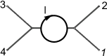
Figure 1: $\Phi^{3}$ symmetrized Feynman diagram.

The expression for this amplitude is given by

$${\cal A}^{\rm FEY}=\int d^{D}\ell\,\,{\cal I}^{\rm FEY}=\int\frac{d^{D}\ell}{s_{12}s_{34}}\left[\frac{1}{\ell^{2}\,(\ell+k_{1}+k_{2})^{2}}+\frac{1}{\ell^{2}\,(\ell-k_{1}-k_{2})^{2}}\right].$$

Now, from the CHY approach at one-loop Cardona:2016bpi ; Cardona:2016wcr , the result for the same process is

$${\cal A}^{\rm CHY}=\int d^{D}\ell\,\,{\cal I}^{\rm CHY}=2\int\frac{d^{D}\ell}{s_{12}s_{34}}\left[\frac{1}{\ell^{2}\,\left[(\ell+k_{1}+k_{2})^{2}-\ell^{2}\right]}+\frac{1}{\ell^{2}\left[(\ell-k_{1}-k_{2})^{2}-\ell^{2}\right]}\right],$$

which is referred to as the Q-cut representation Baadsgaard:2015twa . In order to obtain an equivalence at the integrand level, we apply the partial fraction identity in ${\cal A}^{\rm FEY}$, so it becomes

$${\cal A}^{\rm FEY}\Big{|}_{\rm p.f}= \int\frac{d^{D}\ell}{s_{12}s_{34}}\left[\frac{1}{\ell^{2}\,\left[(\ell+k_{1}+k_{2})^{2}-\ell^{2}\right]}+\frac{1}{(\ell+k_{1}+k_{2})^{2}\,\left[\ell^{2}-(\ell+k_{1}+k_{2})^{2}\right]}\right.$$

$$\qquad\qquad\left.+\frac{1}{\ell^{2}\left[(\ell-k_{1}-k_{2})^{2}-\ell^{2}\right]}+\frac{1}{(\ell-k_{1}-k_{2})^{2}\left[\ell^{2}-(\ell-k_{1}-k_{2})^{2}\right]}\right].$$

At last, by performing the shift transformations, $\ell^{\prime}=\ell+k_{1}+k_{2}$ and $\ell^{\prime}=\ell-k_{1}-k_{2}$, in the second and fourth term on ${\cal A}^{\rm FEY}\Big{|}_{\rm p.f}$, respectively, it is simple to check how the amplitude ${\cal A}^{\rm FEY}$ becomes ${\cal A}^{\rm CHY}$.

In this work we give, for first time, a proposal which is able to reproduce the physical quadratic Feynman integrand at one-loop from the CHY approach, i.e. it is not necessary to use the partial fraction identity nor shifting the loop momentum. Although in this paper we are just focused to the $\Phi^{3}$ theory, we are working to extend our ideas to other theories and also at two-loop wp . Our formula, which is motived from two-loop prescription given in Gomez:2016cqb , is simple and it includes into itself the results found in Cardona:2016bpi ; Cardona:2016wcr , as it is shown in section 4 and argued in section 5.

One of the main virtues of this new proposal is that the CHY integrals are localized on the original scattering equations given in Cachazo:2013gna ; Cachazo:2013hca ; Cachazo:2013iaa . Let us be more explicit, if we wish to obtain the quadratic Feynman integrand of a scattering of $n$ massless particles at one-loop using this new CHY proposal, then we must solve the scattering equations of $(n+4)$ on-shell particles, i.e.

$$E_{A}=\sum_{B=1\atop B\neq A}^{n+4}\frac{k_{A}\cdot k_{B}}{\sigma_{AB}}=0,\qquad k_{A}^{2}=0,\qquad A=1,\ldots,n+4.$$

This means that all methods developed to compute CHY integrals of massless particles can be used without any restriction, in particular the $\Lambda-$algorithm Gomez:2016bmv , which will be used in section 4.

Finally, one can summarize saying we have found a novel form to write the scattering amplitudes at one-loop from an unitary cut on a Riemann surface of genus two. Schematically our result is represented in figure 2,

 

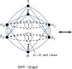
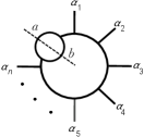
Figure 2: Schematic representation for the new CHY proposal.

where the measure $d\Omega$ is defined as

$$d\Omega: =d^{D}(k_{a_{1}}+k_{b_{1}})\,\delta^{(D)}(k_{a_{1}}+k_{b_{1}}-\ell)\,d^{D}k_{a_{2}}\,d^{D}k_{b_{2}}\,\delta^{(D)}(k_{a_{2}}+k_{a_{1}})\,\,\delta^{(D)}(k_{b_{2}}+k_{b_{1}}).$$

and the Dirac delta functions in $d\Omega$ guarantees the unitary cut. For instance, let us consider the Feynman integrand given in the above example in the amplitude ${\cal A}^{\rm FEY}$, figure 1. So, from this new proposal the CHY integrand represented in figure 3 is able to reproduce the same ${\cal I}^{\rm FEY}$ integrand.

    

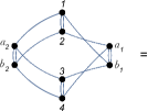
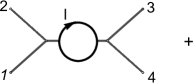
Figure 3: Equality among CHY and Feynman integrands.

This new representation is going to be explained in detail in section 3 and 5.

Outline

This paper is organized in the following way. In section 2 we present a general review of the CHY approach at one-loop for the $\Phi^{3}$ theory. As we emphasize, the equivalence with the Feynman diagrams is obtained after using the partial fraction identity and by shifting the loop momentum. In section 3 we propose a new formula to obtain quadratic Feynman integrands from the CHY approach. Notice that the new CHY-integrand proposed in (13) is totally similar to the one already known given in (4), with the big difference that there are two more particles. In section 4 we give some examples in order to illustrate our new formula proposed in section 3. The computations are presented in detail, so in each example one can see as the old one-loop prescription, given in section 2, contributes to the final answer. To end, in section 5 we present some conclusions and make clear our motivation to propose the formula given in section 3. In addition, a few perspectives are put in context.

Before beginning with the review at one-loop, we define the notation that is going to be used in the paper.

Notation

In order to have a graphical description for the CHY integrands on a Riemann sphere (CHY-graphs), it is convenient to represent the factor ${1\over\sigma_{ab}}$ as a line and the factor $\sigma_{ab}$ as a dashed line that we call the anti-line:

$${1\over\sigma_{ab}}\,\leftrightarrow\,a~{}\overline{~{}~{}~{}~{}~{}~{}~{}~{}~{}~{}~{}~{}~{}}~{}b~{}~{}~{}{\rm(line)},$$ (1)

$$\sigma_{ab}~{}\leftrightarrow\,a\,-\,-\,-\,-\,b~{}~{}~{}{\rm(anti{\rm-}line)}.$$ (2)

Additionally, since we often use the CHY-graphs and the $\Lambda-$algorithm Gomez:2016bmv , it is useful to introduce the color code given in figure 4 for a mnemonic understanding.

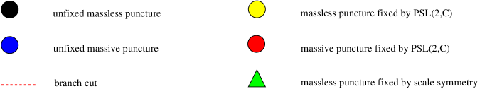
Figure 4: Color code in CHY-graphs.

Finally, we introduce the following notation

$$k_{\{a_{1},\ldots,a_{m}\}}=[a_{1},\ldots,a_{m}]:=\sum_{i=1}^{m}k_{a_{i}},\quad s_{a_{1}\ldots a_{m}}:=k_{\{a_{1},\ldots,a_{m}\}}^{2},\quad k_{a_{1}\ldots a_{m}}:=\sum_{a_{i}<a_{j}}^{m}k_{a_{i}}\cdot k_{a_{j}},$$

$$\sigma_{ij}:=\sigma_{i}-\sigma_{j},\quad(i_{1},i_{2},\ldots,i_{p}):=\sigma_{i_{1}i_{2}}\cdots\sigma_{i_{p-1}i_{p}}\sigma_{i_{p}i_{1}},\quad\omega_{i:j}^{a:b}:=\frac{\sigma_{ab}}{\sigma_{ia}\,\,\sigma_{jb}},$$ (3)

$$B(A,B,C,D):=\frac{1}{k_{A}\cdot k_{C}+\frac{1}{2}k_{A}^{2}}+\frac{1}{k_{A}\cdot k_{D}+\frac{1}{2}k_{A}^{2}},$$

where $A,B,C$ and $D$ are sets, for example $A=\{a_{1},a_{2},\ldots a_{p}\}$, and $k_{A}=k_{\{a_{1},a_{2},\ldots a_{p}\}}$. Note that $\omega_{i:j}^{a:b}$ is the generalization of the $(1,0)-$forms used in Gomez:2016cqb to write the CHY integrands at two-loop.

2 Simple Review of CHY $\Phi^{3}$ Integrand at One-Loop

In this section we present a simple and quick review about CHY integrands at one-loop. This is going to be very useful in order to compare and understand our new results.

As it was shown in Cardona:2016bpi ; Cardona:2016wcr ; Geyer:2015bja ; Geyer:2015jch ; Gomez:2016cqb ; He:2015yua ; Chen:2016fgi , the CHY integrand at one loop of the symmetrized $n$-gon can be written as

$${\bf I}^{\rm n-gon}_{\rm sym} =\frac{1}{(\ell^{+},\ell^{-})^{2}}\left(\omega_{1:2}^{\ell^{+}:\ell^{-}}\,\omega^{\ell^{+}:\ell^{-}}_{2:3}\,\cdots\omega^{\ell^{+}:\ell^{-}}_{n:1}\right)\times\left(\omega^{\ell^{+}:\ell^{-}}_{1:n}\,\omega^{\ell^{+}:\ell^{-}}_{n-1:n-2}\,\cdots\omega^{\ell^{+}:\ell^{-}}_{2:1}\right),$$ (4)

The CHY-graph representation for ${\bf I}^{\rm n-gon}_{\rm sym}$ is given on the right side in figure 5.

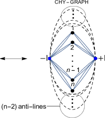
Figure 5: Correspondence between the $\Phi^{3}$ Feynman diagrams ($n$-gon-symmetrized) and the CHY graphs, up to partial fraction identity and $\frac{1}{\ell^{2}}$ factor. $S_{n}$ is the permutation group and $\alpha_{i}:=\alpha(i)$.

By integrating ${\bf I}^{\rm n-gon}_{\rm sym}$ over the moduli space, i.e.

$${\cal I}^{\rm n-gon-CHY}_{\rm sym}:={1\over\ell^{2}}\int d\mu^{\rm 1-loop}\,\,\,I^{\rm n-gon}_{\rm sym},$$ (5)

with

$$d\mu^{\rm 1-loop}:= \frac{1}{{\rm Vol}\,\,({\rm PSL}(2,\mathbb{C}))}\times\frac{d\sigma_{\ell^{+}}}{E^{\rm 1-loop}_{\ell^{+}}}\times\frac{d\sigma_{\ell^{-}}}{E^{\rm 1-loop}_{\ell^{-}}}\times\prod_{a=1}^{n}\frac{d\sigma_{a}}{E^{\rm 1-loop}_{a}},$$

$${}^{\underrightarrow{\,\quad{\rm fixing\,\,PSL}(2,\mathbb{C})\,\quad}}\,\,\,\prod_{i=1}^{n-1}\frac{d\sigma_{i}}{E^{\rm 1-loop}_{i}}\times(\sigma_{\ell^{+}\ell^{-}}\,\sigma_{\ell^{-}n}\,\sigma_{n\ell^{+}})^{2}$$ (6)

and

$$E_{a}^{\rm 1-loop}:=\sum^{n}_{b=1\atop b\neq a}\frac{k_{a}\cdot k_{b}}{\sigma_{ab}}+\frac{k_{a}\cdot\ell^{+}}{\sigma_{a\ell^{+}}}+\frac{k_{a}\cdot\ell^{-}}{\sigma_{a\ell^{-}}},$$ (7)

$$E_{\ell^{\pm}}^{\rm 1-loop}:=\sum^{n}_{b=1}\frac{\ell^{\pm}\cdot k_{b}}{\sigma_{\ell^{\pm}b}},\qquad(\ell^{+})^{\mu}=-(\ell^{-})^{\mu}:=\ell^{\mu},\quad\ell^{2}\neq 0.$$ (8)

where, without loss of generality, we have fixed $\{\sigma_{\ell^{+}},\sigma_{\ell^{-}},\sigma_{n}\}$ and $\{E^{\rm 1-loop}_{\ell^{+}},E^{\rm 1-loop}_{\ell^{-}},E^{\rm 1-loop}_{n}\}$, it was argued in Geyer:2015bja ; Geyer:2015jch ; He:2015yua that ${\cal I}^{\rm n-gon-CHY}_{\rm sym}$ becomes

$${\cal I}^{\rm n-gon-CHY}_{\rm sym}={1\over\ell^{2}}\sum_{\alpha\in S_{n}}\frac{1}{(\ell\cdot k_{\alpha_{1}})(\ell\cdot(k_{\alpha_{1}}+k_{\alpha_{2}})+k_{\alpha_{1}}\cdot k_{\alpha_{2}})\ldots(-\ell\cdot k_{\alpha_{n}})},$$ (9)

where $\alpha_{i}:=\alpha(i)$ and $S_{n}$ is the permutation group of $n-$elements, $S_{n}:={\rm Permutations}\,\{1,2,\ldots,n\}$.

On the other hand, the Feynman integrand for the symmetrized diagram on the left side in figure 5 is given by

$${\cal I}^{\rm n-gon-FEY}_{\rm sym}=\frac{1}{\ell^{2}}\sum_{\alpha\in S_{n}}\frac{1}{(\ell+k_{\alpha_{1}})^{2}(\ell+k_{\alpha_{1}}+k_{\alpha_{2}})^{2}\ldots(\ell-k_{\alpha_{n}})^{2}}.$$ (10)

The equivalence among ${\cal I}^{\rm n-gon-CHY}_{\rm sym}$ and $\,{\cal I}^{\rm n-gon-FEY}_{\rm sym}$ is established after using the partial fraction identity (${\rm p.f}$)

$${1\over\prod_{i=1}^{n}D_{i}}=\sum_{i=1}^{n}{1\over D_{i}\prod_{j\neq i}(D_{j}-D_{i})}\,$$ (11)

and by assuming that the loop integral, $\int d^{D}\ell$, is invariant under shifting ($\rm S$) of the loop momentum $\ell$, so

$${\cal I}^{\rm n-gon-FEY}_{\rm sym}\Big{|}_{\rm p.f\atop S}=\frac{2}{2^{n-1}}\,\,{\cal I}^{\rm n-gon-CHY}_{\rm sym}.$$ (12)

3 Massless Scattering Equations and $\Phi^{3}$ Quadratic Feynman Loop Integrands

In this section we propose a new $\Phi^{3}$ CHY formula at one-loop, which is able to reproduce the one-loop quadratic Feynman integrand, i.e. it is not necessary to use the partial fraction identity given in (11).

The meaning and motivation to propose this new formula is going to be discussed in detail in section 5.

3.1 A New CHY Proposal at One-Loop for $\Phi^{3}$

Let us consider the CHY integrand

$$\mathbf{I}^{\rm CHY}=\frac{1}{(a_{1},b_{1},b_{2},a_{2})^{2}}\,\,(\omega^{a_{1}:a_{2}}_{1:2}\,\omega^{a_{1}:a_{2}}_{2:3}\cdots\omega^{a_{1}:a_{2}}_{n:1})\times(\omega^{b_{1}:b_{2}}_{1:n}\,\omega^{b_{1}:b_{2}}_{n-1:n-2}\cdots\omega^{b_{1}:b_{2}}_{2:1}),$$ (13)

which is represented graphically in figure 6.

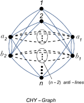
Figure 6: Graph representation for the CHY integrand, ${\bf I}^{\rm CHY}$, given in (13).

From the color code given in figure 4, we are considering all particles in figure 6 are massless, i.e. $k_{1}^{2}=\cdots=k_{n}^{2}=k_{a_{1}}^{2}=k_{a_{2}}^{2}=k_{b_{1}}^{2}=k_{b_{2}}^{2}=0$. So, we should use the original scattering equations formulated in Cachazo:2013hca ; Cachazo:2013iaa ; Cachazo:2013gna . These equations are given by the simple expressions

$$E_{A}=\sum_{B=1\atop B\neq A}^{n+4}\frac{k_{A}\cdot k_{B}}{\sigma_{AB}}=0,\qquad A=1,2,\ldots,n+4,$$ (14)

where we have identified

$$\{E_{n+1},E_{n+2},E_{n+3},E_{n+4}\} :=\{E_{a_{1}},E_{a_{2}},E_{b_{1}},E_{b_{2}}\},$$

$$\{\sigma_{n+1},\sigma_{n+2},\sigma_{n+3},\sigma_{n+4}\} :=\{\sigma_{a_{1}},\sigma_{a_{2}},\sigma_{b_{1}},\sigma_{b_{2}}\},$$ (15)

$$\{k_{n+1},k_{n+2},k_{n+3},k_{n+4}\} :=\{k_{a_{1}},k_{a_{2}},k_{b_{1}},k_{b_{2}}\},$$

and the momentum conservation constraint, $\sum_{A=1}^{n+4}k_{A}=\sum_{i=1}^{n}k_{i}+k_{a_{1}}+k_{a_{2}}+k_{b_{1}}+k_{b_{2}}=0$, is also satisfied.

Now, in order to obtain the $\Phi^{3}$ quadratic Feynman integrand at one-loop given in (10) from the original CHY approach, we propose the following formula

$$\mathfrak{I}^{\rm n-gon-CHY}_{\rm sym}:=\frac{1}{2^{n+1}}\int d\Omega\times(k_{a_{1}}+k_{b_{1}})^{2}\times\int d\mu\,\,\,\mathbf{I}^{\rm CHY},$$ (16)

where $\mathbf{I}^{\rm CHY}$ is the CHY integrand represented in figure 6 and given in (13), $d\mu$ is the original CHY tree-level meausre Cachazo:2013hca , namely

$$d\mu:= \frac{1}{{\rm Vol}\,\,({\rm PSL}(2,\mathbb{C}))}\times\prod_{A=1}^{n+4}\frac{d\sigma_{A}}{E_{A}}$$

$${}^{\underrightarrow{\,\quad{\rm fixing\,\,PSL}(2,\mathbb{C})\,\quad}}\,\,\,\frac{d\sigma_{a_{1}}}{E_{a_{1}}}\times\prod_{i=1}^{n}\frac{d\sigma_{i}}{E_{i}}\times(\sigma_{a_{2}b_{1}}\,\sigma_{b_{1}b_{2}}\,\sigma_{b_{2}a_{2}})^{2}$$ (17)

where, without loss of generality, we have fixed $\{\sigma_{a_{2}},\sigma_{b_{1}},\sigma_{b_{2}}\}$ and $\{E_{a_{2}},E_{b_{1}},E_{b_{2}}\}$, and $d\Omega$ is defined as

$$d\Omega: =d^{D}(k_{a_{1}}+k_{b_{1}})\,\delta^{(D)}(k_{a_{1}}+k_{b_{1}}-\ell)\,d^{D}k_{a_{2}}\,d^{D}k_{b_{2}}\,\delta^{(D)}(k_{a_{2}}+k_{a_{1}})\,\,\delta^{(D)}(k_{b_{2}}+k_{b_{1}}).$$ (18)

The Dirac delta functions, $\delta^{(D)}(k_{a_{2}}+k_{a_{1}})$ and $\delta^{(D)}(k_{b_{2}}+k_{b_{1}})$, are introduced to guarantee the forward limit, i.e. $k_{a_{2}}=-k_{a_{1}}$ and $k_{b_{2}}=-k_{b_{1}}$, and the last one, $\delta^{(D)}(k_{a_{1}}+k_{b_{1}}-\ell)$, is given to identify $k_{a_{1}}+k_{b_{1}}$ with the the loop momentum $\ell$, i.e the off-shell momentum $\ell$ is represented as a couple of massless particles.

Using the $\Lambda-$algorithm developed by the author in Gomez:2016bmv , we have verified, up to eight points, that in fact, the prescription proposed in (16) reproduces the quadratic Feynman integrand given in (10). So, we conjecture

$$\mathfrak{I}^{\rm n-gon-CHY}_{\rm sym} =\frac{1}{\ell^{2}\,(\ell+k_{1})^{2}(\ell+k_{1}+k_{2})^{2}\ldots(\ell-k_{n})^{2}}+{\rm Permutations\,\,}\{1,2,\ldots,n\}$$ (19)

$$=\frac{1}{\ell^{2}}\sum_{\alpha\in S_{n}}\frac{1}{(\ell+k_{\alpha_{1}})^{2}(\ell+k_{\alpha_{1}}+k_{\alpha_{2}})^{2}\ldots(\ell-k_{\alpha_{n}})^{2}}$$

$$={\cal I}^{\rm n-gon-FEY}_{\rm sym},$$

where $\alpha_{i}:=\alpha(i)$ and $S_{n}$ is the permutation group.

Remark.
Notice that we have been able to obtain the $\Phi^{3}$ quadratic Feynman integrand at one-loop from the CHY approach at tree-level and for massless particles. In addition, clearly the CHY-graphs in figures 6 can be obtained from the one given in figure 5, just by splitting the loop punctures in two on-shell particles. This is just a superficial fact, because the most interesting geometric consequences are going to be discussed in section 5.

General Diagram

Using the techniques presented by the author et al. in Cardona:2016wcr ; Gomez:2016cqb , the generalization for any $\Phi^{3}$ Feynman diagram is very simple. Schematically, the equivalence among any $\Phi^{3}$ Feynman diagram at one-loop and its corresponding CHY-graph is given in figure 7, where the symbol, $\mathsf{Sym}$, means symmetrization, namely a sum over all permutations of external legs.

    

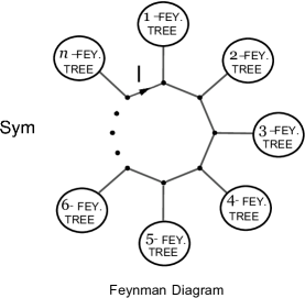
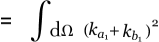
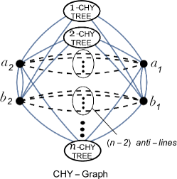
Figure 7: Schematic equivalence between the $\Phi^{3}$ general Feynman diagrams (symmetrized $n$-gon) and the CHY graphs.

As it was argued above, the equivalence in figure 7 is in fact an equality and the partial fraction identity is not necessary anymore. We will give a simple example in the next section.

4 Examples

In this section we consider three examples in order to check and illustrate the $\mathfrak{I}^{\rm n-gon-CHY}_{\rm sym}$ formula. We begin with the simplest one-loop case, the bubble. Latter, we will compute the triangle and finally an example of four-particle will be given, where we are going to use the generalization schematized in figure 7.

4.1 The Bubble

Let us consider the $\mathbf{I}^{\rm CHY}$ integrand given by expression

$$\mathbf{I}^{\rm CHY}=\frac{1}{(a_{1},b_{1},b_{2},a_{2})^{2}}\,\,(\omega^{a_{1}:a_{2}}_{1:2}\,\omega^{a_{1}:a_{2}}_{2:1})\times(\omega^{b_{1}:b_{2}}_{1:2}\,\omega^{b_{1}:b_{2}}_{2:1}).$$ (20)

Its CHY-graph is represented on the top in figure 8.

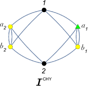
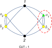
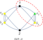
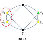
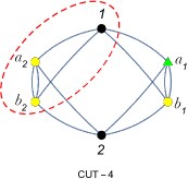
Figure 8: CHY-graph representation of ${\bf I}^{\rm CHY}$ written in (20). All possible non-zero cuts for ${\bf I}^{\rm CHY}$.

To perform the integral, $\int d\mu\,\mathbf{I}^{\rm CHY}$, we apply the $\Lambda-$algotihm developed in Gomez:2016bmv . So, the all possible non-zero cuts have been drawn on the second line in figure 8.

The computation of each cut is simple and the final answer for each one of them is

$$\mathbf{I}^{\rm CHY}_{\rm cut-1}= \frac{1}{k_{a_{1}b_{1}}}\left[\frac{1}{k_{1}\cdot(k_{a_{1}}+k_{b_{1}})}\times\frac{1}{k_{2}\cdot(k_{1}+k_{a_{1}}+k_{b_{1}})}+\frac{{\cal I}^{\rm 2-gon-CHY}_{\rm sym}(1,2|[a_{1},b_{1}],[a_{2},b_{2}])}{(k_{1}+k_{2})\cdot(k_{a_{1}}+k_{b_{1}})+k_{12}}\right],$$

$$\mathbf{I}^{\rm CHY}_{\rm cut-2}= \frac{1}{k_{1a_{1}b_{1}}}\times\frac{1}{k_{2}\cdot(k_{1}+k_{a_{1}}+k_{b_{1}})}\times\frac{1}{k_{1}\cdot(k_{2}+k_{a_{2}}+k_{b_{2}})},$$

$$\mathbf{I}^{\rm CHY}_{\rm cut-3}= \mathbf{I}^{\rm CHY}_{\rm cut-1}\Big{|}_{a_{1}\leftrightarrow a_{2}\atop b_{1}\leftrightarrow b_{2}},\qquad\mathbf{I}^{\rm CHY}_{\rm cut-4}=\mathbf{I}^{\rm CHY}_{\rm cut-2}\Big{|}_{a_{1}\leftrightarrow a_{2}\atop b_{1}\leftrightarrow b_{2}},$$

where ${\cal I}^{\rm 2-gon-CHY}_{\rm sym}(1,2|[a_{1},b_{1}],[a_{2},b_{2}])$ is the computation of the CHY-graph drawn in figure 9.

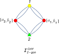
Figure 9: Graph representation for ${\cal I}^{\rm 2-gon-CHY}_{\rm sym}(1,2|[a_{1},b_{1}],[a_{2},b_{2}])$ (up to integration over the Moduli space, to wit $\int d\mu$).

Note that when $k_{a_{2}}+k_{b_{2}}=-(k_{a_{1}}+k_{b_{1}})$, namely on the support $\delta^{(D)}(k_{a_{2}}+k_{a_{1}})$ and $\delta^{(D)}(k_{b_{2}}+k_{b_{1}})$, the graph in figure 9 becomes one given in figure 5. However, on this support the denominator, $(k_{1}+k_{2})\cdot(k_{a_{1}}+k_{b_{1}})+k_{12}$, vanishes, i.e. there is a singularity. In fact, this is a spurious singularity, which can be removed using the momentum conservation condition, such as we are going to show. By summing, $\mathbf{I}^{\rm CHY}_{\rm cut-1}+\mathbf{I}^{\rm CHY}_{\rm cut-3}$, one obtains

$$\mathbf{I}^{\rm CHY}_{\rm cut-1}+\mathbf{I}^{\rm CHY}_{\rm cut-3}=$$ (21)

$$\frac{{\cal I}^{\rm 2-gon-CHY}_{\rm sym}(1,2|[a_{1},b_{1}],[a_{2},b_{2}])}{[(k_{1}+k_{2})\cdot(k_{a_{1}}+k_{b_{1}})+k_{12}]}\frac{2}{(k_{a_{1}}+k_{b_{1}})^{2}}+\frac{{\cal I}^{\rm 2-gon-CHY}_{\rm sym}(1,2|[a_{1},b_{1}],[a_{2},b_{2}])}{[(k_{1}+k_{2})\cdot(k_{a_{2}}+k_{b_{2}})+k_{12}]}\frac{2}{(k_{a_{2}}+k_{b_{2}})^{2}}+\cdots$$

where $``\cdots"$ means there are more terms. From the momentum conservation condition, $k_{1}+k_{2}+k_{a_{1}}+k_{b_{1}}+k_{a_{2}}+k_{b_{2}}=0$, it is easy to check

$$(k_{1}+k_{2})\cdot(k_{a_{1}}+k_{b_{1}})+k_{12}=-(k_{a_{1}}+k_{b_{1}}+k_{a_{2}}+k_{b_{2}})\cdot(k_{a_{1}}+k_{b_{1}})+\frac{1}{2}(k_{a_{1}}+k_{b_{1}}+k_{a_{2}}+k_{b_{2}})^{2}$$

$$=\frac{1}{2}\left[(k_{a_{2}}+k_{b_{2}})^{2}-(k_{a_{1}}+k_{b_{1}})^{2}\right]$$ (22)

and

$$(k_{1}+k_{2})\cdot(k_{a_{2}}+k_{b_{2}})+k_{12}=-(k_{a_{1}}+k_{b_{1}}+k_{a_{2}}+k_{b_{2}})\cdot(k_{a_{2}}+k_{b_{2}})+\frac{1}{2}(k_{a_{1}}+k_{b_{1}}+k_{a_{2}}+k_{b_{2}})^{2}$$

$$=-\frac{1}{2}\left[(k_{a_{2}}+k_{b_{2}})^{2}-(k_{a_{1}}+k_{b_{1}})^{2}\right].$$ (23)

Therefore, the sum in (21) becomes

$$\mathbf{I}^{\rm CHY}_{\rm cut-1}+\mathbf{I}^{\rm CHY}_{\rm cut-3} =\frac{2\,\,{\cal I}^{\rm 2-gon-CHY}_{\rm sym}(1,2|[a_{1},b_{1}],[a_{2},b_{2}])}{(k_{a_{2}}+k_{b_{2}})^{2}-(k_{a_{1}}+k_{b_{1}})^{2}}\left[\frac{2}{(k_{a_{1}}+k_{b_{1}})^{2}}-\frac{2}{(k_{a_{2}}+k_{b_{2}})^{2}}\right]+\cdots$$

$$=\frac{4\,\,{\cal I}^{\rm 2-gon-CHY}_{\rm sym}(1,2|[a_{1},b_{1}],[a_{2},b_{2}])}{(k_{a_{1}}+k_{b_{1}})^{2}\,\,(k_{a_{2}}+k_{b_{2}})^{2}}+\cdots$$ (24)

Clearly, the spurious pole on the support, $\delta^{(D)}(k_{a_{2}}+k_{a_{1}})\,\,\delta^{(D)}(k_{b_{2}}+k_{b_{1}})$, has been cleanly removed and we can now compute the integral $\int d\Omega$.

After removing the spurious pole and using the support, $\delta^{(D)}(k_{a_{2}}+k_{a_{1}})\,\,\delta^{(D)}(k_{b_{2}}+k_{b_{1}})$, it is straightforward to check

$$\mathbf{I}^{\rm CHY}_{\rm cut-1}+\mathbf{I}^{\rm CHY}_{\rm cut-2}+\mathbf{I}^{\rm CHY}_{\rm cut-3}+\mathbf{I}^{\rm CHY}_{\rm cut-4}=\frac{2}{k_{a_{1}b_{1}}k_{1a_{1}b_{1}}k_{2a_{1}b_{1}}}$$ (26)

$$=\frac{2^{4}}{(k_{a_{1}}+k_{b_{1}})^{2}(k_{1}+k_{a_{1}}+k_{b_{1}})^{2}(k_{2}+k_{a_{1}}+k_{b_{1}})^{2}}$$

$$=\frac{2^{3}}{(k_{a_{1}}+k_{b_{1}})^{2}}\left[\frac{1}{(k_{a_{1}}+k_{b_{1}})^{2}(k_{a_{1}}+k_{b_{1}}+k_{1})^{2}}+\frac{1}{(k_{a_{1}}+k_{b_{1}})^{2}(k_{a_{1}}+k_{b_{1}}+k_{2})^{2}}\right].$$

So, by computing the integral $\int d\Omega$, one obtains

$$\mathfrak{I}^{\rm 2-gon-CHY}_{\rm sym}= \int d\Omega\times\frac{(k_{a_{1}}+k_{b_{1}})^{2}}{2^{3}}\times\left(\mathbf{I}^{\rm CHY}_{\rm cut-1}+\mathbf{I}^{\rm CHY}_{\rm cut-2}+\mathbf{I}^{\rm CHY}_{\rm cut-3}+\mathbf{I}^{\rm CHY}_{\rm cut-4}\right)$$ (27)

$$= \frac{1}{\ell^{2}(\ell+k_{1})^{2}}+\frac{1}{\ell^{2}(\ell+k_{2})^{2}},$$

which is the Feynman integrand of the sum of diagrams given in figure 10, as it was expected.

Figure 10: Feynman diagram for the symmetrized Bubble .

4.2 The Triangle

As a second example we are going to consider the next case, the triangle.

Let $\mathbf{I}^{\rm CHY}$ be the CHY integrand represented by the graph in figure 11 and given by the analytic expression

$$\mathbf{I}^{\rm CHY}=\frac{1}{(a_{1},b_{1},b_{2},a_{2})^{2}}\,\,(\omega^{a_{1}:a_{2}}_{1:2}\,\omega^{a_{1}:a_{2}}_{2:3}\,\omega^{a_{1}:a_{2}}_{3:1})\times(\omega^{b_{1}:b_{2}}_{1:3}\,\omega^{b_{1}:b_{2}}_{3:2}\,\omega^{b_{1}:b_{2}}_{2:1}).$$ (28)

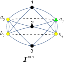
Figure 11: CHY-graph of the ${\bf I}^{\rm CHY}$ integrand given in (28).

In order to compute $\int d\mu\,\,\mathbf{I}^{\rm CHY}$, we use the $\Lambda-$algorithm. So, in figure 12 we have drawn the all possible non-zero cuts.

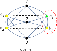
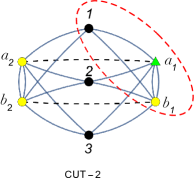
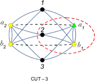
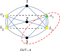
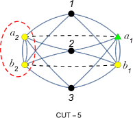
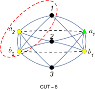
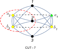
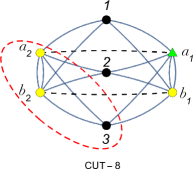
Figure 12: All possible non-zero cuts.

The computations are not hard and the final answer for each cut is

$$\mathbf{I}^{\rm CHY}_{\rm cut-1}=\frac{1}{k_{a_{1}b_{1}}}\left\{\frac{1}{k_{1}\cdot(k_{a_{1}}+k_{b_{1}})}\left[\frac{1}{k_{2}\cdot(k_{1}+k_{a_{1}}+k_{b_{1}})}\times\frac{1}{k_{3}\cdot(k_{1}+k_{2}+k_{a_{1}}+k_{b_{1}})}\right.\right.$$

$$\left.+\frac{B(\{3\},\{2\},\{1,a_{1},b_{1}\},\{a_{2},b_{2}\})}{(k_{2}+k_{3})(k_{1}+k_{a_{1}}+k_{b_{1}})+k_{23}}\right]+\frac{1}{(k_{1}+k_{2})\cdot(k_{a_{1}}+k_{b_{1}})+k_{12}}\times\frac{B(\{2\},\{1\},\{a_{1},b_{1}\},\{3,a_{2},b_{2}\})}{k_{3}\cdot(k_{1}+k_{2}+k_{a_{1}}+k_{b_{1}})}$$

$$+\frac{1}{(k_{1}+k_{3})\cdot(k_{a_{1}}+k_{b_{1}})+k_{13}}\times\frac{B(\{3\},\{1\},\{a_{1},b_{1}\},\{2,a_{2},b_{2}\})}{k_{2}\cdot(k_{1}+k_{3}+k_{a_{1}}+k_{b_{1}})}\left.+\frac{{\cal I}^{\rm 3-gon-CHY}_{\rm sym}(1,2,3|[a_{1},b_{1}],[a_{2},b_{2}])}{(k_{1}+k_{2}+k_{3})\cdot(k_{a_{1}}+k_{b_{1}})+k_{123}}\right\},$$

$$\mathbf{I}^{\rm CHY}_{\rm cut-2}=\frac{1}{k_{1a_{1}b_{1}}}\left\{\frac{1}{k_{1}\cdot(k_{2}+k_{3}+k_{a_{2}}+k_{b_{2}})}\times\left[\frac{1}{k_{2}\cdot(k_{1}+k_{a_{1}}+k_{b_{1}})}\times\frac{1}{k_{3}\cdot(k_{1}+k_{2}+k_{a_{1}}+k_{b_{1}})}\right.\right.$$

$$\left.\left.+\frac{B(\{3\},\{2\},\{1,a_{1},b_{1}\},\{a_{2},b_{2}\})}{(k_{2}+k_{3})\cdot(k_{1}+k_{a_{1}}+k_{b_{1}})+k_{23}}\right]\right\},$$

$$\mathbf{I}^{\rm CHY}_{\rm cut-3}=\mathbf{I}^{\rm CHY}_{\rm cut-2}\Big{|}_{k_{1}\leftrightarrow k_{2}},\qquad\mathbf{I}^{\rm CHY}_{\rm cut-4}=\mathbf{I}^{\rm CHY}_{\rm cut-2}\Big{|}_{k_{1}\leftrightarrow k_{3}},\qquad\mathbf{I}^{\rm CHY}_{\rm cut-5}=\mathbf{I}^{\rm CHY}_{\rm cut-1}\Big{|}_{a_{1}\leftrightarrow a_{2}\atop b_{1}\leftrightarrow b_{2}},$$

$$\mathbf{I}^{\rm CHY}_{\rm cut-6}=\mathbf{I}^{\rm CHY}_{\rm cut-2}\Big{|}_{a_{1}\leftrightarrow a_{2}\atop b_{1}\leftrightarrow b_{2}},\qquad\mathbf{I}^{\rm CHY}_{\rm cut-7}=\mathbf{I}^{\rm CHY}_{\rm cut-3}\Big{|}_{a_{1}\leftrightarrow a_{2}\atop b_{1}\leftrightarrow b_{2}},\qquad\mathbf{I}^{\rm CHY}_{\rm cut-8}=\mathbf{I}^{\rm CHY}_{\rm cut-4}\Big{|}_{a_{1}\leftrightarrow a_{2}\atop b_{1}\leftrightarrow b_{2}},$$

where ${\cal I}^{\rm 3-gon-CHY}_{\rm sym}(1,2,3|[a_{1},b_{1}],[a_{2},b_{2}])$ is the computation of the CHY-graph given in figure 13.

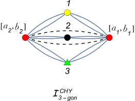
Figure 13: CHY-graph representation for ${\cal I}^{\rm 3-gon-CHY}_{\rm sym}(1,2,3|[a_{1},b_{1}],[a_{2},b_{2}])$, up to integral over the Moduli space, i.e. $\int d\mu$.

Clearly, such as it happened in the previous example, there is a spurious pole when the support, $\delta^{(D)}(k_{a_{2}}+k_{a_{1}})\,\,\delta^{(D)}(k_{b_{2}}+k_{b_{1}})$, is considered, i.e. the cuts $\mathbf{I}^{\rm CHY}_{\rm cut-1}$ and $\mathbf{I}^{\rm CHY}_{\rm cut-5}$ become infinite when $k_{a_{2}}=-k_{a_{1}}$ and $k_{b_{2}}=-k_{b_{1}}$. In order to remove it, we apply the same trick as in section 4.1. So, by considering the sum, $\mathbf{I}^{\rm CHY}_{\rm cut-1}+\mathbf{I}^{\rm CHY}_{\rm cut-5}$, and using the momentum conservation condition, such as in (4.1) and (4.1), it is straightforward to check

$$\mathbf{I}^{\rm CHY}_{\rm cut-1}+\mathbf{I}^{\rm CHY}_{\rm cut-5}=\frac{4\,\,{\cal I}^{\rm 3-gon-CHY}_{\rm sym}(1,2,3|[a_{1},b_{1}],[a_{2},b_{2}])}{(k_{a_{1}}+k_{b_{1}})^{2}\,\,(k_{a_{2}}+k_{b_{2}})^{2}}+\ldots,$$

and therefore the spurious singularity on $\delta^{(D)}(k_{a_{2}}+k_{a_{1}})\,\,\delta^{(D)}(k_{b_{2}}+k_{b_{1}})$ is removed.

Finally, after removing the spurious pole and on the support, $\delta^{(D)}(k_{a_{2}}+k_{a_{1}})\,\,\delta^{(D)}(k_{b_{2}}+k_{b_{1}})$, one can verify

$$\sum_{i=1}^{8}{\bf I}^{\rm CHY}_{{\rm cut-}i} =\frac{2^{4}}{s_{a_{1}b_{1}}}\left[\frac{1}{s_{a_{1}b_{1}}\,(k_{a_{1}}+k_{b_{1}}+k_{1})^{2}\,(k_{a_{1}}+k_{b_{1}}+k_{1}+k_{2})^{2}}+{\rm Permutations}\,\,\{1,2,3\}\right]$$

$$=\frac{2^{4}}{s_{a_{1}b_{1}}}\sum_{\alpha\in S_{3}}\frac{1}{s_{a_{1}b_{1}}\,(k_{a_{1}}+k_{b_{1}}+k_{\alpha_{1}})^{2}\,(k_{a_{1}}+k_{b_{1}}+k_{\alpha_{1}}+k_{\alpha_{2}})^{2}}.$$ (29)

Therefore, by integrating $\int\,d\Omega$, it is simple to see

$$\mathfrak{I}^{\rm 3-gon-CHY}_{\rm sym} =\int d\Omega\times\frac{(k_{a_{1}}+k_{b_{1}})^{2}}{2^{4}}\times\left(\sum_{i=1}^{8}{\bf I}^{\rm CHY}_{{\rm cut-}i}\right)$$

$$=\frac{1}{\ell^{2}(\ell+k_{1})^{2}\,(\ell+k_{1}+k_{2})^{2}}+{\rm Permutations\,\{1,2,3\}}$$

$$=\sum_{\alpha\in S_{3}}\frac{1}{\ell^{2}\,(\ell+k_{\alpha_{1}})^{2}\,(\ell+k_{\alpha_{1}}+k_{\alpha_{2}})^{2}},$$ (30)

which is the Feynman integrand of the six diagrams given in figure 14, as it was expected.

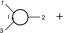
Figure 14: Feynman diagram for the symmetrized Triangle.

4.3 Four-particle

In this section we look upon a more complicated example, a four-particle computation. In order to present an example with the same structure as in figure 7, we consider a triangle with four-particle.

Let ${\bf I}^{\rm CHY}$ be the CHY integrand given by

$$\mathbf{I}^{\rm CHY}=\frac{1}{(a_{1},b_{1},b_{2},a_{2})^{2}}\,\,(\omega^{a_{1}:a_{2}}_{1:2}\,\frac{1}{\sigma_{23}}\,\omega^{a_{1}:a_{2}}_{3:4}\,\omega^{a_{1}:a_{2}}_{4:1})\times(\omega^{b_{1}:b_{2}}_{1:4}\,\omega^{b_{1}:b_{2}}_{4:3}\,\frac{1}{\sigma_{32}}\,\omega^{b_{1}:b_{2}}_{2:1}),$$ (31)

and in figure 15 we have represented its CHY-graph.

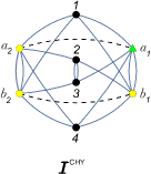
Figure 15: CHY-graph of the integrand in (31)

The computation of the integral, $\int d\mu\,{\bf I}^{\rm CHY}$, is performed by applying the $\Lambda-$algorithm. Following this algorithm, we draw the all possible non-zero cuts in figure 16.

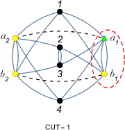
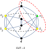
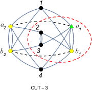
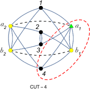
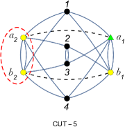
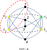
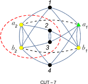
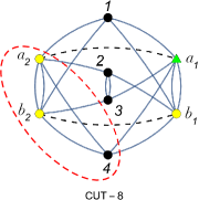
Figure 16: All possible non-zero cuts.

The answer of each cut is obtained after a long but not hard computation and the final results are given by the expressions

$$\mathbf{I}^{\rm CHY}_{\rm cut-1}= \frac{1}{k_{23}\,\,k_{a_{1}b_{1}}}\left\{\frac{1}{k_{1}\cdot(k_{a_{1}}+k_{b_{1}})}\left[\frac{1}{(k_{2}+k_{3})\cdot(k_{1}+k_{a_{1}}+k_{b_{1}})+k_{23}}\times\frac{1}{k_{4}\cdot(k_{1}+k_{2}+k_{3}+k_{a_{1}}+k_{b_{1}})}\right.\right.$$

$$\left.+\frac{B(\{4\},\{2,3\},\{1,a_{1},b_{1}\},\{a_{2},b_{2}\})}{(k_{2}+k_{3}+k_{4})(k_{1}+k_{a_{1}}+k_{b_{1}})+k_{234}}\right]$$

$$+\frac{1}{(k_{1}+k_{2}+k_{3})\cdot(k_{a_{1}}+k_{b_{1}})+k_{123}}\times\frac{B(\{2,3\},\{1\},\{a_{1},b_{1}\},\{4,a_{2},b_{2}\})}{k_{4}\cdot(k_{1}+k_{2}+k_{3}+k_{a_{1}}+k_{b_{1}})}$$

$$+\frac{1}{(k_{1}+k_{4})\cdot(k_{a_{1}}+k_{b_{1}})+k_{14}}\times\frac{B(\{4\},\{1\},\{a_{1},b_{1}\},\{2,3,a_{2},b_{2}\})}{(k_{2}+k_{3})\cdot(k_{1}+k_{4}+k_{a_{1}}+k_{b_{1}})+k_{23}}$$

$$\left.+\frac{k_{23}\,\,{\cal I}^{\rm CHY}_{\rm 4-Triangle}(1|2,3|4|[a_{1},b_{1}],[a_{2},b_{2}])}{(k_{1}+k_{2}+k_{3}+k_{4})\cdot(k_{a_{1}}+k_{b_{1}})+k_{1234}}\right\},$$

$$\mathbf{I}^{\rm CHY}_{\rm cut-2}= \frac{1}{k_{23}\,k_{1a_{1}b_{1}}}\times\frac{1}{k_{1}\cdot(k_{2}+k_{3}+k_{4}+k_{a_{2}}+k_{b_{2}})}\times$$

$$\left[\frac{1}{(k_{2}+k_{3})\cdot(k_{1}+k_{a_{1}}+k_{b_{1}})+k_{23}}\times\frac{1}{k_{4}\cdot(k_{1}+k_{2}+k_{3}+k_{a_{1}}+k_{b_{1}})}\right.$$

$$\left.+\frac{B(\{4\},\{2,3\},\{1,a_{1},b_{1}\},\{a_{2},b_{2}\})}{(k_{2}+k_{3}+k_{4})\cdot(k_{1}+k_{a_{1}}+k_{b_{1}})+k_{234}}\right],$$

$$\mathbf{I}^{\rm CHY}_{\rm cut-3}= \frac{1}{k_{23}\,k_{23a_{1}b_{1}}}\times\frac{1}{(k_{2}+k_{3})\cdot(k_{1}+k_{4}+k_{a_{2}}+k_{b_{2}})+k_{23}}\times$$

$$\left[\frac{1}{k_{1}\cdot(k_{2}+k_{3}+k_{a_{1}}+k_{b_{1}})}\times\frac{1}{k_{4}\cdot(k_{1}+k_{2}+k_{3}+k_{a_{1}}+k_{b_{1}})}\right.$$

$$\left.+\frac{B(\{4\},\{1\},\{2,3,a_{1},b_{1}\},\{a_{2},b_{2}\})}{(k_{1}+k_{4})\cdot(k_{2}+k_{3}+k_{a_{1}}+k_{b_{1}})+k_{14}}\right],$$

$$\mathbf{I}^{\rm CHY}_{\rm cut-4}=\mathbf{I}^{\rm CHY}_{\rm cut-2}\Big{|}_{k_{1}\leftrightarrow k_{4}},\qquad\mathbf{I}^{\rm CHY}_{\rm cut-5}=\mathbf{I}^{\rm CHY}_{\rm cut-1}\Big{|}_{a_{1}\leftrightarrow b_{2}\atop b_{1}\leftrightarrow a_{2}},\qquad\mathbf{I}^{\rm CHY}_{\rm cut-6}=\mathbf{I}^{\rm CHY}_{\rm cut-2}\Big{|}_{a_{1}\leftrightarrow b_{2}\atop b_{1}\leftrightarrow a_{2}}$$

$$\mathbf{I}^{\rm CHY}_{\rm cut-7}=\mathbf{I}^{\rm CHY}_{\rm cut-3}\Big{|}_{a_{1}\leftrightarrow b_{2}\atop b_{1}\leftrightarrow a_{2}},\qquad\mathbf{I}^{\rm CHY}_{\rm cut-8}=\mathbf{I}^{\rm CHY}_{\rm cut-4}\Big{|}_{a_{1}\leftrightarrow b_{2}\atop b_{1}\leftrightarrow a_{2}},$$

where ${\cal I}^{\rm CHY}_{\rm 4-Triangle}(1|2,3|4|[a_{1},b_{1}],[a_{2},b_{2}])$ is the computation of the CHY graph in figure 17.

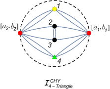
Figure 17: CHY-graph for ${\cal I}^{\rm CHY}_{\rm 4-Triangle}(1|2,3|4|[a_{1},b_{1}],[a_{2},b_{2}])$, up to integral over the Moduli space, i.e. $\int d\mu$.

As it happened in the above examples, the cuts, $\mathbf{I}^{\rm CHY}_{\rm cut-1}$ and $\mathbf{I}^{\rm CHY}_{\rm cut-5}$, have spurious pole on $\delta^{(D)}(k_{a_{2}}+k_{a_{1}})\,\,\delta^{(D)}(k_{b_{2}}+k_{b_{1}})$. In order to remove it, we consider the sum, $\mathbf{I}^{\rm CHY}_{\rm cut-1}+\mathbf{I}^{\rm CHY}_{\rm cut-5}$. Using the momentum conservation condition, such as in (4.1) and (4.1), it is straightforward to see

$$\mathbf{I}^{\rm CHY}_{\rm cut-1}+\mathbf{I}^{\rm CHY}_{\rm cut-5}=\frac{4\,\,{\cal I}^{\rm CHY}_{\rm 4-Triangle}(1|2,3|4|[a_{1},b_{1}],[a_{2},b_{2}])}{(k_{a_{1}}+k_{b_{1}})^{2}\,\,(k_{a_{2}}+k_{b_{2}})^{2}}+\ldots,$$

and therefore the spurious pole on the support $\delta^{(D)}(k_{a_{2}}+k_{a_{1}})\,\,\delta^{(D)}(k_{b_{2}}+k_{b_{1}})$ is eliminated.

Unlike the bubble and triangle examples, the term ${\cal I}^{\rm CHY}_{\rm 4-Triangle}(1|2,3|4|[a_{1},b_{1}],[a_{2},b_{2}])$ does not vanish when $k_{a_{2}}=-k_{a_{1}}$ and $k_{b_{2}}=-k_{b_{1}}$, and its result is given by

$${\cal I}^{\rm CHY}_{\rm 4-Triangle}(1|2,3|4|[a_{1},b_{1}],[a_{2},b_{2}])=\frac{1}{k_{23}}\times$$

$$\left\{\frac{B(\{2,3\},\{4\},\{1,a_{1},b_{1}\},\{a_{2},b_{2}\})}{(k_{2}+k_{3}+k_{4})\cdot(k_{a_{2}}+k_{b_{2}})+k_{234}}+\frac{B(\{2,3\},\{4\},\{1,a_{2},b_{2}\},\{a_{1},b_{1}\})}{(k_{2}+k_{3}+k_{4})\cdot(k_{a_{1}}+k_{b_{1}})+k_{234}}\right.$$

$$\left.+\frac{B(\{2,3\},\{1\},\{4,a_{1},b_{1}\},\{a_{2},b_{2}\})}{k_{4}\cdot(k_{a_{1}}+k_{b_{1}})}+\frac{B(\{2,3\},\{1\},\{4,a_{2},b_{2}\},\{a_{1},b_{1}\})}{k_{4}\cdot(k_{a_{2}}+k_{b_{2}})}\right\}.$$

Finally, after removing the spurious pole and on the support, $\delta^{(D)}(k_{a_{2}}+k_{a_{1}})\,\,\delta^{(D)}(k_{b_{2}}+k_{b_{1}})$, one can show

$$\sum_{i=1}^{8}{\bf I}^{\rm CHY}_{{\rm cut-}i} =\frac{2^{5}}{s_{a_{1}b_{1}}}\times\frac{1}{s_{23}\,s_{a_{1}b_{1}}\,(k_{a_{1}}+k_{b_{1}}+k_{1})^{2}\,(k_{a_{1}}+k_{b_{1}}+k_{1}+k_{\{2,3\}})^{2}}+{\rm Permutations}\{1,\{2,3\},4\}$$

$$=\frac{2^{5}}{s_{a_{1}b_{1}}}\times\sum_{p\in P_{3}}\frac{1}{(k_{2}+k_{3})^{2}\,(k_{a_{1}}+k_{b_{1}})^{2}\,(k_{a_{1}}+k_{b_{1}}+k_{p_{1}})^{2}\,(k_{a_{1}}+k_{b_{1}}+k_{p_{1}}+k_{p_{2}})^{2}}$$

where $P_{3}$ is defined as

$$P_{3}:={\rm permutations}\,\{\beta_{1},\beta_{2},\beta_{3}\},\qquad{\rm with}~{}~{}\beta_{1}:=1\,,\beta_{2}:=\{2,3\}\,,\beta_{3}:=4,$$ (32)

for example, $k_{\beta_{2}}=k_{\{2,3\}}=k_{2}+k_{3}$.

Therefore, by integrating $\int\,d\Omega$ one obtains

$$\mathfrak{I}^{\rm 3-gon-CHY}_{\rm sym} =\int d\Omega\times\frac{(k_{a_{1}}+k_{b_{1}})^{2}}{2^{5}}\times\left(\sum_{i=1}^{8}{\bf I}^{\rm CHY}_{{\rm cut-}i}\right)$$

$$=\frac{1}{s_{23}\,\ell^{2}\,(\ell+k_{1})^{2}\,(\ell+k_{1}+k_{\{2,3\}})^{2}}+{\rm Permutations\,\{1,\{2,3\},4\}}$$

$$=\frac{1}{s_{23}}\sum_{p\in P_{3}}\frac{1}{\ell^{2}\,(\ell+k_{p_{1}})^{2}\,(\ell+k_{p_{1}}+k_{p_{2}})^{2}},$$ (33)

which is the Feynman integrand of the sum of diagrams given in figure 18, as it was expected.

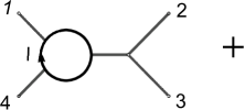
Figure 18: Symmetrized Feynman diagram of the Triangle with four particles.

5 Discussions

In this paper we have presented a new proposal in order to obtain the quadratic Feynman integrand at one-loop from the CHY approach. We have focused our research just to $\Phi^{3}$ theory, which is the simplest case, nevertheless, we have already obtained some progress by extending our ideas to other theories wp .

Note that our proposal is totally different to ones knew so far Geyer:2015bja ; Geyer:2015jch ; Adamo:2013tsa ; Baadsgaard:2015hia ; He:2015yua ; Cachazo:2015aol ; Chen:2016fgi ; Chen:2017edo ; Cardona:2016bpi ; Cardona:2016wcr . Basically, in all of these papers, the CHY approach of $n-$particles at one-loop is given by a contour integral over the moduli space of $(n+2)-$punctured spheres with two off-shell particles in the forward limit (the internal loop momentum), and the final answer is obtained in the ${\cal Q}-$cut language Baadsgaard:2015twa , such as in section 2. In contrast, our formula is given by an integral over the moduli space of $(n+4)-$punctured spheres and the all particles are massless (section 3). This is the first proposal where the CHY approach is able to obtained cleanly a quadratic Feynman integrand at loop-level, i.e. without to use the partial fraction identity nor shifting the internal loop momentum.

Schematically, one can say that our proposal is based on the idea that each internal loop puncture is interpreted as a couple of massless particles. This is the reason why a CHY-graph at one-loop, such as one drew in figure 5, always appears in the computation, which is multiplied by a spurious pole that becomes singular on the support, $\delta^{(D)}(k_{a_{2}}+k_{a_{1}})\,\delta^{(D)}(k_{b_{2}}+k_{b_{1}})$, such as it was shown in the examples in section 4. However, our really motivation comes from the CHY prescription at two-loop developed by the author et al in Gomez:2016cqb .

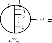
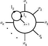
Figure 19: $\Phi^{3}$ Feynman diagram at two-loop.

To understand the idea, let us consider the $\Phi^{3}$ Feynman diagram at two-loop given in figure 19, which has as integrand

$${\cal I}_{\rm 2-loop}^{\rm FEY}=\frac{1}{\ell_{1}^{2}\,\ell_{2}^{2}\,(\ell_{1}-k_{n+1})^{2}}\sum_{\alpha\in S_{n}}\frac{1}{(\ell_{1}+\ell_{2})^{2}\,(\ell_{1}+\ell_{2}+k_{\alpha_{1}})^{2}\,\cdots(\ell_{1}+\ell_{2}+k_{\alpha_{1}}+\cdot+k_{\alpha_{n}})^{2}}.$$

Following the rules and building blocks given by the author et al in Gomez:2016cqb , the corresponding CHY-integral that reproduces the ${\cal I}_{\rm 2-loop}^{\rm FEY}$ integrand, after partial fraction identity and shifting the loop momentum, is given by the expression

$${\cal I}_{\rm 2-Loop}^{\rm CHY} =\frac{1}{\ell_{1}^{2}\,\ell_{2}^{2}}\int\,d\mu^{\rm 2-Loop}\,{\bf I}^{\rm CHY}_{\rm 2-Loop},$$ (34)

$${\bf I}_{\rm 2-Loop}^{\rm CHY} =\frac{1}{(\ell_{1}^{+},\ell_{2}^{+},\ell_{2}^{-},\ell_{2}^{-})^{2}}\,\,\left(\omega_{1:2}^{\ell_{1}^{+}:\ell_{1}^{-}}\cdots\omega_{n-1:n}^{\ell_{1}^{+}:\ell_{1}^{-}}\,\omega_{n:1}^{\ell_{1}^{+}:\ell_{1}^{-}}\right)\times\left(\omega_{1:n}^{\ell_{2}^{+}:\ell_{2}^{-}}\,\omega_{n:n-1}^{\ell_{2}^{+}:\ell_{2}^{-}}\cdots\omega_{2:1}^{\ell_{2}^{+}:\ell_{2}^{-}}\right)$$

$$\qquad\qquad\qquad\quad\quad\times\omega_{n+1:n+1}^{\ell_{1}^{+}:\ell_{1}^{-}}\left(\omega_{n+1:n+1}^{\ell_{1}^{+}:\ell_{1}^{-}}-\omega_{n+1:n+1}^{\ell_{2}^{+}:\ell_{2}^{-}}\right),$$

where the measure $d\mu^{\rm 2-loop}$ is defined in Geyer:2016wjx ; Gomez:2016cqb and the ${\bf I}_{\rm 2-Loop}^{\rm CHY}$ integrand is represented graphically in figure 20.

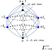
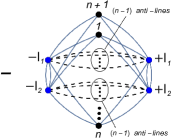
Figure 20: CHY-graph representation for the ${\bf I}^{\rm CHY}_{\rm 2-Loop}$ integrand in (34).

In Gomez:2016cqb , it was argued that after carrying out the (34) integral, then ${\cal I}_{\rm 2-Loop}^{\rm CHY}$ becomes

$${\cal I}_{\rm 2-Loop}^{\rm CHY} =\frac{2^{n}}{\ell_{1}^{2}\,\ell_{2}^{2}\,(-\ell_{1}\cdot k_{n+1})}\sum_{\alpha\in S_{n}}\frac{1}{(\ell_{1}+\ell_{2})^{2}\,(\ell_{1}+\ell_{2}+k_{\alpha_{1}})^{2}\,\cdots(\ell_{1}+\ell_{2}+k_{\alpha_{1}}+\cdots+k_{\alpha_{n}})^{2}}$$

$$\quad+\frac{2^{n}}{\ell_{1}^{2}\,\ell_{2}^{2}\,(\ell_{1}\cdot k_{n+1})}\sum_{\alpha\in S_{n}}\frac{1}{(\ell_{1}+\ell_{2})^{2}\,(\ell_{1}+\ell_{2}-k_{\alpha_{1}})^{2}\,\cdots(\ell_{1}+\ell_{2}-k_{\alpha_{1}}-\cdots-k_{\alpha_{n}})^{2}}.$$

It is straightforward to check that using the partial fraction identity over the factor, $\frac{1}{\ell_{1}^{2}(\ell_{1}-k_{n+1})^{2}}$, in ${\cal I}_{\rm 2-Loop}^{\rm FEY}$ and by shifting the $\ell_{1}^{\mu}$ loop momentum, one obtains ${\cal I}_{\rm 2-Loop}^{\rm CHY}$.

Note that the CHY-integral in (34) is able to produce some quadratic Feynman propagators, to be more precise, the propagators that are on the middle line in the Feynman diagram drawn in figure 20. So, in order to obtain just quadratic Feynman propagators, one can naively think in the CHY-graph given in figure 21.

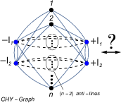
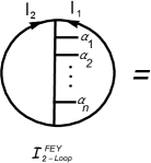
Figure 21: CHY-graph that naively would be able to produce just quadratic Feynman propagators.

Nevertheless, an equivalence among the CHY-graph (left side) and the Feynman diagram (right side) in figure 21 is not established, because the CHY-graph is singular. From the $\Lambda-$algorithm point of view this means there are divergent cuts, for example the one given in figure 22. This singular cut is obtained by cutting $(\ell_{1}^{+},\ell_{2}^{+})$ and latter $(\ell_{1}^{-},\ell_{2}^{-})$, which generates a CHY-graph at one-loop as in figure 5, times the infinite propagator, $\frac{1}{(\ell_{1}+\ell_{2})\cdot(k_{1}+\ldots+k_{n})+k_{1\cdots n}}$.

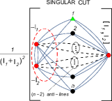
Figure 22: Singular cut (Tacnode singularity).

Notice that each CHY-graph in figure 20 generates also these kind of singular cuts, but they are canceled out by the linear combination between the graphs, which does not happen with the one in figure 21.
The geometrical meaning of this singularity can be studied from a hyper-elliptic curve of genus two. Let us consider the complex curve

$$y^{2}=z(z-1)(z-\lambda_{1})(z-\lambda_{2})(z-\lambda_{3}),$$ (35)

where $(\lambda_{1},\lambda_{2},\lambda_{3})$ parameterizes the Moduli space (${\cal M}_{2}$) of this curve. If $\lambda_{1}=0$ and $\lambda_{2}=1$ then the curve is degenerated to a sphere with four punctures and the parameter, $\lambda_{3}$, can be used to perform the $\Lambda-$algorithm. This singularity is known as node singularity, which is equivalent to pinching two $A-$cycles, and it gives arisen to CHY-graphs as ones drawn in figure 20 and 21. Other type of singularity is, for example, when $\lambda_{1}=\lambda_{2}=\lambda_{3}=0$, which is known as tacnode singularity. These singularities generate CHY-graphs as one given in figure 22, which has a propagator trivially infinite by momentum conservation, for instance $\frac{1}{(\ell_{1}+\ell_{2})\cdot(k_{1}+\ldots+k_{n})+k_{1\cdots n}}$. So, to cancel out the tacnode singularities we consider a linear combination of graphs, as in figure 20 Gomez:2016cqb . But, clearly the CHY-graph in figure 21 is not able to do that. Finally, the other types of singularities do not appear in the computation, so we do not consider them here.

Our proposal is supported and motivated on the above ideas at two-loop Gomez:2016cqb . Since we just wish obtained quadratic Feynman propagators, then it is natural to think over the CHY-graph in figure 21, again. But, so as to avoid the tacnode singularities, we consider all particles are differents, namely their momenta are generic. Naively, one could try to apply this trick on the graph in figure 21, and then making the forward limit, however, it could break the ${\rm PSL}(2,\mathbb{C})$ invariance of the scattering equations at two-loop. In order to solve this drawback we regard the all particles are massless and therefore the scattering equations are the original ones given in Cachazo:2013hca ; Cachazo:2013iaa ; Cachazo:2013gna . Now, to obtain a loop we should come back to try a forward limit, but, it generates a propagator trivially infinite multiplied by the tacnode singularity contribution, as it was seen previously. As we have shown in section 4, this infinite propagator is in fact a fake infinity, which can be removed using the momentum conservation condition before making the forward limit. Therefore, we now are able to perform, transparently, the forward limit and, unlike with the two-loop case, the tacnode singularity is going to contribute to the computation. Finally, in order to obtain an internal loop we need an off-shell momentum. So, since the on-shell momenta related with the punctures generated by the node singularities, in figure 23 they are $(a_{1},b_{1})$ and $(a_{2},b_{2})$, are always together as a couple, then we may identify this couple with an off-shell loop momentum, i.e. we are going to obtain an amplitude at one-loop.

 

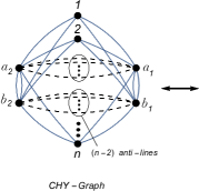
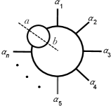
Figure 23: Feynman diagram meaning for the new CHY proposal .

In conclusion, we have developed a technique to obtain quadratic Feynman propagators at one-loop from a Riemann surfaces of genus two by performing an unitary cut, such as it is shown in figure 23, where $d\Omega$ is the meausre defined in (18). Therefore, if we wish to obtain the exact quadratic Feynman integrand at two-loop given in (5), we should perform an unitary cut on a Riemann surface of genus four, as we schematized in figure 24. Roughly speaking, this means that each off-shell puncture in figure 20 should be splitting in two massless punctures wp .

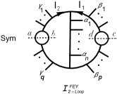
Figure 24: Representation of the process to obtain quadratic Feynman propagators at two-loop. ${\rm Sym}$ means sum over all permutations for each set of external legs.

On the other hand, since the most of relationship among scattering amplitudes have been deeply studied at tree-level, such as the Bern-Carrasco-Johansson (BCJ) relations, the Kawai–Lewellen–Tye (KLT) kernel, monodromy relations or the soft limit behavior Bern:2008qj ; Kawai:1985xq ; He:2016mzd ; Tourkine:2016bak ; Bjerrum-Bohr:2016axv ; Bjerrum-Bohr:2016juj ; Huang:2017ydz ; Teng:2017tbo ; He:2016vfi ; Schwab:2014xua ; Cachazo:2015ksa ; Kalousios:2014uva ; Afkhami-Jeddi:2014fia ; Cachazo:2016njl ; Stieberger:2016lng ; Hohenegger:2017kqy , then following the ideas presented in this paper, where we have developed a technique to write scattering amplitudes of $n-$particles at one-loop as amplitudes of $(n+4)-$particles at tree-level, we are confident that it is possible to apply the whole knowledge obtained at tree-level to find new relationships at loop-level.

- (1) E. Witten, Perturbative gauge theory as a string theory in twistor space, Commun. Math. Phys. 252 (2004) 189–258, [hep-th/0312171].
- (2) F. Cachazo, S. He and E. Y. Yuan, Scattering equations and Kawai-Lewellen-Tye orthogonality, Phys.Rev. D90 (2014) 065001, [1306.6575].
- (3) F. Cachazo, S. He and E. Y. Yuan, Scattering of Massless Particles in Arbitrary Dimensions, Phys.Rev.Lett. 113 (2014) 171601, [1307.2199].
- (4) F. Cachazo, S. He and E. Y. Yuan, Scattering in Three Dimensions from Rational Maps, JHEP 10 (2013) 141, [1306.2962].
- (5) F. Cachazo, S. He and E. Y. Yuan, Scattering of Massless Particles: Scalars, Gluons and Gravitons, JHEP 1407 (2014) 033, [1309.0885].
- (6) F. Cachazo, S. He and E. Y. Yuan, Scattering Equations and Matrices: From Einstein To Yang-Mills, DBI and NLSM, 1412.3479.
- (7) F. Cachazo, S. He and E. Y. Yuan, Einstein-Yang-Mills Scattering Amplitudes From Scattering Equations, JHEP 1501 (2015) 121, [1409.8256].
- (8) F. Cachazo, P. Cha and S. Mizera, Extensions of Theories from Soft Limits, JHEP 06 (2016) 170, [1604.03893].
- (9) R. Roiban, M. Spradlin and A. Volovich, On the tree level S matrix of Yang-Mills theory, Phys. Rev. D70 (2004) 026009, [hep-th/0403190].
- (10) F. Cachazo and Y. Geyer, A ‘Twistor String’ Inspired Formula For Tree-Level Scattering Amplitudes in N=8 SUGRA, 1206.6511.
- (11) F. Cachazo and D. Skinner, Gravity from Rational Curves in Twistor Space, Phys. Rev. Lett. 110 (2013) 161301, [1207.0741].
- (12) H. Kawai, D. C. Lewellen and S. H. H. Tye, A Relation Between Tree Amplitudes of Closed and Open Strings, Nucl. Phys. B269 (1986) 1–23.
- (13) R. Britto, F. Cachazo, B. Feng and E. Witten, Direct proof of tree-level recursion relation in Yang-Mills theory, Phys.Rev.Lett. 94 (2005) 181602, [hep-th/0501052].
- (14) L. Dolan and P. Goddard, Proof of the Formula of Cachazo, He and Yuan for Yang-Mills Tree Amplitudes in Arbitrary Dimension, JHEP 1405 (2014) 010, [1311.5200].
- (15) C. Kalousios, Massless scattering at special kinematics as Jacobi polynomials, J.Phys. A47 (2014) 215402, [1312.7743].
- (16) C. Lam, Permutation Symmetry of the Scattering Equations, Phys.Rev. D91 (2015) 045019, [1410.8184].
- (17) F. Cachazo and G. Zhang, Minimal Basis in Four Dimensions and Scalar Blocks, 1601.06305.
- (18) S. He, Z. Liu and J.-B. Wu, Scattering Equations, Twistor-string Formulas and Double-soft Limits in Four Dimensions, 1604.02834.
- (19) F. Cachazo and H. Gomez, Computation of Contour Integrals on , JHEP 04 (2016) 108, [1505.03571].
- (20) F. Cachazo, S. Mizera and G. Zhang, Scattering Equations: Real Solutions and Particles on a Line, 1609.00008.
- (21) C. Kalousios, Scattering equations, generating functions and all massless five point tree amplitudes, JHEP 05 (2015) 054, [1502.07711].
- (22) L. Dolan and P. Goddard, The Polynomial Form of the Scattering Equations, JHEP 1407 (2014) 029, [1402.7374].
- (23) R. Huang, J. Rao, B. Feng and Y.-H. He, An Algebraic Approach to the Scattering Equations, 1509.04483.
- (24) C. Cardona and C. Kalousios, Elimination and recursions in the scattering equations, 1511.05915.
- (25) C. Cardona and C. Kalousios, Comments on the evaluation of massless scattering, 1509.08908.
- (26) L. Dolan and P. Goddard, General Solution of the Scattering Equations, 1511.09441.
- (27) M. Sogaard and Y. Zhang, Scattering Equations and Global Duality of Residues, 1509.08897.
- (28) J. Bosma, M. Sogaard and Y. Zhang, The Polynomial Form of the Scattering Equations is an H-Basis, 1605.08431.
- (29) M. Zlotnikov, Polynomial reduction and evaluation of tree- and loop-level CHY amplitudes, 1605.08758.
- (30) C. R. Mafra, Berends-Giele recursion for double-color-ordered amplitudes, 1603.09731.
- (31) C. Baadsgaard, N. E. J. Bjerrum-Bohr, J. L. Bourjaily and P. H. Damgaard, Scattering Equations and Feynman Diagrams, JHEP 09 (2015) 136, [1507.00997].
- (32) C. Baadsgaard, N. E. J. Bjerrum-Bohr, J. L. Bourjaily and P. H. Damgaard, Integration Rules for Scattering Equations, JHEP 09 (2015) 129, [1506.06137].
- (33) R. Huang, B. Feng, M.-x. Luo and C.-J. Zhu, Feynman Rules of Higher-order Poles in CHY Construction, 1604.07314.
- (34) C. Cardona, B. Feng, H. Gomez and R. Huang, Cross-ratio Identities and Higher-order Poles of CHY-integrand, JHEP 09 (2016) 133, [1606.00670].
- (35) H. Gomez, scattering equations, JHEP 06 (2016) 101, [1604.05373].
- (36) L. Mason and D. Skinner, Ambitwistor strings and the scattering equations, JHEP 1407 (2014) 048, [1311.2564].
- (37) N. Berkovits, Infinite Tension Limit of the Pure Spinor Superstring, JHEP 03 (2014) 017, [1311.4156].
- (38) H. Gomez and E. Y. Yuan, N-point tree-level scattering amplitude in the new Berkovits‘ string, JHEP 04 (2014) 046, [1312.5485].
- (39) Y. Geyer, L. Mason, R. Monteiro and P. Tourkine, Loop Integrands for Scattering Amplitudes from the Riemann Sphere, Phys. Rev. Lett. 115 (2015) 121603, [1507.00321].
- (40) Y. Geyer, L. Mason, R. Monteiro and P. Tourkine, One-loop amplitudes on the Riemann sphere, JHEP 03 (2016) 114, [1511.06315].
- (41) T. Adamo and E. Casali, Scattering equations, supergravity integrands, and pure spinors, 1502.06826.
- (42) F. Cachazo, S. He and E. Y. Yuan, One-Loop Corrections from Higher Dimensional Tree Amplitudes, 1512.05001.
- (43) S. He and E. Y. Yuan, One-loop Scattering Equations and Amplitudes from Forward Limit, Phys. Rev. D92 (2015) 105004, [1508.06027].
- (44) C. Baadsgaard, N. E. J. Bjerrum-Bohr, J. L. Bourjaily, P. H. Damgaard and B. Feng, Integration Rules for Loop Scattering Equations, JHEP 11 (2015) 080, [1508.03627].
- (45) S. G. Naculich, Scattering equations and BCJ relations for gauge and gravitational amplitudes with massive scalar particles, JHEP 1409 (2014) 029, [1407.7836].
- (46) C. Cardona and H. Gomez, Elliptic scattering equations, JHEP 06 (2016) 094, [1605.01446].
- (47) C. Cardona and H. Gomez, CHY-Graphs on a Torus, JHEP 10 (2016) 116, [1607.01871].
- (48) T. Wang, G. Chen, Y.-K. E. Cheung and F. Xu, A differential operator for integrating one-loop scattering equations, JHEP 01 (2017) 028, [1609.07621].
- (49) G. Chen, Y.-K. E. Cheung, T. Wang and F. Xu, A Combinatoric Shortcut to Evaluate CHY-forms, 1701.06488.
- (50) Y. Geyer, L. Mason, R. Monteiro and P. Tourkine, Two-Loop Scattering Amplitudes from the Riemann Sphere, 1607.08887.
- (51) B. Feng, CHY-construction of Planar Loop Integrands of Cubic Scalar Theory, JHEP 05 (2016) 061, [1601.05864].
- (52) H. Gomez, S. Mizera and G. Zhang, CHY Loop Integrands from Holomorphic Forms, 1612.06854.
- (53) R. Huang, Q. Jin, J. Rao, K. Zhou and B. Feng, The -cut Representation of One-loop Integrands and Unitarity Cut Method, 1512.02860.
- (54) C. Baadsgaard, N. E. J. Bjerrum-Bohr, J. L. Bourjaily, S. Caron-Huot, P. H. Damgaard and B. Feng, New Representations of the Perturbative S-Matrix, Phys. Rev. Lett. 116 (2016) 061601, [1509.02169].
- (55) B. Feng, S. He, R. Huang and M.-x. Luo, Note on recursion relations for the -cut representation, JHEP 01 (2017) 008, [1610.04453].
- (56) H. Gomez, Work in progress, .
- (57) T. Adamo, E. Casali and D. Skinner, Ambitwistor strings and the scattering equations at one loop, JHEP 1404 (2014) 104, [1312.3828].
- (58) Z. Bern, J. J. M. Carrasco and H. Johansson, New Relations for Gauge-Theory Amplitudes, Phys. Rev. D78 (2008) 085011, [0805.3993].
- (59) S. He and O. Schlotterer, Loop-level KLT, BCJ and EYM amplitude relations, 1612.00417.
- (60) P. Tourkine and P. Vanhove, Higher-loop amplitude monodromy relations in string and gauge theory, Phys. Rev. Lett. 117 (2016) 211601, [1608.01665].
- (61) N. E. J. Bjerrum-Bohr, J. L. Bourjaily, P. H. Damgaard and B. Feng, Manifesting Color-Kinematics Duality in the Scattering Equation Formalism, JHEP 09 (2016) 094, [1608.00006].
- (62) N. E. J. Bjerrum-Bohr, J. L. Bourjaily, P. H. Damgaard and B. Feng, Analytic representations of Yang–Mills amplitudes, Nucl. Phys. B913 (2016) 964–986, [1605.06501].
- (63) R. Huang, Y.-J. Du and B. Feng, Understanding the Cancelation of Double Poles in the Pfaffian of CHY-formulism, 1702.05840.
- (64) F. Teng and B. Feng, Expanding Einstein-Yang-Mills by Yang-Mills in CHY frame, 1703.01269.
- (65) B. U. W. Schwab and A. Volovich, Subleading Soft Theorem in Arbitrary Dimensions from Scattering Equations, Phys. Rev. Lett. 113 (2014) 101601, [1404.7749].
- (66) F. Cachazo, S. He and E. Y. Yuan, New Double Soft Emission Theorems, Phys. Rev. D92 (2015) 065030, [1503.04816].
- (67) C. Kalousios and F. Rojas, Next to subleading soft-graviton theorem in arbitrary dimensions, JHEP 01 (2015) 107, [1407.5982].
- (68) N. Afkhami-Jeddi, Soft Graviton Theorem in Arbitrary Dimensions, 1405.3533.
- (69) S. Stieberger and T. R. Taylor, New relations for Einstein–Yang–Mills amplitudes, Nucl. Phys. B913 (2016) 151–162, [1606.09616].
- (70) S. Hohenegger and S. Stieberger, Monodromy Relations in Higher-Loop String Amplitudes, 1702.04963.