Singlet Fission in Chiral Carbon Nanotubes: Density Functional Theory Based Computation

Abstract

Singlet fission (SF) process, where a singlet exciton decays into a pair of spin one exciton states which are in the total spin singlet state, is one of the possible channels for multiple exciton generation (MEG). In chiral single-wall carbon nanotubes (SWCNTs) efficient SF is present within the solar spectrum energy range which is shown by the many-body perturbation theory (MBPT) calculations based on the density functional theory (DFT) simulations. We calculate SF exciton-to-biexction decay rates ${\rm R}_{1\to 2}$ and biexciton-to-exction rates ${\rm R}_{2\to 1}$ in the (6,2), (6,5), (10,5) SWCNTs, and in (6,2) SWCNT functionalized with Cl atoms. Within the solar energy range, we predict ${\rm R}_{1\to 2}\sim 10^{14}-10^{15}~{}s^{-1}$, while biexciton-to-exction recombination is weak with ${\rm R}_{2\to 1}/{\rm R}_{1\to 2}\leq 10^{-2}.$ SF MEG strength in pristine SWCNTs varies strongly with the excitation energy, which is due to highly non-uniform density of states at low energy. However, our results for (6,2) SWCNT with chlorine atoms adsorbed to the surface suggest that MEG in the chiral SWCNTs can be enhanced by altering the low-energy electronic states via surface functionalization.

I Introduction

Increasing the efficiency of photon-to-electron energy conversion in nanomaterials has been under active investigation in recent years. For instance, one hopes that efficiency of the nanomaterial-based solar cells can be increased due to carrier multiplication, or multiple exciton generation (MEG) process, where absorption of a single energetic photon results in the generation of several excitons Shockley and Queisser (1961); Ellingson et al. (2005a); Nozik (2002). In the course of MEG the excess photon energy is channeled into creating additional charge carriers instead of generating vibrations of the nuclei Nozik (2002). Indeed, phonon-mediated electron relaxation is a major time evolution channel competing with the MEG. The conclusion about MEG efficiency in a nanoparticle can only be made by simultaneously including MEG, phonon-mediated carrier relaxation, and, possibly, other processes, such as charge and energy transfer de Boer et al. (2013); Stewart et al. (2013).

In the bulk semiconductor materials MEG in the solar photon energy range is inefficient Bude and Hess (1992); Jung et al. (1996); Harrison et al. (1999). In contrast, in nanomaterials MEG is expected to be enhanced by spatial confinement, which increases electrostatic interactions between electrons Nozik (2001, 2002); Ellingson et al. (2005b); McGuire et al. (2010); Gabor (2013). A potent measure of MEG efficiency is the average number of excitons generated from an absorbed photon – the internal quantum efficiency (QE) – which can be measured in experiments Semonin et al. (2011).

MEG has been observed in single-wall carbon nanotubes (SWCNTs) using transient absorption spectroscopy Wang et al. (2010) and the photocurrent spectroscopy Gabor et al. (2009); $QE=1.3$ at the photon energy $\hbar\omega=3E_{g},$ where $E_{g}$ is the electronic gap, was found in the (6,5) SWCNT. Theoretically, MEG in SWCNTs has been studied using tight-binding approximation with QE up to $1.5$ predicted in (17,0) zigzag SWNT Perebeinos and Avouris (2006); Konabe and Okada (2012). It has been demonstrated that in semiconductor nanostructures MEG is dominated by the impact ionization process Velizhanin and Piryatinski (2011); Velizhanin and Piryatinski (2012). Therefore, MEG QE requires calculations of the exciton-to-biexciton decay rate (${\rm R}_{1\to 2}$) and of the biexciton-to-exciton recombination rate (${\rm R}_{2\to 1}$), the direct Auger process, and, of course, inclusion of carrier phonon relaxation. In SWCNTs accurate description of these processes requires inclusion of the electron-hole bound state effects – excitons Kilina et al. (2015).

Recently, Density Functional Theory (DFT) combined with the many-body perturbation theory (MBPT) techniques has been used to calculate ${\rm R}_{1\to 2}$ and ${\rm R}_{2\to 1}$ rates, and the photon-to-bi-exciton, ${\rm R}_{2}$, and photon-to-exciton, ${\rm R}_{1}$, rates in two chiral (6,2) and (10,5) SWCNT with different diameters including exciton effects Kryjevski et al. (2016). QE was then estimated as $QE=({\rm R}_{1}+2{\rm R}_{2})/({\rm R}_{1}+{\rm R}_{2}).$ The results suggested that efficient MEG in chiral SWCNTs might be present within the solar spectrum range with ${\rm R}_{1\to 2}\sim 10^{14}~{}s^{-1}$, while ${\rm R}_{2\to 1}/{\rm R}_{1\to 2}\leq 10^{-2};$ it was found that $QE\simeq 1.2-1.6.$ However, MEG strength in these SWCNTs was found to vary strongly with the excitation energy due to highly non-uniform density of states. It was suggested that MEG efficiency in these systems could be enhanced by altering the low-energy electronic spectrum via surface functionalization, or simply by mixing SWCNTs of different chiralities.

Another aspect of MEG dynamics has to do with the spin structure of the final bi-exciton state. So far, mostly the simplest possibility of a high-energy spin singlet exciton decaying into two spin-zero excitons has been considered in the literature. However, in recent years another possibility for the bi-exciton state where a singlet exciton decays into a pair of spin-one exciton states which are in the total spin singlet state – the singlet fission (SF) – has received considerable attention. (See Smith and Michl (2010); Lee et al. (2013) for reviews.) This is because triplet excitons tend to have lower energies compared to the singlets and have much longer radiative recombination lifetimes, which may be beneficial for energy conversion applications Tretiak (2007). Also, it has been observed that in some organic molecular crystals, such as various acene and rubrene configurations, there is resonant energy level alignment between singlet and the double triplet exciton states which enhances SF Wang et al. (2016).

Properties and dynamics of triplet excitons in SWCNTs have been studied, both experimentally and theoretically Tretiak (2007); Perebeinos and Avouris (2006); Stich et al. (2014). But, to the best of our knowledge, investigation of SF in SWCNTs using DFT-based MBPT has not been attempted. In this work we develop and apply a DFT-based MBPT technique to explore the possibility of SF in chiral SWCNTs. We calculate ${\rm R}_{1\to 2}$ and ${\rm R}_{2\to 1}$ rates for SF for the (6,2), (6,5), (10,5) SWCNTs, and, also, in (6,2) SWCNT functionalized with Cl atoms. This work aims to provide further insights into the elementary processes contributing to MEG in SWCNTs and its dependence on the chirality, excitation energy, and its sensitivity to the surface functionalization.

The paper is organized as follows. Section II contains description of the methods and approximations employed in this work. Section III contains description of the atomistic models studied in this work and of DFT simulation details. Section IV contains discussion of the results obtained. Conclusions and Outlook are presented in Section V.

II Theoretical Methods and Approximations

II.1 Electron Hamiltonian in the KS basis

The electron field operator $\psi_{\alpha}({\bf x})$ is related to the annihilation operator of the $i^{th}$ KS state, ${\rm a}_{i\alpha},$ as

$$\psi_{\alpha}({\bf x})=\sum_{i}\phi_{i\alpha}({\bf x}){\rm a}_{i\alpha},$$ (1)

where $\phi_{i\alpha}({\bf x})$ is the $i^{th}$ KS orbital, and $\alpha$ is the electron spin index Fetter and Walecka (1971); Mahan (1993). Here we only consider spin non-polarzed states with $\phi_{i\uparrow}=\phi_{i\downarrow}\equiv\phi_{i};$ also ${\{}{\rm a}_{i\alpha},~{}{\rm a}_{j\beta}^{\dagger}{\}}=\delta_{ij}\delta_{\alpha\beta},~{}{\{}{\rm a}_{i\alpha},~{}{\rm a}_{j\beta}{\}}=0.$

In the Kohn-Sham (KS) state representation the Hamiltonian of electrons in a CNT is (see, e.g., Kryjevski and Kilin (2014); Kryjevski et al. (2016))

$${\rm H}=\sum_{i\alpha}\epsilon_{i}{\rm a}_{i\alpha}^{\dagger}{\rm a}_{i\alpha}+{\rm H}_{C}-{\rm H}_{V}+{\rm H}_{e-exciton}.$$ (2)

where $\epsilon_{i\uparrow}=\epsilon_{i\downarrow}\equiv\epsilon_{i}$ is the $i^{th}$ KS energy eigenvalue. Typically, in a periodic structure $i={\{}n,{\bf k}{\}},$ where $n$ is the band number, ${\bf k}$ is the lattice wavevector. However, for reasons explained in Section III here KS states are labeled by just integers. The second term is the (microscopic) Coulomb interaction operator

$${\rm H}_{C}=\frac{1}{2}\sum_{ijkl~{}\alpha,\beta}{\rm V}_{ijkl}{\rm a}^{\dagger}_{i\alpha}{\rm a}^{\dagger}_{j\beta}{\rm a}_{k\beta}{\rm a}_{l\alpha},~{}{\rm V}_{ijkl}=\int{\rm d}{\bf x}{\rm d}{\bf y}~{}\phi^{*}_{i}({\bf x})\phi^{*}_{j}({\bf y})\frac{e^{2}}{|{\bf x}-{\bf y}|}\phi_{k}({\bf y})\phi_{l}({\bf x}).$$ (3)

The ${\rm H}_{V}$ term is the compensating potential which prevents double-counting of electron interactions

$${\rm H}_{V}=\sum_{ij}{\rm a}_{i\alpha}^{\dagger}\left(\int{\rm d}{\bf x}{\rm d}{\bf y}~{}\phi^{*}_{i}({\bf x}){V_{KS}({\bf x},{\bf y})}\phi_{j}({\bf y})\right){\rm a}_{j\alpha},$$ (4)

where $V_{KS}({\bf x},{\bf y})$ is the KS potential consisting of the Hartree and exchange-correlation terms (see, e.g., Onida et al. (2002); Kümmel and Kronik (2008)). Photon and electron-photon coupling terms are not directly relevant to this work and, so, are not shown, for brevity.

Before discussing ${\rm H}_{e-exciton},$ the last term in the Hamiltonian (2), let us recall that in the Tamm-Dancoff approximation a spin zero exciton state can be represented as Rohlfing and Louie (2000); Strinati (1984)

$$|{{\alpha}}\rangle_{0}={\rm B}^{\alpha\dagger}|{g.s.}\rangle=\sum_{eh}\sum_{\sigma=\uparrow,\downarrow}\frac{1}{\sqrt{2}}{\rm\Psi}^{\alpha}_{eh}a^{\dagger}_{e\sigma}a_{h\sigma}|{g.s.}\rangle,$$ (5)

where ${\rm\Psi}^{\alpha}_{eh}$ is the spin-zero exciton wavefunction, ${\rm B}^{\alpha\dagger}$ is the $\alpha^{th}$ singlet exciton state creation operator; the index ranges are $e>HO,~{}h\leq HO,$ where HO is the highest occupied KS level, $LU=HO+1$ is the lowest unoccupied KS level. For a spin one exciton we have

$$|{{\alpha}}\rangle_{1M}={\rm B}_{M}^{\alpha\dagger}|{g.s.}\rangle=\sum_{eh}\sum_{\mu,\nu}{\rm\Phi}^{\alpha}_{eh}a^{\dagger}_{e\mu}a_{h\nu}{\rm F}^{\mu\nu}_{M}|{g.s.}\rangle,~{}\mu,\nu=\uparrow,\downarrow,$$ (6)

where ${\rm F}^{\mu\nu}_{1}=\delta_{\mu\uparrow}\delta_{\nu\downarrow},~{}{\rm F}^{\mu\nu}_{0}=-{(\sigma_{3})_{\mu\nu}}/{\sqrt{2}},~{}{\rm F}^{\mu\nu}_{-1}=-\delta_{\mu\downarrow}\delta_{\nu\uparrow};~{}\sigma_{i},~{}i=1,2,3,$ is a Pauli matrix; ${\rm\Phi}^{\alpha}_{eh}$ is the spin-one exciton wavefunction, ${\rm B}_{M}^{\alpha\dagger}$ is the triplet exciton creation operator for the state $\alpha$ with spin label $M,~{}M=-1,0,1.$ Then

$${\rm H}_{e-exciton} = \sum_{eh\alpha}\sum_{\sigma}\frac{1}{\sqrt{2}}\left(\left[\epsilon_{eh}-E^{\alpha}\right]{\rm\Psi}^{\alpha}_{eh}a_{h\sigma}a^{\dagger}_{e\sigma}({\rm B}^{\alpha}+{\rm B}^{\alpha\dagger})+h.c.\right)+$$ (7)

$$\sum_{eh\alpha}\sum_{\mu\nu}\sum_{M=-1,0,1}\left(\left[\epsilon_{eh}-{\cal E}^{\alpha}\right]{\rm\Phi}^{\alpha}_{eh}a_{h\nu}a^{\dagger}_{e\mu}{\rm F}^{\mu\nu}_{M}({\rm B}_{M}^{\alpha}+{\rm B}_{M}^{\alpha\dagger})+h.c.\right)+$$

$$+ \sum_{\alpha}\left(E^{\alpha}{\rm B}^{\alpha\dagger}{\rm B}^{\alpha}+{\cal E}^{\alpha}\left[\sum_{M=-1,0,1}{\rm B}_{M}^{\alpha\dagger}{\rm B}_{M}^{\alpha}\right]\right),~{}\epsilon_{eh}=\epsilon_{e}-\epsilon_{h},$$

where ${\rm B}^{\alpha\dagger},~{}E^{\alpha}$ and ${\rm B}_{M}^{\alpha\dagger},~{}{\cal E}^{\alpha}$ are the singlet and triplet exciton creation operators and energies, respectively. The ${\rm H}_{e-exciton}$ term can be seen as the result of, e.g., re-summation of perturbative corrections to the electron-hole correlation function (see, e.g., Berestetskii et al. (1979); Beane et al. (2000)); it describes coupling of excitons, both singlets and triplets, to electrons and holes, which allows systematic inclusion of excitons in the perturbative calculations Spataru et al. (2004); Perebeinos et al. (2004); Spataru et al. (2005); Beane et al. (2000). To avoid double-counting one chooses the appropriate degrees of freedom, i.e., ${\rm a},~{}{\rm a}^{\dagger}$ or ${\rm B},~{}{\rm B}^{\dagger},$ which depends on the quantity of interest.

To determine exciton wave functions and energies one solves the Bethe-Salpeter equation (BSE) Rohlfing and Louie (2000); Strinati (1984). In the static screening approximation commonly used for semiconductor nanostructures (see, e.g., Öğüt et al. (2003); Benedict et al. (2003); Wilson et al. (2009)) the BSE is Benedict et al. (2003)

$$\left([\epsilon_{e}-\epsilon_{h}]-E^{\alpha}\right){\rm\Psi}^{\alpha}_{eh}+\sum_{e^{{}^{\prime}}h^{{}^{\prime}}}({\rm c}{\rm K}_{Coul}+{\rm K}_{dir})(e,h;e^{{}^{\prime}},h^{{}^{\prime}}){\rm\Psi}^{\alpha}_{e^{{}^{\prime}},h^{{}^{\prime}}}=0,$$

$${\rm K}_{Coul}=\sum_{{\bf q}\neq 0}\frac{8\pi e^{2}{{\rho}}_{eh}({\bf q}){{\rho}}^{*}_{e^{{}^{\prime}}h^{{}^{\prime}}}({\bf q})}{V|{\bf q}|^{2}},~{}{\rm K}_{dir}=-\frac{1}{V}\sum_{{\bf q}\neq 0}\frac{4\pi e^{2}{{\rho}}_{ee^{{}^{\prime}}}({\bf q}){{\rho}}^{*}_{hh^{{}^{\prime}}}({\bf q})}{|{\bf q}|^{2}-\Pi(0,-{\bf q},{\bf q})},$$ (8)

where

$${{\rho}}_{ji}({\bf p})=\sum_{{\bf k}}\phi_{j}^{*}({\bf k}-{\bf p})\phi_{i}({\bf k}),$$ (9)

is the transitional density, and

$$\Pi(\omega,{\bf k},{\bf p}) = \frac{8\pi e^{2}}{V\hbar}\sum_{ij}\rho_{ij}({\bf k})\rho_{ji}({\bf p})\left(\frac{\theta_{-j}\theta_{i}}{\omega-\omega_{ij}+i\gamma}-\frac{\theta_{j}\theta_{-i}}{\omega-\omega_{ij}-i\gamma}\right),$$

$$\sum_{i}\theta_{i} = \sum_{i>HO},~{}\sum_{i}\theta_{-i}=\sum_{i\leq HO},$$ (10)

is the RPA polarization insertion (see, e.g., Fetter and Walecka (1971)). Additional screening approximation used in the ${\rm K}_{dir}$ term will be discussed in Section II. B. For the triplet excitons only the direct term contributes, so ${\rm c}=0$ in Eq. (8) Rohlfing and Louie (1998). BSE in terms of the Feynman diagrams is shown in Fig. 1.

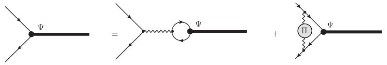
Figure 1: Feynman diagrams representing BSE. Thin solid lines represent KS state propagators, thick solid lines are excitons, zigzag lines – Coulomb potential; ${\Pi}$ is the polarization insertion, Eq. (10).

In our DFT simulations we have used hybrid Heyd-Scuseria-Ernzerhof (HSE06) exchange correlation functional Vydrov et al. (2006); Heyd et al. (2006), which has been successful in reproducing electronic gaps in various semiconductor nanostructures (e.g., Kümmel and Kronik (2008); Govoni and Galli (2015)). (See, however, Jain et al. (2011).) So, here using the HSE06 functional is to substitute for $GW$ corrections to the KS energies, i.e., for the first step in the standard three-step procedure Hybertsen and Louie (1986); Rohlfing and Louie (2000). Therefore, single-particle energy levels and wave functions are approximated by the KS $\epsilon_{i}$ and $\phi_{i}({\bf x})$ from the HSE06 DFT output. While $GW$ technique would improve accuracy of our calculations, it is unlikely to alter our results and conclusions qualitatively.

Now one is to apply standard perturbative many-body quantum mechanics techniques (e.g., Abrikosov et al. (1963); Fetter and Walecka (1971)) to compute the SF decay rates, i.e., exciton-to-bi-exciton, bi-exciton-to-exciton rates with the two triplet excitons in the total spin-zero state, working to the second order in the screened Coulomb interaction.

As noted above, phonon-meditated electron energy relaxation is an important process competing with MEG. A suitable approach to describe time-evolution of a photo-excited nanosystem is the Boltzmann transport equation which includes phonon emission/absorption terms together with the terms describing exciton-to-bi-exciton decay and recombination, along with the charge and energy transfer contributions, etc. This challenging task is work in progress. In this work electron-phonon interaction effects are only included by adding small imaginary parts to the KS energies $\epsilon_{i}\rightarrow\epsilon_{i}-i\gamma_{i}$, which results in the non-zero line-widths in the expressions below. In this work all $\gamma$ will be set to 0.025 eV corresponding to room temperature.

The KS orbital Fourier transformation conventions used in this work are

$$\phi_{i}({\bf k})=\frac{1}{\sqrt{V}}\int_{V}{\rm d}{\bf x}~{}\phi_{i}({\bf x}){\rm e}^{-i{\bf k}\cdot{\bf x}},~{}\phi_{i}({\bf x})=\frac{1}{\sqrt{V}}\sum_{{\bf k}}\phi_{i}({\bf k}){\rm e}^{i{\bf k}\cdot{\bf x}},$$

$${\bf k}=2\pi\left(\frac{n_{x}}{L_{x}},\frac{n_{y}}{L_{y}},\frac{n_{z}}{L_{z}}\right),~{}n_{x},n_{y},n_{z}=0,\pm 1,\pm 2,...$$ (11)

with $V=L_{x}L_{y}L_{z}$ being the simulation cell volume.

II.2 Medium Screening Approximation

For completeness, let us outline the main idea of the simplified treatment of medium screening used in this work Kryjevski and Kilin (2016); Kryjevski et al. (2016). The standard random phase approximation (RPA) Coulomb potential is

$${\rm W}(\omega,{\bf k},{\bf p})=\frac{4\pi e^{2}}{V}\left[k^{2}\delta_{{\bf k},-{\bf p}}-\Pi(\omega,{\bf k},{\bf p})\right]^{-1}.$$ (12)

In the static limit $\Pi(\omega,{\bf k},{\bf p})\simeq\Pi(\omega=0,{\bf k},{\bf p}).$ Evaluating ${\rm W}(0,{\bf k},{\bf p})$ requires matrix inversion which can severely limit applicability of the MBPT techniques Deslippe et al. (2012); Wilson et al. (2009). (See Govoni and Galli (2015) for recent advances.) In order to be able to simulate nanosystems of interest one is forced to sacrifice some accuracy. With this in mind, a significant technical simplification is to retain only the diagonal matrix elements in $\Pi(0,{\bf k},{\bf p}),$ i.e., to approximate $\Pi(0,{\bf k},{\bf p})\simeq\Pi(0,-{\bf k},{\bf k})\delta_{{\bf k},-{\bf p}}$ as implemented in Eqs. (8,17). In the position space this corresponds to $\Pi(0,{\bf x},{\bf x^{{}^{\prime}}})\simeq\Pi(0,{\bf x}-{\bf x^{{}^{\prime}}}),$ i.e., to approximating the system as a uniform medium. One rationale for this approximation is that in quasi one-dimensional systems, such as CNTs, one can expect $\Pi({\bf x},{\bf x^{{}^{\prime}}})\simeq\Pi(z-z^{{}^{\prime}}),$ where $z,z^{{}^{\prime}}$ are the axial positions.

Previously, we have checked quality of our computational approach including this screening approximation for chiral SWCNTs Kryjevski et al. (2016). We have computed low-energy absorption spectra for (6,2) and (10,5) SWCNTs and found that our predictions for $E_{11}$ and $E_{22}$ – the energies of the first two absorption peaks corresponding to transitions between the van Hove peaks in the CNT density of states – reproduce results of Weisman and Bachillo Weisman and Bachilo (2003) within 5 - 13 % error. Additionally, we have simulated SWCNT (6,5) and found $E_{11}=1.1~{}eV,~{}E_{22}=2.05~{}eV$ vs. $E_{11}=1.27~{}eV~{}eV,~{}E_{22}=2.19~{}eV$ from Weisman and Bachilo (2003). This suggests that our approach is adequate for the semi-quantitative description of these systems. Accuracy could be improved by using full interaction ${\rm W}(0,{\bf k},{\bf p}),$ or ${\rm W}(\omega,{\bf k},{\bf p})$, and GW, which would be much more computationally expensive. However, it would not change the overall conclusions of this work.

II.3 Expressions for the Rates

Within our approximations exciton-to-bi-exciton decay rate from the impact ionization process is given by

$${\rm R}_{1{\rightarrow}2}=-2{\rm Im}\Sigma_{\gamma}(\omega_{\gamma}),$$ (13)

where $\Sigma_{\gamma}(\omega)$ are the exciton-to-bi-exciton decay contributions to the self-energy function of the exciton state $\gamma$ with energy $E^{\gamma}=\hbar\omega_{\gamma}.$ The relevant self-energy Feynman diagrams are shown in Fig. 2.

For completeness, let us quote the expressions for the all-singlet exciton-to-bi-exciton rates Kryjevski et al. (2016)

$$R_{1{\to}2}(\omega_{\gamma}) = R^{p}+R^{h}+{\tilde{R}}^{p}+{\tilde{R}}^{h},$$

$$R^{p}(\omega_{\gamma}) = 2\frac{2\pi}{\hbar^{2}}\sum_{\alpha\beta}\delta(\omega_{\gamma}-\omega_{\alpha}-\omega_{\beta})\left\lvert\sum_{ijkln}W_{{jlnk}}\theta_{l}\theta_{-n}(\Psi_{ln}^{\beta}){}^{*}\theta_{i}\theta_{-j}\theta_{-k}\Psi_{{ij}}^{\gamma}\left(\Psi_{{ik}}^{\alpha}\right){}^{*}\right\rvert^{2},$$

$$R^{h}(\omega_{\gamma}) = 2\frac{2\pi}{\hbar^{2}}\sum_{\alpha\beta}\delta(\omega_{\gamma}-\omega_{\alpha}-\omega_{\beta})\left\lvert\sum_{ijkln}W_{{jlnk}}\theta_{-l}\theta_{n}\Psi_{{nl}}^{\beta}\theta_{-i}\theta_{j}\theta_{k}(\Psi_{{ji}}^{\gamma}){}^{*}\Psi_{{ki}}^{\alpha}\right\rvert^{2}.$$ (14)

The expressions for ${\tilde{R}}^{h}$ and ${\tilde{R}}^{p}$ are the same as the ones for $R^{h},~{}R^{p}$ with $W_{jlnk}$ replaced by $W_{jlkn}$ and divided by 2.

A spin-singlet state composed of two noninteracting spin-one excitons is (cf. Eq. 5 of Berkelbach et al. (2013))

$$|{\alpha\beta}\rangle_{TT;0} = \frac{1}{\sqrt{3}}\left({\rm B}_{1}^{\alpha\dagger}{\rm B}_{-1}^{\beta\dagger}-{\rm B}_{0}^{\alpha\dagger}{\rm B}_{0}^{\beta\dagger}+{\rm B}_{-1}^{\alpha\dagger}{\rm B}_{1}^{\beta\dagger}\right)|{g.s.}\rangle=$$

$$= \sum_{e,h,e^{{}^{\prime}},h^{{}^{\prime}}}\sum_{\mu,\nu,\lambda,\sigma}{\rm T}^{\mu\nu\lambda\sigma}{\rm\Phi}^{\alpha}_{eh}{\rm\Phi}^{\beta}_{e^{{}^{\prime}}h^{{}^{\prime}}}a^{\dagger}_{e\mu}a_{h\nu}a^{\dagger}_{e^{{}^{\prime}}\lambda}a_{h^{{}^{\prime}}\sigma}|{g.s.}\rangle,$$

$${\rm T}^{\mu\nu\lambda\sigma} = -\frac{1}{\sqrt{3}}\left(\delta_{\mu\sigma}\delta_{\nu\lambda}-\frac{1}{2}\delta_{\mu\nu}\delta_{\lambda\sigma}\right).$$ (15)

The expressions for the singlet fission rate, i.e., the rate for the singlet-to-two-triplets process, are

$$R^{SF}_{1{\to}2}(\omega_{\gamma}) = {\rm R}^{p}+{\rm R}^{h},$$

$${\rm R}^{p}(\omega_{\gamma}) = \frac{2\pi}{\hbar^{2}}\frac{3}{2}\sum_{\alpha\beta}\delta(\omega_{\gamma}-\omega_{1,\alpha}-\omega_{1,\beta})\left\lvert\sum_{ijkln}W_{{jlkn}}\theta_{l}\theta_{-n}(\Phi_{ln}^{\beta}){}^{*}\theta_{i}\theta_{-j}\theta_{-k}\Psi_{{ij}}^{\gamma}\left(\Phi_{{ik}}^{\alpha}\right){}^{*}\right\rvert^{2},$$

$${\rm R}^{h}(\omega_{\gamma}) = \frac{2\pi}{\hbar^{2}}\frac{3}{2}\sum_{\alpha\beta}\delta(\omega_{\gamma}-\omega_{1,\alpha}-\omega_{1,\beta})\left\lvert\sum_{ijkln}W_{{jlkn}}\theta_{-l}\theta_{n}\Phi_{{nl}}^{\beta}\theta_{-i}\theta_{j}\theta_{k}(\Psi_{{ji}}^{\gamma}){}^{*}\Phi_{{ki}}^{\alpha}\right\rvert^{2},$$ (16)

where ${\cal E}^{\gamma}=\hbar\omega_{1,\gamma}.$ In the above

$$W_{jlnk} = \sum_{{\bf q}\neq 0}\frac{4\pi e^{2}}{V}\frac{{{\rho}}_{kj}^{*}({\bf q}){{\rho}}_{ln}({\bf q})}{\left(q^{2}-\Pi(0,-{\bf q},{\bf q})\right)}$$ (17)

is the (approximate) screened Coulomb matrix element, and

$$\delta(x)=\frac{1}{\pi}\frac{\gamma}{x^{2}+\gamma^{2}},$$ (18)

the Lorentzian representation of the $\delta$-function. Only the direct channel diagram (Fig. 2, on the right) contributes to SF.

In the above expressions only the terms leading in the ratio of the typical exciton binding energy to the HO-LU gap $\epsilon_{binding}/E_{g}<1$ are shown, for brevity.

The rate as a function of energy is given by averaging over the initial exciton states within given energy range with the $\gamma=0.025~{}eV$ resolution, i.e.,

$$R(\epsilon)=\frac{1}{N(\epsilon)}\sum_{\alpha}R(E^{\alpha}),$$ (19)

where the sum is over the exciton states within the $(\epsilon,\epsilon+\gamma)$ energy range, $N(\epsilon)$ is the number of such states.

The above expressions have the overall structure of the Fermi Golden Rule. The bi-exciton-to-exciton rate expressions are given by similar expressions with the initial and final states reversed.

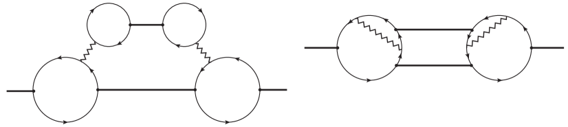
Figure 2: Exciton self-energy Feynman diagrams for the exciton$\to$bi-exciton process. Thin solid lines stand for the KS state propagators, thick solid lines depict excitons, zigzag lines – screened Coulomb potential. The diagrams on the left and the right correspond to the exchange and direct channels, respectively. Not shown for brevity are the similar diagrams with all the Fermion arrows reversed. Only the direct channel diagram contributes to SF. For SF final bi-exciton state is understood to be the singlet.

III Computational Details

The optimized geometries and KS orbitals and KS energy eigenvalues of the chiral SWCNTs studied here have been obtained using the ab initio total energy and molecular dynamics program VASP (Vienna ab initio simulation program) with the hybrid Heyd-Scuseria-Ernzerhof (HSE06) exchange correlation functional Vydrov et al. (2006); Heyd et al. (2006) using the projector augmented-wave (PAW) pseudopotentials Blöchl (1994); Kresse and Joubert (1999).

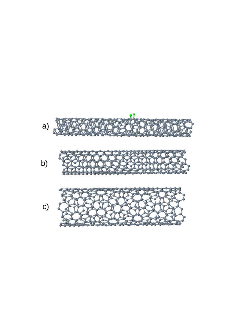
Figure 3: Atomistic models of chiral SWCNTs. Shown in a) is (6,2) with two chlorine atoms adsorbed to the surface in a para configuration. In order to keep the doping concentration low three unit cells have been included in the simulations. In b) is SWCNT (6,5). Only one unit cell is included due to computational cost restrictions. In c) is (10,5) with three unit cells.

Using conjugated gradient method for ion position relaxation the structures were relaxed until residual forces on the ions were no greater than $0.05~{}eV/\AA.$ The momentum cutoff defined by

$$\frac{\hbar^{2}{k}^{2}}{2m}\leq{\cal E}_{max},$$ (20)

where $m$ is the electron mass, was set to ${\cal E}_{max}=400~{}eV.$ The number of KS orbitals included in the simulations which regulated energy cutoff were chosen so that $\epsilon_{i_{max}}-\epsilon_{HO}\simeq\epsilon_{LU}-\epsilon_{i_{min}}\geq 3~{}eV,$ where $i_{max},~{}i_{min}$ are the highest and the lowest KS labels included in simulations.

SWCNT atomistic models were placed in various finite volume simulation boxes with periodic boundary conditions where in the axial direction the length of the box has been chosen to accommodate an integer number of unit cells, while in the other two directions the SWCNTs have been kept separated by about $1~{}nm$ of vacuum surface-to-surface thus excluding spurious interactions between their periodic images.

Previously, we have found reasonably small (about 10%) variation in the single particle energies over the Brillouin zone when three unit cells were included in the DFT simulations Kryjevski et al. (2016). So, simulations have been done including three unit cells of (6,2) and (10,5) SWCNTs at the $\Gamma$ point. So, in our approximation lattice momenta of the KS states, which are suppressed by the reduced Brillouin zone size, have been neglected. For (6,5) SWCNT due to high computational cost only one unit cell was included. But as mentioned above, simulation based on this size-reduced model reproduced the absorption spectrum features with the same accuracy as other SWCNTs. (See Table I.)

The rationale for including more unit cells instead of standard sampling of the Brillouin zone by including more $K$-points in the DFT simulations is that surfaces of these SWCNTs are to be functionalized. Inclusion of several unit cells allows us to keep the concentration of surface dopants reasonably low. So, here we have simulated (6,2) SWCNT doped with chlorine, where two $Cl$ atoms are attached to the same carbon ring in the para configuration, which has been found to be the preferred arrangement

The atomistic models of the optimized nanotubes are shown in Fig. (3). In this work all the DFT simulations have been done in a vacuum which should be adequate to describe properties of these SWCNTs dispersed in a non-polar solvent.

IV Results and Discussion

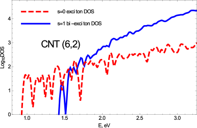
(a)	(b)
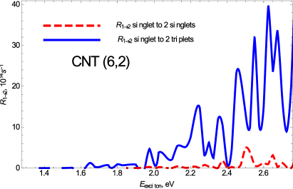
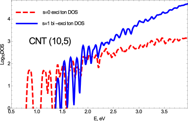
(c)	(d)
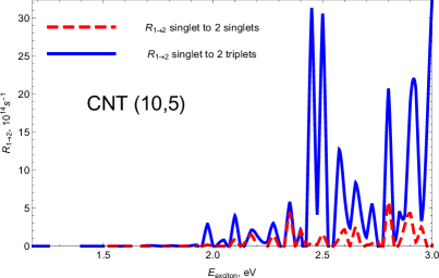
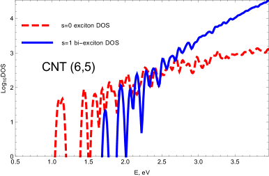
(e)	(f)

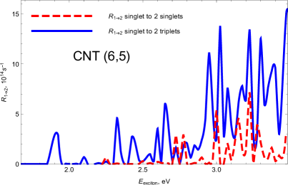
Figure 4: Singlet exciton and triplet biexciton densities of states (DOS) and the MEG $R_{1\to 2}$ rates, all-singlet and SF, for the (6,2) ((a) and (b)), (10,5) ((c) and (d)) and (6,5) ((e) and (f)) CNTs. The rates for (6,2) and (10,5) are from Kryjevski et al. (2016) and shown here for comparison. (Color on-line only.)

The main results are shown in Table I and in Figs. (4), (5). We have found (see Table I) that in all cases the lowest triplet exciton energy is red-shifted compared to the singlet, which is as expected since the repulsive exchange contribution to the BSE kernel is absent for the triplets Tretiak (2007). As a result, the energy threshold for SF is somewhat lower compared to the all-singlet MEG. The SF and all-singlet MEG rates for pristine (6,2), (10,5) and (6,5) SWCNTs are shown in Fig. (4). Shown here for comparison are the all-singlet rates for (6,2) and (10,5) are from Kryjevski et al. (2016).

$(6,2)$ $(6,2)+Cl_{2}$ $(6,5)$ $(10,5)$ $E_{g},~{}eV$ 1.33 0.96 1.22 0.91 $E_{g}^{BSE}~{}s=0,~{}eV$ 0.98 0.74 1.09 0.835 $E_{g}^{BSE}~{}s=1,~{}eV$ 0.73 0.27 0.86 0.71

Table 1: $E_{g}\equiv\epsilon_{LU}-\epsilon_{HO}$, is the HO-LU gap, $E^{BSE}_{g}$ is the minimal exciton energy from BSE for the singlets ($s=0$) and triplets ($s=1$).

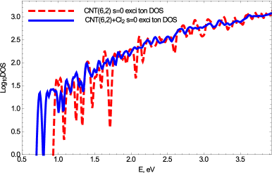
(a)	(b)
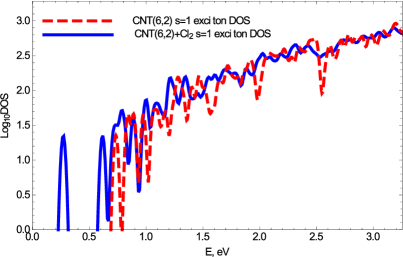
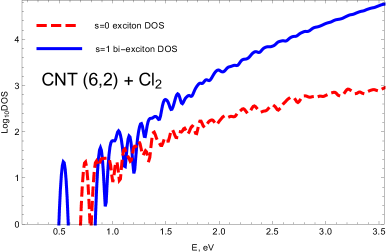
(c)	(d)

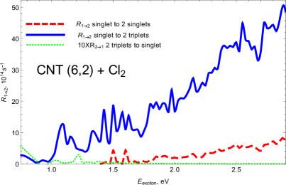
Figure 5: Exciton DOS and MEG rates for the pristine and doped (6,2) SWCNT. Shown in (a) are the singlet exciton DOSs for the pristine and $Cl$ doped (6,2) SWCNT; in (b) – the triplet exciton DOSs for the pristine and doped (6,2) SWCNT. Shown in (c) are the singlet exciton and triplet biexciton DOSs for the doped (6,2) SWCNT. In (d) are the MEG rates for the $Cl$ doped (6,2) SWCNT: dashed (red) line depicts the all-singlet exciton-to-biexciton rate $R_{1\to 2}$, solid (blue) line – the SF exciton-to-biexciton rate. The (green) dotted line corresponds to the biexciton-to-exciton rate $R_{2\to 1}$ of the $Cl$ doped (6,2) SWCNT. $R_{2\to 1}$ has been multiplied by 10 for better presentation . This recombination rate is the greatest of all the cases considered here. (Color on-line only.)

Our calculations predict that efficient MEG both in the SF and all-singlet channels is present in chiral SWCNTs within the solar spectrum range but its strength varies strongly with the excitation energy. This is clearly due to the highly non-uniform low-energy electronic spectrum in SWCNTs (see Fig. 4, (a), (c), (e)). The $R_{1\to 2}$ MEG rates reach $10^{14}-10^{15}~{}1/s$ (see Fig. 4, (b), (d), (f)). The recombination rates $R_{2\to 1}$ are suppressed for all energies with $R_{2\to 1}/R_{1\to 2}\leq 10^{-2}$ Kryjevski et al. (2016); they are not shown. In (6,2) the all-singlet MEG starts at the energy threshold $2\times E_{g}=1.95~{}eV,$ the SF – at $2.3\times E^{t}_{g}=1.7~{}eV,$ where $E^{t}_{g}$ is the minimal triplet exciton energy, but in (10,5) the all-singlet MEG becomes appreciable at about $2.4\times E_{g}=2.0~{}eV;$ the threshold for SF is $2.75\times E^{t}_{g}=1.95~{}eV.$ In (6,5) the all-singlet MEG starts at $2.1\times E_{g}=2.25~{}eV,$ SF – at $2.2\times E^{t}_{g}=1.9~{}eV,$

Shown in Fig. 5 are results for the (6,2) SWCNT with chlorine atoms attached to the surface as described in Section III. Complete discussion of the influence of this surface defect on the system’s optoelectronic properties will be presented elsewhere. As far as the MEG-related properties are concerned, we predict that doping significantly red-shifts exciton energy spectra, both singlet (Fig. 5, (a)) and triplet (Fig. 5, (b)). DOS for the initial and final MEG states are shown in Fig. 5, (c). In this case, SF MEG is energetically allowed even for the lowest singlet exciton. Shown in Fig. 5, (d) are the MEG rates for the $Cl$-decorated (6,2) SWCNT. The all-singlet MEG threshold is at about $2E_{g}=1.5~{}eV;$ the threshold for SF is $0.75~{}eV,$ which is the lowest singlet exciton energy. Importantly, both the all-singlet and SF MEG rates $R_{1\to 2}$ are much less oscillatory as a function of the exciton energy than the pristine case rates (cf. Fig. 4, (b) and 5, (d)). The recombination rate $R_{2\to 1}$ – which is the greatest of all the cases considered – is shown in Fig. 5, (d). Note that it is multiplied by 10 for better presentation.

In all cases we find that SF rates are greater in magnitude than the all-singlet rates. This is likely due to the aforementioned overall red-shift of the triplet biexciton spectrum compared to the singlet exciton energies. While the Coulomb interaction matrix elements between the electron/hole and trion states are similar in magnitude in both cases, for the same energy there are simply more available bi-exciton final states for the SF than for the all-singlet channel.

V Conclusions and Outlook

Working to the second order in the screened Coulomb interaction and including electron-hole bound state effects we have developed a DFT-based MBPT technique for SF which allows one to compute the exciton-to-bi-exciton and the inverse bi-exciton-to-exciton rates when the initial state is a high-energy singlet while the final state is a pair of non-interacting triplet excitons in spin-correlated state with the total spin zero. Then, this method was used to calculate MEG in the chiral SWCNTs, using (6,2), (6,5) and (10,5) as examples. Also, we have simulated (6,2) SWCNT with chlorine atoms adsorbed to the surface.

Our calculations suggest that chiral SWCNTs have efficient MEG within the solar spectrum range both for the all-singlet channel and SF with $R_{1\to 2}\sim 10^{14}-10^{15}~{}s^{-1}$ and with the recombination rates suppressed as $R_{2\to 1}/R_{1\to 2}\sim 10^{-2}.$ In the pristine SWCNTs the MEG rates vary strongly with the excitation energy. In contrast, our results for the $Cl$-decorated (6,2) SWCNT suggest that surface functionalization significantly alters low-energy spectrum in a SWCNT. As is typical for doping, the defect creates additional shallow electronic states, which improves MEG efficiency. In the doped case, $R_{1\to 2}$ is not only greater in magnitude, but also is a much smoother function of the excitation energy. An alternative way to increase efficiency of carrier multiplication is to use SWCNT mixtures of different chiralities.

As noted above, an investigation of MEG efficiency in a nanosystem should be comprehensive, i.e., carrier multiplication and biexciton recombination should be allowed to “compete” with other processes, such as phonon-mediated carrier relaxation, energy and charge transfer, etc. Stewart et al. (2013). The Kadanoff-Baym-Keldysh, or NEGF, technique is a suitable formalism to achieve this goal Lifshitz and Pitaevskii (1981); Dahnovsky (2011); Bernardi et al. (2014). Bi-exciton creation and recombination, both in the all-singlet and SF channels, phonon emission, recombination, energy and charge transfer and other effects are to be included in the transport equation describing time evolution of a weakly non-equilibrium photoexcited state.

As described above (see Section II), our calculations had to utilize several simplifying approximations. However, we have verified that our results for the absorption spectra are in reasonable agreement with experimental data with the error less then 13% for E₁₁ and E₂₂ excitonic bands for the (6,2), (6,5) and (10,5) nanotubes. This suggests overall applicability of our technique for these systems at least at the semi-quantitative level. Accuracy of our methods can be further improved in several ways. One natural improvement is to calculate $GW$ single particle energy corrections, which then can be easily incorporated in the rate expressions. It is likely to blue-shift the rate curves by a fraction of eV without significant changes to the shape. Another step is to use full RPA interaction ${\rm W}(0,{\bf k},{\bf p})$ rather than ${\rm W}(0,-{\bf k},{\bf k}).$ Also, in the impact ionization process the typical energy exchange exceeds the gap and, so, role of dynamical screening needs to be investigated. Going beyond second order in the screened Coulomb interaction would require keeping the wave function renormalization factor (see, e.g., Fetter and Walecka (1971)) in the exciton decay rate expressions in Eqs. (13), (16). However, none of these corrections are likely to change the main results of this work, while drastically increasing computational cost.

VI Acknowledgments

Authors acknowledge financial support from the NSF grant CHE-1413614. The authors acknowledge the use of computational resources at the Center for Computationally Assisted Science and Technology (CCAST) at North Dakota State University and the National Energy Research Scientific Computing Center (NERSC) allocation award 86678, supported by the Office of Science of the DOE under contract No. DE-AC02-05CH11231.

References

- Shockley and Queisser (1961) W. Shockley and H. Queisser, J. Appl. Phys. 32, 510 (1961).
- Ellingson et al. (2005a) R. J. Ellingson, M. C. Beard, J. C. Johnson, P. R. Yu, O. I. Micic, A. J. Nozik, A. Shabaev, and A. L. Efros, Nano Letters 5, 865 (2005a).
- Nozik (2002) A. J. Nozik, Physica E: Low-dimensional Systems and Nanostructures 14, 115 (2002).
- de Boer et al. (2013) W. D. A. M. de Boer, E. M. L. D. de Jong, D. Timmerman, T. Gregorkiewicz, H. Zhang, W. J. Buma, A. N. Poddubny, A. A. Prokofiev, and I. N. Yassievich, Phys. Rev. B 88, 155304 (2013).
- Stewart et al. (2013) J. Stewart, L. Padilha, W. Bae, W. Koh, J. Pietryga, and V. Klimov, The Journal of Physical Chemistry Letters 4, 2061 (2013).
- Bude and Hess (1992) J. Bude and K. Hess, Journal of Applied Physics 72, 3554 (1992).
- Jung et al. (1996) H. K. Jung, K. Taniguchi, and C. Hamaguchi, Journal of Applied Physics (1996).
- Harrison et al. (1999) D. Harrison, R. A. Abram, and S. Brand, AIP 85, 8186 (1999).
- Nozik (2001) A. Nozik, Annual Review of Physical Chemistry 52, 193 (2001).
- Ellingson et al. (2005b) R. Ellingson, M. Beard, J. Johnson, P. Yu, O. Micic, A. Nozik, A. Shabaev, and A. Efros, Nano Letters 5, 865 (2005b).
- McGuire et al. (2010) J. McGuire, M. Sykora, J. Joo, J. Pietryga, and V. Klimov, Nano Letters 10, 2049 (2010).
- Gabor (2013) N. M. Gabor, Accounts of Chemical Research 46, 1348 (2013).
- Semonin et al. (2011) O. Semonin, J. Luther, S. Choi, H.-Y. Chen, J. Gao, A. J. Nozik, and M. C. Beard, Science 334, 1530 (2011).
- Wang et al. (2010) S. Wang, M. Khafizov, X. Tu, M. Zheng, and T. Krauss, Nano Letters 10, 2381 (2010).
- Gabor et al. (2009) N. Gabor, Z. Zhong, K. Bosnick, J. Park, and P. McEuen, Science 325, 1367 (2009).
- Perebeinos and Avouris (2006) V. Perebeinos and P. Avouris, Phys. Rev. B 74, 121410 (2006).
- Konabe and Okada (2012) S. Konabe and S. Okada, Phys. Rev. Lett. 108, 227401 (2012).
- Velizhanin and Piryatinski (2011) K. Velizhanin and A. Piryatinski, Phys. Rev. Lett. 106, 207401 (2011).
- Velizhanin and Piryatinski (2012) K. A. Velizhanin and A. Piryatinski, Phys. Rev. B 86, 165319 (2012).
- Kilina et al. (2015) S. Kilina, D. Kilin, and S. Tretiak, Chemical Reviews 115, 5929 (2015).
- Kryjevski et al. (2016) A. Kryjevski, B. Gifford, S. Kilina, and D. Kilin, The Journal of Chemical Physics 145, 154112 (2016).
- Smith and Michl (2010) M. B. Smith and J. Michl, Chemical Reviews 110, 6891 (2010).
- Lee et al. (2013) J. Lee, P. Jadhav, P. D. Reusswig, S. R. Yost, N. J. Thompson, D. N. Congreve, E. Hontz, T. Van Voorhis, and M. A. Baldo, Accounts of Chemical Research 46, 1300 (2013).
- Tretiak (2007) S. Tretiak, Nano Letters 7, 2201 (2007).
- Wang et al. (2016) X. Wang, T. Garcia, S. Monaco, B. Schatschneider, and N. Marom, CrystEngComm 18, 7353 (2016).
- Stich et al. (2014) D. Stich, F. Spath, H. Kraus, A. Sperlich, V. Dyakonov, and T. Hertel, Nature Photonics 8, 139 (2014).
- Fetter and Walecka (1971) A. L. Fetter and J. Walecka, Quantum Theory of Many-Particle Systems (McGraw-Hill, New York, 1971).
- Mahan (1993) G. Mahan, Many-Particle Physics (Plenum, New York, N.Y., 1993), 2nd ed.
- Kryjevski and Kilin (2014) A. Kryjevski and D. Kilin, Molecular Physics 112, 430 (2014).
- Onida et al. (2002) G. Onida, L. Reining, and A. Rubio, Rev. Mod. Phys. 74, 601 (2002).
- Kümmel and Kronik (2008) S. Kümmel and L. Kronik, Rev. Mod. Phys. 80, 3 (2008).
- Rohlfing and Louie (2000) M. Rohlfing and S. Louie, Phys. Rev. B 62, 4927 (2000).
- Strinati (1984) G. Strinati, Phys. Rev. B 29, 5718 (1984).
- Berestetskii et al. (1979) V. Berestetskii, E. Lifshitz, and L. Pitaevskii, Quantum Electrodynamics (Oxford, U.K.: Pergamon Press, 1979).
- Beane et al. (2000) S. Beane, P. Bedaque, W. Haxton, D. Phillips, and M. Savage, Shifman, M. (ed.): At the frontier of particle physics 1, 133 (2000).
- Spataru et al. (2004) C. Spataru, S. Ismail-Beigi, L. Benedict, and S. Louie, Phys. Rev. Lett. 92, 077402 (2004).
- Perebeinos et al. (2004) V. Perebeinos, J. Tersoff, and P. Avouris, Phys. Rev. Lett. 92, 257402 (2004).
- Spataru et al. (2005) C. Spataru, S. Ismail-Beigi, R. Capaz, and S. Louie, Phys. Rev. Lett. 95, 247402 (2005).
- Öğüt et al. (2003) S. Öğüt, R. Burdick, Y. Saad, and J. Chelikowsky, Phys. Rev. Lett. 90, 127401 (2003).
- Benedict et al. (2003) L. Benedict, A. Puzder, A. Williamson, J. Grossman, G. Galli, J. Klepeis, J.-Y. Raty, and O. Pankratov, Phys. Rev. B 68, 085310 (2003).
- Wilson et al. (2009) H. Wilson, D. Lu, F. Gygi, and G. Galli, Phys. Rev. B 79, 245106 (2009).
- Rohlfing and Louie (1998) M. Rohlfing and S. G. Louie, Phys. Rev. Lett. 80, 3320 (1998).
- Vydrov et al. (2006) O. Vydrov, J. Heyd, A. Krukau, and G. Scuseria, The Journal of Chemical Physics 125, 074106 (2006).
- Heyd et al. (2006) J. Heyd, G. Scuseria, and M. Ernzerhof, The Journal of Chemical Physics 124, 219906 (2006).
- Govoni and Galli (2015) M. Govoni and G. Galli, Journal of Chemical Theory and Computation 11, 2680 (2015).
- Jain et al. (2011) M. Jain, J. R. Chelikowsky, and S. G. Louie, Phys. Rev. Lett. 107, 216806 (2011).
- Hybertsen and Louie (1986) M. Hybertsen and S. Louie, Phys. Rev. B 34, 5390 (1986).
- Abrikosov et al. (1963) A. A. Abrikosov, L. Gorkov, and I. E. Dzyaloshinski, Methods of Quantum Field Theory in Statistical Physics (Prentice-Hall, Englewood Cliffs, NJ, 1963).
- Kryjevski and Kilin (2016) A. Kryjevski and D. Kilin, Molecular Physics 114, 365 (2016).
- Deslippe et al. (2012) J. Deslippe, G. Samsonidze, D. Strubbe, M. Jain, M. Cohen, and S. Louie, Computer Physics Communications 183, 1269 (2012).
- Weisman and Bachilo (2003) R. B. Weisman and S. Bachilo, Nano Letters 3, 1235 (2003).
- Berkelbach et al. (2013) T. C. Berkelbach, M. S. Hybertsen, and D. R. Reichman, The Journal of Chemical Physics 138, 114102 (2013).
- Blöchl (1994) P. E. Blöchl, Phys. Rev. B 50, 17953 (1994).
- Kresse and Joubert (1999) G. Kresse and D. Joubert, Phys. Rev. B 59, 1758 (1999).
- Lifshitz and Pitaevskii (1981) E. M. Lifshitz and L. P. Pitaevskii, Physical Kinetics (Pergamon Press, New York, 1981), 1st ed.
- Dahnovsky (2011) Y. Dahnovsky, Phys. Rev. B 83, 165306 (2011).
- Bernardi et al. (2014) M. Bernardi, D. Vigil-Fowler, J. Lischner, J. B. Neaton, and S. G. Louie, Phys. Rev. Lett. 112, 257402 (2014).