Controlling the sign problem in Finite Density Quantum Field Theory

Abstract

Quantum field theories at finite matter densities generically possess a partition function that is exponentially suppressed with the volume compared to that of the phase quenched analogue. The smallness arises from an almost uniform distribution for the phase of the fermion determinant. Large cancellations upon integration is the origin of a poor signal to noise ratio. We study three alternatives for this integration: the Gaussian approximation, the “telegraphic” approximation, and a novel expansion in terms of theory-dependent moments and universal coefficients. We have tested the methods for QCD at finite densities of heavy quarks. We find that for two of the approximations the results are extremely close - if not identical - to the full answer in the strong sign problem regime.

1 Introduction

The sign problem is known to be one the most important challenges of modern physics. In theoretical particle physics, it prevents us from simulating finite-density QCD with standard Monte-Carlo methods. Hence most of the QCD phase diagram cannot be explored by first-principle techniques, such as lattice QCD. Many reviews can be found, see for example Fukushima:2010bq ; deForcrand:2010ys ; Gupta:2011ma ; Levkova:2012jd ; Aarts:2013lcm ; Gattringer:2014nxa ; Sexty:2014dxa ; Borsanyi:2015axp ; Langfeld:2016kty .

Dropping the phase factor of the quark determinant $\exp\{i\phi\}$ from the functional integral results in a theory, say with partition function $Z_{PQ}$, that is accessible by standard importance sampling Monte-Carlo simulations. Very early on, it became clear that $Z_{PQ}$ and the partition function of the full theory $Z$ are only comparable for the smallest values of the chemical potential $\mu$ Troyer:2004ge . The deviation is quantified by the so-called phase factor expectation value

$$\langle\mathrm{e}^{i\phi}\rangle_{PQ}\;=\;Z(\mu)/Z_{PQ}(\mu)\;\propto\;\mathrm{e}^{-\Delta f\,V}\;,$$ (1)

where $\Delta f$ is the free energy difference between the full and the phase quenched theory and $V$ is the volume (see e.g. Troyer:2004ge ). The knowledge of this phase factor would give access to the partition function $Z(\mu)$ (we assume that $Z_{PQ}(\mu)$ has been obtained by standard methods). In this work, we study its expectation value, $\langle\mathrm{e}^{i\phi}\rangle_{PQ}$: it is a very small number, generically very hard to measure due to the statistical noise, which only decreases proportionally to the square root of the number of Monte-Carlo configurations. Our approach is based on the density-of-states method and in particular on the LLR formulation Langfeld:2012ah ; Langfeld:2015fua , which is ideally suited to calculate probability distributions of observables: it features an exponential error suppression Langfeld:2015fua which can result in an unprecedented precision for the observable (see e.g. for an early example Langfeld:2013xbf ). It is based upon a non-Markovian Random Walk, which immediately provides two main advantages: it bears the potential to overcome the critical slowing down for theories close to a first order phase transition Lucini:2016fid ; Langfeld:2016kty , and it is not restricted to theories with a positive probabilistic weight for Monte-Carlo configurations. In fact, the method has been successfully applied to the $Z_{3}$ theory at finite densities Langfeld:2014nta and QCD at finite densities of heavy quarks Garron:2016noc . In both cases, the probability density $\rho(\phi)$ of the phase $\phi$ has been obtained to very high precision. The phase factor expectation value is then given by

$$\langle\mathrm{e}^{i\phi}\rangle_{PQ}\;=\;\frac{\int d\phi\;\rho(\phi)\;\exp\{i\phi\}}{\int d\phi\;\rho(\phi)}.$$ (2)

Despite of high quality numerical result for $\rho(\phi)$, the challenge remains to extract a very small signal from the above Fourier transform. An approach, put forward in Langfeld:2014nta ; Garron:2016noc , is to first represent the numerical data for $\ln\rho(\phi)$ by a fit function and then to calculate the Fourier transform of the fit function (semi-)analytically. The method produces reliable results if all the numerical data are well represented by the fit function with a small number of fit parameters Langfeld:2014nta ; Garron:2016noc . With the advent of high precision data for $\rho(\phi)$, the main obstacle for gaining access to quantum field theories at finite densities is the above Fourier transform. The method used in Langfeld:2014nta ; Garron:2016noc hinges on the fact that a fit function which faithfully represents the data could be found. This might not be generically the case.

In this paper, we propose three alternatives to this direct method. In Section 3 we present the first approach, called Gaussian approximation. No fitting procedure is required, instead the phase factor is computed directly from the data. Within this framework, the integral in the numerator of (2) is known analytically. The second approximation, presented in Section 4 is what we call the “telegraphic” approximation. This approach can be implemented either on the fit function or directly on the data (although it might require new simulations). The integral is replaced by a simple difference. In Section 5, we introduce a third method, the “Advanced Moment expansion”, which can be seen as a variant of a cumulant expansion Ejiri:2007ga ; Nakagawa:2011eu ; Saito:2012nt ; Saito:2013vja . It is a systematic expansion in the deviation from the uniform distribution and as such is expected to work better in the strong sign-problem regime. We will provide evidence that the universal coefficients decrease exponentially with increasing order, providing a rapid convergence if the moments are bounded. Although the convergence is faster in the strong sign-problem regime, for the phase factor expectation value we find an excellent agreement already at the third order of the expansion, regardless of the strength of the sign problem. In this case we still rely on a fitting procedure for the density of states. However the direct computation of the Fourier transform (2) is not needed, only the elementary moments are required. Before going through the details of these methods, we present the framework and the numerical details of our simulations in the next section. Our conclusions are presented in 6

2 Generalities and Framework

2.1 Full theory and phase quenching

We consider a generic theory with a partition function

$$Z\;=\;\int{\cal D}U_{\mu}\;\exp\{\beta\,S_{\mathrm{YM}}[U]\}\;\hbox{Det}M[U]\;,$$ (3)

and with a complex “matter” determinant:

$$\hbox{Det}M[U]=|\hbox{Det}M[U]|\;\exp\{i\phi[U]\}\;,\;\;\;\phi\in]-\pi,\pi]\;.$$ (4)

With the help of the density of states

$$\rho(s)\;=\;\int{\cal D}U_{\mu}\;\exp\{\beta\,S_{\mathrm{YM}}[U]\}|\hbox{Det}M[U]|\delta(s-\phi[U])\;,$$ (5)

the partition function can then be recovered by a 1-dimensional Fourier transform:

$$Z\;=\;\int ds\;\rho(s)\;\exp\{is\}\;=\;\int ds\;\rho(s)\;\cos(s)\;.$$ (6)

We also introduce the so-called phase quenched counter part by

$$Z_{PQ} = \int{\cal D}U_{\mu}\;\exp\{\beta\,S_{\mathrm{YM}}[U]\}\;|\hbox{Det}M[U]|\;,$$ (7)

$$= \;\int ds\;\rho(s)\;.$$ (8)

The expectation values of an observable $A$ in the full and in the phase quenched theory are given as usual by

$$\langle A\rangle = \frac{1}{Z}\int{\cal D}U_{\mu}\;A\exp\{\beta\,S_{\mathrm{YM}}[U]\}\hbox{Det}M[U]\;,$$ (9)

$$\langle A\rangle_{PQ} = \frac{1}{Z_{PQ}}\int{\cal D}U_{\mu}\;A\exp\{\beta\,S_{\mathrm{YM}}[U]\}|\hbox{Det}M[U]|\;,$$

implying the well-known relations

$$\langle A\rangle=\frac{\langle A\mathrm{e}^{i\phi}\rangle_{PQ}}{\langle\mathrm{e}^{i\phi}\rangle_{PQ}}\;\hbox to28.45274pt{\hfill}Z\;=\;Z_{PQ}\;\langle\mathrm{e}^{i\phi}\rangle_{PQ}\;.$$ (11)

In terms of the density, the phase factor expectation value is given by (2).

2.2 Extensive density of states

For theories for which the imaginary part arises from a local action an extensive phase $x\in]-\infty,\infty[$ can be defined as the sum of the local phases. This has been e.g. the case for the finite density $Z_{3}$ and for heavy dense QCD Langfeld:2014nta ; Garron:2016noc . For fermionic theories with the phase $\phi[U]$ arising from the (non-local) quark determinant, an extensive phase can still be defined as pointed out in Greensite:2013gya :

$$x[U] = \hbox{Im ln}\,(\hbox{Det}M)$$ (12)

$$= \int_{0}^{\mu/T}\hbox{Im}\,\left[\frac{\partial(\hbox{ln}\,Det)M)}{\partial\mu/T}\right]_{\mu=\bar{\mu}}\;d\left(\frac{\bar{\mu}}{T}\right)$$

$$= \int_{0}^{\mu/T}\hbox{Im}\,\hbox{tr}\left[M^{-1}\frac{\partial M)}{\partial\mu/T}\right]_{\mu=\bar{\mu}}\;d\left(\frac{\bar{\mu}}{T}\right)$$

The definition of an extensive phase factor has proven to be important to achieve the precision needed for the Fourier transform. If $\rho_{E}(x)$ denotes the corresponding probability distribution, the phase factor expectation value in (2) is obtained by

$$\langle\mathrm{e}^{i\phi}\rangle_{PQ}=\frac{1}{Z_{PQ}}\int_{-\infty}^{+\infty}dx\;\rho_{E}(x)\cos(x)\;.$$ (13)

The density of states $\rho(s)$ can be easily recovered from the extended density $\rho_{E}(x)$. To see this, we subtract from $x$ a multiple of $2\pi$ until $s\in[-\pi,\pi[$, $s=x-2\pi\,n$, $n\in\mathbb{Z}$, and split the integration domain in intervals of size $2\pi$:

$$\langle\mathrm{e}^{i\phi}\rangle_{PQ} = \frac{1}{Z_{PQ}}\sum_{n\in{\mathbb{Z}}}\int_{-\pi}^{\pi}ds\;\rho_{E}(s+2n\pi)\cos(s)\;,$$ (14)

$$= \frac{1}{Z_{PQ}}\int_{-\pi}^{\pi}ds\,\rho(s)\,\cos(s)\;,$$

and identify:

$$\rho(s)\equiv\sum_{n\in{\mathbb{Z}}}\rho_{E}(s+2\pi n)\;.$$ (15)

Also note that

$$Z_{PQ}\;=\;\int_{-\pi}^{\pi}ds\;\rho(s)\;=\;\int_{-\infty}^{\infty}dx\;\rho_{E}(x)\;.$$

2.3 Volume dependence of the density

We here consider the class of theories for which the phase of the Gibbs factor is proportional to the chemical potential $\mu$ and for which this is the only $\mu$ dependence. Scalar theories do not fall into this class since the real part of the action also acquires a $\mu$ dependence, but fermion theories in the ab initio continuum formulation might fall into this class. For these theories, let us study the dependence of $\rho_{E}(s)$ on the physical volume $V$. We make explicit the $\mu$ dependence of the phase factor expectation value and point out that the partition function is positive for all $\mu$:

$$z(\mu)\;=\;\langle\mathrm{e}^{i\,\mu\,\phi}\rangle_{PQ}\;\geq\;0\;.$$ (16)

Note that we have $z(0)=1$ and that we will assume that

$$\langle\mathrm{e}^{-i\,\mu\,\phi}\rangle_{PQ}\;=\;\langle\mathrm{e}^{i\,\mu\,\phi}\rangle_{PQ}\;\;\Rightarrow\;\;z(-\mu)=z(\mu)\;.$$ (17)

Note that since $z(\mu)$ is obtained by a Fourier transform of $\rho$, see (2), the density of states can be recovered from $z(\mu)$ by the inverse Fourier transform (up to a normalisation constant $Z_{PQ}\geq 0$)

$$\rho_{E}(s)\;=\;Z_{PQ}\;\int\frac{d\mu}{2\pi}\;z(\mu)\,\mathrm{e}^{-is\mu}\;.$$ (18)

As argued in Greensite:2013gya , $z(\mu)$ can be viewed as a partition function with free energy density $f(\mu)$ (a necessary condition is that $z(\mu)\geq 0$), leaving us with the volume dependence:

$$z(\mu) = \exp\{-f(\mu)\,V\}\;,$$ (19)

$$= \exp\{-[c_{1}\mu^{2}+c_{2}\mu^{4}+c_{3}\mu^{6}+\ldots]\;V\}\;,$$ (20)

where the coefficients $c_{k}$ are volume independent. Inserting (20) into (18), we find with an expansion in inverse powers of $V$:

$$\rho_{E}(s)=\mathrm{const.}\;\exp\left\{-a_{1}\,\frac{s^{2}}{V}-a_{2}\,\frac{s^{4}}{V^{3}}-a_{3}\,\frac{s^{6}}{V^{5}}+\ldots\right\}\;,$$ (21)

$$a_{1} = \frac{1}{4c_{1}}\;+\;{\cal O}(1/V),\;\;\;a_{2}\;=\;\frac{c_{2}}{16c_{1}^{4}}\;+\;{\cal O}(1/V)$$

$$a_{3} = -\frac{3c_{2}^{2}+c_{3}c_{2}}{c_{1}^{7}}\;+\;{\cal O}(1/V).$$

If we define a “scaling” variable by $x=s/\sqrt{V}$, the deviation from a Gaussian distribution decreases with increasing volume:

$$\rho_{E}(s)=\mathrm{const.}\;\exp\left\{-a_{1}\,x^{2}-a_{2}\,\frac{x^{4}}{V}-a_{3}\,\frac{x^{6}}{V^{2}}+\ldots\right\}\;.$$ (22)

2.4 Numerical details

We use the data obtained in our previous work Garron:2016noc but have also generated new simulations for reasons that we explain below. We summarise here the parameters used for the numerical simulations and the methods to obtain the density of states. The interested reader will find more details in the aforementioned reference. The lattice parameters are

$$\hbox{$8^{4}$ lattice},\;\;\beta=5.8,\;\;\kappa=0.12\;.$$

and we let the chemical potential $\mu$ vary between 1.0421 and 1.4321. We identified the “strong sign problem region” as being $1.1<\mu<1.4$. We for each value of $\mu$, we split the domain of the phase $s\in\left[0,s_{\rm max}\right]$ in $n_{\rm int}$ small interval of size $\delta_{s}$ and on each interval $k$, we compute the LLR coefficients $a_{k}$. In practise we choose $s_{\rm max}\sim 36$, $\delta_{s}=0.896$ and $n_{\rm int}=40$, except for a few values of the chemical potential, for which we need a better resolution. The corresponding values are reported in Table 1.

$\mu$	$\delta_{s}$	$n_{\rm nint}$
1.1821	0.29867	120
1.3721	0.4480	80
1.3921	0.4480	80
1.4121	0.4480	80

Table 1: Size and number of intervals for the LLR simulations. For the other values of $\mu$, we choose $\delta_{s}=0.896$ and $n_{\rm int}=40$.

We reconstruct the probability density function for discrete values of the phase $s_{k}=k\delta_{s}+\delta_{s}/2$, namely

$$\rho_{E}(s_{k})=\exp\left\{-\sum_{i=1}^{k-1}a_{i}\delta_{s}-a_{k}\delta_{s}/2\right\}\;.$$ (23)

In Garron:2016noc we performed a polynomial fit of $\ln(\rho_{E})$ and computed (13) by a semi-analytic integration (we refer to this method as “Exact”).

Although the fits are of very good quality and very stable, for three values of the chemical potential, we have also ran new simulations with $\delta_{s}=\pi/5$. As shown below, these new data allow us to compute $\rho(s)$ directly from the data (without relying on any fitting procedure) and will be very useful to check the methods presented here. We have implemented this technique for three different values of the chemical potential. This is illustrated in Figures 1,2 and 3, where we see that the different methods give compatible results.

Finally, we mention that we use around $1000$ configurations and that the statistical errors are estimated with the bootstrap method, using 500 samples. Naturally we have checked that the errors are stable with respect to the number of samples.

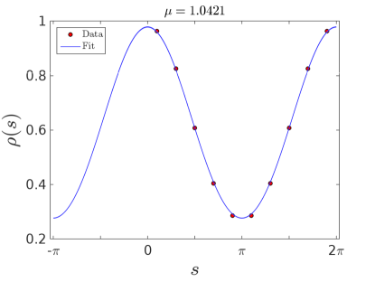
Figure 1: The density obtained directly from the data or from fitting the extensive density $\rho_{E}$, in the low density-region where the sign problem is weak.

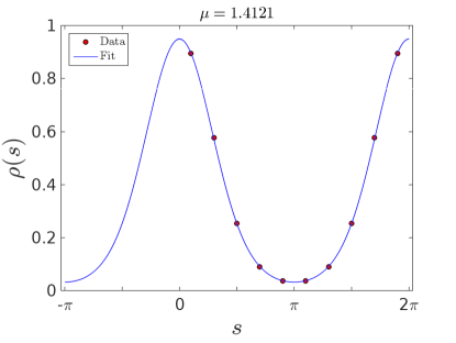
Figure 2: Same as Fig. 2 but with the density close to offset, again the sign problem is weak

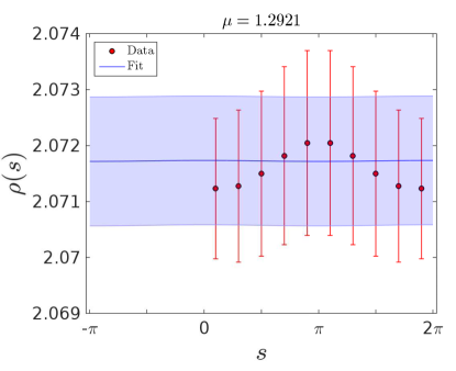
Figure 3: Same as previous figures but in the strong sign problem regime. The blue band corresponds to the $1-\sigma$ region obtained from the fit.

3 The Gaussian approximation

The smallness of $\langle\mathrm{e}^{i\phi}\rangle_{PQ}$ arises from large cancellations in (2). It was pointed out be Ejiri Ejiri:2007ga that these cancellations can be avoided by using cumulants of the phase factor:

$$\langle\mathrm{e}^{i\phi}\rangle_{PQ}\;=\;\exp\left[-\frac{1}{2}\langle\phi^{2}\rangle_{c}\,+\,\frac{1}{4!}\,\langle\phi^{4}\rangle_{c}-\,\ldots\right]\;.$$ (24)

In fact, numerical results suggest that the probability distribution is Gaussian to a good extent Ejiri:2007ga ; Ejiri:2012ng ; Ejiri:2012wp ; Ejiri:2013lia , which would imply that only the cumulant $\langle\phi^{2}\rangle_{c}$ is non-vanishing. It has been argued in Greensite:2013gya that higher cumulants are suppressed by factors of the volume $V$ and that, however, higher order cumulants are important for the medium and high range of chemical potentials. Throughout this paper, we define the Gaussian approximation as the approximation of the extended density of states by a normal distribution:

$$\rho_{E}(s)\approx\mathrm{const.}\;\exp\left\{-\epsilon\,s^{2}\right\}\;.$$ (25)

The phase factor expectation value (2) is then analytically obtained:

$$\langle\mathrm{e}^{i\phi}\rangle_{PQ}\;=\;\exp\left\{-\frac{1}{4\epsilon}\right\}\;.$$ (26)

We extract the parameter $\epsilon$ from the standard expectation value by

$$\langle s^{2}\rangle_{E}\;=\;\frac{1}{2\,\epsilon}\;\;\;\Rightarrow\;\;\;\langle\mathrm{e}^{i\phi}\rangle_{PQ}\;=\;\exp\left\{-\frac{1}{2}\langle s^{2}\rangle_{E}\right\},$$ (27)

where the subscript $E$ indicates that the expectation values are defined with respect to the extended density $\rho_{E}$. We test this approach for heavy-dense QCD with partition function (7). We find the expectation value in  (27) directly from the data: we take the density obtained through (23) and compute the expectation value $\langle s^{2}\rangle_{E}$ using a trapezoidal approximation. We obtain in this way an estimate for the phase factor expectation value (26) without invoking any fitting procedure. Our numerical findings are summarised in Figure 4. We find that the Gaussian approximation provides a surprisingly good approximation over the whole range of chemical potentials $\mu$. Even in the strong sign-problem regime at intermediate values $\mu$, the cancellations are well emulated and the approximate result only underestimates the true result by roughly a factor $2$.

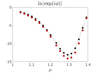
Figure 4: The phase factor expectation value in Gaussian approximation (red symbols) in comparison with the exact result (black) from Garron:2016noc .

4 The “telegraphic” approximation

4.1 Methodology

As can be seen in Figure 3, $\rho$ weakly depends on its arguments in the strong sign-problem regime and for large volumes. In this case, a Poisson re-summation of (15) should yield a rapidly converging series:

$$\rho(s) = \sum_{\nu\in\mathbb{Z}}b_{\nu}\;,$$ (28)

$$b_{\nu} = \int_{-\infty}^{\infty}dn\;\mathrm{e}^{2\pi i\,\nu\,n}\,\rho_{E}(s+2\pi n)$$

$$= \frac{1}{2\pi}\;\mathrm{e}^{-i\,\nu\,s}\;\int_{-\infty}^{\infty}dx\;\mathrm{e}^{i\,\nu\,x}\;\rho_{E}(x)\;.$$

The sum over $\nu$ in (28) becomes:

$$\rho(s) = c_{0}\;+\;\sum_{\nu=1}^{\infty}c_{\nu}\;\cos(\nu\,s)\;,$$ (29)

$$c_{0} = \frac{1}{2\pi}\int_{-\infty}^{\infty}dx\;\rho_{E}(x)\;,$$ (30)

$$c_{\nu} = \frac{1}{\pi}\int_{-\infty}^{\infty}dx\;\cos(\nu x)\;\rho_{E}(x)\;,\;\;\;\nu\geq 1.$$ (31)

Note that we find in view of (13)

$$c_{1}/c_{0}\;=\;2\;\langle\mathrm{e}^{i\phi}\rangle_{PQ}\;.$$ (32)

If the sum over $\nu$ is rapidly converging, we find approximately:

$$\rho(s)/c_{0}\;\approx\;1\;+\;2\;\langle\mathrm{e}^{i\phi}\rangle_{PQ}\;\cos(s)\;.$$ (33)

In the strong sign-problem regime, the amplitude of the cosine is very small, and therefore we see that $\rho(s)$ is almost a constant. Equation (33) then offers the possibility to extract the phase factor expectation value, i.e.,

$$\langle\mathrm{e}^{i\phi}\rangle_{PQ}\;\approx\;\frac{1}{4c_{0}}\Bigl{[}\rho(0)-\rho(\pi)\Bigr{]}\;.$$ (34)

Using (15), we therefore find:

$$\langle\mathrm{e}^{i\phi}\rangle_{PQ}\;\approx\;\frac{\pi}{2}\;\frac{\sum_{k\in\mathbb{Z}}(-1)^{k}\,\rho_{E}(k\pi)}{\int_{-\infty}^{\infty}dx\;\rho_{E}(x)}\;.$$ (35)

We call this the telegraphic approximation. It emerges by neglecting higher contributions $c_{\nu}$ of the Poisson sum. In order to get a feeling for the resulting systematic error, we adopt, for now only, the Gaussian approximation (25) and find:

$$\frac{c_{2}}{c_{1}}\;\approx\;\left[\exp\left(-\frac{1}{4\epsilon}\right)\right]^{3}.$$

This implies that the correction to $\rho(s)$ in (33) is of order:

$$\frac{c_{2}}{c_{0}}=\frac{c_{2}}{c_{1}}\frac{c_{1}}{c_{0}}\;=\;\approx\;2\,\left[\langle\mathrm{e}^{i\phi}\rangle_{PQ}\right]^{4}\;,$$

where we have used (26) and (32). At least in the strong sign-problem regime, for which $\langle\mathrm{e}^{i\phi}\rangle_{PQ}$ is very small, we expect the telegraphic approximation to work very well.

We finally point out that the telegraphic approximation can be improved in a systematic way. The order of the approximation is defined by the number of harmonics entering the density of states. E.g., in 3rd order we have:

$$\rho(s)/c_{0} \approx 1\;+\;2\;\langle\mathrm{e}^{i\phi}\rangle_{PQ}\;\cos(s)\;+\;c\;\cos(2s)$$

$$+ d\;\cos(3s)\;,$$

with the unknowns $\langle\mathrm{e}^{i\phi}\rangle_{PQ}$ and $c,d$. We generate three equations by evaluating $\rho(s)$ at $s=0,\,\pi/3,\,\pi$ and solve the linear set of equations for the unknowns. We are predominantly interested in the phase factor:

$$\langle\mathrm{e}^{i\phi}\rangle_{PQ} \approx -\frac{1}{2}\;+\;\frac{1}{4}\rho(0)/c_{0}\;+\;\frac{1}{3}\rho(\pi/3)/c_{0}$$

$$- \frac{1}{12}\;\rho(\pi)/c_{0}\;,$$

which can be easily converted to a discrete sum over discrete set of points of $\rho_{E}(s)$ using (15)  .

4.2 Numerical implementation

Again, we use Heavy-Dense QCD to test this approximation. Having in hands the density of state - either $\rho_{E}$ obtained from the fit or $\rho$ from the date through (15) - it is straightforward to implement numerically (35). If we take the results from the fit, we find that this approximation provide results extremely close to the “exact” ones: except for a few values of $\mu$ in the weak sign problem regime, the results (central value and variance) are actually indistinguishable. For example, for $\mu=1.0821$, we find

$$\ln\langle\mathrm{e}^{i\phi}\rangle_{PQ}^{\rm exact} = -1.992175\pm 2.910279\times 10^{-3}\;,$$ (38)

$$\ln\langle\mathrm{e}^{i\phi}\rangle_{PQ}^{\rm approx} = -1.992174\pm 2.910306\times 10^{-3}\;.$$ (39)

We show our results for the various $\mu$ in Table 2 and Figure 5.

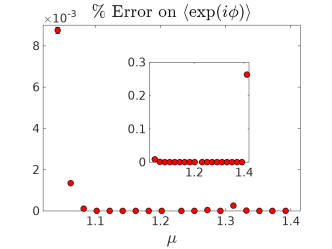
Figure 5: Relative difference (in percentage) on the phase factor expectation value between the telegraphic approximation (35) and the “exact” answer Garron:2016noc . Not visible in the plot is the point $\mu=1.4121$, for which the relative error is $0.3\%$

We have also implemented this approximation for our new simulations where $\delta_{s}=\pi/5$, such that we can compute $\rho(s)$ directly from the data (without relying on any fitting procedure). In that case we have $\rho(s)$ for $s=\pi/10,3\pi/10,\ldots$, but do not have $\rho(0)$ nor $\rho(\pi)$. Therefore we use a variant of (34):

$$\langle\mathrm{e}^{i\phi}\rangle_{PQ}\;\approx\;\frac{1}{4c_{0}\cos(\delta_{s}/2)}\Bigl{[}\rho(\delta_{s}/2)-\rho(\pi-\delta_{s}/2)\Bigr{]}\;.$$ (40)

In that case we find

$$\mu=1.0421\;,\qquad \langle\mathrm{e}^{i\phi}\rangle_{PQ}^{\rm approx} =0.2882(8)\;,$$ (41)

$$\mu=1.2921\;\qquad \langle\mathrm{e}^{i\phi}\rangle_{PQ}^{\rm approx} =-0.0010(10)\;,$$ (42)

$$\mu=1.4121\;,\qquad \langle\mathrm{e}^{i\phi}\rangle_{PQ}^{\rm approx} =0.6094(18)\;.$$ (43)

Using the same data, the “exact” results obtained through the fit yield

$$\mu=1.0421\;,\qquad \langle\mathrm{e}^{i\phi}\rangle_{PQ}^{\rm exact} =0.2838(5)\,,$$ (44)

$$\mu=1.2921\;,\qquad \langle\mathrm{e}^{i\phi}\rangle_{PQ}^{\rm exact} =2.19(32)\times 10^{-6}\;,$$ (45)

$$\mu=1.4121\;,\qquad \langle\mathrm{e}^{i\phi}\rangle_{PQ}^{\rm exact} =0.5941(15)\;.$$ (46)

Although in the strong sign-problem regime $\mu=1.2921$, we could not extract a signal only from the data, for the two other values of $\mu$ we find a decent agreement.

$\mu$	Exact	$\Delta=$ Exact-Approx
1.0421	-1.2788(23)	$-8.746(154)\times 10^{-5}$
1.0621	-1.5889(31)	$-1.350(33)\times 10^{-5}$
1.0821	-1.9922(29)	$-1.056(30)\times 10^{-6}$
1.1021	-2.5177(35)	$-2.258(117)\times 10^{-8}$
1.1221	-3.2130(51)	$1.952(193)\times 10^{-11}$
1.1421	-4.0199(92)	$-2.46(130)\times 10^{-12}$
1.1621	-5.0194(94)	$-6.93(113)\times 10^{-14}$
1.1821	-6.2506(86)	$-1.147(13)\times 10^{-12}$
1.2021	-7.6034(265)	$-5.361(148)\times 10^{-9}$
1.2321	-9.8246(605)	$-3.611(224)\times 10^{-11}$
1.2521	-11.4458(583)	$-1.008(66)\times 10^{-8}$
1.2721	-12.5563(680)	$-4.793(355)\times 10^{-7}$
1.2921	-13.0923(729)	$1.563(152)\times 10^{-8}$
1.3121	-12.7537(1024)	$-2.586(288)\times 10^{-6}$
1.3321	-11.2881(493)	$-1.197(67)\times 10^{-7}$
1.3521	-8.8120(156)	$-2.393(53)\times 10^{-10}$
1.3721	-5.6369(203)	$-9.59(241)\times 10^{-14}$
1.3921	-2.7540(92)	$-9.204(522)\times 10^{-8}$
1.4121	-0.83152(297)	$-2.627(49)\times 10^{-3}$

Table 2: Logarithm of the phase factor expectation value from  Garron:2016noc and comparison with the telegraphic approximation presented in the text. ($\Delta$ is the deviation for the logarithm of the phase, $\Delta=\ln\langle\mathrm{e}^{i\phi}\rangle_{\rm PQ}^{\rm exact}-\ln\langle\mathrm{e}^{i\phi}\rangle_{\rm PQ}^{\rm approx}$).

5 The advanced moments approach

5.1 General formulation

The starting point is the expansion of the density-of-states:

$$\rho(s)=\sum_{j=0}^{N_{0}-1}d_{j}s^{2j}\;.$$ (47)

The coefficients $d_{j}$ depend on the underlying theory, and $N_{0}\geq 2$ will define the order of the expansion. Our conjecture is that the coefficients $d_{j}$ are suppressed by powers of the volume with increasing $j$. For QCD, this conjecture is supported by the strong coupling expansion and the hadron resonance gas model Greensite:2013gya . There is also some numerical evidence by the WHOT-QCD collaboration Ejiri:2012ng ; Ejiri:2012wp ; Ejiri:2013lia . Last but not least, this conjecture becomes true for the limited class of theories considered in subsection 1.2. Using (47) in (14), we can express the phase factor expectation in terms of the theory-dependent coefficients $d_{j}$:

$$\langle\mathrm{e}^{i\phi}\rangle_{PQ}=\frac{1}{Z_{PQ}}\sum_{j=1}^{N_{0}-1}d_{j}\,I_{2j}\;,$$ (48)

where $d_{0}$ has dropped out upon integration, and where

$$I_{2j}=\int_{-\pi}^{\pi}ds\,s^{2j}\,\cos(s)=\sum_{l=1}^{j}(-1)^{j-l+1}\,\frac{2(2j)!}{(2l-1))!}\,\pi^{2l-1}\;.$$ (49)

The values $I_{2k}$ can be efficiently calculated by the recursion

$$I_{2k}=-2(2k)\pi^{2k-1}-(2k)(2k-1)I_{2k-2}\;,$$ (50)

with the initial condition $I_{0}=0$. Our strategy to access the coefficients $d_{j}$ in an actual numerical simulation is to calculate combinations as the simple moments $\langle s^{2n}\rangle$. Using the truncation (47) for a given $N_{0}$, we find:

$$\langle s^{2n+2}\rangle\;=\;\frac{1}{Z_{PQ}}\,\sum_{j=0}^{N_{0}-1}A_{nj}\;d_{j}$$ (51)

with

$$A_{ij}=\frac{2\pi^{2i+2j+1}}{2i+2j+1}\;.$$ (52)

Keeping in mind that we have $\langle s^{2n+2}\rangle$ available from a numerical simulation, the idea is to choose a set of $n$-values and to consider (51) as a linear set of equations to obtain the unknowns $d_{j}$. Note that for $n=-1$, $\langle s^{2n+2}\rangle=\langle 1\rangle=0$ follows from the symmetry $\rho(-s)=\rho(s)$ and does not contain theory specific information. We hence choose $n=0,\ldots,N_{0}-1$ and obtain

$$\frac{d_{j}}{Z_{PQ}}\;=\;\sum_{n=0}^{N_{0}-1}\left(A^{-1}\right)_{jn}\,\langle s^{2n+2}\rangle\;.$$ (53)

Inserting this into (48), we obtain:

$$\langle\mathrm{e}^{i\phi}\rangle_{PQ} = \sum_{n=0}^{N_{0}-1}\,k_{n}^{(N_{0}-1)}\,\langle s^{2n+2}\rangle\;,\;\;\;N_{0}\geq 2\;,$$ (54)

$$k_{n}^{(N_{0}-1)} = \sum_{j=0}^{N_{0}-1}\,I_{2j}\;\left(A^{-1}\right)_{jn}\;,\;\;\;n=0,\ldots,N_{0}-1\;.$$ (55)

We now have at our fingertips the moment expansion of the phase factor for a given order $N_{0}$. We have not yet achieved a systematic expansion, featuring increments of decreasing size (when we increase the order $N_{0}$). To this aim, we define the first advanced moment $M_{4}$ for $N_{0}=2$ by

$$M_{4} = \langle s^{4}\rangle\,+\,(k^{(1)}_{0}/k^{(1)}_{1})\,\langle s^{2}\rangle\;,$$ (56)

$$\alpha_{4} = k^{(1)}_{1}\;,$$ (57)

such that, at leading order:

$$\langle\mathrm{e}^{i\phi}\rangle_{PQ}\;=\;\alpha_{4}\,M_{4}\;,\;\;\;N_{0}=2\;.$$ (58)

We then define recursively for $N=2,\ldots,(N_{0}-1)$:

$$M_{2N+2} = \langle s^{2N+2}\rangle$$

$$+ \frac{1}{k_{N}^{(N)}}\Biggl{[}\sum_{n=0}^{N-1}\,k_{n}^{(N)}\,\langle s^{2n+2}\rangle-\sum_{n=1}^{N-1}\alpha_{2n+2}\,M_{2n+2}\Biggr{]}\;,$$

$$\alpha_{2N+2} = k_{N}^{(N)}\;.$$ (60)

and finally achieve the systematic expansion:

$$\langle\mathrm{e}^{i\phi}\rangle_{PQ}\;=\;\sum_{n=1}^{N_{0}-1}\alpha_{2n+2}\,M_{2n+2}\;.$$ (61)

We stress that the coefficients $\alpha_{2n+2}$ are universal, i.e., the only dependence on the theory under investigations enters via the moments $M_{k}$. Last but not least, we would like to have an explicit representation of the advanced moments $M$ in terms of the simple expectations values $\langle s^{n}\rangle$. We define:

$$M_{2k}\;=\;\sum_{i=1}^{k}\gamma_{ki}\,\langle s^{2i}\rangle\;.$$ (62)

By construction of the advance moments, we have the normalisation $\gamma_{kk}=1$. Although for high order $N\gg 1$ the intermediate coefficients $\gamma_{Ni}$ can become very large (we will show this below), the field theories of interest, i.e., finite density quantum field theory in the strong sign-problem regime, should give advanced moments within bounds. In this case, the convergence is then left to the coefficients $\alpha_{n}$. Inserting (62) into (LABEL:eq:k5), we find after a renaming of indices

$$M_{2N+2}$$

$$= \frac{1}{k_{N}^{(N)}}\Biggl{[}\sum_{n=0}^{N}\,k_{n}^{(N)}\,\langle s^{2n+2}\rangle-\sum_{k=2}^{N}\alpha_{2k}\,\sum_{n=1}^{k}\gamma_{kn}\langle s^{2n}\rangle\;\Biggr{]}$$

$$= \langle s^{2N+2}\rangle$$

$$+ \sum_{n=1}^{N}\frac{1}{k_{N}^{(N)}}\Bigl{(}k_{n-1}^{(N)}\,-\,\sum_{k=\mathrm{max}(n,2)}^{N}\alpha_{2k}\,\gamma_{kn}\Bigr{)}\,\langle s^{2n}\rangle\;,$$

where we have changed the order of the double sum. We therefore find the recursion:

$$\gamma_{N+1\,n} = \Bigl{(}k_{n-1}^{(N)}\,-\,\sum_{k=\mathrm{max}(n,2)}^{N}\alpha_{2k}\,\gamma_{kn}\Bigr{)}/k_{N}^{(N)}$$ (65)

$$\gamma_{N+1\,N+1} = 1\;,$$ (66)

where $1\leq n\leq N$ and $2\leq N\leq N_{0}-1$. The recursion can be solved in closed form for $i\in\{2,\ldots,N_{0}\}$ and $j\in\{1,\ldots,N_{0}\}$:

$$\gamma_{ii} = 1\;,\;\;\;\;\;\gamma_{21}\;=\;\frac{k_{0}^{(1)}}{k_{1}^{(1)}}\;,\;\;\;\;\;\gamma_{ij}=0\;\mbox{for}\;j>i\;,$$ (67)

$$\gamma_{ij} = \frac{k_{j-1}^{(i-1)}-k_{j-1}^{(i-2)}}{k_{i-1}^{(i-1)}}\;,\hbox to28.45274pt{\hfill}i>j\mbox{ and }i>2\;.$$ (68)

5.2 The first advanced moments

For illustration purposes, we will explicitly calculate the first few advanced moments. The main task is to obtain the coefficients $k^{(N)}_{i}$, which emerge from the solution of a linear set of equations, see (55)).

For the leading order $N_{0}=2$, we find

$$(A_{ij})=2\,\begin{pmatrix}\displaystyle\frac{\pi^{3}}{3}&\displaystyle\frac{\pi^{5}}{5}\\ \\ \displaystyle\frac{\pi^{5}}{5}&\displaystyle\frac{\pi^{7}}{7}\end{pmatrix},\hbox to28.45274pt{\hfill}(I_{2j})=\begin{pmatrix}0\\ \\ -4\pi\end{pmatrix}.$$ (69)

$$k^{(1)}_{1}\,=\,\alpha_{4}\,=\,-\frac{175}{2\pi^{6}}\;,\hbox to28.45274pt{\hfill}k^{(1)}_{0}/k^{(1)}_{1}\,=\,-\frac{3}{5}\pi^{2}\;.$$ (70)

Hence, the first advanced moment, see (56), is given by:

$$M_{4}\;=\;\langle s^{4}\rangle\;-\;\frac{3}{5}\pi^{2}\,\langle s^{2}\rangle\;.$$ (71)

At next to leading order, i.e., $N_{0}=3$, we have

$$(A_{ij})=2\,\begin{pmatrix}\displaystyle\frac{\pi^{3}}{3}&\displaystyle\frac{\pi^{5}}{5}&\displaystyle\frac{\pi^{7}}{7}\\ \\ \displaystyle\frac{\pi^{5}}{5}&\displaystyle\frac{\pi^{7}}{7}&\displaystyle\frac{\pi^{9}}{9}\\ \\ \displaystyle\frac{\pi^{7}}{7}&\displaystyle\frac{\pi^{9}}{9}&\displaystyle\frac{\pi^{11}}{11}\end{pmatrix},\;\;\;(I_{2j})=\begin{pmatrix}0\\ \\ -4\pi\\ \\ -8\pi^{3}+58\pi\end{pmatrix}.$$ (72)

The solution of the corresponding linear system is given by

$$k^{(2)}_{0} = -\frac{945}{8}\,\frac{2\pi^{2}-33}{\pi^{6}}\;,\hbox to28.45274pt{\hfill}$$ (73)

$$k^{(2)}_{1} = \frac{315}{4}\,\frac{16\pi^{2}-231}{\pi^{8}}\;,$$ (74)

$$k^{(2)}_{2} = -\frac{4851}{8}\,\frac{2\pi^{2}-27}{\pi^{10}}\;=\;\alpha_{6}\;.$$ (75)

From (66), we then find for the coefficients $\gamma$

$$\gamma_{31} = \frac{k^{(2)}_{0}-\alpha_{4}\gamma_{21}}{k_{2}^{(2)}}=\frac{5}{21}\,\pi^{4}\;,$$

$$\gamma_{32} = \frac{k^{(2)}_{1}-\alpha_{4}\gamma_{22}}{k_{2}^{(2)}}=-\frac{10}{9}\pi^{2}\;,$$

$$\gamma_{33} = 1\;,$$

leaving us with:

$$M_{6}=\langle s^{6}\rangle\;-\;\frac{10\pi^{2}}{9}\,\langle s^{4}\rangle\;+\;\frac{5\pi^{4}}{21}\,\langle s^{2}\rangle\;.$$ (76)

Up to order $N_{0}=3$, the phase factor expectation value is given by:

$$\langle\mathrm{e}^{i\phi}\rangle_{PQ} = -\frac{175}{2\pi^{6}}\,M_{4}\;-\;\frac{4851}{8}\,\frac{2\pi^{2}-27}{\pi^{10}}\,M_{6}\;.$$

We have computed the moment coefficients up to order $N_{0}=5$. We find for the coefficient matrix $(k\geq 2,i\geq 1)$:

$$(\gamma_{ki})=\left(\begin{array}[]{ccccc}\displaystyle-\frac{3\pi^{2}}{5}&1&0&0&0\\ \\ \displaystyle\frac{5\pi^{4}}{21}&\displaystyle-\frac{10\pi^{2}}{9}&1&0&0\\ \\ \displaystyle-\frac{35\pi^{6}}{429}&\displaystyle\frac{105\pi^{4}}{143}&\displaystyle-\frac{21\pi^{2}}{13}&1&0\\ \\ \displaystyle\frac{63\pi^{8}}{2431}&\displaystyle-\frac{84\pi^{6}}{221}&\displaystyle\frac{126\pi^{4}}{85}&\displaystyle-\frac{36\pi^{2}}{17}&1\\ \\ \end{array}\right)$$ (77)

and for the lead coefficient in front of the advanced moments:

$\alpha_{4}$	$\displaystyle=-\frac{175}{2\pi^{6}}$
$\alpha_{6}$	$\displaystyle=-\frac{4851\left(-27+2\pi^{2}\right)}{8\pi^{10}}$
$\alpha_{8}$	$\displaystyle=-\frac{57915\left(2145-242\pi^{2}+3\pi^{4}\right)}{16\pi^{14}}$
$\alpha_{10}$	$\displaystyle=-\frac{2540395\left(-348075+44850\pi^{2}-1014\pi^{4}+4\pi^{6}\right)}{128\pi^{18}}$

We finally perform a consistency check. For a truncation of the density-of-states at order $N_{0}$, all the moments up to $M_{2N_{0}}$ contribute to the the phase factor expectation value at this order, see (61). If we consider (47) as exact for the moment in the sense that all simple moments $\langle s^{2n}\rangle$ are calculated with this density, then the phase factor expectation value is obtained exactly by summing all contributions including the term containing $M_{2N_{0}}$. Since this result is already exact, all moments $M_{2k}$ with $k>N_{0}$ must vanish. For example, assume that the density is given by

$$\rho(s)\;=\;d_{0}+d_{1}s^{2}\;,\hbox to28.45274pt{\hfill}(N_{0}=2),$$

then e.g. $M_{6}$ (and all higher moments need to vanish for all choices for $d_{0}$ and $d_{1}$. This devises a consistency check. We find for the present example:

$$\langle s^{6}\rangle = \frac{2\pi^{7}}{63}\,\Bigl{(}9d_{0}+7\pi^{2}d_{1}\Bigr{)}\;,$$

$$\langle s^{4}\rangle = \frac{2\pi^{5}}{35}\,\Bigl{(}7d_{0}+5\pi^{2}d_{1}\Bigr{)}\;,$$

$$\langle s^{2}\rangle = \frac{2\pi^{3}}{15}\,\Bigl{(}5d_{0}+3\pi^{2}d_{1}\Bigr{)}\;.$$

Inserting these simple moments into $M_{6}$, (76), we find that all terms cancel and that $M_{6}$ indeed vanishes for all choices of $d_{0}$ and $d_{1}$. If we consider, in a quantum field theory setting, the expansion (47) as an expansion with respect to some inverse power of the volume, the moments $M_{2n}$ are then suppressed by these powers.

5.3 Convergence

Figure 6: The exponential rate $K$, see (82), as a function of the order $n$ of the expansion.

Figure 7: The highest element $y_{n}$ as a function of the order $n$ of the expansion.

Figure 8: The behaviour of the coefficient $\alpha_{2N_{0}}=k^{N_{0}}_{N_{0}}$ of the expansion in terms of advanced moments.

For high orders $N_{0}$, the coefficients $\gamma$ in the definition (62) of the advanced moments $M_{2k}$ can become very large. In this section, we will assume that for functions $\rho(s)$ arising in a quantum field theory setting the moments remain within bounds. This occurs due to cancellations between simple moments $\langle s^{2i}\rangle$, as we will show below. In this case, the expansion (61) of the phase factor expectation value in terms of the advanced moments is dictated by behaviour of the coefficients $\alpha_{2k}$ for large $k$. These coefficients are universal: they do not depend on the underlying theory, i.e., $\rho(s)$. They arise from the solution of the linear system (55), which reads in a shorthand notation

$$k\;=\;A^{-1}\,I\;,$$ (78)

and it is this linear system that we are going to study in greater detail. Since the matrix $A$ in (52) is symmetric and positive, we perform a Cholesky decomposition and solve for $k$:

$$A=LL^{T},\hbox to28.45274pt{\hfill}L\,y\,=\,I,\hbox to28.45274pt{\hfill}L^{T}k=y\;,$$ (79)

where $L$ is a lower triangular matrix. Note that if the system $Ly=b$ is solved at order $N_{0}$ and if subsequently the order $N_{0}$ is increased, the first $N_{0}$ components of the solution $y$ are unaffected by the increase due to the triangular form of $L$. The same is true for the matrix $L$: increasing the order from $N_{0}$ to $N_{0}+1$ does not affect the first $N_{0}$ rows and columns. We are interested in the $N_{0}$ dependence of the last component of $k$:

$$k^{(N_{0})}_{N_{0}}=y_{N_{0}}/L_{N_{0},N_{0}}\;.$$ (80)

The Cholesky decomposition gives

$$L_{ii} = \sqrt{A_{ii}-\sum_{k=1}^{i-1}L_{ik}^{2}}\;,$$ (81)

$$L_{ij} = \frac{1}{L_{ij}}(A_{ij}-\sum_{k=1}^{j-1}L_{ik}L_{jk})\;,\qquad i>j$$

We have solved this iteration analytically for values $N_{0}$ up to $30$. We find that for large $n$ the data is well described by We find that very quickly $L_{nn}$ reaches an asymptotic regime which is well describe by

$$L_{n+1,n+1}\;=\;K\,\pi^{2}\,L_{nn}\;,\hbox to28.45274pt{\hfill}K=\frac{1}{4}\;,$$ (82)

see Figure 6. Asymptotically, we therefore find the exponential increase:

$$L_{N_{0},N_{0}}\;\propto\;\left(\frac{1}{4}\,\pi^{2}\,\right)^{N_{0}}\;.$$ (83)

In a next step, we studied the asymptotic behaviour of the solution $y$ of the linear system $L\,y\,=\,I$. We find numerical evidence (see Figure 7) that $y_{n}$ converges quickly to a constant

$$\lim_{n\to\infty}y_{n}\;=\;\sqrt{2}\;.$$ (84)

This suggest that the asymptotic $N_{0}$ dependence of the desired expansion coefficient is given by:

$$\alpha_{N_{0}}\;\propto\;\left(\frac{1}{4}\,\pi^{2}\,\right)^{-\,N_{0}}\;.$$ (85)

Unfortunately, we could not prove any of these asymptotic behaviours analytically, but we have verified (85) by also solving the linear system $L^{T}k=y$ for $k$. Our analytical result for $N_{0}=2$ to $N_{0}=32$ is shown in Figure 8. We find the remarkable result that the expansion coefficients $\alpha_{2N_{0}}$ are exponentially decreasing with $N_{0}$ suggesting a rapid convergence of the Advanced Moment expansion as long as the moments $M_{2n}$ are bounded.

5.4 Application to HDQCD

In essence, the Advanced Moments approach from section 5 is an efficient numerical method to evaluate the Fourier transform (14) for sufficiently smooth integrands $\rho(s)$. In this section, we test the method in the quantum field theory context of QCD at finite densities of heavy quarks (HDQCD). Our preliminary results have been reported in Garron:2016nrm .

Here we are interested in the strong sign problem region (in which $\mu\sim 1.3$): in Figure 3, we show that the density is almost constant whereas for $\mu\sim 1$ and $\mu\sim 1.4$, the density has variation of order $1$ (see Figures 1 and 2). Hence, we expect that the Advanced Moment expansion will have a better convergence in the strong sign problem regime.

From now on, we focus on the severe sign problem region, $\mu=1.2921$. Once the density is known, we can compute the elementary moments (again using our fit results and semi-analytic integration). They are reported in Table 3. By virtue of the LLR method, they are extracted with a very good statistical precision.

Moment	Central Value	Error	Rel. Error ($\%$)
$\langle s^{2}\rangle$	$\phantom{0}\phantom{0}\phantom{0}3.\,289\,859\,4$	$\phantom{0}\phantom{0}13\times 10^{-7}$	$3.9\times 10^{-5}$
$\langle s^{4}\rangle$	$\phantom{0}\phantom{0}19.\,481\,750\,1$	$\phantom{0}100\times 10^{-7}$	$5.1\times 10^{-5}$
$\langle s^{6}\rangle$	$\phantom{0}137.\,340\,787\,5$	$\phantom{0}778\times 10^{-7}$	$5.7\times 10^{-5}$
$\langle s^{8}\rangle$	$1054.\,276\,996\,8$	$6251\times 10^{-7}$	$5.9\times 10^{-5}$
$\langle s^{10}\rangle$	$8513.\,423\,834\,6$	$51793\times 10^{-7}$	$6.1\times 10^{-5}$

Table 3: First elementary moments for $\mu=1.2921$

We also observe that going from $\langle s^{2}\rangle$ to $\langle s^{8}\rangle$, the relative error increases very slowly. We turn now to the advanced moments: since all the elementary moments are positive, the relative signs in (88)-(94) imply that important cancellations occur. At leading order (LO), we have

$$M_{4} = \langle s^{4}\rangle-\frac{3\pi^{2}}{5}\,\langle s^{2}\rangle\;,$$ (86)

$$= 19.\,481\,750\,4(100)-19.\,481\,766\,3(77)\;,$$ (87)

$$= -0.\,000\,015\,9(23)\;,$$ (88)

and at next-to-leading order (NLO) we find:

$$M_{6} = \langle s^{6}\rangle\;-\;\frac{10\pi^{2}}{9}\,\langle s^{4}\rangle\;+\;\frac{5\pi^{4}}{21}\,\langle s^{2}\rangle\;,$$ (90)

$$= 137.\,340\,787\,(78)-213.\,641\,300\,(110)$$

$$+76.\,300\,527\,(30)\;,$$

$$= 0.\,000\,014\,2(21)\;,$$ (91)

where for next-to-next-to leading order (NNLO), we obtain:

$$M_{8} = \langle s^{8}\rangle\;-\;\frac{21\pi^{2}}{13}\,\langle s^{6}\rangle\;$$ (93)

$$+\;\frac{105\pi^{4}}{143}\,\langle s^{4}\rangle\;-\;\frac{35\pi^{6}}{429}\,\langle s^{2}\rangle\;,$$

$$= 1054.\,277\,0\,(6)-2189.\,652\,6\,(12)$$

$$+1393.\,415\,8\,(7)-258.\,040\,2\,(1)\;,$$

$$= -0.\,000\,003\,5\,(5)\;.$$ (94)

As expected, strong cancellations between the simple moments occur making it mandatory to determine the simple moments with high precision. The analysis has been carried out using the bootstrap resampling method, and we point out that strong correlations are at work to obtain the Advanced Moments at the level of precision reported here. The numerical values are also reported in Table 4. One should note that the overall sign of the advanced moments oscillate, however $\alpha_{i}M_{i}$ is a positive quantity, as can be seen in (61), or in the numerical values.

Moment	Central Value	Error	Rel. Error ($\%$)
$M_{4}$	$-1.592\times 10^{-5}$	$2.35\times 10^{-6}$	$15\%$
$M_{6}$	$\phantom{-}1.424\times 10^{-5}$	$2.11\times 10^{-6}$	$15\%$
$M_{8}$	$-3.503\times 10^{-6}$	$5.18\times 10^{-7}$	$15\%$
$M_{10}$	$\phantom{-}4.205\times 10^{-7}$	$6.22\times 10^{-7}$	$15\%$

Table 4: First advanced moments for $\mu=1.2921$. Notes that the relative signs cancel out with those of the coefficients $\alpha_{i}$.

The phase factor expectation value (61) is then given by

$$\langle\mathrm{e}^{i\phi}\rangle=10^{-6}\times \big{(} 1.45(21)\hbox to28.45274pt{\hfill}\,\;\mbox{LO}$$ (95)

$$+ 0.67(10)\hbox to28.45274pt{\hfill}\,\;\mbox{NLO}$$

$$+ 0.068(10)\hbox to28.45274pt{\hfill}\mbox{NNLO}$$

$$+ \ldots\big{)}\;,$$

$$=2.186(323)\times 10^{-6} + {\cal O}(\alpha_{5}M_{5})\;.$$ (96)

When the order of the expansion increases, the statistical error decreases and that the results converges quickly to the “exact” answer

$$\langle\mathrm{e}^{i\phi}\rangle=2.189(324)\times 10^{-6}\;,$$ (97)

obtained by fitting the extensive density $\rho_{E}$ and by carrying out the Fourier transform using the fit, as in Garron:2016noc . (In the latter we quote $2.37(21)\times 10^{-6}$, the small difference in the central value comes from the fact that we use a different $\delta_{s}$). We observe a rapid convergence here.

Since the phase factor is a small number, it is useful to look at the logarithm of this quantity. We find

$$\log\langle\mathrm{e}^{i\phi}\rangle_{PQ}=-13.032\pm 0.152\qquad(\rm Full)\;.$$ (98)

The Advanced Moment method yields

$$\log\langle\mathrm{e}^{i\phi}\rangle_{PQ}$$ (99)

$$= -13.445\pm 0.152+{\cal O}(\alpha_{6}M_{6})\qquad\;\;(\rm LO)\;,$$ (100)

$$= -13.065\pm 0.152+{\cal O}(\alpha_{8}M_{8})\qquad\;\;(\rm NLO)\;,$$ (101)

$$= -13.033\pm 0.152+{\cal O}(\alpha_{10}M_{10})\qquad(\rm NNLO).$$ (102)

It is remarkable that not only the central value but also the variance is very well approximated by our expansions. Indeed for this value of $\mu$, the full (relative) variance is already given by the first order. Of course the quality of the approximation depends on the variation of $\rho$ (and therefore on the strength of the sign problem).

We now vary the value of $\mu$ in the range $1<\mu<1.4$ and compare the results of the phase factor expectation value obtained in Garron:2016noc with the method proposed here. It is interesting to note that even in the weak sign-problem region, in which the density $\rho$ fluctuates between $0$ and $1$, the NLO and NNLO approximations already yield decent approximations. This is illustrated in Figures 9 and 10. Our numerical results can be found in Table 5. We quote the “full answer” as obtained in Garron:2016noc and the relative difference with the method presented here, for the first three orders. (Here we implement the Advanced Moments method with the same $\delta_{s}$ as in Garron:2016noc .) The NLO approximation works at the percent level over the full available range, even in the weak-sign problem region.

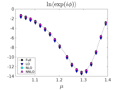
Figure 9: Comparison of the phase factor expectation value, computed with the “full theory”, with the result from the Advanced Moments method. We observe that the moment expansion rapidly converges with the NNLO and NNLO lie on top of each other and are indistinguishable from the full answer. Statistical error bars are included.

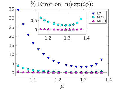
Figure 10: Relative difference between the moment approximation and the full answer. As expected, the approximation works better in the strong sign problem regime

$\mu$	$\ln\langle\exp(i\phi)\rangle$	LO ($\%$)	NLO ($\%$)	NNLO ($\%$)
1.042	-1.271(2)	36	4.1	0.48
1.062	-1.588(3)	27	2.6	0.22
1.082	-1.993(3)	21	1.8	0.11
1.102	-2.52(0)	16	1.3	0.07
1.122	-3.213(5)	13	1.0	0.05
1.142	-4.019(10)	10	0.8	0.04
1.162	-5.02(1)	8	0.7	0.03
1.182	-6.251(10)	7	0.5	0.02
1.202	-7.602(25)	5	0.4	0.02
1.232	-9.823(66)	4	0.3	0.02
1.252	-11.43(5)	4	0.3	0.01
1.272	-12.56(6)	3	0.3	0.01
1.292	-13.0(2)	3	0.3	0.01
1.312	-12.76(7)	3	0.3	0.01
1.332	-11.29(4)	4	0.3	0.01
1.352	-8.811(13)	5	0.4	0.02
1.372	-5.639(20)	7	0.6	0.03
1.392	-2.756(8)	15	1.2	0.06

Table 5: Logarithm of the phase factor expectation value from  Garron:2016noc and relative precision obtained with the moment method for the various orders as a function of $\mu$.

6 Conclusions

There are two main possibilities in addressing finite density quantum field theory: (i) facing the large cancellations that give rise to the smallness of the partition function or (ii) to reformulate to an equivalent theory say by dualisation Gattringer:2014nxa or by a complexfication of the fields Aarts:2013lcm . Method (ii) would be preferred if the approach exists and if exactness can be guaranteed. The appeal of method (i) is that it is universally applicable if a way is found to control the cancellations.

A first success for direction (i) emerged with the advent of Wang-Landau type techniques and, most notably, the LLR method Langfeld:2012ah : due to the feature of exponential error suppression of the LLR approach Langfeld:2015fua , high precision data for the density-of-states $\rho(s)$ of finding a particular phase $s$ over many orders of magnitude has become available. The partition function now emerges as Fourier transform of $\rho(s)$. Due to large cancellations, this Fourier transform is a challenge in its own right. The recent success reported in Langfeld:2014nta and in Garron:2016noc hinge on the ability to find a fit function for $\ln\rho(s)$ that well represents hundreds of numerical data points with relatively few fit parameters. This situation is unsatisfactory since the quest for this fit function might not be always successful.

The present paper explores three methods to perform the Fourier transform:

• The Gaussian approximation of the extensive density-of-states $\rho_{E}$ is most easily implemented, but hard to improve in a systematic way. For the example of HDQCD, we found this approximation yields the right order of magnitude through out and only misses the exact phase factor by a factor of two when the sign problem is strongest.

• The telegraphic approximation yields the phase factor through an alternating (discrete) sum of the extensive density-of-states $\rho_{E}$. The relative systematic error is of the order of the phase factor itself, which makes the approximation excellent in the strong sign-problem regime.

• The advanced moment approach is a systematic expansion of this Fourier transform with respect to the deviations of $\rho(s)$ from uniformity. The expansion therefore works best in the strong-sign problem regime. The expansion is independent of the quantum field theory setting an can be applied to the Fourier transform of any sufficiently smooth function $\rho(s)$, $s\in[-\pi,\pi]$. At the heart of expansion are the so-called Advanced Moments. We have thoroughly derived these moments and the theory independent expansion coefficients $\alpha$. We found evidence that the expansion coefficients decrease exponentially with increasing order, thus guaranteeing rapid convergence if $\rho(s)$ admits moments $M$ that are bounded. We have tested and validated the Advanced Moment expansion in the context of HDQCD: we have confirmed that the expansion converges very quickly. It works best in the strong-sign problem region as expected, although at third order the results agree with the “full” answer at the sub-percent level even in the weak sign problem regime.

Acknowledgements: We are grateful to B. Lucini and A. Rago for helpful discussions. NG and KL are supported by the Leverhulme Trust (grant RPG-2014-118) and, KL by STFC (grant ST/L000350/1).

References

• (1) K. Fukushima, T. Hatsuda, The phase diagram of dense QCD, Rept. Prog. Phys. 74 (2011) 014001. arXiv:1005.4814, doi:10.1088/0034-4885/74/1/014001.
• (2) P. de Forcrand, Simulating QCD at finite density, PoS LAT2009 (2009) 010. arXiv:1005.0539.
• (3) S. Gupta, QCD at finite density, PoS LATTICE2010 (2010) 007. arXiv:1101.0109.
• (4) L. Levkova, QCD at nonzero temperature and density, PoS LATTICE2011 (2011) 011. arXiv:1201.1516.
• (5) G. Aarts, Complex Langevin dynamics and other approaches at finite chemical potential, PoS LATTICE2012 (2012) 017. arXiv:1302.3028.
• (6) C. Gattringer, New developments for dual methods in lattice field theory at non-zero density, PoS LATTICE2013 (2014) 002. arXiv:1401.7788.
• (7) D. Sexty, New algorithms for finite density QCD, PoS LATTICE2014 (2014) 016. arXiv:1410.8813.
• (8) S. Borsányi, Fluctuations at finite temperature and density, PoS LATTICE2015 (2016) 015. arXiv:1511.06541.
• (9) K. Langfeld, Density-of-states, in: Proceedings, 34th International Symposium on Lattice Field Theory (Lattice 2016): Southampton, UK, July 24-30, 2016, 2016. arXiv:1610.09856.
• (10) M. Troyer, U.-J. Wiese, Computational complexity and fundamental limitations to fermionic quantum Monte Carlo simulations, Phys. Rev. Lett. 94 (2005) 170201. arXiv:cond-mat/0408370, doi:10.1103/PhysRevLett.94.170201.
• (11) K. Langfeld, B. Lucini, A. Rago, The density of states in gauge theories, Phys. Rev. Lett. 109 (2012) 111601. arXiv:1204.3243, doi:10.1103/PhysRevLett.109.111601.
• (12) K. Langfeld, B. Lucini, R. Pellegrini, A. Rago, An efficient algorithm for numerical computations of continuous densities of states, Eur. Phys. J. C76 (6) (2016) 306. arXiv:1509.08391, doi:10.1140/epjc/s10052-016-4142-5.
• (13) K. Langfeld, J. M. Pawlowski, Two-color QCD with heavy quarks at finite densities, Phys. Rev. D88 (7) (2013) 071502. arXiv:1307.0455, doi:10.1103/PhysRevD.88.071502.
• (14) B. Lucini, W. Fall, K. Langfeld, Overcoming strong metastabilities with the LLR method, in: Proceedings, 34th International Symposium on Lattice Field Theory (Lattice 2016): Southampton, UK, July 24-30, 2016, 2016. arXiv:1611.00019.
• (15) K. Langfeld, B. Lucini, Density of states approach to dense quantum systems, Phys. Rev. D90 (9) (2014) 094502. arXiv:1404.7187, doi:10.1103/PhysRevD.90.094502.
• (16) N. Garron, K. Langfeld, Anatomy of the sign-problem in heavy-dense QCD, Eur. Phys. J. C76 (10) (2016) 569. arXiv:1605.02709, doi:10.1140/epjc/s10052-016-4412-2.
• (17) S. Ejiri, On the existence of the critical point in finite density lattice QCD, Phys. Rev. D77 (2008) 014508. arXiv:0706.3549, doi:10.1103/PhysRevD.77.014508.
• (18) Y. Nakagawa, S. Ejiri, S. Aoki, K. Kanaya, H. Ohno, H. Saito, T. Hatsuda, T. Umeda, Histogram method in finite density QCD with phase quenched simulations, PoS LATTICE2011 (2011) 208. arXiv:1111.2116.
• (19) H. Saito, S. Aoki, K. Kanaya, H. Ohno, S. Ejiri, Y. Nakagawa, T. Hatsuda, T. Umeda, Finite density QCD phase transition in the heavy quark region, PoS LATTICE2011 (2011) 214. arXiv:1202.6113.
• (20) H. Saito, S. Ejiri, S. Aoki, K. Kanaya, Y. Nakagawa, H. Ohno, K. Okuno, T. Umeda, Histograms in heavy-quark QCD at finite temperature and density, Phys. Rev. D89 (3) (2014) 034507. arXiv:1309.2445, doi:10.1103/PhysRevD.89.034507.
• (21) J. Greensite, J. C. Myers, K. Splittorff, The density in the density of states method, JHEP 10 (2013) 192. arXiv:1308.6712, doi:10.1007/JHEP10(2013)192.
• (22) S. Ejiri, S. Aoki, T. Hatsuda, K. Kanaya, Y. Nakagawa, H. Ohno, H. Saito, T. Umeda, Numerical study of QCD phase diagram at high temperature and density by a histogram method, Central Eur. J. Phys. 10 (2012) 1322–1325. arXiv:1203.3793, doi:10.2478/s11534-012-0054-7.
• (23) S. Ejiri, Y. Nakagawa, S. Aoki, K. Kanaya, H. Saito, T. Hatsuda, H. Ohno, T. Umeda, Probability distribution functions in the finite density lattice QCD, PoS LATTICE2012 (2012) 089. arXiv:1212.0762.
• (24) S. Ejiri, Phase structure of hot dense QCD by a histogram method, Eur. Phys. J. A49 (2013) 86. arXiv:1306.0295, doi:10.1140/epja/i2013-13086-7.
• (25) N. Garron, K. Langfeld, Tackling the sign problem with a moment expansion and application to Heavy dense QCD, in: Proceedings, 34th International Symposium on Lattice Field Theory (Lattice 2016): Southampton, UK, July 24-30, 2016, 2016. arXiv:1611.01378.